Multigoal-Oriented Error Estimates for Non-linear Problems

Abstract

In this work, we further develop multigoal-oriented a posteriori error estimation with two objectives in mind. First, we formulate goal-oriented mesh adaptivity for multiple functionals of interest for nonlinear problems in which both the Partial Differential Equation (PDE) and the goal functionals may be nonlinear. Our method is based on a posteriori error estimates in which the adjoint problem is used and a partition-of-unity is employed for the error localization that allows us to formulate the error estimator in the weak form. We provide a careful derivation of the primal and adjoint parts of the error estimator. The second objective is concerned with balancing the nonlinear iteration error with the discretization error yielding adaptive stopping rules for Newton’s method. Our techniques are substantiated with several numerical examples including scalar PDEs and PDE systems, geometric singularities, and both nonlinear PDEs and nonlinear goal functionals. In these tests, up to six goal functionals are simultaneously controlled.

1 Introduction

A posteriori error estimation and mesh adaptivity are well-developed methodologies for finite element computations, see, e.g., the monographs [49, 2, 7, 38, 25, 42] and the references therein. Specifically, goal-oriented error estimation is a powerful method when the evaluation of certain functionals of interest (often these are technical quantities) is the main aim rather than the computation of global error norms. Here, the dual-weighted residual (DWR) method is often applied [9, 10].

Thanks to increasing computational resources, multiphysics applications such as multiphase flow, porous media applications, fluid-structure interaction and electromagnectics are currently one main focus in applied mathematics and engineering. Here, mesh adaptivity (ideally combined with parallel computing) can greatly reduce the computational cost while measuring functionals of interest with sufficient accuracy. Since in multiphysics, several physical phenomena interact, it might be desirable that more than one goal functional shall be controlled. However, only a few studies have appeared yet. A first methodology was proposed in [27, 26]. Other studies can be found in [29, 39] and more recently in [48, 20, 31].

Until a few years ago, one principle problem in using the DWR method was the fact that the error estimator was based on the strong form of the equations [10] or the weak form using special interpolation operators working on patched meshes [12]. In [44], the previous localization techniques were analyzed in more detail and additionally a novel localization strategy based on a partition-of-unity (PU) was proposed. The PU localization specifically allows for a much simpler application of the DWR method to multiphysics and nonlinear, vector-valued equations [44, 51]. In addition, the PU-DWR method works well with other discretization techniques such as BEM-based FEM [50] or the finite cell method [46]. On the other hand, the methodology of the PU-DWR method with multiple goal functionals has recently been worked out for linear, scalar-valued problems in [20].

The first goal of this paper is to extend this work to nonlinear problems and PDE systems. Here, our focus is on a careful design of the error estimator that includes both the primal part and the adjoint part. The latter one is often neglected in the literature because the evaluation requires additional computational cost and renders the method even more expensive. It is clear and well-known (see e.g., [10]) that, in the linear case, the primal and adjoint residuals yield the same error values, but possibly different locally refined meshes; see e.g. [44]. In our current work, we will see that the adjoint estimator part is crucial to obtain good effectivity indices. Therefore, this term should not be neglected.

The second objective of this paper is concerned with balancing the discretization and the nonlinear iteration error. In recent years, there has been published some work on balancing the iteration error (of the linear or nonlinear solver) with the discretization error [21, 8, 37, 40, 41]. We base ourselves on [40], and we employ specifically the PU localization. Consequently, the DWR method is used to design an adaptive stopping criterion for Newton’s method that is in balance with the estimated discretization error. The main aspects comprise a careful choice of the weighting functions to design an appropriate joined goal functional. Moreover, we provide all details for the nonlinear solver, which is a Newton-type method with backtracking line-search. Since we know a solution on the previous mesh, we use this solution as initial guess for Newton’s method yielding a nested iteration. Specifically, nested solution methods or nonlinear nested iterations were developed, for instance, in [10, 24]. We refer to [24, 43] for the analysis of nested iteration methods.

In summary, the goals of this work are two-fold:

• Design of the PU-DWR method for multigoal-oriented error estimation for nonlinear problems and PDE systems.

• Balancing iteration and discretization errors for nonlinear multigoal-oriented error estimation and mesh adaptivity. The nonlinearities may appear in the PDE itself as well as in the goal functionals.

The outline of this is paper is as follows: In Section 2, our setting is described. Next, in Section 3, we describe the methodology for one goal functional. This is followed by a detailed derivation of a multigoal-oriented approach presented in Section 4. The key algorithms are formulated in Section 5. In Section 6 several numerical tests substantiate our developments. We summarize our work in Section 7.

2 An abstract setting

Let $U$ and $V$ be Banach spaces, and let $\mathcal{A}:U\mapsto V^{*}$ be a (possibly) nonlinear operator, where $V^{*}$ denotes the dual space of the Banach space $V$. We have in mind nonlinear differential operators $\mathcal{A}$ acting between Sobolev spaces. We now consider the following weak formulation of the operator equation $\mathcal{A}(u)=0$ in $V^{*}$: Find $u\in U$ such that

$$\mathcal{A}(u)(v)=0\quad\forall v\in V.$$ (1)

The discretization of the nonlinear variational problem (1) can be performed by means of different methods. Our favored method is the Finite Element Method (FEM), see also Section 5.1. The corresponding discrete problem reads as follows: Find $u_{h}\in U_{h}$ such that

$$\mathcal{A}(u_{h})(v_{h})=0\quad\forall v_{h}\in V_{h},$$ (2)

where $U_{h}$ and $V_{h}$ are finite-dimensional subspaces of $U$ and $V$, respectively. For the time being, let us assume that both problems are solvable. Later we will specify our assumptions imposed on $\mathcal{A}$. We are primarily not interested in approximating a solution $u$ of (1), but in the approximate computation of one or more possibly nonlinear functionals at a solution.

An example for such an operator $\mathcal{A}$ is given by the weak formulation of the regularized $p$-Laplace equation (see also [19, 28, 47]) that reads as follows: Find $u\in U:=W^{1,p}_{0}(\Omega)$ such that

$$\mathcal{A}(u)(v):= \langle{(\varepsilon^{2}+|\nabla u|^{2})^{\frac{p-2}{2}}\nabla u,\nabla v\rangle}_{(L^{p}(\Omega))^{*}\times L^{p}(\Omega)}-\langle{f,v\rangle}_{(W^{1,p}_{0}(\Omega))^{*}\times W^{1,p}_{0}(\Omega)}=0$$ (3)

for all $v\in V:=W^{1,p}_{0}(\Omega)$, where $\varepsilon$ denotes a fixed positive regularization parameter, $f\in(W^{1,p}_{0}(\Omega))^{*}=W^{-1,q}(\Omega)$ is some given source, with $p^{-1}+q^{-1}=1$ and fixed $p>1$, and $\langle{\cdot,\cdot}\rangle$ denots the corresponding duality products. Here, $\Omega\subset\mathbb{R}^{d}$, $d=1,2,3$, is a bounded Lipschitz domain, and $W^{1,p}_{0}(\Omega)$ denotes the usual Sobolev space of all functions from the Lebesgue space $L^{p}(\Omega)$ with weak derivatives in $L^{p}(\Omega)$ and trace zero on the boundary $\partial\Omega$, see, e.g., [1]. The notation $|\cdot|$ is used for the Euclidean norm of some vector. The corresponding strong form is formally given by

$$-\text{div}((\varepsilon^{2}+|\nabla u|^{2})^{\frac{p-2}{2}}\nabla u) =f\quad\mbox{in}\;\Omega,$$

$$u =0\quad\mbox{on}\;\partial\Omega.$$

In Subsection 6.2, the regularized $p$-Laplace (3) serves as first example for our numerical experiments.

Remark 2.1.

We refer the reader to [23] for the investigation of the original $p$-Laplace problem.

3 The dual weighted residual method for nonlinear problems in the case of a single-goal functional

In this section, we apply the DWR method to nonlinear problems. The general method was developed in [10]. The extension to balance discretization and iteration errors was undertaken in [37, 41, 40]. We base ourselves on the latter study [40], in which algorithms for nonlinear problems have been worked out. This last paper, together with [44, 20], form the basis of the current paper. We are interested in the goal functional evaluation $J:U\to\mathbb{R}$ with $u\mapsto J(u)$, where $u\in U$ is a solution of the primal problem (1). Examples for such goal functionals are:

• point evaluation:

  $$J(u):=u(x_{0}),$$

• integral evaluation:

  $$J(u):=\int_{\Omega}u(x)\xi(x)\,dx,$$

• nonlinear functional evaluation:

  $$J(u):=\int_{\Omega}u(x)\xi(x)u(x_{0})^{2}\,dx\int_{\Omega}u(y)\phi(y)\,dy,$$

where $\xi$ and $\phi$ are given functions from $L^{2}(\Omega)$ and $x_{0}$ a given point in $\Omega$. For the DWR approach we need to solve the adjoint problem: Find $z\in V$ corresponding to $u\in U$ such that

$$\mathcal{A}^{\prime}(u)(v,z)=J^{\prime}(u)(v)\quad\forall v\in U,$$ (4)

where $u$ denotes a (primal) solution of the primal problem (1), and $\mathcal{A^{\prime}}(u)$ and $J^{\prime}(u)$ denote the Fréchet-derivatives of the nonlinear operator or functional, respectively, evaluated at $u$. Later we also need the corresponding discrete solution of the adjoint problem. This reads as follows: Find $z_{h}\in V_{h}$ corresponding to $u_{h}\in U_{h}$ such that

$$\mathcal{A}^{\prime}(u_{h})(v_{h},z_{h})=J^{\prime}(u_{h})(v_{h})\quad\forall v_{h}\in U_{h},$$ (5)

with $u_{h}$ as a solution of (2).

Similarly to the findings in [40, 10, 41] for the Galerkin case ($U=V$), we derive an error representation in the following theorem:

Theorem 3.1.

Let us assume that $\mathcal{A}\in\mathcal{C}^{3}(U,V)$ and $J\in\mathcal{C}^{3}(U,\mathbb{R})$. If $u$ solves (1) and $z$ solves (4) for $u\in U$, then it holds for arbitrary fixed $\tilde{u}\in U$ and $\tilde{z}\in V$ :

$$\begin{split}J(u)-J(\tilde{u})&=\frac{1}{2}\rho(\tilde{u})(z-\tilde{z})+\frac{1}{2}\rho^{*}(\tilde{u},\tilde{z})(u-\tilde{u})-\rho(\tilde{u})(\tilde{z})+\mathcal{R}^{(3)},\end{split}$$ (6)

where

$$\rho(\tilde{u})(\cdot) :=-\mathcal{A}(\tilde{u})(\cdot),$$ (7)

$$\rho^{*}(\tilde{u},\tilde{z})(\cdot) :=J^{\prime}(u)-\mathcal{A}^{\prime}(\tilde{u})(\cdot,\tilde{z}),$$ (8)

and the remainder term

$$\begin{split}\mathcal{R}^{(3)}:=\frac{1}{2}\int_{0}^{1}[J^{\prime\prime\prime}(\tilde{u}+se)(e,e,e)-\mathcal{A}^{\prime\prime\prime}(\tilde{u}+se)(e,e,e,\tilde{z}+se^{*})-3\mathcal{A}^{\prime\prime}(\tilde{u}+se)(e,e,e)]s(s-1)\,ds,\end{split}$$ (9)

with $e=u-\tilde{u}$ and $e^{*}=z-\tilde{z}$.

Proof.

For the completeness of the presentation we add the proof below, which is very similar to [40]. First we define $x:=(u,z)\in X:=U\times V$ and $\tilde{x}:=(\tilde{u},\tilde{v})\in X$. By assuming that $\mathcal{A}\in\mathcal{C}^{3}(U,V)$ and $J\in\mathcal{C}^{3}(U,\mathbb{R})$ we know that the Lagrange function

$$\mathcal{L}(\hat{x}):=J(\hat{u})-\mathcal{A}(\hat{u})(\hat{z})\quad\forall(\hat{u},\hat{z})=:\hat{x}\in X,$$

is in $\mathcal{C}^{3}(X,\mathbb{R})$. Assuming this it holds

$$\mathcal{L}(x)-\mathcal{L}(\tilde{x})=\int_{0}^{1}\mathcal{L}^{\prime}(\tilde{x}+s(x-\tilde{x}))(x-\tilde{x})\,ds.$$

Using the trapezoidal rule [40], we obtain

$$\int_{0}^{1}f(s)\,ds=\frac{1}{2}(f(0)+f(1))+\frac{1}{2}\int_{0}^{1}f^{\prime\prime}(s)s(s-1)\,ds,$$

for $f(s):=\mathcal{L}^{\prime}(\tilde{x}+s(x-\tilde{x}))(x-\tilde{x})$ we conclude

$$\mathcal{L}(x)-\mathcal{L}(\tilde{x})= \frac{1}{2}(\mathcal{L}^{\prime}(x)(x-\tilde{x})+\mathcal{L}^{\prime}(\tilde{x})(x-\tilde{x}))+\mathcal{R}^{(3)}.$$

From the definition of $\mathcal{L}$ we observe that

$$J(u)-J(\tilde{u})=\mathcal{L}(x)-\mathcal{L}(\tilde{x})+\underbrace{A(u)(z)}_{=0}+A(\tilde{u})(\tilde{z})= \frac{1}{2}(\mathcal{L}^{\prime}(x)(x-\tilde{x})+\mathcal{L}^{\prime}(\tilde{x})(x-\tilde{x}))+A(\tilde{u})(\tilde{z})+\mathcal{R}^{(3)}.$$

It remains to show that $\frac{1}{2}(\mathcal{L}^{\prime}(x)(x-\tilde{x})+\mathcal{L}^{\prime}(\tilde{x})(x-\tilde{x}))=\frac{1}{2}\rho(\tilde{u})(z-\tilde{z})+\frac{1}{2}\rho^{*}(\tilde{u},\tilde{z})(u-\tilde{u})$. But this is true since

$$\mathcal{L}^{\prime}(x)(x-\tilde{x})+\mathcal{L}^{\prime}(\tilde{x})(x-\tilde{x})= \underbrace{J^{\prime}(u)(e)-\mathcal{A}^{\prime}(u)(e,z)}_{=0}-\underbrace{A(u)(e^{*})}_{=0}+\underbrace{J^{\prime}(\tilde{u})(e)-\mathcal{A}^{\prime}(\tilde{u})(e,\tilde{z})}_{=\rho^{*}(\tilde{u},\tilde{z})(u-\tilde{u})}-\underbrace{A(\tilde{u})(e^{*})}_{=-\rho(\tilde{u})(z-\tilde{z})}.$$

∎

Remark 3.2.

Instead of $\mathcal{A}\in\mathcal{C}^{3}(U,V)$ and $J\in\mathcal{C}^{3}(U,\mathbb{R})$ it is sufficient that $\mathcal{A}\in\mathcal{C}^{2}(U,V)$, $J\in\mathcal{C}^{2}(U,\mathbb{R})$ and $J^{\prime\prime\prime},$ $\mathcal{A^{\prime\prime\prime}}$ exist and are bounded. Moreover one can further relax these assumptions. Indeed the boundedness of the derivatives is just needed in the set $\{w\in U|w=(1-s)u+s\tilde{u}\}$ and just in direction $u-\tilde{u}$.

Remark 3.3.

It might happen that $\mathcal{A}\in\mathcal{C}^{3}(U,V)$ and $J\in\mathcal{C}^{3}(U,\mathbb{R})$ do not hold for the continuous spaces. Since the result holds for general Banach spaces $U$ and $V$, it is sufficient to be shown for the discrete spaces $U_{h,u},V_{h,z}$, where $U_{h,u}:=\{w+cu|w\in U_{h},c\in\mathbb{R}\},V_{h,z}:=\{v+cz|v\in V_{h},c\in\mathbb{R}\}$.

Remark 3.4.

In accordance with the literature, we denote the parts $\rho(\tilde{u})(z-\tilde{z})$ and $\rho^{*}(\tilde{u},\tilde{z})(u-\tilde{u})$ by primal error estimator and adjoint error estimator, respectively. The remainder term $\mathcal{R}^{(3)}$, as in (9), is of the order $\mathcal{O}(\|e\|_{U}^{2}\text{max}(\|e\|_{U},\|e^{*}\|_{V}))$. Therefore, it can be neglected if $\{\tilde{u},\tilde{z}\}$ are close enough to $\{u,z\}$.

As in [40] ,we can identify

$$\eta_{h}:=|\frac{1}{2}\rho(\tilde{u})(z-\tilde{z})+\frac{1}{2}\rho^{*}(\tilde{u},\tilde{z})(u-\tilde{u})|,$$ (10)

as the discretization error and

$$\eta_{m}:=|\rho(\tilde{u})(\tilde{z})|,$$ (11)

as the linearization error if we neglect the remainder term $\mathcal{R}^{(3)}$. Since Theorem 3.1 is valid for arbitrary $\tilde{z}$ and $\tilde{u}$ it also holds for approximations $u_{h}$ and $z_{h}$, even if they are not computed exactly. Of course, formula (10) still contains an exact solution $u$. Since $u$ is not known, we either use an approximation in an enriched discrete space (for example, in a finite element space, with higher polynomial degree), or we use an interpolant $I_{h}^{h_{2}}$, such as in [10], to obtain a more accurate solution $u_{h}^{(2)}$. If not mentioned otherwise, we use the approximation in the enriched (finite element) space. An enriched discrete space is also used to compute an approximation $z_{h}^{(2)}$ of $z$. If one would use the same finite-dimensional space as for the test space used in the discrete primal problem (2), then $\mathcal{A}(u_{h})(z_{h})=0$ for our approximate solution $u_{h}$ of (2) (if the nonlinear problem is solved exactly). Therefore, the discrete adjoint problem reads as follows: Find $z_{h}^{(2)}\in V_{h}^{(2)}$ such that

$$\mathcal{A}^{\prime}(u_{h}^{(2)})(v_{h}^{(2)},z_{h}^{(2)})=J^{\prime}(u_{h}^{(2)})(v_{h}^{(2)})\quad\forall v_{h}^{(2)}\in U_{h}^{(2)},$$ (12)

where $U_{h}^{(2)}$ and $V_{h}^{(2)}$ denote the enriched finite dimensional spaces, and $u_{h}^{(2)}$ denotes the more accurate solution, obtained by solving (2) with $U_{h}=U_{h}^{(2)}$ and $V_{h}=V_{h}^{(2)}$ or by interpolation $u_{h}^{(2)}=I_{h}^{h_{2}}u_{h}$. With these approximations, the practical error estimator reads:

$$\eta_{h}:=|\frac{1}{2}\rho(u_{h})(z_{h}^{(2)}-z_{h})+\frac{1}{2}\rho^{*}(u_{h},z_{h})(u_{h}^{(2)}-u_{h})|.$$ (13)

For localization of the error estimator, we use the partition of unity (PU) technique which is presented in [44]. This means that we choose a set of functions $\{\psi_{1},\psi_{2},\cdots,\psi_{N}\}$ such that $\sum_{i=1}^{N}\psi_{i}\equiv 1.$ Inserting this into (13) leads to

$$\eta_{h}:=|\sum_{i=1}^{N}\eta_{i}|,$$ (14)

with

$$\eta_{i}:=\frac{1}{2}\rho(\tilde{u})((z_{h}^{(2)}-\tilde{z})\psi_{i})+\frac{1}{2}\rho^{*}(\tilde{u},\tilde{z})((u_{h}^{(2)}-\tilde{u})\psi_{i}).$$ (15)

We notice that in the primal part of the error indicator $\tilde{z}$ is replaced by $i_{h}z_{h}^{(2)}$ as in [10]. For instance, a typical partition of unity is given by the finite element basis. In this case, we distribute $|\eta_{i}|$ to the corresponding elements with a certain weight as for example illustrated in Figure 1.

Figure 1: Equal distribution of the local error estimator using the $Q^{1}_{c}$ basis function at the central vertex to the corresponding elements as in [44], see also Section 5.1.

4 Multiple-goal functionals

Now let us assume that we are interested in the evaluation of $N$ functionals, which we denote by $J_{1},J_{2},\ldots,J_{N}$. From Section 3, we know how to compute a local error estimator for one functional. We could compute the local error estimators separately. However, we would have to solve the adjoint problem (4) $N$ times [27, 26]. Let us now assume that a solution $u$ of problem (1) and the chosen $\tilde{u}\in U$ belong to $\bigcap_{i=1}^{N}\mathcal{D}(J_{i})$, where $\mathcal{D}(J_{i})$ describes the domain of $J_{i}$.

Definition 4.1 (error-weighting function).

Let $M\subseteq\mathbb{R}^{N}$. We say that $\mathfrak{E}:(\mathbb{R}^{+}_{0})^{N}\times M\mapsto\mathbb{R}^{+}_{0}$ is an error-weighting function if $\mathfrak{E}(\cdot,m)\in\mathcal{C}^{1}((\mathbb{R}^{+}_{0})^{N},\mathbb{R}^{+}_{0})$ is strictly monotonically increasing in each component and $\mathfrak{E}(0,m)=0$ for all $m\in M$.

Let $\vec{J}:\bigcap_{i=1}^{N}\mathcal{D}(J_{i})\subseteq U\mapsto\mathbb{R}^{N}$ be defined as $\vec{J}(v):=(J_{1}(v),J_{2}(v),\cdots,J_{N}(v))$ for all $v\in\bigcap_{i=1}^{N}\mathcal{D}(J_{i})$. Furthermore, we define the operation $|\cdot|_{N}:\mathbb{R}^{N}\mapsto(\mathbb{R}^{+}_{0})^{N}$ as $|x|_{N}:=(|x_{1}|,|x_{2}|,\cdots,|x_{N}|)$ for $x\in\mathbb{R}^{N}$. This allows us to define the error functional as follows

$$\tilde{J}_{\mathfrak{E}}(v):=\mathfrak{E}(|\vec{J}(u)-\vec{J}(v)|_{N},\vec{J}(\tilde{u}))\qquad\forall v\in\bigcap_{i=1}^{N}\mathcal{D}(J_{i}).$$ (16)

It is trivial to see from the definition of $\mathfrak{E}$ that $J_{\mathfrak{E}}(v)\in\mathbb{R}^{+}_{0}$ for all $v\in\bigcap_{i=1}^{N}\mathcal{D}(J_{i})$.

Remark 4.2.

The idea of the construction of $\tilde{J}_{\mathfrak{E}}(v)$ is that $\mathfrak{E}(|\vec{J}(u)-\vec{J}(v)|_{N},\vec{J}(\tilde{u}))$ is a semi-metric (as in [45, 32]) on the set of equivalence classes $(\vec{J})^{-1}(\mathcal{R}(\vec{J})):=\{(\vec{J})^{-1}(x):x\in\mathcal{R}(\vec{J})\}$, where $(\vec{J})^{-1}(x):=\{v\in\bigcap_{i=1}^{N}\mathcal{D}(J_{i}):\vec{J}(v)=x\}$, with $\mathcal{R}(\vec{J})$ denotes the range of $\vec{J}$, measuring the distance between the equivalence classes containing $u$ and $v$. Hence, $\tilde{J}_{\mathfrak{E}}(v)$ represents a semi-metric distance which ensures that $\tilde{J}_{\mathfrak{E}}$ is monotonically increasing if $|J_{i}(u)-J_{i}(\tilde{u})|$ is monotonically increasing.

Remark 4.3.

If we drop the monotonicity condition in the definition of $\mathfrak{E}$, then, for example,

$$\mathfrak{E}(|\vec{J}(u)-\vec{J}(v)|_{N},\vec{J}(\tilde{u})):=\prod_{i=0}^{N}|J_{i}(u)-J_{i}(v)|,$$

would be an error-weighting function, resulting in $J_{\mathfrak{E}}(\tilde{u})=0$ iff $J_{i}(u)=J_{i}(\tilde{u})$ at least for one $i\in\{1,2,\cdots,N\}$.

Remark 4.4.

The derivation given in this section holds for a general $\tilde{u}$ such that $\vec{J}(\tilde{u})\in M$. In particular, we are interested in $\tilde{u}$ to be an approximation to $u_{h}$ solving (2).

The weak derivative of (16) in $U$ at $\tilde{u}$ is given by

$$\tilde{J}_{\mathfrak{E}}^{\prime}(\tilde{u})(v):=-\sum_{i=1}^{N}\text{ sign}(J_{i}(u)-J_{i}(\tilde{u}))\frac{\partial\mathfrak{E}}{\partial x_{i}}(|\vec{J}(u)-\vec{J}(\tilde{u})|_{N},\vec{J}(\tilde{u}))J_{i}^{\prime}(\tilde{u})(v)\qquad\forall v\in\mathcal{D}(\tilde{J}_{\mathfrak{E}}^{\prime}(\tilde{u})),$$ (17)

with

$$\text{sign}(x):=\begin{cases}\frac{x}{|x|},\quad\text{for }x\not=0,\\ 0\quad else\end{cases}$$ (18)

In [27, 26, 20], the functionals where combined as follows

$$\tilde{J}_{c}(v):=\sum_{i=1}^{N}\underbrace{\frac{\omega_{i}\text{ sign}(J_{i}(u)-J_{i}(\tilde{u}))}{|J_{i}(\tilde{u})|}}_{=:w_{i}}J_{i}(v)\quad\forall v\in\bigcap_{i=0}^{N}\mathcal{D}(J_{i}).$$ (19)

Carefully inspecting [26], we see that the following result can be established:

Proposition 4.1.

If $\tilde{J}_{c}$ is defined as in (19) and $\tilde{J}_{\mathfrak{E}}$ as in (16), then we have

$$\tilde{J}_{c}(u)-\tilde{J}_{c}(\tilde{u}) =\tilde{J}_{\mathfrak{E}}(\tilde{u}),$$ (20)

$$-\tilde{J}_{c}^{\prime}(\tilde{u})(v) =\tilde{J}_{\mathfrak{E}}^{\prime}(\tilde{u})(v),\qquad\forall v\in\mathcal{D}(\tilde{J}_{c}^{\prime}(\tilde{u}))\cap\mathcal{D}(\tilde{J}_{\mathfrak{E}}^{\prime}(\tilde{u})),$$ (21)

$$\mathcal{D}(\tilde{J}_{c}^{\prime}(\tilde{u})) =\mathcal{D}(\tilde{J}_{\mathfrak{E}}^{\prime}(\tilde{u}))$$ (22)

with $\mathfrak{E}(x,\vec{J}(\tilde{u})):=\sum_{i=1}^{N}\frac{\omega_{i}x_{i}}{|J_{i}(\tilde{u})|}$.

Proof.

First we conclude that

$$\tilde{J}_{c}(u)-\tilde{J}_{c}(\tilde{u}) =\sum_{i=1}^{N}\frac{\omega_{i}\text{ sign}(J_{i}(u)-J_{i}(\tilde{u}))}{|J_{i}(\tilde{u})|}(J_{i}(u)-J_{i}(\tilde{u}))$$

$$=\sum_{i=1}^{N}\frac{\omega_{i}|J_{i}(u)-J_{i}(\tilde{u})|}{|J_{i}(\tilde{u})|}$$

$$=\mathfrak{E}(|\vec{J}(u)-\vec{J}(\tilde{u})|_{N},\vec{J}(\tilde{u}))=\tilde{J}_{\mathfrak{E}}(\tilde{u}),$$

which already shows (20). The weak derivative of $\tilde{J}_{c}$ is given by

$$\tilde{J}_{c}^{\prime}(\tilde{u})(v)=\sum_{i=1}^{N}\frac{\omega_{i}\text{ sign}(J_{i}(u)-J_{i}(\tilde{u}))}{|J_{i}(\tilde{u})|}J_{i}^{\prime}(\tilde{u})(v).$$ (23)

From $\frac{\partial\mathfrak{E}}{\partial x_{i}}(|\vec{J}(u)-\vec{J}(\tilde{u})|_{N},\vec{J}(\tilde{u}))=\frac{\omega_{i}}{|J_{i}(\tilde{u})|}$ for all $i\in\{1,2,\cdots,N\}$, and because (23) and (17) coincide up to the sign, it holds that (21) and (22) are valid. ∎

Remark 4.5.

$\mathfrak{E}(x,\vec{J}(\tilde{u})):=\sum_{i=1}^{N}\frac{\omega_{i}x_{i}}{|J_{i}(\tilde{u})|}$ is an error-weighting function with $M:=\{x\in\mathbb{R}^{N}:\min(|x|)>0\}$ provided that $\omega_{i}>0$ for all $i=1,2,\ldots,N$.

Remark 4.6.

Proposition 4.1 does not use the property that $u$ solves (1). We just need that $u\in\bigcap_{i=0}^{N}\mathcal{D}(J_{i})$. However, the goal is to measure the error to an exact solution.

Since an exact solution $u$ is not known, neither $\tilde{J}_{c}$ nor $\tilde{J}_{\mathfrak{E}}$ can be constructed. As in Section 3, we use the approximation $u_{h}^{(2)}$ instead of an exact solution $u$ to approximate $\tilde{J}_{c}$ or $\tilde{J}_{\mathfrak{E}}$ by $J_{c}$ and $J_{\mathfrak{E}}$, respectively. This approximation reads as follows

$$J_{\mathfrak{E}}(v):=\mathfrak{E}(|\vec{J}(u_{h}^{(2)})-\vec{J}(v)|_{N},\vec{J}(\tilde{u}))\qquad\forall v\in\bigcap_{i=1}^{N}\mathcal{D}(J_{i}),$$ (24)

with the derivative

$$J_{\mathfrak{E}}^{\prime}(\tilde{u})(v):=-\sum_{i=1}^{N}\text{ sign}(J_{i}(u_{h}^{(2)})-J_{i}(\tilde{u}))\frac{\partial\mathfrak{E}}{\partial x_{i}}(|\vec{J}(u_{h}^{(2)})-\vec{J}(\tilde{u})|_{N},\vec{J}(\tilde{u}))J_{i}^{\prime}(\tilde{u})(v)\qquad\forall v\in\mathcal{D}(\tilde{J}_{\mathfrak{E}}^{\prime}(\tilde{u})).$$ (25)

Using this approximation of the error functional, we can apply the methods for the single-functional case in Section 3 with $J=J_{\mathfrak{E}}$.

Remark 4.7.

We notice that Theorem 3.1 formally does not hold for $\tilde{J}_{\mathfrak{E}}$ since the sign-function enters. However, if $\mathfrak{E}(\cdot,m)\in\mathcal{C}^{3}((\mathbb{R}^{+}_{0})^{N},\mathbb{R}^{+}_{0})$ and the functionals are sufficiently smooth, then the singularities (due to the signum function) in higher derivatives of $J_{\mathfrak{E}}$ just appear if $J_{i}(u)=J_{i}(u_{h})$, or more precisely $J_{i}(u_{h}^{(2)})=J_{i}(u_{h})$, since we use the better approximation $u_{h}^{(2)}$ instead of $u$. Alternatively, we can replace the signum function with a sufficiently smooth approximation.

5 Algorithms

We now describe the algorithmic realization of the previous methods when we use the FEM as spatial discretization. To this end, we first introduce the finite element (FE) discretizations that we are going to use in our numerical experiments presented in Section 6. Then we recapitulate the basic structure of Newton’s method including a line search procedure. Afterwards, we state the adaptive Newton algorithm for multiple-goal functionals followed by the structure of the final algorithm.

5.1 Spatial discretization

For simplicity, we assume that $\Omega\subset\mathbb{R}^{d}$ is a polyhedral domain. Let $\mathcal{T}_{h}$ be a subdivision (trianglation) of $\Omega$ into quadrilateral elements such that $\bigcup_{K\in\mathcal{T}_{h}}\overline{K}=\overline{\Omega}$ and $K\cap K^{\prime}=\emptyset$ for all $K,K^{\prime}\in\mathcal{T}_{h}$ with $K\neq K^{\prime}$. Furthermore, let $\psi_{K}$ be a multilinear mapping from the reference domain $\hat{K}=(0,1)^{d}$ to the element $K\in\mathcal{T}_{h}$. We now define the space $Q_{c}^{r}$ as

$$Q_{c}^{r}:=\{v_{h}\in C(\overline{\Omega}):v_{h|K}\in Q_{r}(K),\,\forall K\in\mathcal{T}_{h}\},$$ (26)

with $Q_{r}(K):=\{v_{|\hat{K}}\circ\psi_{K}^{-1}:\,v(\hat{x})=\prod_{i=1}^{d}(\sum_{\beta=0}^{r}c_{\beta,i}\hat{x}_{i}^{\beta}),\,c_{\beta,i}\in\mathbb{R}\}$. Specifically, we use continuous tensor-product finite elements as described in [17] and [13]. We also refer the reader to [4] for the specific approximation properties of these finite element spaces. Let $\mathcal{T}_{h}^{l}$ be the triangulation of refinement level $l$. Then our finite element spaces are given by $U_{h}^{l}:=U\cap Q_{c}^{r}$ and $V_{h}^{l}:=V\cap Q_{c}^{r}$, whereas the enriched finite element spaces are defined by $U_{h}^{l,(2)}:=U\cap Q_{c}^{\tilde{r}}$ and $V_{h}^{l,(2)}:=V\cap Q_{c}^{\tilde{r}}$, where $Q_{c}^{r}$ and $Q_{c}^{\tilde{r}}$ are defined as in (26) with $\mathcal{T}_{h}=\mathcal{T}_{h}^{l}$ and $\tilde{r}>r$. If $U$ and $V$ are spaces of vector-valued functions, then intersection has to be understood component-wise with possibly different $r$ in each component.

Remark 5.1.

The algorithms presented in this section are formulated for FEM [15, 13, 4, 17]. However, we are not restricted to a particular discretization technique, but we must be able to realize the adaptivity in an appropriate way. For instance, in isogeometric analysis (IGA) that was originally introduced in [30] on tensor-product meshes, local mesh refinement is more challenging than in the FEM. Truncated hierarchical B-splines (THB-splines) are one possible choice to create localized basises which form a PU, see [22].

Higher-order B-splines of highest smoothness even on coaerser meshes can be used to construct enriched spaces $U_{h}^{l,(2)}$ and $V_{h}^{l,(2)}$ that lead to cheap problems on the enriched spaces, see [33, 34, 35] for the successful use of this technique in functional-type a posteriori error estimates.

5.2 Newton’s algorithm

Newton’s algorithm for solving the nonlinear variational problem (2) belonging to refinement level $l$ is given by Algorithm 1. Below we identify $\mathcal{A}(u_{h}^{l,k})$ with the corresponding vector with respect to the chosen basis when we compute $\|\mathcal{A}(u_{h}^{l,k})\|_{\ell_{\infty}}$.

Algorithm 1 Newton’s algorithm on level $l$

1:Start with some initial guess $u^{l,0}_{h}\in U_{h}^{l}$, set $k=0$, and set $TOL_{Newton}^{l}>0$.

2:while $\|\mathcal{A}(u_{h}^{l,k})\|_{\ell_{\infty}}>TOL_{Newton}^{l}$ do

3:     Solve for $\delta u^{l,k}_{h}$,

$$\mathcal{A}^{\prime}(u^{l,k}_{h})(\delta u^{l,k}_{h},v_{h})=-\mathcal{A}(u^{l,k}_{h})(v_{h})\quad\forall v_{h}\in V_{h}^{l}.$$

4:     Update : $u^{l,k+1}_{h}=u^{l,k}_{h}+\alpha\delta u^{l,k}_{h}$ for some good choice $\alpha\in(0,1]$.

5:     $k=k+1.$

Remark 5.2.

In order to save computational cost we do not rebuild the matrices in every step. We rebuild the matrices if $\|\mathcal{A}(u_{h}^{l,k})\|_{\ell_{\infty}}/\|\mathcal{A}(u_{h}^{l,k-1})\|_{\ell_{\infty}}>0.85$ in Algorithm 1.

Remark 5.3.

Motivated by nested iterations, see, e.g., Section 6 in [10], and the analysis for nonlinear nested iterations as given in Section 9.5 from [24], we use $TOL_{Newton}^{1}=10^{-8}\|\mathcal{A}(u_{h}^{1,0})\|_{\ell_{\infty}}$ and $TOL_{Newton}^{l}=10^{-2}\|\mathcal{A}(u_{h}^{l,0})\|_{\ell_{\infty}}$ for $l>1$ as stopping criteria.

Remark 5.4.

The parameter $\alpha$ can be obtained by means of a line search procedure. To obtain a good convergence, we used $\alpha=\gamma^{L}$ with $0<\gamma<1$, where the smallest $L$ that fulfills

$$\|\mathcal{A}(u_{h}^{l,k}+\alpha\delta u^{l,k}_{h})\|_{\ell_{\infty}}<\text{c}(L,L_{max})\|\mathcal{A}(u_{h}^{l,k})\|_{\ell_{\infty}},$$

with

$$c(L,L_{max}):=\begin{cases}0.8\quad&L=0\\ 0.888\quad&L=1\\ (0.888+0.112\sqrt{\frac{L+1}{L_{max}}})\quad&L>1\end{cases},$$

$L=\{0,1,2\cdots,L_{max}-1\}$ and $L_{max}=200$, is accepted. This choice of $\alpha$ was taken heuristically to obtain a better convergence of the Newton method in the numerical Example 6.2.3. In Algorithm 1, we choose $\gamma=0.9$, and in Algorithm 2, $\gamma=0.85$. We remark that a standard backtracking line search method also works, see, e.g., [47], but the previous exotic choice yields better iteration numbers.

5.3 Adaptive Newton algorithms for multiple-goal functionals

In this section, we describe the key algorithm. The basic structure of the algorithm is similar to that presented in [40] and [21]. Our contribution is the extension to multiple-goal functionals.

Algorithm 2 Adaptive Newton algorithm for multiple-goal functionals on level $l$

1:Start with some initial guess $u^{l,0}_{h}\in U_{h}^{l}$ and $k=0$.

2:For $z^{l,0}_{h}$, solve

$$\mathcal{A}^{\prime}(u^{l,0}_{h})(v_{h},z^{l,0}_{h})=(J_{\mathfrak{E}}^{(0)})^{\prime}(u^{l,0}_{h})(v_{h})\quad\forall v_{h}\in V_{h}^{l},$$

with $(J_{\mathfrak{E}}^{(0)})^{\prime}$ constructed with $u^{l,(2)}_{h}$ and $u^{l,0}_{h}$ as defined in (25).

3:while $|\mathcal{A}(u^{l,k}_{h})(z^{l,k}_{h})|>10^{-2}\eta_{h}^{l-1}$ do

4:     For $\delta u^{l,k}_{h}$, solve

$$\mathcal{A}^{\prime}(u^{l,k}_{h})(\delta u^{l,k}_{h},v_{h})=-\mathcal{A}(u^{l,k}_{h})(v_{h})\quad\forall v_{h}\in V_{h}^{l}.$$

5:     Update : $u^{l,k+1}_{h}=u^{l,k}_{h}+\alpha\delta u^{l,k}_{h}$ for some good choice $\alpha\in(0,1]$.

6:     $k=k+1.$

7:     For $z^{l,k}_{h}$, solve

$$\mathcal{A}^{\prime}(u^{l,k}_{h})(v_{h},z^{l,k}_{h})=(J_{\mathfrak{E}}^{(k)})^{\prime}(u^{l,k}_{h})(v_{h})\quad\forall v_{h}\in U_{h}^{l},$$

    with $(J_{\mathfrak{E}}^{(k)})^{\prime}$ constructed with $u^{l,(2)}_{h}$ and $u^{l,k}_{h}$ as in (25).

5.4 The final algorithm

Now let us compose the final adaptive algorithm that starts from an initial mesh $\mathcal{T}_{h}^{1}$ and the corresponding finite element spaces $V_{h}^{1}$, $U_{h}^{1}$, $U_{h}^{1,(2)}$ and $V_{h}^{1,(2)}$, where $U_{h}^{1,(2)}$ and $V_{h}^{1,(2)}$ are the enriched finite element spaces as described in Section 5.1. The refinement procedure produces a sequence of finer and finer meshes $\mathcal{T}_{h}^{l}$ with the correponding FE spaces $V_{h}^{l}$, $U_{h}^{l}$, $U_{h}^{l,(2)}$ and $V_{h}^{l,(2)}$ for $l=2,3,\ldots$ .

Algorithm 3 The final algorithm

1:Start with some initial guess $u_{h}^{0,(2)}$,$u_{h}^{0}$, set $l=1$ and set $TOL_{dis}>0$.

2:Solve (2) for $u_{h}^{l,(2)}$ using Algorithm 1 with the initial guess $u_{h}^{l-1,(2)}$ on the discrete space $U_{h}^{l,(2)}$.

3:Solve (2) and (5) using Algorithm 2 with the initial guess $u_{h}^{l-1}$ on the discrete spaces $U_{h}^{l}$ and $V_{h}^{l}$ .

4:Construct the combined functional $J_{\mathfrak{E}}$ as in (24).

5:Solve the adjoint problem (4) for $J_{\mathfrak{E}}$ on $V_{h}^{l,(2)}$.

6:Construct the error estimator $\eta_{K}$ by distributing $\eta_{i}$ defined in (15) to the elements.

7:Mark elements with some refinement strategy.

8:Refine marked elements: $\mathcal{T}_{h}^{l}\mapsto\mathcal{T}_{h}^{l+1}$ and $l=l+1$.

9:If $|\eta_{h}|<TOL_{dis}$ stop, else go to 2.

In step 3 of Algorithm 3, we replaced the estimated error $\eta_{h}^{l}$ by $\eta_{h}^{l-1}$ in Algorithm  2, because we want to avoid the solution of the adjoint problem on the space $V_{h}^{l,(2)}$. Since the error in the previous estimate might be larger in general, we take $10^{-2}\eta_{h}^{l-1}$ instead of $10^{-1}\eta_{h}^{l}$, which was suggested in [40].

Thus, $\eta_{h}^{l-1}$ is not defined on the first level. Therefore, we set it to $\eta_{h}^{0}:=10^{-8}$. This means that we perform more iterations on the coarsest level. However, solving on this level is very cheap.

Remark 5.5.

We notice that step 2 in Algorithm 3 is costly, because we have to solve a problem corresponding to an enriched finite element space.

Remark 5.6.

In step 7 of Algorithm 3, we mark all elements $K^{\prime}$ where $\eta_{K^{\prime}}\leq\frac{1}{|\mathcal{T}_{h}^{l}|}\sum_{K\in\mathcal{T}_{h}^{l}}\eta_{K}$, where $|\mathcal{T}_{h}^{l}|$ denotes the number of elements.

Remark 5.7.

Inspecting Algorithm 3, we need solve at each refinement level four problems: two are solved in step 3, and one in step 2 and 5, respectively. On the one hand, this is costly in comparison to other error estimators, e.g., residual-based, where only the primal problem needs to be solved. On the other hand, the adjoint solutions yield precise sensitivity measures for accurate measurements of the goal functionals. In addition, we control both the discretization and nonlinear iteration error for multiple goal functionals. Finally, the proposed approach is nonetheless much cheaper for many goal functionals. A naive approach (for a discussion in the linear case of multiple goal functionals or for using the primal part of the error estimator only, we refer the reader again to [27, 26]) would mean to solve $2N+2$ problems (i.e., $N+1$ for the primal part).

6 Numerical examples

In this section, we perform numerical tests for two nonlinear problems, where the first problem contains two model parameters. We consider different choices of these parameters that lead to different levels of difficulty with respect to their numerical treatment.

• Example 1 ($p$-Laplacian):

  1. Smooth solution with homogeneous Dirichlet boundary conditions and right hand side on the unit square for $p=2$ and $p=4$ with $\varepsilon=1$ as regularization parameter, and an integral evaluation over the whole domain as functional of interest.

  2. Smooth solution with inhomogeneous Dirichlet boundary conditions on the unit square with a disturbed grid and $p=5$ and $p=1.5$ with $\varepsilon=0.5$ and a point evaluation as functional of interest.

  3. Solution with corner singularities and homogeneous Dirichlet boundary conditions on a cheese domain with $p=4$ and $p=1.33$ with a very small regularization parameter $\varepsilon=10^{-10}$, and two nonlinear and two linear functionals of interest.

• Example 2 (a quasilinear PDE system):
  Solution with low regularity on a slit domain with mixed boundary conditions, and one linear and five nonlinear functionals of interest.

The implementation is based on the finite element library deal.II [5] and the extension of our previous work [20].

6.1 Preliminaries

The following examples are discretized using globally continuous isoparametric quadrilateral elements as introduced in Section 5.1. If not mentioned otherwise, we use $U_{h}^{(2)}=Q^{r+1}_{c}\cap U$ and $V_{h}^{(2)}=Q^{r+1}_{c}\cap V$ for the enriched finite element spaces, if $U_{h}=Q^{r}_{c}\cap U$ and $V_{h}=Q^{r}_{c}\cap V$ is used for the original finite element spaces. In all numerical experiments we used $r=1$ except in Section 6.2.1 Case 1, where the used discretization is given explicitly. To solve the arising linear systems, we used the sparse direct solver UMFPACK [18]. The error-weighting function $\mathfrak{E}(x,\vec{J}(u_{h})):=\sum_{i=1}^{N}\frac{x_{i}}{|J_{i}(u_{h})|}$ is used to construct $J_{\mathfrak{E}}$ as in (24). In our computations, we used the finite element function which is $1$ at the nodes which do not belong to the Dirichlet boundary and fulfills the boundary conditions at the nodes which belongs to the Dirichlet boundary as initial guess for $u_{h}^{0,(2)}$ and $u_{h}^{0}$.

To investigate how well our error estimator performs in estimating the error, we introduce the effectivity indices for the functional $J$ as follows:

$$I_{eff} :=\frac{\eta_{h}}{|J(u)-J(u_{h})|},$$ (27)

$$I_{effp} :=\frac{|\rho(\tilde{u})(z_{h}^{(2)}-z_{h})|}{|J(u)-J(u_{h})|},$$ (28)

$$I_{effa} :=\frac{|\rho^{*}(\tilde{u},\tilde{z})(u_{h}^{(2)}-u_{h})|}{|J(u)-J(u_{h})|},$$ (29)

where $\rho$ is defined by (7), $\rho^{*}$ as in (8), and $\eta_{h}$ as in (13). We call (27) the effectivity index, (28) the primal effectivity index, and (29) the adjoint effectivity index. In the first part, we analyze the behavior of our algorithm for the regularized $p$-Laplace equation (30). In Section 6.2.1, Case 1, we apply our algorithm to the linear problem given in [44], i.e., for $p=2$. For Section 6.2.1, Case 2, we chose $p=4,\varepsilon=1$, and apply our algorithm to a nonlinear problem, and compare the refinement evolution for the different error estimators $|\rho(\tilde{u})(z_{h}^{(2)}-z_{h})|,$ $|\rho^{*}(\tilde{u},\tilde{z})(u_{h}^{(2)}-u_{h})|$ and $\eta_{h}$.

In Section 6.2.2, we solve the $p$-Laplace equation for $p=5$ and $p=1.5$ on a disturbed grid, aiming for a point evaluation. We compare the results of our algorithm with the results of global refinement and also to the different error estimators. The examples in Section 6.2.3 consider several reentrant corners, several nonlinear functionals, and a very small regularization parameter $\varepsilon=10^{-10}$. In Section 6.3, we investigate the behavior of our algorithm for a quasilinear PDE system.

6.2 Example 1: $p$-Laplace

Let $\varepsilon>0$ and $p\in\mathbb{R}$ with $p>1$, and let $\Omega$ be a bounded Lipschitz domain in $\mathbb{R}^{2}$. We again consider the Dirichlet problem for $p$-Laplace equation, cf. Section 2, but now with inhomogeneous Dirichlet boundary conditions: Find $u$ such that:

$$\begin{aligned} -\text{div}((\varepsilon^{2}+|{\nabla u}|^{2})^{\frac{p-2}{2}}\nabla u)&=f\quad\forall\text{in }\Omega,\\ u&=g\quad\text{on }\partial\Omega.\end{aligned}$$ (30)

The Fréchet derivative $\mathcal{A}^{\prime}(u)$ at $u$ of the nonlinear operator $\mathcal{A}$ corresponding to the $p$-Laplace problem problem 30, cf. also Section 2, is given by the variational identity

$$\mathcal{A}^{\prime}(u)(q,v)= \langle{(\varepsilon^{2}+\|{\nabla u}\|_{\ell_{2}}^{2})^{\frac{p-2}{2}}\nabla q,\nabla v}\rangle$$

$$+ \langle{(p-2)(\varepsilon^{2}+\|{\nabla u}\|_{\ell_{2}}^{2})^{\frac{p-4}{2}}(\nabla u,\nabla q)_{\ell_{2}}\nabla u,\nabla v}\rangle\quad\forall q,v\in W^{1,p}_{0}(\Omega).$$

6.2.1 Regular cases

Here we consider a problem with a smooth solution and a smooth adjoint solution.

Case 1 ($p=2$, i.e. Poisson problem): This is the same example as Example 1 in [44]. In this example, the data are given by $\Omega=(0,1)\times(0,1)$, $f=1$ and $g=0$. We are interested in the following functional evaluation:

$$J_{1}(u) :=\int_{\Omega}u(x)\,dx\approx 0.03514425375\pm 10^{-10}.$$

This reference value was taken from [44]. If we compare our results in Table 1 with the results in [44], then we observe that they are quite similar. The estimated error $\eta_{h}$ is almost the same, and the DOFs exactly coincide with the DOFs in [44]. However, using just one polynomial degree higher for $U_{h}^{(2)}$, we obtain similar results with less computational cost as is shown in Table 2.

$l$	DOFs	$|J(u)-J(u_{h})|$	$\eta_{h}$	$I_{eff}$	$I_{effp}$	$I_{effa}$
1	169	8.51E-07	8.47E-07	1.00	1.00	1.00
2	317	1.12E-07	1.37E-07	1.23	1.23	1.23
3	937	5.57E-09	7.55E-09	1.35	1.35	1.36
4	1 813	1.15E-09	1.41E-09	1.22	1.23	1.22
5	3 877	6.48E-11	8.05E-11	1.24	1.24	1.24
6	7 057	2.81E-11	2.07E-11	0.74	0.74	0.74

Table 1: Section 6.2.1, Case 1. Display of exact error $|J(u)-J(u_{h})|$ , estimated error $\eta_{h}$, and effectivity indices for $U_{h}=Q^{3}_{c}$ and $U_{h}^{(2)}=Q^{6}_{c}$.

$l$	DOFs	$|J(u)-J(u_{h})|$	$\eta_{h}$	$I_{eff}$	$I_{effp}$	$I_{effa}$
1	169	8.51E-07	7.72E-07	0.91	0.91	0.91
2	317	1.12E-07	1.32E-07	1.18	1.18	1.18
3	789	5.12E-08	5.33E-08	1.04	1.04	1.04
4	1 301	4.11E-09	4.06E-09	0.99	0.99	0.99
5	1 977	1.06E-09	1.58E-09	1.49	1.49	1.5
6	4 149	6.56E-11	7.91E-11	1.2	1.2	1.21
7	7 273	2.65E-11	2.11E-11	0.8	0.8	0.8

Table 2: Section 6.2.1, Case 1. Display of exact error $|J(u)-J(u_{h})|$ , estimated error $\eta_{h}$, and effectivity indices for $U_{h}=Q^{3}_{c}$ and $U_{h}^{(2)}=Q^{4}_{c}$.

Case 2 ($p=4,$ $\varepsilon=1$): We use the same setting as above, but with $p=4$ and $\varepsilon=1$. The finite element spaces are given by $U_{h}=Q^{1}_{c}$ and $U_{h}^{(2)}=Q^{2}_{c}$ . We are interested in the following functional evaluation

$$J_{1}(u) :=\int_{\Omega}u(x)\,dx\approx 0.033553988572\pm 10^{-6}.$$

This reference value was computed on a fine grid with $263\,169$ DOFs ($9$ global refinement steps). In this example, we compare the refinements for different error estimators.

$l$	DOFs	$|J(u)-J(u_{h})|$	$I_{eff}$	$I_{effp}$	$I_{effa}$
1	9	1.08E-02	0.98	0.92	1.05
2	25	2.82E-03	0.99	0.92	1.07
3	81	7.11E-04	1.00	0.92	1.08
4	289	1.78E-04	1.00	0.92	1.08
5	1 089	4.44E-05	1.00	0.92	1.09
6	4 193	1.15E-05	1.07	0.98	1.15
7	6 545	9.45E-06	1.08	0.99	1.17
8	16 769	2.61E-06	1.07	0.98	1.16
9	36 009	1.75E-06	1.13	1.04	1.22

Table 3: Section 6.2.1, Case 2. Refinement is only based on the primal part of the error estimator $\eta_{h}$.

$l$	DOFs	$|J(u)-J(u_{h})|$	$I_{eff}$	$I_{effp}$	$I_{effa}$
1	9	1.08E-02	0.98	0.92	1.05
2	25	2.82E-03	0.99	0.92	1.07
3	81	7.11E-04	1.00	0.92	1.08
4	289	1.78E-04	1.00	0.92	1.08
5	913	7.54E-05	1.15	1.09	1.21
6	1 545	4.08E-05	1.09	1 .00	1.18
7	4 225	1.10E-05	1.02	0.93	1.10
8	10 513	6.56E-06	1.10	1.04	1.16
9	20 649	2.48E-06	1.12	1.03	1.22

Table 4: Section 6.2.1, Case 2. Refinement is only based on the adjoint part of the error estimator $\eta_{h}$.

$l$	DOFs	$|J(u)-J(u_{h})|$	$I_{eff}$	$I_{effp}$	$I_{effa}$
1	9	1.08E-02	0.98	0.92	1.05
2	25	2.82E-03	0.99	0.92	1.07
3	81	7.11E-04	1.00	0.92	1.08
4	289	1.78E-04	1.00	0.92	1.08
5	1 089	4.44E-05	1.00	0.92	1.09
6	3 137	2.26E-05	1.14	1.07	1.20
7	5 833	1.02E-05	1.10	1.01	1.19
8	16 641	2.61E-06	1.07	0.98	1.15
9	38 993	1.59E-06	1.15	1.08	1.21

Table 5: Section 6.2.1, Case 2. Refinement for the error estimator $\eta_{h}$.

In this example, we obtain quite good effectivity indices for the refinements based on the the primal part of the error estimator, cf. Table 3, the adjoint part of the error estimator, cf. Table 4, and the full error estimator $\eta_{h}$, cf. Table 5. Furthermore, the convergence rates are also very similar. One might conclude that the adjoint error estimator is not required to obtain good effectivity indices. However, in the following examples, we observe that this is not the case for less regular solutions and adjoint solutions.

6.2.2 Semiregular cases

As in the regular cases, we consider a smooth solution, but a low regular adjoint solution. This example is motivated by an example in [47]. We choose the right-hand side and the boundary conditions such that exact solution is given by $u(x,y)=\text{sin}(6x+6y).$ The computation was done on the unit square $\Omega=(0,1)\times(0,1)$ on a slightly perturbed mesh (generated with the deal.II [6, 5] command distort_random with $0.2$ on a $4$ times globally refined grid unit square). The resulting mesh is shown in Figure 7. The functional of interest is $J(u)=u(0.6,0.6)$. We consider the following two cases:

• Case 1 ($p=5,\varepsilon=0.5$),

• Case 2 ($p=1.5,\varepsilon=0.5$).

In both cases, the method also worked for the perturbed meshes. For the case $p=5$ and $\varepsilon=0.5$, we observe from Figure 3 that the adjoint solution almost vanishes in the set outside the domain which is covered by the condition $\nabla u=0$, and contains the point $(0.6,0.6)$. This was not observed in Case 2. However, the condition $\nabla u=0$ seems to be important in both cases. The adaptively refined meshes shown in Figure 3 and Figure 7 have more refinement levels in these regions. In Figure 5 and Figure 5, we observe that we get the same convergence rate as in the case of uniform refinement. Since the solution is smooth, a global refinement already attains the optimal convergence rate. However, we get a reduction of the number of DOFs that are needed to obtain the same error. Furthermore, we monitor that the effectivity index is better on finer meshes. The reason might be the neglected remainder term from Theorem 3.1. From Table 6 and Table 7, we conclude that this does not necessarily hold for the primal and the adjoint error estimator separately.

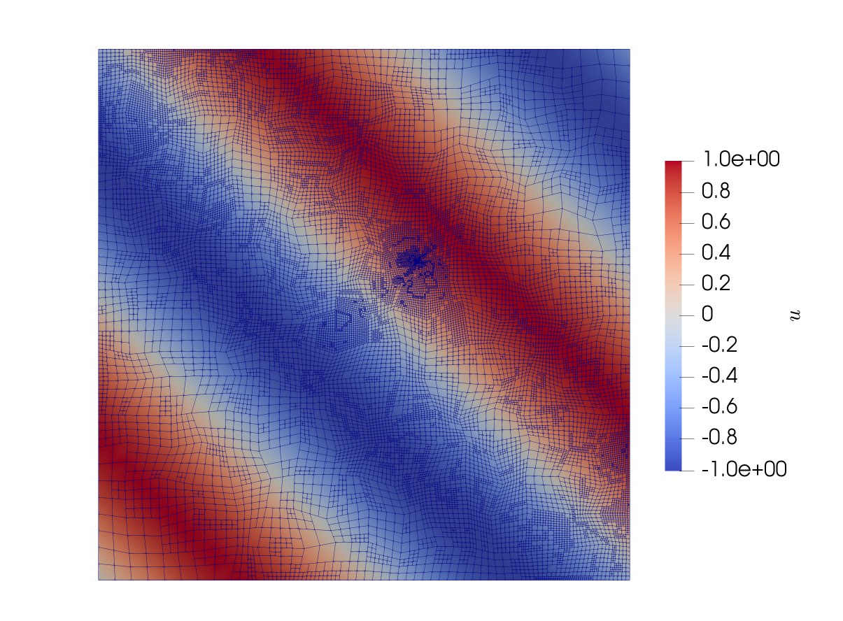
Figure 2: Section 6.2.2, Case 1. Primal solution and mesh after six adaptive refinements.

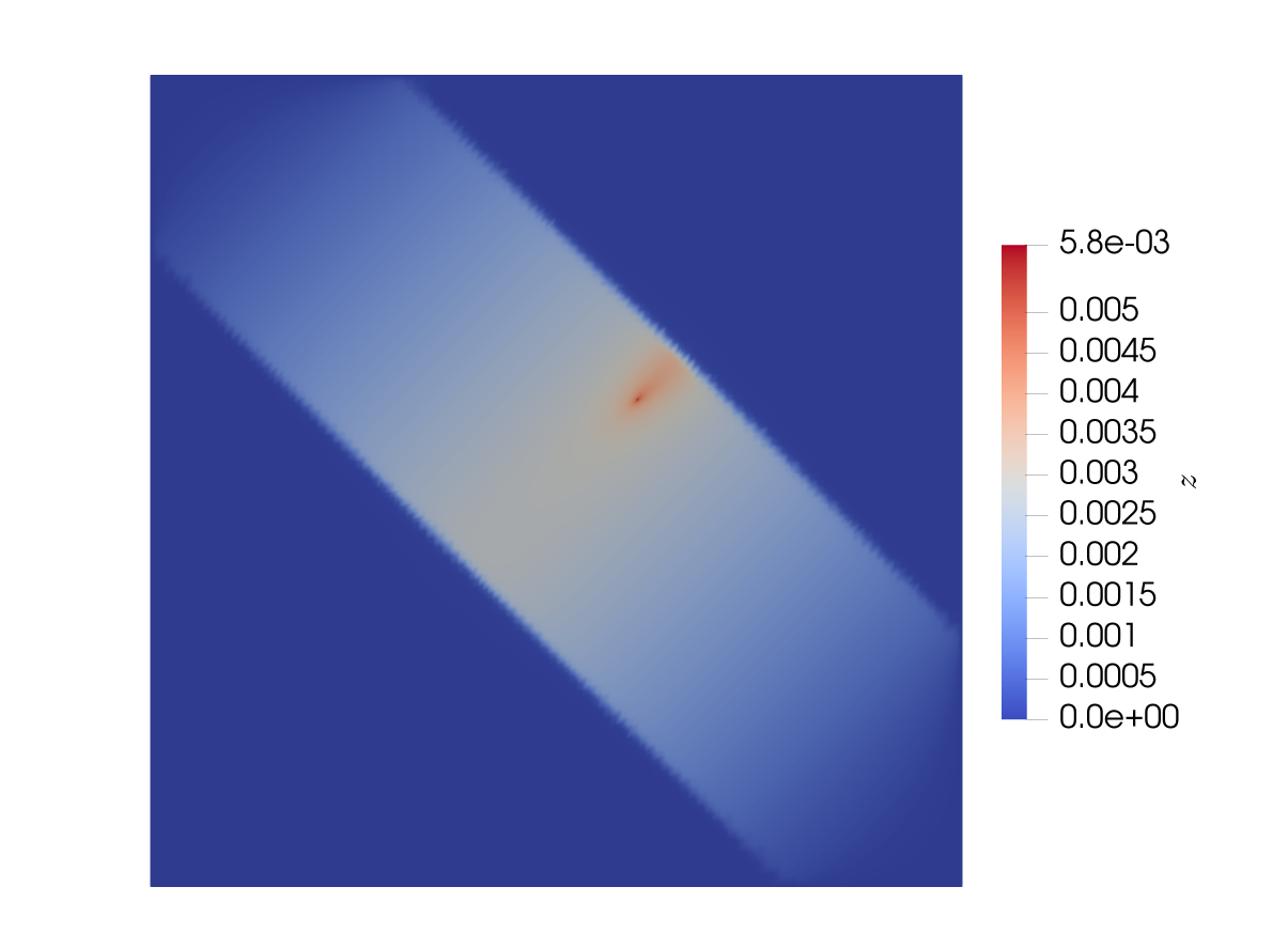
Figure 3: Section 6.2.2, Case 1. Adjoint solution on the mesh as given in Figure 3.

Figure 4: Section 6.2.2, Case 1. Error vs DOFs for $p=5$ and $\varepsilon=0.5$.

Figure 5: Section 6.2.2, Case 2. Error vs DOFs for $p=1.5$ and $\varepsilon=0.5$.

$l$	DOFs	$|J(u)-J(u_{h})|$	$I_{eff}$	$I_{effp}$	$I_{effa}$
1	289	4.24E-03	0.48	0.60	1.56
2	599	5.23E-03	0.80	0.63	0.98
3	1 095	7.72E-04	0.16	0.02	0.34
4	2 418	8.52E-05	1.81	2.58	1.03
5	4 918	1.28E-05	4.92	3.35	6.49
6	10 112	2.64E-05	2.03	1.83	2.22
7	20 068	3.46E-06	5.59	10.33	0.86
8	40 302	1.02E-05	1.66	2.16	1.16
9	79 468	4.45E-06	1.51	1.60	1.43
10	157 272	2.68E-06	1.62	1.68	1.55
11	305 901	1.36E-06	1.32	1.62	1.01
12	602 720	8.52E-07	1.29	1.46	1.12
13	1 157 353	3.40E-07	1.28	1.55	1.01

Table 6: Section 6.2.2, Case 1. Effectivity indices for $p=5$ and $\varepsilon=0.5$.

$l$	DOFs	$|J(u)-J(u_{h})|$	$I_{eff}$	$I_{effp}$	$I_{effa}$
1	289	2.07E-02	0.61	0.47	0.75
2	503	5.55E-03	0.72	0.89	0.55
3	994	2.88E-03	0.89	1.30	0.49
4	2 090	8.55E-04	1.23	1.50	0.96
5	4 233	4.34E-04	1.45	1.90	1.00
6	8 667	1.42E-04	1.34	1.88	0.80
7	17 276	8.14E-05	1.40	2.71	0.09
8	34 846	3.54E-05	1.28	1.75	0.80
9	68 765	1.64E-05	1.36	2.58	0.14
10	136 267	8.59E-06	1.29	2.07	0.51
11	263 508	4.30E-06	1.19	2.20	0.18
12	514 223	2.18E-06	1.22	1.99	0.44
13	988 042	1.01E-06	1.22	2.20	0.24

Table 7: Section 6.2.2, Case 2. Effectivity indices for $p=1.5$ and $\varepsilon=0.5$.

Figure 6: Disturbed initial mesh for Case 1 and Case 2 of Section 6.2.2.

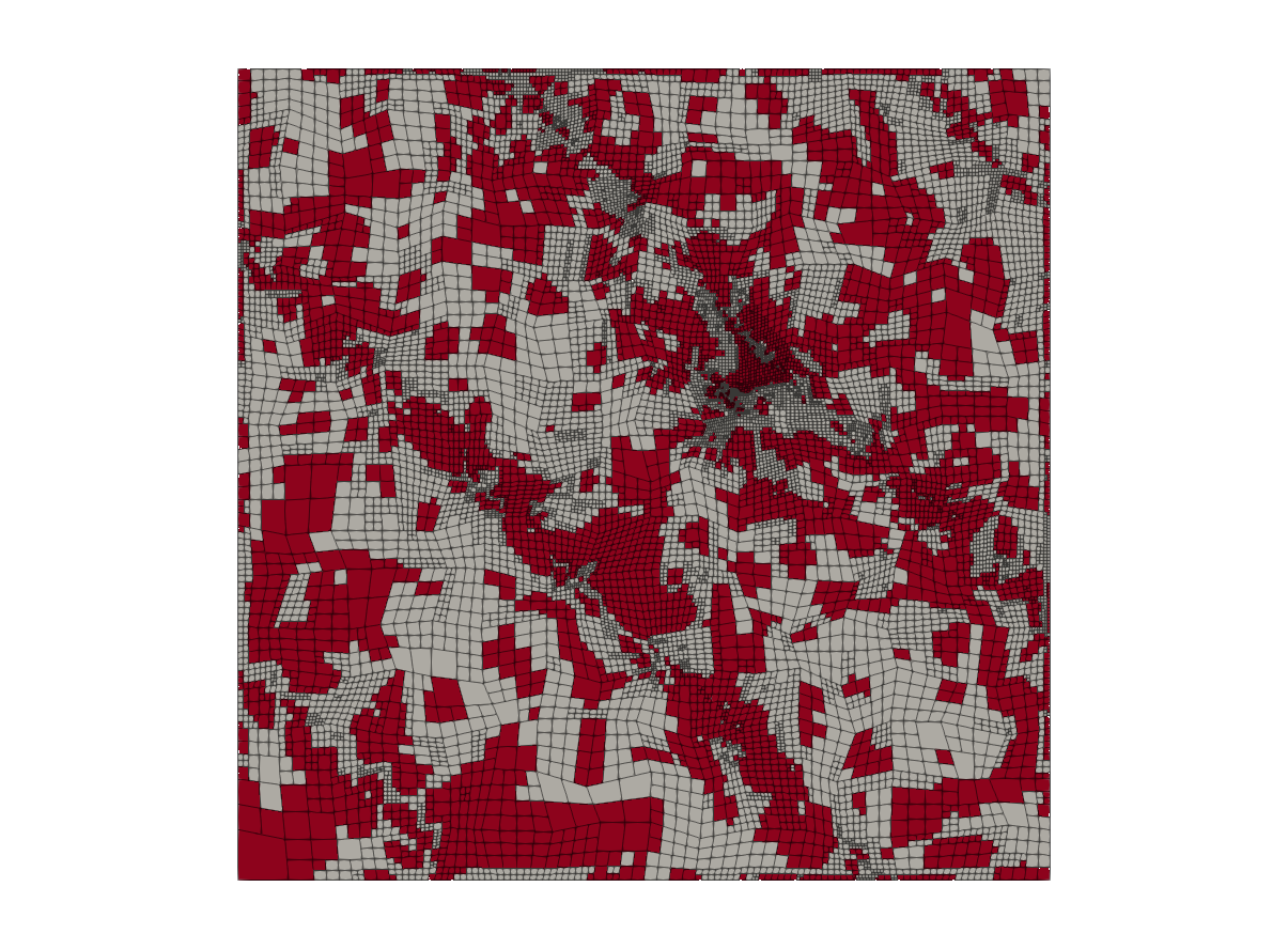
Figure 7: Marked elements (in red) at refinement level $l=7$ for Case 2 of Section 6.2.2.

6.2.3 Low regularity cases

As in Section 6.2.1, we consider homogeneous Dirichlet conditions and $f=1$ as right-hand side for the $p$-Laplace equation (30). However, here both the solution and adjoint solution have low regularity. The initial mesh is given as in Figure 14, which was constructed using the deal.II [6, 5] command cheese. With this data, we have singularities on each of the reentrant corners. Furthermore, in this example, we chose the regularization parameter $\varepsilon$ to be $10^{-10}$, which makes the problem very ill-conditioned (in fact it is practically the original $p$-Laplace problem) where $\nabla u=0$, but it is very close to the unregularized $p$-Laplace problem as in [36] and[23]. We are interested in the following four goal functionals:

$$J_{1}(u):= (1+u(2.9,2.1))(1+u(2.1,2.9)),$$

$$J_{2}(u):= \left(\int_{\Omega}u(x,y)-u(2.5,2.5)\,d(x,y)\right)^{2},$$

$$J_{3}(u):= \int_{(2,3)\times(2,3)}u(x,y)\,d(x,y),$$

$$J_{4}(u):= u(0.6,0.6).$$

These functionals will be combined to $J_{\mathfrak{E}}$ as formulated in (24).
Case 1 ($p=4$, $\varepsilon=10^{-10}$): First we consider a case where $p>2$. The following values, which were computed on a fine grid (8 global refinements, $Q_{c}^{2}$ elements, 22 038 525 DOFs) on the cluster RADON1, are used to compute the reference values:
$\displaystyle\int_{\Omega}u(x,y)\,d(x,y)\approx$ $\displaystyle 4.1285036414\pm 4\times 10^{-5},$ $\displaystyle\int_{(2,3)\times(2,3)}u(x,y)\,d(x,y)\approx$ $\displaystyle 0.31999986649\pm 10^{-5},$ $\displaystyle u(2.9,2.1)\approx$ $\displaystyle 0.16071095234\pm 10^{-5},$ $\displaystyle u(2.9,2.1)\approx$ $\displaystyle 0.16071095234\pm 10^{-5},$ $\displaystyle u(0.6,0.6)\approx$ $\displaystyle 0.35554352679\pm 2\times 10^{-6},$ $\displaystyle u(2.5,2.5)\approx$ $\displaystyle 0.49244705234\pm 4\times 10^{-6}.$ Considering the accuracy of the functional evaluations above, we observe that the relative errors in the functionals $J_{1}$, $J_{2}$, $J_{3}$ and $J_{4}$ are less than $5\times 10^{-5}$. Our algorithm yields the results shown in Table 8. In Figure 8, we can see that the absolute error in the error functional $J_{\mathfrak{E}}$ bounds the relative errors of the functionals $J_{1}$, $J_{2}$, $J_{3}$ and $J_{4}$. Furthermore, we observe that $J_{2}$ is the dominating functional and $J_{1}$ is the one with the smallest error on most refinement levels. Therefore, we compare the convergence of this functionals in Figure 10. For uniform refinement, we obtain an error behavior of approximately $\mathcal{O}(\text{DOFs}^{-\frac{3}{4}})$ for $J_{2}$ and $\mathcal{O}(\text{DOFs}^{-\frac{3}{5}})$ for $J_{1}$, whereas we obtain excellent convergence rates of $\mathcal{O}(\text{DOFs}^{-1})$ for both functionals using our refinement algorithm. We are not aware of a full convergence analysis on adaptive meshes for pointwise estimates for the $p$-Laplacian, but mention two related studies [16] for $p>2$ showing a posteriori estimates for the $W^{1,p}$ norm and [14] with pointwise a priori estimates for the $p$-Laplacian. The bad convergence of $J_{2}$ might result from the fact that the point $(2.5,2.5)$ is the intersection of two lines, where the problem is ill-conditioned, and also leads to a kink in the solution at this point (see Figure 14). This kink is not visible in the case $p=1.33$ (see Figure 14). Comparing the number of Newton steps in Table 9 and Table 10, we observe that the number of Newton steps is less than for Algorithm 2. However, the additional computational cost has to be considered, but we face a problem with nonlinear functionals, several reentrant corners and a very small regularization parameter $\varepsilon=10^{-10}$. Furthermore, these tables also suggest that we should compute both the primal and the adjoint error estimator to obtain a better approximation of the error.

$l$	DOFs	$I_{eff}$	$\left|\frac{J_{1}(u)-J_{1}(u_{h})}{J_{1}(u)}\right|$	$\left|\frac{J_{2}(u)-J_{2}(u_{h})}{J_{2}(u)}\right|$	$\left|\frac{J_{3}(u)-J_{3}(u_{h})}{J_{3}(u)}\right|$	$\left|\frac{J_{4}(u)-J_{4}(u_{h})}{J_{4}(u)}\right|$
1	117	0.63	5.05E-02	3.02E-01	1.10E-01	1.17E-01
2	161	0.53	1.53E-02	5.09E-02	4.94E-02	1.17E-01
3	290	0.84	8.25E-03	4.41E-02	2.14E-02	1.09E-01
4	447	0.81	4.86E-03	5.07E-02	1.53E-02	1.51E-02
5	791	0.96	2.09E-03	3.26E-02	1.12E-02	8.82E-03
6	1 331	1.14	1.37E-03	1.69E-02	8.44E-03	2.40E-03
7	2 541	1.92	1.65E-03	3.37E-03	4.38E-03	1.21E-03
8	4 582	1.38	6.56E-04	3.78E-03	2.43E-03	8.57E-04
9	7 378	1.64	3.14E-04	2.52E-03	1.05E-03	2.06E-04
10	11 772	1.51	2.72E-04	1.73E-03	8.83E-04	3.51E-04
11	20 443	1.87	9.65E-05	5.65E-05	5.24E-04	5.84E-05
12	37 747	1.87	6.09E-05	3.05E-04	2.17E-04	1.20E-04
13	64 316	1.63	2.80E-05	1.30E-04	1.41E-04	4.25E-05
14	104 832	1.44	1.04E-05	1.39E-04	7.18E-05	2.02E-05

Table 8: Section 6.2.3, Case 1. Relative errors for the goal functionals on several refinement levels ($l$) and effectivity index $I_{eff}$ that is computed for $J_{\mathfrak{E}}$ (24).

$l$	DOFs	Error in $J_{\mathfrak{E}}$	$I_{eff}$	$I_{effp}$	$I_{effa}$	Newton steps
1	117	7.43E-01	0.63	0.6	0.65	8
2	161	2.54E-01	0.53	0.27	0.79	2
3	290	1.94E-01	0.84	0.24	1.43	2
4	447	8.40E-02	0.81	0.28	1.34	5
5	791	5.39E-02	0.96	0.48	1.45	4
6	1 331	2.89E-02	1.14	0.24	2.05	1
7	2 541	1.06E-02	1.92	0.02	3.86	3
8	4 582	7.71E-03	1.38	0.41	2.36	4
9	7 378	4.09E-03	1.64	0.74	2.55	2
10	11 772	3.23E-03	1.51	0.7	2.32	4
11	20 443	6.23E-04	1.87	1.06	2.67	2
12	37 747	7.03E-04	1.87	0.66	3.07	6
13	64 316	3.41E-04	1.63	0.39	2.87	4
14	104 832	2.42E-04	1.44	0.5	2.38	3

Table 9: Errors in $J_{\mathfrak{E}}$, effectivity indices and number of Newton steps for $p=4$ and Algorithm 2.

$l$	DOFs	Error in $J_{\mathfrak{E}}$	$I_{eff}$	$I_{effp}$	$I_{effa}$	Newton steps
1	117	7.43E-01	0.63	0.60	0.65	7
2	161	2.58E-01	0.52	0.26	0.79	4
3	290	1.94E-01	0.84	0.24	1.44	4
4	447	8.41E-02	0.81	0.28	1.34	6
5	791	5.40E-02	0.96	0.48	1.45	4
6	1 331	2.70E-02	1.38	0.38	2.39	6
7	2 198	2.02E-02	1.13	0.56	1.70	5
8	4 012	9.07E-03	1.43	0.70	2.16	6
9	6 879	4.02E-03	1.75	0.32	3.18	5
10	11 576	3.27E-03	1.40	0.62	2.19	6
11	20 187	8.20E-04	2.11	0.85	3.37	6
12	38 302	6.77E-04	1.78	0.54	3.02	7
13	64 740	3.12E-04	1.67	0.32	3.02	7
14	105 350	2.46E-04	1.35	0.47	2.22	5

Table 10: Errors in $J_{\mathfrak{E}}$, effectivity indices and number of Newton steps for $p=4$ and Algorithm 2 where $|\mathcal{A}(u^{l,k}_{h})(z^{l,k}_{h})|>10^{-2}\eta_{h}^{l-1}$ is replaced by $\|\mathcal{A}(u_{h}^{l,k})\|_{\ell_{\infty}}>10^{-8}$.

Figure 8: Section 6.2.3, Case 1. Error vs DOFs for $p=4$, $\varepsilon=10^{-10}$.

Figure 9: Section 6.2.3, Case 2. Error vs DOFs for $p=1.33$ and $\varepsilon=10^{-10}$.

Figure 10: Section 6.2.3, Case 1. Error vs DOFs for $p=4$ and $\varepsilon=10^{-10}$.

Figure 11: Section 6.2.3, Case 2. Error vs DOFs for $p=1.33$ and $\varepsilon=10^{-10}$.

Case 2 ($p=1.33$, $\varepsilon=10^{-10}$):
We are interested in the same goal functional as in Case 1 but with $p=1.33$. The following values, which are computed on a fine grid (8 global refinements, $Q_{c}^{2}$ elements, $22\,038\,525$ DOFs) on the cluster RADON1, are used to compute the reference values:
$\displaystyle\int_{\Omega}u(x,y)\,d(x,y)\approx$ $\displaystyle 0.48510099008\pm 4\times 10^{-5},$ $\displaystyle\int_{(2,3)\times(2,3)}u(x,y)\,d(x,y)\approx$ $\displaystyle 0.038058285978\pm 4\times 10^{-6},$ $\displaystyle u(2.9,2.1)\approx$ $\displaystyle 0.034930138311\pm 4\times 10^{-6},$ $\displaystyle u(2.9,2.1)\approx$ $\displaystyle 0.034930138311\pm 4\times 10^{-6},$ $\displaystyle u(0.6,0.6)\approx$ $\displaystyle 0.024478640536\pm 2\times 10^{-6},$ $\displaystyle u(2.5,2.5)\approx$ $\displaystyle 0.039616834482\pm 4\times 10^{-6}.$

Considering again that the accuracy of the functional evaluations is valid, we observe that the relative error of $J_{2}$ is less than $8\times 10^{-4}$ and the relative error of $J_{1},J_{3},J_{4}$ is less than $10^{-4}$. As in Case 1, we compare the relative errors of the functionals in Figure 9. Here we see that the error in $J_{\mathfrak{E}}$ bounds the relative errors. However, we loose control of the single functionals as long as they do not dominate the error, as for $J_{2}$ in Figure 9. In Case 2, $J_{3}$ and $J_{1}$, are these functionals. In the error plot given in Figure 11, we observe that the error approximately behaves like $\mathcal{O}(\text{DOFs}^{-\frac{3}{4}})$ for a uniformly refined mesh, and $\mathcal{O}(\text{DOFs}^{-1})$ for adaptive refinement, as for $p=4$. It turns out that the regions of refinement (except for corner singularities and the point evaluations) have almost a complementary structure for $p=1.33$ and $p=4$ as we can conclude from Figure 17 and Figure 17.

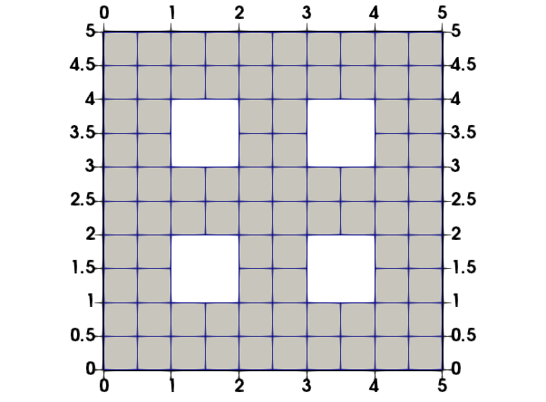
Figure 12: Initial mesh.

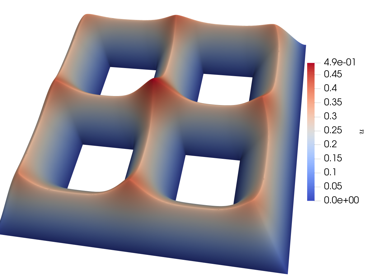
Figure 13: 6.2.3: Solution for $p=4$.

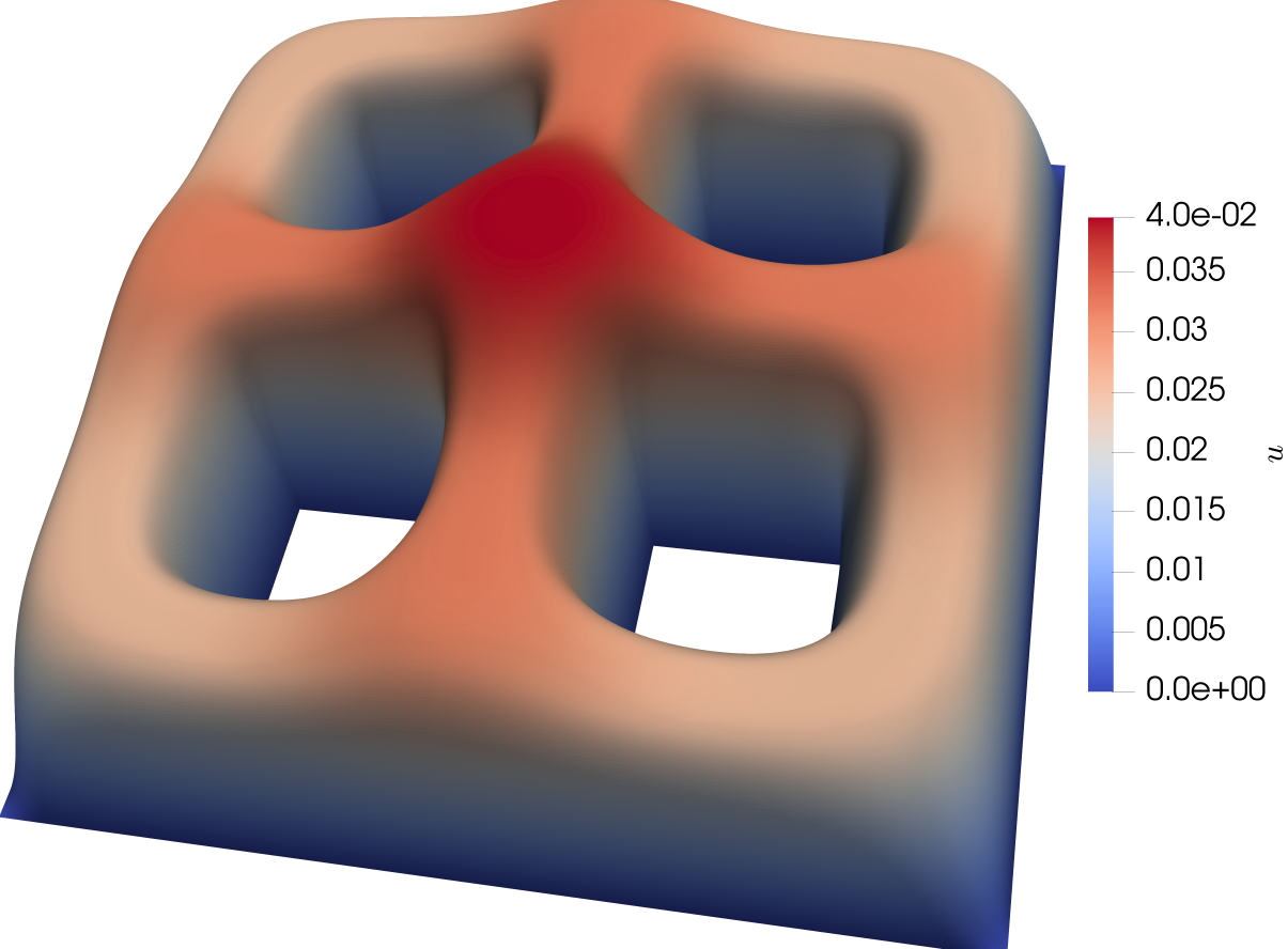
Figure 14: Section 6.2.3: Solution for $p=1.33$.

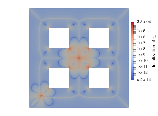
Figure 15: Section 6.2.3: Local error estimator after $6$ uniform refinements for $p=4$.

Figure 16: Section 6.2.3: Mesh after $11$ adaptive refinements for $p=4$ ($37$ $747$ DOFs).

Figure 17: Section 6.2.3: Mesh after $11$ adaptive refinements for $p=1.33$ ($40$ $499$ DOFs).

6.3 Example 2: A quasilinear PDE system

In this second numerical test, we further substantiate our approach for a nonlinear, coupled, PDE system. We consider the following nonlinear boundary value problem: Find $u=(u_{1},u_{2},u_{3})$ such that

$$\begin{aligned} -\Delta u_{1}+u_{2}+u_{3}&=1,\quad\text{in }\Omega,\\ -\Delta u_{2}+g_{1}(1-u_{2})-g_{1}(u_{3})&=0,\quad\text{in }\Omega,\\ -\text{div}(g_{2}(u_{1}+u_{2})\nabla u_{3})+g_{1}(u_{3})-g_{1}(u_{1})&=0,\quad\text{in }\Omega,\end{aligned}$$

is fulfilled in a weak sense, where

$$u_{1}(x,y)=1-u_{2}(x,y)=u_{3}(x,y) =\text{sign($y$)}\sqrt{\sqrt{x^{2}+y^{2}}-x}\qquad\text{on }\Gamma_{D},$$

$$\nabla u_{1}.\vec{n}=\nabla u_{2}.\vec{n}=g_{2}(u_{1}+u_{2})\nabla u_{3}.\vec{n} =0\qquad\text{on }\Gamma_{N}.$$

Here sign denotes the signum function as defined in (18). The functions $g_{1}$ and $g_{2}$ are given by $g_{1}(t):=e^{t}-\text{sin}(t-1)$ and $g_{2}(t):=e^{t^{2}-t}$, respectively. Obviously a solution is given by $u_{1}(x,y)=1-u_{2}(x,y)=u_{3}(x,y)=\text{sign(y)}\sqrt{\sqrt{x^{2}+y^{2}}-x}$ in $\Omega$. The computational domain is a slit domain as in [20, 51, 3] and visualised in Figure 19. The boundary conditions above introduces a discontinuity on the slit-boundary $(-1,0)\times\{0\}$ and consequently a discontinuity in the solution. The construction of this example was motivated by [3, 11]. Let $J_{A},J_{B},J_{C},J_{D},J_{E},J_{F}$ be defined as follows:
$\displaystyle J_{A}(u):=$ $\displaystyle u_{3}(-0.5,0.01),$ $\displaystyle J_{D}(u):=$ $\displaystyle\int_{\Omega}\Phi_{D}(x,y)\cdot u(x,y)\,d(x,y),$ $\displaystyle J_{B}(u)$ $\displaystyle:=u_{1}(-0.01,0.01),$ $\displaystyle J_{E}(u)$ $\displaystyle:=u_{1}(-0.9,-0.9),$ $\displaystyle J_{C}(u):=$ $\displaystyle\int_{\Omega}\Phi_{C}(x,y)\cdot u(x,y)\,d(x,y),$ $\displaystyle J_{F}(u):=$ $\displaystyle u_{2}(-0.9,-0.1),$ where $\Phi_{C}(x,y):=(0,0,\chi_{C}(x,y))$ and

$$\Phi_{D}(x,y):=(-4\chi_{D}(x,y),\frac{2\chi_{D}(x,y)}{1-\text{sign(y)}\sqrt{\sqrt{x^{2}+y^{2}}-x}},4\chi_{D}(x,y)),$$

with

$$\chi_{C}(x,y):=\begin{cases}y-x\quad&x<y\\ 0\quad&x\geq y\end{cases}\quad\mbox{and}\quad\chi_{D}(x,y):=\begin{cases}1\quad&x,y>0\\ 0\quad&\text{else}\end{cases}.$$

We are now interested in the six goal functionals

$$J_{1}(u):= J_{B}(u)J_{D}(u),$$

$$J_{4}(u):= J_{B}(u)J_{E}(u),$$

$$J_{2}(u):= J_{A}(u)J_{C}(u),$$

$$J_{6}(u):= J_{B}^{3}(u)J_{E}(u),$$

$$J_{3}(u):= J_{A}(u)J_{C}(u)J_{F}(u),$$

$$J_{6}(u)= J_{C}(u).$$

For the functional $J_{B}$, we can not expect optimal convergence rates for uniform refinement due to the singularity at the slit tip. Consequently, the same is true for the functionals $J_{1}$, $J_{4}$ and $J_{5}$ as monitored in Figures 21,21 and 23. For uniform refinement, we got a relative error in $J_{1}$ of about $1.409531\times 10^{-2}$ with $3$ $153$ $411$ DOFs as visualized in Figure 21. To achieve a relative error less than $1.409531\times 10^{-2}$ our adaptive algorithm just needs $2$ $538$ DOFs ( $1.042219\times 10^{-2}$ ). If we use a similar number of DOFs ($3$ $021$ $045$), then a relative error of $2.829422\times 10^{-6}$ is achieved. Figures 21, 21 and 23 might also lead to the conclusion that we obtain a convergence rate $\mathcal{O}(\text{DOFs}^{-1})$ for all given functionals, where the functionals for uniform refinement just converge with approximately $\mathcal{O}(\text{DOFs}^{-\frac{1}{2}})$. This means, to obtain a relative error in $J_{1}$ of about $2.829422\times 10^{-6}$ for uniform refinement, we would need approximately $5\times 10^{13}$ DOFs. This would mean just storing the solution would require approximately 400 Terabyte. Therefore, obtaining this accuracy by means of uniform refinement would even be a hard task on the supercomputer Sunway TaihuLight, which is number one the of TOP500 list from November 2017.

We remark that $I_{eff}$, illustrated in Figure 23, has no importance on course meshes since the approximations properties are bad anyway. On finer meshes, we see excellent behavior.

Figure 18: Example 2: The slit domain $\Omega$ with $\Gamma_{D}$ (red) and $\Gamma_{N}$ (blue).

Figure 19: Example 2: Adaptively refined mesh for $J_{\mathfrak{E}}$ after $24$ refinements ($683$ $118$ DOFs).

Figure 20: Example 2: Error vs DOFs.

Figure 21: Example 2: Error vs DOFs.

Figure 22: Example 2: Error vs DOFs.

Figure 23: Example 2: Effectivity of the Error estimators.

7 Conclusions

In this work, we have further developed adaptive schemes for multigoal-oriented a posteriori error estimation and mesh adaptivity. First, we extended the existing methods to nonlinear problems. Second, we combined the estimation of the discretization error with an estimation of the nonlinear iteration error in order to obtain adaptive stopping rules for Newton’s method. In the key Sections 4 and 5, we formulated an abstract framework and its algorithmic realization. In Section 6, these developments were substantiated with several numerical tests. Here, we studied the regularized $p$-Laplace problem and a nonlinear, coupled PDE system. Our findings demonstrate the performance of the algorithms and specifically that the adjoint part of the error estimator, which is often neglected in the literature because of its higher computational cost, must be taken into account in order to achieve good effectivity indices. In view of the geometric singularities, nonlinearities in both the PDE and the goal functionals, our results show excellent performance of our algorithms.

8 Acknowledgments

This work has been supported by the Austrian Science Fund (FWF) under the grant P 29181 ‘Goal-Oriented Error Control for Phase-Field Fracture Coupled to Multiphysics Problems’. The first author thanks the Doctoral Program on Computational Mathematics at JKU Linz the Upper Austrian Goverment for the support when starting the preparation of this work. The third author was supported by the Doctoral Program on Computational Mathematics during his visit at the Johannes Kepler University Linz in March 2018.

References

- [1] R. Adams and J. Fournier. Sobolev Spaces. Pure and Applied Mathematics. Elsevier Science, 2003.
- [2] M. Ainsworth and J. T. Oden. A posteriori error estimation in finite element analysis. Pure and Applied Mathematics. John Wiley & Sons, New York, 2000.
- [3] J. Andersson and H. Mikayelyan. The asymptotics of the curvature of the free discontinuity set near the cracktip for the minimizers of the Mumford-Shah functional in the plain. a revision. arXiv: 1205.5328v2, 2015.
- [4] D. N. Arnold, D. Boffi, and R. S. Falk. Approximation by quadrilateral finite elements. Math. Comp., 71(239):909–922, 2002.
- [5] W. Bangerth, D. Davydov, T. Heister, L. Heltai, G. Kanschat, M. Kronbichler, M. Maier, B. Turcksin, and D. Wells. The deal.II library, version 8.4. J. Numer. Math., 24(3):135–141, 2016.
- [6] W. Bangerth, R. Hartmann, and G. Kanschat. deal.II – a general purpose object oriented finite element library. ACM Trans. Math. Softw., 33(4):24/1–24/27, 2007.
- [7] W. Bangerth and R. Rannacher. Adaptive Finite Element Methods for Differential Equations. Birkhäuser Verlag, Boston, 2003.
- [8] R. Becker, C. Johnson, and R. Rannacher. Adaptive error control for multigrid finite element methods. Computing, 55(4):271–288, 1995.
- [9] R. Becker and R. Rannacher. Weighted a posteriori error control in FE methods. In e. a. H. G. Bock, editor, ENUMATH’97. World Sci. Publ., Singapore, 1995.
- [10] R. Becker and R. Rannacher. An optimal control approach to a posteriori error estimation in finite element methods. Acta Numer., 10:1–102, 2001.
- [11] A. Bonnet and G. David. Cracktip is a global Mumford-Shah minimizer. Asterisque No. 274, 2001.
- [12] M. Braack and A. Ern. A posteriori control of modeling errors and discretization errors. Multiscale Model. Simul., 1(2):221–238, 2003.
- [13] D. Braess. Finite Elemente; Theorie, schnelle Löser und Anwendungen in der Elastizitätstheorie. Springer-Verlag Berlin Heidelberg, 4., überarbeitete und erweiterte Auflage edition, 2007.
- [14] D. Breit, A. Cianchi, L. Diening, T. Kuusi, and S. Schwarzacher. The -Laplace system with right-hand side in divergence form: inner and up to the boundary pointwise estimates. Nonlinear Anal., 153:200–212, 2017.
- [15] G. F. Carey and J. T. Oden. Finite Elements. Volume III. Compuational Aspects. The Texas Finite Element Series, Prentice-Hall, Inc., Englewood Cliffs, 1984.
- [16] C. Carstensen and R. Klose. A posteriori finite element error control for the -Laplace problem. SIAM J. Sci. Comput., 25(3):792–814, 2003.
- [17] P. G. Ciarlet. Finite Element Method for Elliptic Problems. Society for Industrial and Applied Mathematics, Philadelphia, PA, USA, 2002.
- [18] T. A. Davis. Algorithm 832: Umfpack v4.3—an unsymmetric-pattern multifrontal method. ACM Trans. Math. Softw., 30(2):196–199, June 2004.
- [19] L. Diening and M. Růžička. Interpolation operators in Orlicz-Sobolev spaces. Numer. Math., 107(1):107–129, 2007.
- [20] B. Endtmayer and T. Wick. A Partition-of-Unity Dual-Weighted Residual Approach for Multi-Objective Goal Functional Error Estimation Applied to Elliptic Problems. Comput. Methods Appl. Math., 17(4):575–599, 2017.
- [21] A. Ern and M. Vohralík. Adaptive inexact Newton methods with a posteriori stopping criteria for nonlinear diffusion PDEs. SIAM J. Sci. Comput., 35(4):A1761–A1791, 2013.
- [22] C. Giannelli, B. Jüttler, and H. Speleers. THB-splines: the truncated basis for hierarchical splines. Comput. Aided Geom. Design, 29(7):485–498, 2012.
- [23] R. Glowinski and A. Marroco. Sur l’approximation, par éléments finis d’ordre un, et la résolution, par pénalisation-dualité d’une classe de problèmes de Dirichlet non linéaires. ESAIM: Mathematical Modelling and Numerical Analysis - Modélisation Mathématique et Analyse Numérique, 9(R2):41–76, 1975.
- [24] W. Hackbusch. Multi-Grid Methods and Applications. Springer, 2003.
- [25] W. Han. A Posteriori Error Analysis Via Duality Theory : With Applications in Modeling and Numerical Approximations. Springer, 2005.
- [26] R. Hartmann. Multitarget error estimation and adaptivity in aerodynamic flow simulations. SIAM J. Sci. Comput., 31(1):708–731, 2008.
- [27] R. Hartmann and P. Houston. Goal-oriented a posteriori error estimation for multiple target functionals. In Hyperbolic problems: theory, numerics, applications, pages 579–588. Springer, Berlin, 2003.
- [28] A. Hirn. Finite element approximation of singular power-law systems. Math. Comp., 82(283):1247–1268, 2013.
- [29] P. Houston, B. Senior, and E. Süli. -discontinuous Galerkin finite element methods for hyperbolic problems: error analysis and adaptivity. Internat. J. Numer. Methods Fluids, 40(1-2):153–169, 2002. ICFD Conference on Numerical Methods for Fluid Dynamics (Oxford, 2001).
- [30] T. J. R. Hughes, J. A. Cottrell, and Y. Bazilevs. Isogeometric analysis: CAD, finite elements, NURBS, exact geometry and mesh refinement. Comput. Methods Appl. Mech. Engrg., 194:4135–4195, 2005.
- [31] K. Kergrene, S. Prudhomme, L. Chamoin, and M. Laforest. A new goal-oriented formulation of the finite element method. Comput. Methods Appl. Mech. Engrg., 327:256–276, 2017.
- [32] M. A. Khamsi and W. A. Kirk. An introduction to metric spaces and fixed point theory. Pure and Applied Mathematics (New York). Wiley-Interscience, New York, 2001.
- [33] S. K. Kleiss and S. K. Tomar. Guaranteed and sharp a posteriori error estimates in isogeometric analysis. Comput. Math. Appl., 70(3):167–190, 2015.
- [34] U. Langer, S. Matculevich, and S. Repin. Functional type error control for stabilised space-time iga approximations to parabolic problems. In I. Lirkov and S. Margenov, editors, Large-Scale Scientific Computing (LSSC 2017), Lecture Notes in Computer Science (LNCS), pages 57–66. Springer-Verlag, 2017.
- [35] U. Langer, S. Matculevich, and S. Repin. Guaranteed error control bounds for the stabilised space-time iga approximations to parabolic problem. Technical Report arXiv:1712.06017 [math.NA], 2017.
- [36] P. Lindqvist. Notes on the -Laplace equation, volume 102 of Report. University of Jyväskylä Department of Mathematics and Statistics. University of Jyväskylä, Jyväskylä, 2006.
- [37] D. Meidner, R. Rannacher, and J. Vihharev. Goal-oriented error control of the iterative solution of finite element equations. J. Numer. Math., 17(2):143–172, 2009.
- [38] P. Neittaanmäki and S. Repin. Reliable Methods for Computer Simulation: Error Control and Posteriori Estimates. Elsevier, Amsterdam, 2004.
- [39] D. Pardo. Multigoal-oriented adaptivity for hp-finite element methods. Procedia Computer Science, 1(1):1953 – 1961, 2010.
- [40] R. Rannacher and J. Vihharev. Adaptive finite element analysis of nonlinear problems: balancing of discretization and iteration errors. J. Numer. Math., 21(1):23–61, 2013.
- [41] R. Rannacher, A. Westenberger, and W. Wollner. Adaptive finite element solution of eigenvalue problems: balancing of discretization and iteration error. J. Numer. Math., 18(4):303–327, 2010.
- [42] S. Repin. A posteriori estimates for partial differential equations, volume 4 of Radon Series on Computational and Applied Mathematics. Walter de Gruyter GmbH & Co. KG, Berlin, 2008.
- [43] A. Reusken. Convergence of the multigrid full approximation scheme for a class of elliptic mildly nonlinear boundary value problems. Numer. Math., 52(3):251–277, 1988.
- [44] T. Richter and T. Wick. Variational localizations of the dual weighted residual estimator. J. Comput. Appl. Math., 279:192–208, 2015.
- [45] W. Sierpinski. General topology. Mathematical Expositions, No. 7. University of Toronto Press, Toronto, 1952. Translated by C. Cecilia Krieger.
- [46] P. Stolfo, A. Rademacher, and A. Schröder. Dual weighted residual error estimation for the finite cell method. Technical report, Fakultät für Mathematik, TU Dortmund, Sept. 2017. Ergebnisberichte des Instituts für Angewandte Mathematik, Nummer 576.
- [47] I. Toulopoulos and T. Wick. Numerical methods for power-law diffusion problems. SIAM J. Sci. Comput., 39(3):A681–A710, 2017.
- [48] E. H. van Brummelen, S. Zhuk, and G. J. van Zwieten. Worst-case multi-objective error estimation and adaptivity. Comput. Methods Appl. Mech. Engrg., 313:723–743, 2017.
- [49] R. Verfürth. A Review of A Posteriori Error Estimation and Adaptive Mesh-Refinement Techniques. Wiley-Teubner, New York-Stuttgart, 1996.
- [50] S. Weisser and T. Wick. The dual-weighted residual estimator realized on polygonal meshes. Comput. Methods Appl. Math. Published Online: 2017-11-12, DOI: https://doi.org/10.1515/cmam-2017-0046.
- [51] T. Wick. Goal functional evaluations for phase-field fracture using PU-based DWR mesh adaptivity. Comput. Mech., 57(6):1017–1035, 2016.