Relativistic full-configuration-interaction calculations of magic wavelengths for the $2\,^{3}S_{1}\rightarrow 2\,^{1}S_{0}$ transition of helium isotopes

Abstract

A large-scale full-configuration-interaction calculation based on Dirac-Coulomb-Breit (DCB) Hamiltonian is performed for the $2\,^{1}S_{0}$ and $2\,^{3}S_{1}$ states of helium. The operators of the normal and specific mass shifts are directly included in the DCB framework to take the finite nuclear mass correction into account. High-accuracy energies and matrix elements involved n (the main quantum number) up to 13 are obtained from one diagonalization of Hamiltonian. The dynamic dipole polarizabilities are calculated by using the sum rule of intermediate states. And a series of magic wavelengths with QED and hyperfine effects included for the $2\,^{3}S_{1}\rightarrow 2\,^{1}S_{0}$ transition of helium are identified. In addition, the high-order Ac Stark shift determined by the dynamic hyperpolarizabilities at the magic wavelengths are also evaluated. Since the most promising magic wavelength for application in experiment is 319.8 nm, the high-accuracy magic wavelength of 319.815 3(6) nm of ⁴He is in good agreement with recent measurement value of 319.815 92(15) nm [Nature Physics (2018)/arXiv:1804.06693], and present magic wavelength of 319.830 2(7) nm for ³He would provide theoretical support for experimental designing an optical dipole trap to precisely determine the nuclear charge radius of helium in future.

The long-term outstanding proton radius puzzle causes great interest in recent years Pohl et al. (2010); Antognini et al. (2013); Mohr et al. (2016). So far there has not been a satisfying explanation for the discrepancy of 5.6$\sigma$ in the proton size derived from muonic hydrogen Lamb shift measurements Pohl et al. (2010); Antognini et al. (2013) and the accepted CODATA value Mohr et al. (2016). Research in this field has expanded to measurements of the 2$S$-4$P$ transition energy in hydrogen Beyer et al. (2017), transition energies between circular Rydberg states in heavy-H-like ions Tan et al. (2011), and the 1$S$-2$S$ transition energy in muonic helium ions Antognini et al. (2011). In order to help solve the proton size puzzle, the measurement of high-precision spectroscopy in helium isotopes has become an additional contribution to this field van Rooij et al. (2011); van Leeuwen and Vassen (2006); Shiner et al. (1995); Morton et al. (2006a); Pastor et al. (2004, 2012). However, the nuclear charge radius difference determined from the $2\,^{3}S\rightarrow 2\,^{1}S$ and $2\,^{3}S\rightarrow 2\,^{3}P$ transitions of helium disagrees by 4$\sigma$ van Rooij et al. (2011); van Leeuwen and Vassen (2006); Shiner et al. (1995); Morton et al. (2006a); Pastor et al. (2004, 2012). Even combined with the recent theoretical investigations Pachucki and Yerokhin (2015); Patkóš et al. (2016, 2017), where the higher-order recoil corrections are taken into account, the 4$\sigma$ discrepancy does still exist and remains unexplained by any missed corrections in existing theoretical predictions. So this discrepancy calls for the verification of the experimental transition frequencies by independent measurements.

For the $2\,^{3}S\rightarrow 2\,^{3}P$ transition frequency of helium, recently, the frequency measurement of ⁴He is achieved to $5.1\times 10^{-12}$ Zheng et al. (2017), which is more accurate than the early results of Refs. Pastor et al. (2004, 2006, 2012). But it’s interesting that applying the $2\,^{3}S\rightarrow 2\,^{3}P$ transition frequency of $\,{}^{3}$He of Ref. Pastor et al. (2012) into Ref. Zheng et al. (2017), the resulting nuclear charge radii difference agrees well with the value derived from the $2\,^{3}S\rightarrow 2\,^{1}S$ transition van Rooij et al. (2011) but differs with the measurement of $2\,^{3}S\rightarrow 2\,^{3}P$ transition Shiner et al. (1995). This deviation indicates that further independent measurement of the $2\,^{3}S\rightarrow 2\,^{3}P$ transition for ³He is urgently needed.

For the $2\,^{3}S\rightarrow 2\,^{1}S$ transition frequency of helium, one of the main systematic uncertainty of previous measurement van Rooij et al. (2011) comes from Ac Stark shift. Implementation of a magic wavelength trap can solve this problem in many high-precision measurements Kim et al. (2017); Campbell et al. (2017). Recently, Notermans et al. obtain the magic wavelengths of He($2\,^{3}S\rightarrow 2\,^{1}S$) with use of available energies and Einstein A coefficients Notermans et al. (2014). The accuracy of their values are limited by extrapolated contributions from continuums.

Since the dynamic dipole polarizability at the 319.8 nm magic wavelength is large enough to provide sufficient trap depth at reasonable laser powers while the scattering lifetime is accepted, the 319.8 nm magic wavelength is proposed to design a optical dipole trap (ODT) to eliminate the Ac Stark shift Notermans et al. (2014). In order to determine the nuclear charge radius difference with a precision comparable to the muonic helium ion, Vassen et al. aim to measure the $2\,^{3}S\rightarrow 2\,^{1}S$ transition with sub-kHz precision. At this level of precision, the ab-initio calculation for the magic wavelengths of helium isotopes are required.

In this paper, we improve the previous relativistic configuration interaction (RCI) method Zhang et al. (2016) by adding the mass shift (MS) operators directly into the Dirac-Coulomb-Breit (DCB) Hamiltonian. Then we perform a large-scale full-configuration-interaction calculation of the dynamic dipole polarizabilities for the $2\,^{3}S$ and $2\,^{1}S$ states of helium. QED corrections to the dynamic dipole polarizabilities are approximate by perturbation calculations. A series of magic wavelengths for the $2\,^{3}S_{1}\rightarrow 2\,^{1}S_{0}$ transition are accurately identified according to the dynamic polarizabilities. In addition, we also carry out a non-relativistic calculations of dynamic polarizabilities and hyperpolarizabilities of helium by using the newly developed Hylleraas-B-spline method Yang et al. (2017). Present magic wavelengths from two different theoretical methods are in good agreement. Specially, the accurate magic wavelengths of 319.815 3(6) nm and 319.830 2(7) nm are recommended for the $2\,^{3}S_{1}(M_{J}=\pm 1)\rightarrow 2\,^{1}S_{0}$ transition of ⁴He and ³He, respectively.

The DCB Hamiltonian with mass shift operator included for the two-electron atomic system is written as

$$H=\sum\limits_{i=1}^{2}\left[c\bm{\alpha}_{i}\cdot\bm{p}_{i}+\beta m_{e}c^{2}-\dfrac{Z}{r_{i}}\right]+\dfrac{1}{r_{12}}-\dfrac{1}{2r_{12}}\big{[}\bm{\alpha}_{1}\cdot\bm{\alpha}_{2}+\left(\bm{\alpha}_{1}\cdot\hat{\bm{r}}_{12}\right)\left(\bm{\alpha}_{2}\cdot\hat{\bm{r}}_{12}\right)\big{]}+H_{MS}\,$$ (1)

where $c=137.035999074$ is the speed of light Mohr et al. (2012), $Z$ is the nuclear charge, $\beta$ is the $4\times 4$ Dirac matrix, $m_{e}=1$ is the electron mass, $\bm{\alpha}_{i}$ and $\bm{p}_{i}$ are respectively the Dirac matrix and the momentum operator for the $i$-th electron, $\hat{\bm{r}}_{12}$ is the unit vector of the electron-electron distance $\bm{r}_{12}$, and the MS operator $H_{MS}$ includes the leading term of normal and specific mass shift (NMS, SMS) operators,

$$H_{MS}=H_{NMS}+H_{SMS}=\sum\limits_{i=1}^{2}\dfrac{\bm{p}_{i}^{2}}{2m_{0}}+\dfrac{\bm{p}_{1}\cdot\bm{p}_{2}}{m_{0}}\,,$$ (2)

where $m_{0}=7294.2995361\,m_{e}$ and $m_{0}=5495.8852754\,m_{e}$ Mohr et al. (2012) are the nuclear mass for ⁴He and ³He, respectively. The wave function $\psi(JM_{J})$ for a state with angular momentum $\left(J,M_{J}\right)$ is expanded as a linear combination of the configuration-state wave functions $\phi_{ij}(JM_{J})$, which are constructed by the single-electron wave functions Zhang et al. (2016). Using the Notre Dame basis sets Johnson et al. (1988); Beloy and Derevianko (2008) of B-spline functions, the single-electron wave functions are obtained by solving the single-electron Dirac equation.

The non-relativistic Hamiltonian for the infinite nuclear mass of helium is solved with Hylleraas-B-spline basis set Yang et al. (2017),

$$\phi_{ij\ell_{1}\ell_{2}}\left(LM_{L}\right) = B_{i}^{k}(r_{1})B_{j}^{k}(r_{2})r_{12}^{c}Y_{\ell_{1}\ell_{2}}^{LM_{L}}\left(\hat{r}_{1},\hat{r}_{2}\right)$$ (3)

$$\pm\,exchange\,,$$

where $L$ and $M_{L}$ are the total orbital and magnetic quantum numbers, respectively, $Y_{\ell_{1}\ell_{2}}^{LM_{L}}\left(\hat{r}_{1},\hat{r}_{2}\right)$ is the coupled spherical harmornic function, and $c=0\,,1$.

The dynamic dipole polarizability of the magnetic sublevel $|N_{g}J_{g}M_{J_{g}}\rangle$ under linear polarized light with laser frequency $\omega$ is

$$\alpha_{1}(\omega)=\alpha_{1}^{S}(\omega)+\dfrac{3M_{J_{g}}^{2}-J_{g}(J_{g}+1)}{J_{g}(2J_{g}-1)}\alpha_{1}^{T}(\omega)\,,$$ (4)

where $\alpha_{1}^{S}(\omega)$ and $\alpha_{1}^{T}(\omega)$ are the scalar and tensor dipole polarizabilities, respectively, which can be expressed as the summation over all intermediate states,

$$\alpha_{1}^{S}(\omega)=\sum_{n\neq g}\dfrac{f_{gn}^{(1)}}{(\Delta E_{gn})^{2}-\omega^{2}}\,,$$ (5)

$$\alpha_{1}^{T}(\omega)=\sum_{n\neq g}(-1)^{J_{g}+J_{n}}\sqrt{\dfrac{30(2J_{g}+1)J_{g}(2J_{g}-1)}{(2J_{g}+3)(J_{g}+1)}}\left\{\begin{array}[]{ccc}1&1&2\\ J_{g}&J_{g}&J_{n}\\ \end{array}\right\}\dfrac{f_{gn}^{(1)}}{(\Delta E_{gn})^{2}-\omega^{2}}\,,$$ (8)

with $f_{gn}^{(1)}$ is the dipole oscillator strength,

$$f_{gn}^{(1)}=\dfrac{2|\langle N_{g}J_{g}\|T_{1}\|N_{n}J_{n}\rangle|^{2}\Delta E_{gn}}{3(2J_{g}+1)}\,,$$ (9)

where $\triangle E_{gn}=E_{n}-E_{g}$ is transition energy between the initial state $|N_{g}J_{g}\rangle$ and the intermediate state $|N_{n}J_{n}\rangle$, and $T_{1}$ is the dipole transition operator. The nonrelativistic polarizabilities are obtained by replacing the quantum number $J$ with $L$ in Eqs.(4)- (9).

The QED corrections to dynamic dipole polarizabilities are calculated by the perturbation theory Pachucki and Sapirstein (2000) using energies and wavefunctions obtained from non-relativistic configuration interaction (NRCI) method Zhang et al. (2015),

$$\delta\alpha_{1}^{QED}(\omega) = 2\Bigg{[}\sum\limits_{n}\dfrac{\langle g|T_{1}|n\rangle\langle n|T_{1}|g\rangle\langle g|\delta H_{QED}|g\rangle[(E_{n}-E_{g})^{2}+\omega^{2}]}{[(E_{n}-E_{g})^{2}-\omega^{2}]^{2}}-2\sum\limits_{nm}\dfrac{\langle g|T_{1}|n\rangle\langle n|T_{1}|m\rangle\langle m|\delta H_{QED}|g\rangle(E_{n}-E_{g})}{[(E_{n}-E_{g})^{2}-\omega^{2}](E_{m}-E_{g})}$$ (10)

$$- \sum\limits_{nm}\dfrac{\langle g|T_{1}|n\rangle\langle n|\delta H_{QED}|m\rangle\langle m|T_{1}|g\rangle[(E_{n}-E_{g})(E_{m}-E_{g})+\omega^{2}]}{[(E_{n}-E_{g})^{2}-\omega^{2}][(E_{m}-E_{g})^{2}-\omega^{2}]}\Bigg{]}\,$$

where $|g\rangle$ is the initial state, $|n\rangle$ and $|m\rangle$ represent intermediate states, and $\delta H_{QED}$ is the QED operator. The expansion of $\delta H_{QED}$ Yerokhin and Pachucki (2010) to the leading order of $\alpha^{3}$ is adopted in this work,

$$H_{QED}^{(3)}\simeq\frac{4Z\alpha^{3}}{3}\left\{\dfrac{19}{30}+\ln\big{[}(Z\alpha)^{-2}\big{]}-\ln\big{(}\frac{k_{0}}{Z^{2}}\big{)}\right\}\big{[}\delta^{3}({\mathbb{r}}_{1})+\delta^{3}({\mathbb{r}}_{2})\big{]}+O({\mathbb{r}}_{12})\,,$$ (11)

where $\ln k_{0}$ is the Bethe logarithm, and $O({\mathbb{r}}_{12})$ represents remaining term connected with ${\mathbb{r}}_{12}$. We use $\ln k_{0}=$4.364 036 82(1) and 4.366 412 72(7) Drake and Goldman (1999) for the $2\,^{3}S_{1}$ and $2\,^{1}S_{0}$ states, respectively. Since $O({\mathbb{r}}_{12})$ contributes $-5.2\times 10^{-8}$ a.u. and $-5.6\times 10^{-9}$ a.u. to the energies of $2\,^{1}S_{0}$ and $2\,^{3}S_{1}$ states of helium, respectively, which is three and four orders of magnitude smaller than $1.66\times 10^{-5}$ a.u. and $1.67\times 10^{-5}$ a.u. from the first term of Eq.(11). So in this work, the QED correction to the magic wavelengths is calculated by omitting the $O({\mathbb{r}}_{12})$ contributions.

The nonrelativistic dynamic hyperpolarizability for $S$ state is

$$\gamma_{0}(\omega)=\frac{128\pi^{2}}{3}\big{[}\frac{1}{9}\mathcal{T}(1,0,1,\omega)+\frac{2}{45}\mathcal{T}(1,2,1,\omega)\big{]}\,,$$ (12)

where $\mathcal{T}(L_{a},L_{b},L_{c},\omega)$ is written as

$$\mathcal{T}(L_{a},L_{b},L_{c},\omega) = \sum_{mnk}\frac{\langle N_{g}L_{g}\|T_{1}\|mL_{a}\rangle\langle mL_{a}\|T_{1}\|nL_{b}\rangle\langle nL_{b}\|T_{1}\|kL_{c}\rangle\langle kL_{c}\|T_{1}\|N_{g}L_{g}\rangle}{(\Delta E_{mg}-\omega)\Delta E_{ng}(\Delta E_{kg}-\omega)}$$ (13)

$$- \delta_{L_{b},L_{g}}\sum_{m}\frac{|\langle N_{g}L_{g}\|T_{1}\|mL_{a}\rangle|^{2}}{(\Delta E_{mg}-\omega)}\sum_{k}\frac{|\langle N_{g}L_{g}\|T_{1}\|kL_{c}\rangle|^{2}}{(\Delta E_{kg}-\omega)^{2}}\,.$$

Compared with the dynamic dipole polarizabilities, the accurate calculation of the dynamic hyperpolarizabilities is much more challenging, since the formula involves three summations over different intermediated states, which means the calculation of hyperpolarizability depends on the completeness of the energy spectrum of more intermediate states.

The magic wavelengths of the $2\,^{3}S\rightarrow 2\,^{1}S$ transition are determined from making the dynamic dipole polarizabilities of the $2\,^{1}S_{0}$ and $2\,^{3}S_{1}$ states equally. The accuracy of magic wavelengths depends on accurate energies and wavefunctions of initial and intermediate states. The high-precision B-spline RCI method was very successful in accurate calculation of atomic polarizabilities for the triplet $2\,^{3}S_{1}$ state of helium Zhang et al. (2016). However, for the magic wavelengths around 320 nm of interest in the present work, it’s clearly seen from Fig. 1, they are located at the edge of the $2\,^{1}S_{0}\rightarrow 10\,^{1}P_{1}$, $2\,^{1}S_{0}\rightarrow 11\,^{1}P_{1}$, and $2\,^{1}S_{0}\rightarrow 12\,^{1}P_{1}$ resonance transitions. The accurate determination of these magic wavelengths requires construction of sufficient configurations in an appropriate box size to make sure that all transition energies from the $2\,^{1}S_{0}$ state to the $10\,^{1}P_{1}$, $11\,^{1}P_{1}$, and $12\,^{1}P_{1}$ Rydberg states are accurate. This is a biggest challenge for our RCI calculation.

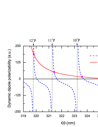
Figure 1: (Color online) Dynamic dipole polarizabilities (in a.u.) of helium for the photon energy 319 nm $\leq\omega\leq$ 326 nm. The solid red line and the dashed blue line represent the dynamic polarizabilities for $2\,^{3}S_{1}(M_{J}=\pm 1)$ and $2\,^{1}S_{0}$ states, respectively. The crossing points marked as solid magenta circle are the magic wavelengths. The vertical lines are the resonance transition positions, and the black line denotes a horizontal line.

We optimize our RCI program by using OpenMP parallel and block calculations, which overcomes the problem of time consuming and large memory required in calculating the electron-electron Coulomb and Breit interaction integrals. Extensive tests of the numerical stability for energies, matrix elements, polarizabilities, and magic wavelengths of helium are carried out.

Table 1: Energy (in a.u.) test of the $2\,^{1}S_{0}$ and $12\,^{1}P_{1}$ states of ⁴He. $N$ is the number of B-spline, $R_{0}$ is the box size, and $\ell_{max}$ presents the number of partial-wave.

	$2\,^{1}S_{0}$		$12\,^{1}P_{1}$
$\ell_{max}$	$(N,R_{0})$=(45,100)	$(N,R_{0})$=(50,600)	$(N,R_{0})$=(50,600)
7	$-$2.145 783 68	$-$2.145 782 91	$-$2.003 297 046
8	$-$2.145 784 58	$-$2.145 783 74	$-$2.003 297 053
9	$-$2.145 785 15	$-$2.145 784 25	$-$2.003 297 057
10	$-$2.145 785 53	$-$2.145 784 58	$-$2.003 297 059
15	$-$2.145 786 27	$-$2.145 785 21	$-$2.003 297 063
Extrap.	$-$2.145 786(1)	$-$2.145 785(1)	$-$2.003 297 06(1)

Table 2: Comparison of present RCI energies (in a.u.) for some selective $n\,^{1}P_{1}\,(n\leq 13)$ states of ⁴He and ³He. The numbers in parentheses are computational uncertainties.

State	4He
	RCI	Hylleraas Drake (2006)
$2\,^{1}P_{1}$	$-$2.123 650 17(2)	$-$2.123 654 51
$3\,^{1}P_{1}$	$-$2.054 968 56(2)	$-$2.054 970 17
$4\,^{1}P_{1}$	$-$2.030 896 59(2)	$-$2.030 897 47
$5\,^{1}P_{1}$	$-$2.019 734 98(2)	$-$2.019 735 59
$6\,^{1}P_{1}$	$-$2.013 664 02(2)	$-$2.013 664 52
$7\,^{1}P_{1}$	$-$2.009 999 98(2)	$-$2.010 000 41
$8\,^{1}P_{1}$	$-$2.007 620 18(2)	$-$2.007 620 57
$9\,^{1}P_{1}$	$-$2.005 987 70(2)	$-$2.005 988 07
$10\,^{1}P_{1}$	$-$2.004 819 48(2)	$-$2.004 819 84
$11\,^{1}P_{1}$	$-$2.003 954 83(2)
$12\,^{1}P_{1}$	$-$2.003 297 06(1)
$13\,^{1}P_{1}$	$-$2.002 784 91(4)
State	3He
	RCI	Hylleraas Drake (2006)
$2\,^{1}P_{1}$	$-$2.123 552 83(2)	$-$2.123 557 20
$3\,^{1}P_{1}$	$-$2.054 875 71(2)	$-$2.054 877 36
$4\,^{1}P_{1}$	$-$2.030 805 19(2)	$-$2.030 806 11
$5\,^{1}P_{1}$	$-$2.019 644 21(2)	$-$2.019 644 86
$6\,^{1}P_{1}$	$-$2.013 573 59(2)	$-$2.013 574 20
$7\,^{1}P_{1}$	$-$2.009 909 74(2)	$-$2.009 910 20
$8\,^{1}P_{1}$	$-$2.007 530 06(2)	$-$2.007 530 50
$9\,^{1}P_{1}$	$-$2.005 897 67(2)	$-$2.005 898 08
$10\,^{1}P_{1}$	$-$2.004 729 51(2)	$-$2.004 729 91
$11\,^{1}P_{1}$	$-$2.003 864 90(2)
$12\,^{1}P_{1}$	$-$2.003 207 09(4)
$13\,^{1}P_{1}$	$-$2.002 695 04(4)

In order to get accurate energies for the intermediate $n\,^{1}P_{1}\,(n=10\sim 13)$ states, we fix the box size $R_{0}=600$ a.u. and increase the numbers of partial-wave $l_{max}$, and B-spline basis sets $N$ to test the convergence of energies. Seen from the Table 1, when fixing $N=50$ to increase $\ell_{max}$, we get the converged energy of $-$2.003 297 06(1) a.u. for the $12\,^{1}P_{1}$ state, which has eight significant digits.

For other $n\,^{1}P_{1}$ states, seen from the Table 2, all the energies for $n\,^{1}P_{1}(n\leq 13)$ intermediate states have 8 significant digits. That means the energy accuracy for all the states, even for the Rydberg states, can be guaranteed to the same level of precision from one diagonalization in present RCI calculations. The Hylleraas energies Drake (2006) of Table 2 are derived by combining the values in the Tables 11.7 and 11.8 of Ref. Drake (2006) and the ground-state energy of $-1.999\,832\,572\,508$ a.u. of He⁺. Compared with the Hylleraas energies Drake (2006), which include the finite nuclear mass, relativistic, and anomalous magnetic moment corrections, our RCI energies are in good agreement with Hylleraas energies Drake (2006).

But for the energy of $2\,^{1}S_{0}$ state, seen from the Table 1, since the electron-electron correlation is much larger than the $12\,^{1}P_{1}$ state, we cannot get 8 significant digits from present largest-scale RCI calculation. Even we decrease the box size $R_{0}$ to 100 a.u. and fix $N=45$ to increase $\ell_{max}=15$, the convergent energy is $-$2.145 786(1) a.u., which is less accurate than the $n\,^{1}P_{1}(n\leq 13)$ states by one order of magnitude, and just has seven same digits compared with the best value of $-$2.145 786 909 a.u.,  Yerokhin and Pachucki (2010). So in the later determination of magic wavelengths, we replace our RCI energies of the $2\,^{1}S_{0}$ state of helium with the values of Ref. Yerokhin and Pachucki (2010).

Table 3: Comparison of some reduced matrix elements between present RCI calculations and Hylleraas calculations Drake and Morton (2007) of the $2\,^{1}S_{0}\rightarrow n\,^{1}P_{1}(n\leq 13)$ transitions for ⁴He and ³He. The numbers in parentheses are computational uncertainties.

$2\,^{1}S_{0}\rightarrow n\,^{1}P_{1}$	RCI		Hylleraas Drake and Morton (2007)
	3He	4He	4He
2	5.052 46(2)	5.052 06(8)	5.050 977
3	1.580 76(2)	1.580 81(2)	1.581 082
4	0.801 02(2)	0.801 03(2)	0.801 106
5	0.515 54(2)	0.515 53(2)	0.515 578
6	0.371 14(2)	0.371 14(2)	0.371 159
7	0.285 12(2)	0.285 12(2)	0.285 131
8	0.228 58(2)	0.228 58(2)	0.228 590
9	0.188 89(2)	0.188 89(2)	0.188 899
10	0.159 68(2)	0.159 67(2)	0.159 686
11	0.137 40(2)	0.137 39(2)
12	0.119 92(2)	0.119 92(2)
13	0.105 90(2)	0.105 89(2)

Table 3 gives a comparison of the reduced matrix elements for the dipole allowed $2\,^{1}S_{0}\rightarrow n\,^{1}P_{1}$($n\leq 13$) transitions. The Hylleraas values Drake and Morton (2007) includes the finite nuclear mass and the leading relativistic corrections. Compared with the Hylleraas values, present RCI results have four same digits for the $2\,^{1}S_{0}\rightarrow n\,^{1}P_{1}$($n\geq 5$) transitions. The energies of $n\,^{1}S_{0}$, $n\,^{3}S_{1}$ and $n\,^{3}P_{J}$ states, and the reduced matrix elements for $2\,^{1}S_{0}\rightarrow n\,^{3}P_{1}$, $2\,^{3}S_{1}\rightarrow n\,^{3}P_{J}$, and $2\,^{3}S_{1}\rightarrow n\,^{1}P_{1}$ transitions with $n\leq 13$ for ³He and ⁴He are presented in Supplemental Material for other energies and matrix elements of helium isotopes (2018).

Table 4: Convergence test of 319.8 nm magic wavelength for the $2\,^{3}S_{1}(M_{J}=\pm 1)\rightarrow 2\,^{1}S_{0}$ transition of ⁴He as the number of B-splines, $N$ increased with the number of the partial wave, $\ell_{max}=7$, and as $\ell_{max}$ increased with $N=50$ by choosing the box size, $R_{0}=$ 600 a.u. The convergence test for the dynamic dipole polarizabilities at the corresponding magic wavelengths are also listed.

	$\ell_{max}$=7
$N$	$\lambda_{m}$	$\alpha_{1}(\omega)$
40	319.828 217	183.903 70
45	319.815 649	186.660 50
50	319.814 254	186.967 81
55	319.814 140	186.992 26
60	319.814 128	186.995 32
$\ell_{max}$	$N$=50
10	319.814 287	186.959 58
15	319.814 299	186.957 01
20	319.814 300	186.956 61
Extrap.	319.814 3(4)	186.96(6)

Since the 319.8 nm magic wavelength was proposed to trap helium for high-precision measurement, Table 4 lists the convergent test for this particular magic wavelength of the $2\,^{3}S_{1}(M_{J}=\pm 1)\rightarrow 2\,^{1}S_{0}$ transition of ⁴He. The corresponding dynamic dipole polarizabilities at the magic wavelengths are also listed. It is seen that both the parameters, $N$ and $\ell_{max}$, affect the convergent rate of numerical values. According to the values in the last three lines, we can obtain the extrapolated value of 319.814 3(4) nm for the magic wavelength. In order to take account of the incompleteness of configurations, the uncertainty of 319.814 3(4) nm is obtained by doubling the difference of 319.814 300 nm and 319.814 128 nm for the sake of conservativeness. Similarly, we can get the extrapolated polarizability of 186.96(6) a.u., which is more accurate than the semi-empirical result of 189.3 a.u. Notermans et al. (2014).

Table 5: Convergence test of 319.8 nm magic wavelength for the $2\,^{3}S_{1}(M_{J}=\pm 1)\rightarrow 2\,^{1}S_{0}$ transition and the $2\,^{3}S_{1}(F=\frac{3}{2},M_{F}=\frac{3}{2})\rightarrow 2\,^{1}S_{0}(F=\frac{1}{2},M_{F}=\frac{1}{2})$ hyperfine transition of ³He as the number of B-splines, $N$, increased by fixing the number of the partial wave as $\ell_{max}=7$ and choosing the box size as $R_{0}=$ 600 a.u. The dynamic dipole polarizabilities at the corresponding magic wavelengths are also listed.

	$2\,^{3}S_{1}(M_{J}=\pm 1)$			$2\,^{3}S_{1}(F=\frac{3}{2},M_{F}=\frac{3}{2})$
	$\rightarrow 2\,^{1}S_{0}$			$\rightarrow 2\,^{1}S_{0}(F=\frac{1}{2},M_{F}=\frac{1}{2})$
$N$	$\lambda_{m}$	$\alpha_{1}(\omega)$		$\lambda_{m}$	$\alpha_{1}(\omega)$
40	319.843 338	184.136 47		319.843 372	183.888 81
45	319.830 791	186.897 83		319.830 832	186.641 95
50	319.829 394	187.201 98		319.829 437	186.945 04
55	319.829 278	187.237 65		319.829 320	186.980 95
60	319.829 266	187.232 93		319.829 308	186.976 20
Extrap.	319.829 2(4)	187.22(6)		319.829 3(4)	186.96(6)

For the ³He atom, In the Table 5, the convergence test of the 319.8 nm magic wavelength with and without the hyperfine effect are presented. For the $2\,^{3}S_{1}(M_{J}=\pm 1)\rightarrow 2\,^{1}S_{0}$ transition, the extrapolated values of 319.829 2(4) nm and 187.22(6) a.u. are, respectively, for the magic wavelength and the corresponding dynamic dipole polarizability. For the $2\,^{3}S_{1}(F=\frac{3}{2},M_{F}=\frac{3}{2})\rightarrow 2\,^{1}S_{0}(F=\frac{1}{2},M_{F}=\frac{1}{2})$ hyperfine transition, we use the hyperfine energy shifts of Ref. Morton et al. (2006b) for the $2\,^{1}S_{0}$, $2\,^{3}S_{1}$, and $n\,^{1,3}P_{J}\,(n\leq 10)$ states. For higher $n\,^{1,3}P_{J}$ intermediate states, the hyperfine energy shifts are obtained by fitting the hyperfine splitting of $n\,^{1,3}P_{J}\,(n\leq 10)$ states. The reduced matrix elements between hyperfine levels can be transformed by the Eq.(4) of Ref. Jiang and Mitroy (2013). Then we replace the hyperfine energies and matrix elements into the Eqs.(4)-(9) to get dynamic dipole polarizabilities for extracting the magic wavelengths. We find that the hyperfine effect has large correction to $\alpha_{1}(\omega)$, but only increase about 0.1 picometer (pm) on the extrapolated $\lambda_{m}$ of 319.829 2(4) nm, which can be taken as one source of the uncertainty in the final recommended magic wavelength.

Table 6: The first nine magic wavelengths (in nm) of $2\,^{3}S_{1}\rightarrow 2\,^{1}S_{0}$ transition of helium. The numbers in parentheses are computational uncertainties. The uncertainties in present RCI values evaluated from the incompleteness of configuration space. The values of QED correction only represents the convergence results of our numerical calculation, the uncertainty would be multiplied by 10 in the final QED correction for conservativeness.

	Hyllerass-B-splines		RCI						QED		Ref. Notermans et al. (2014)
	$2\,^{3}S\rightarrow 2\,^{1}S$		$2\,^{3}S_{1}(M_{J}=\pm 1)\rightarrow 2\,^{1}S_{0}$			$2\,^{3}S_{1}(M_{J}=0)\rightarrow 2\,^{1}S_{0}$			$2\,^{3}S_{1}\rightarrow 2\,^{1}S_{0}$		$2\,^{3}S_{1}\rightarrow 2\,^{1}S_{0}$
No.	∞He		4He	3He		4He	3He				4He	3He
1	412.16(2)		412.167(5)	412.166(5)		412.173(8)	412.177(7)		$-$0.000 43(2)		411.863
2	352.299(4)		352.335(3)	352.351(4)		352.336(3)	352.352(4)		0.001 12(2)		352.242
3	338.641(2)		338.681 7(5)	338.697 2(5)		338.681 8(5)	338.697 4(5)		0.001 07(2)		338.644
4	331.240(1)		331.282 7(4)	331.298 1(4)		331.282 8(4)	331.298 3(4)		0.001 04(2)		331.268
5	326.633(1)		326.677 0(4)	326.692 2(4)		326.677 1(4)	326.692 3(4)		0.001 03(2)		326.672
6	323.544(1)		323.587 9(4)	323.603 1(4)		323.588 0(4)	323.603 4(4)		0.001 02(2)		323.587	323.602
7	321.366(1)		321.409 5(4)	321.424 7(4)		321.409 6(4)	321.424 9(4)		0.001 01(2)		321.409	321.423
8	319.771(1)		319.814 3(4)	319.829 2(4)		319.814 4(4)	319.829 4(4)		0.001 00(2)		319.815	319.830
9	318.567(1)		318.610 5(8)	318.625 6(8)		318.610 6(8)	318.625 8(8)		0.001 11(2)		318.611	318.626

In addition, the QED correction to all the magic wavelengths are extracted by performing the calculation of QED correction to the dynamic dipole polarizabilities. The values are listed in the Table 6. Especially for the 319.8 nm magic wavelength, leading order of QED correction is 0.001 00(2) nm. Other terms, such as the second derivative of the Bethe logarithm, Araki-Sucher term, and high-order QED corrections, would bring possible sources of the error. For the sake of conservativeness, we can multiply the uncertainty by 10. So the final QED correction of 0.0010(2) nm is indicated to the 319.8 nm magic wavelength, which can be added into present RCI values, then we can get the recommended magic wavelengths of 319.815 3(6) nm and 319.815 4(6) nm, respectively, for the $2\,^{3}S_{1}(M_{J}=\pm 1)\rightarrow 2\,^{1}S_{0}$ and $2\,^{3}S_{1}(M_{J}=0)\rightarrow 2\,^{1}S_{0}$ transitions of ⁴He. Similarly, with the QED and hyperfine structure corrections taken into account for ³He, we can give the recommended values of 319.830 2(7) nm and 319.830 4(7) nm, respectively, for the $2\,^{3}S_{1}(M_{J}=\pm 1)\rightarrow 2\,^{1}S_{0}$ and $2\,^{3}S_{1}(M_{J}=0)\rightarrow 2\,^{1}S_{0}$ transitions of ³He. Our recommended value of 319.815 3(6) nm for $\,{}^{4}$He agrees well with recent measurement result of 319.815 92(15) nm Rengelink et al. (2018). And present magic wavelength of ³He would provide theoretical reference for designing ODT experiment to help resolving the nuclear radius discrepancy of helium isotopes.

Except the important application of 319.8 nm magic wavelength of helium, both of the 321.4 nm and 323.5 nm magic wavelengths can also be used to design experiments once high-power laser can be realized. The magic wavelengths obtained from present RCI calculations are 323.587 9(4) nm and 321.409 5(4) nm for the $2\,^{3}S_{1}(M_{J}=\pm 1)\rightarrow 2\,^{1}S_{0}$ transition of ⁴He. Taking the QED correction into account, we recommend 323.588 9(6) nm and 321.410 5(6) nm as the final values of magic wavelengths. Similarly, for the $2\,^{3}S_{1}(M_{J}=\pm 1)\rightarrow 2\,^{1}S_{0}$ transition of ³He, with the QED and hyperfine corrections included, the magic wavelengths of 323.604 1(7) nm and 321.425 7(7) nm are recommended.

Table 6 summarizes the first nine magic wavelengths in the range of 318 - 413 nm from two independent calculations of the Hyllerass-B-splines and RCI methods. All the values from two different theoretical methods are consistent. The relativistic and finite nuclear mass corrections on all the magic wavelengths are less than 60 pm. For the RCI calculation, the difference of all the magic wavelengths between ⁴He and ³He are less than 17 pm. It’s noticed that the QED corrections listed in the Table 6 only represent the convergence results of present numerical calculation, the uncertainty may be multiplied by 10 in the final QED correction for conservatively taking other neglected contributions into account.

Table 7: Dynamic hyperpolarizabilities (in a.u.) at the nine magic wavelengths for the $2\,^{1}S$ and $2\,^{3}S$ states of ^∞He. The high-order Ac Stark shifts (in Hz) are also presented in the last column. The electric field intensity $F\approx 1.58\times 10^{-7}$ a.u. is evaluated from real experimental condition Rengelink et al. (2018). The numbers in the square brackets denote powers of ten. The numbers in parentheses are computational uncertainties.

No.	$2\,^{1}S$	$2\,^{3}S$	$\frac{1}{24}\Delta\gamma_{0}(\omega)F^{4}$
1	$-$6(4)[6]	$-$2.3(5)[8]	$-$3.9[-5]
2	$-$1.2(1)[6]	$-$3.6(9)[7]	$-$6.0[-6]
3	$-$4.1(9)[6]	$-$2.4(9)[7]	$-$3.4[-6]
4	$-$1.5(7)[7]	$-$3.7(8)[7]	$-$3.6[-6]
5	$-$2.9(4)[7]	$-$5.7(6)[7]	$-$4.8[-6]
6	$-$9.6(2)[7]	$-$1.1(3)[8]	$-$2.6[-6]
7	$-$5.4(1)[8]	$-$3.7(3)[8]	3.1[-5]
8	$-$1.0(1)[10]	$-$3.4(1)[9]	1.2[-3]
9	4.2(1)[11]	3.9(1)[10]	$-$6.6[-2]

Table 7 presents the dynamic hyperpolarizabilities at the nine magic wavelengths of Table 6 for the $2\,^{1}S$ and $2\,^{3}S$ states of ^∞He by using the Hyllerass-B-splines method. And the high-order Ac Stark shift at each magic wavelength is also estimated. Especially, for the 319.8 nm magic wavelength, the dynamic hyperpolarizabilities are $-1.0\times 10^{10}$ a.u. and $-3.4\times 10^{9}$ a.u. for the $2\,^{1}S$ and $2\,^{3}S$ states of ^∞He, respectively. The difference of the dynamic hyperpolarizabilities for the $2\,^{3}S\rightarrow 2\,^{1}S$ transition is $\Delta\gamma_{0}(\omega)=6.7\times 10^{9}$ a.u. If the power of the incident trapping laser beam is $P=0.2\,W$ with beam waist $w_{0}=85\,\mu m$, then we can get the electric field intensity $F\approx 1.58\times 10^{-7}$ a.u. Accordingly, the higher-order Ac Stark shift is evaluated as $\frac{1}{24}\Delta\gamma_{0}(\omega)F^{4}\approx 1.7\times 10^{-19}$ a.u.$\approx 1.2$ mHz, it is smaller by six orders of magnitude than the 1.8 kHz uncertainty of the absolute frequency for the $2\,^{3}S_{1}\rightarrow 2\,^{1}S_{0}$ transition of ⁴He van Rooij et al. (2011), which indicates the high-order Ac Stark shift can be neglected for the precision spectroscopy measurement of the $2\,^{3}S_{1}\rightarrow 2\,^{1}S_{0}$ transition of helium by implementation of a magic wavelength trap.

In summary, the improved RCI method enables us to calculate the dynamic dipole polarizabilities in wide range of laser frequency for both $2\,^{3}S_{1}$ and $2\,^{1}S_{0}$ states of helium. A series of magic wavelengths for $2\,^{3}S_{1}\rightarrow 2\,^{1}S_{0}$ forbidden transition of ⁴He and ³He are accurately determined. The non-relativistic calculations of magic wavelength for ^∞He are also carried out by using the Hylleraas-B-spline method. Further, the leading order of QED corrections on the magic wavelengths have taken into account. For ³He, the correction from hyperfine structure to the magic wavelengths has been calculated. In addition, the high-order Ac Stark shift related with the dynamic hyperpolarizabilities are estimated. All the magic wavelengths from two different theoretical methods are consistent. Present recommended magic wavelength of 319.815 3(6) nm for ⁴He is in good agreement with the high-precision measurement value of 319.815 92(15) nm Rengelink et al. (2018, 2018). Present magic wavelength of 319.830 2(7) nm for ³He provides important reference for experimental design of a magic wavelength trap to eliminate the Ac Stark shift for the precision spectroscopy of the $2\,^{3}S_{1}\rightarrow 2\,^{1}S_{0}$ transition of helium in future.

We thank Wim Vassen for early suggestion to carry out this work. We also thank Yong-Bo Tang for his discussion for the improvement of present RCI program. This work was supported by the Strategic Priority Research Program of the Chinese Academy of Sciences, Grant Nos.XDB21010400 and XDB21030300, by the National Key Research and Development Program of China under Grant No.2017YFA0304402, and by the National Natural Science Foundation of China under Grants Nos.11474319, 11704398, 11774386, 91536102 and 11674253.

References

- Pohl et al. (2010) R. Pohl, A. Antognini, F. Nez, F. D. Amaro, F. Biraben, J. M. R. Cardoso, D. S. Covita, A. Dax, S. Dhawan, L. M. P. Fernandes, et al., Nature 466, 213 (2010).
- Antognini et al. (2013) A. Antognini, F. Nez, K. Schuhmann, F. D. Amaro, F. Biraben, J. M. R. Cardoso, D. S. Covita, A. Dax, S. Dhawan, M. Diepold, et al., Science 339, 417 (2013).
- Mohr et al. (2016) P. J. Mohr, D. B. Newell, and B. N. Taylor, Rev. Mod. Phys. 88, 035009 (2016).
- Beyer et al. (2017) A. Beyer, L. Maisenbacher, A. Matveev, R. Pohl, K. Khabarova, A. Grinin, D. C. Yost, T. W. Hänsch, N. Kolachevsky, and T. Udem, Science 358, 79 (2017).
- Tan et al. (2011) J. N. Tan, S. M. Brewer, and N. D. Guise, Phys. Scr. 2011, 014009 (2011).
- Antognini et al. (2011) A. Antognini, F. Biraben, J. M. R. Cardoso, D. S. Covita, A. Dax, L. M. P. Fernandes, A. L. Gouvea, T. W. H?nsch, M. Hildebrandt, and P. Indelicato, Can. J. Phys. 89, 47 (2011).
- van Rooij et al. (2011) R. van Rooij, J. S. Borbely, J. Simonet, M. D. Hoogerland, K. S. E. Eikema, R. A. Rozendaal, and W. Vassen, Science 333, 196 (2011).
- van Leeuwen and Vassen (2006) K. A. H. van Leeuwen and W. Vassen, Europhys. Lett. 76, 409 (2006).
- Shiner et al. (1995) D. Shiner, R. Dixson, and V. Vedantham, Phys. Rev. Lett. 74, 3553 (1995).
- Morton et al. (2006a) D. C. Morton, Q. Wu, and G. W. F. Drake, Phys. Rev. A 73, 034502 (2006a).
- Pastor et al. (2004) P. C. Pastor, G. Giusfredi, P. DeNatale, G. Hagel, C. de Mauro, and M. Inguscio, Phys. Rev. Lett. 92, 023001 (2004).
- Pastor et al. (2012) P. C. Pastor, L. Consolino, G. Giusfredi, P. De Natale, M. Inguscio, V. A. Yerokhin, and K. Pachucki, Phys. Rev. Lett. 108, 143001 (2012).
- Pachucki and Yerokhin (2015) K. Pachucki and V. A. Yerokhin, J. Phys. Chem. Ref. Data 44, 031206 (2015).
- Patkóš et al. (2016) V. Patkóš, V. A. Yerokhin, and K. Pachucki, Phys. Rev. A 94, 052508 (2016).
- Patkóš et al. (2017) V. Patkóš, V. A. Yerokhin, and K. Pachucki, Phys. Rev. A 95, 012508 (2017).
- Zheng et al. (2017) X. Zheng, Y. R. Sun, J.-J. Chen, W. Jiang, K. Pachucki, and S.-M. Hu, Phys. Rev. Lett. 119, 263002 (2017).
- Pastor et al. (2006) P. C. Pastor, G. Giusfredi, P. De Natale, G. Hagel, C. de Mauro, and M. Inguscio, Phys. Rev. Lett. 97, 139903 (2006).
- Kim et al. (2017) H. Kim, M. S. Heo, W. K. Lee, C. Y. Park, H. G. Hong, S. W. Hwang, and D. H. Yu, Jpn. J. Appl. Phys. 56, 050302 (2017).
- Campbell et al. (2017) S. L. Campbell, R. B. Hutson, G. E. Marti, A. Goban, N. Darkwah Oppong, R. L. McNally, L. Sonderhouse, J. M. Robinson, W. Zhang, B. J. Bloom, et al., Science 358, 90 (2017).
- Notermans et al. (2014) R. P. M. J. W. Notermans, R. J. Rengelink, K. A. H. van Leeuwen, and W. Vassen, Phys. Rev. A 90, 052508 (2014).
- Zhang et al. (2016) Y.-H. Zhang, L.-Y. Tang, X.-Z. Zhang, and T.-Y. Shi, Phys. Rev. A 93, 052516 (2016).
- Yang et al. (2017) S.-J. Yang, X.-S. Mei, T.-Y. Shi, and H.-X. Qiao, Phys. Rev. A 95, 062505 (2017).
- Mohr et al. (2012) P. J. Mohr, B. N. Taylor, and D. B. Newell, Rev. Mod. Phys. 84, 1527 (2012).
- Johnson et al. (1988) W. R. Johnson, S. A. Blundell, and J. Sapirstein, Phys. Rev. A 37, 307 (1988).
- Beloy and Derevianko (2008) K. Beloy and A. Derevianko, Comp. Phys. Commun. 179, 310 (2008).
- Pachucki and Sapirstein (2000) K. Pachucki and J. Sapirstein, Phys. Rev. A 63, 012504 (2000).
- Zhang et al. (2015) Y.-H. Zhang, L.-Y. Tang, X.-Z. Zhang, and T.-Y. Shi, Phys. Rev. A 92, 012515 (2015).
- Yerokhin and Pachucki (2010) V. A. Yerokhin and K. Pachucki, Phys. Rev. A 81, 022507 (2010).
- Drake and Goldman (1999) G. W. F. Drake and S. P. Goldman, Can. J. Phys. 77, 835 (1999).
- Drake (2006) G. W. F. Drake, Handbook of atomic, molecular, and optical physics (Springer, New York, 2006).
- Drake and Morton (2007) G. W. F. Drake and D. C. Morton, Astrophys. J. Suppl. Ser. 170, 251 (2007).
- for other energies and matrix elements of helium isotopes (2018) S. S. M. for other energies and matrix elements of helium isotopes (2018).
- Morton et al. (2006b) D. C. Morton, Q. Wu, and G. W. F. Drake, Can. J. Phys. 84, 83 (2006b).
- Jiang and Mitroy (2013) J. Jiang and J. Mitroy, Phys. Rev. A 88, 032505 (2013).
- Rengelink et al. (2018) R. J. Rengelink, Y. van der Werf, R. P. M. J. W. Notermans, R. Jannin, K. S. E. Eikema, M. D. Hoogerland, and W. Vassen, ArXiv e-prints (2018), eprint 1804.06693.
- Rengelink et al. (2018) R. J. Rengelink, Y. van der Werf, R. P. M. J. W. Notermans, R. Jannin, K. S. E. Eikema, M. D. Hoogerland, and W. Vassen, Nature Physics (2018).