Gamma-widths, lifetimes and fluctuations
in the nuclear quasi-continuum

Abstract

Statistical $\gamma$-decay from highly excited states is determined by the nuclear level density (NLD) and the $\gamma$-ray strength function ($\gamma$SF). These average quantities have been measured for several nuclei using the Oslo method. For the first time, we exploit the NLD and $\gamma$SF to evaluate the $\gamma$-width in the energy region below the neutron binding energy, often called the quasi-continuum region. The lifetimes of states in the quasi-continuum are important benchmarks for a theoretical description of nuclear structure and dynamics at high temperature. The lifetimes may also have impact on reaction rates for the rapid neutron-capture process, now demonstrated to take place in neutron star mergers.

1 Introduction

Nature displays a huge span of lifetimes, from the birth and death of stars to the population and decay of states in the micro-cosmos. In the world of quantum physics, unstable states are associated with an energy width $\Gamma$, which is related to the lifetime through $\tau\Gamma=\hbar$. Both quantities depend on available final states and the $\gamma$ strength into these states.

The nuclear level density (NLD) is an exponentially increasing function of excitation energy. When the number of states reaches 100-1000 levels per MeV, detailed spectroscopy becomes almost impossible and less useful. In this quasi-continuum region, the NLD and the average $\gamma$-ray strength function ($\gamma$SF) become fruitful concepts. These two quantities replace the accurate position of initial and final states and the transition probabilities between them in conventional discrete spectroscopy.

The Oslo method has provided NLDs and $\gamma$SFs for many nuclei in the vicinity of the $\beta$-stability line. From these observables, lifetimes, $\gamma$ widths, and fluctuations can be explored in the quasi-continuum. In this work, we will demonstrate the wealth of information that is hidden in these data.

The present study deals with the properties of levels in the quasi-continuum excitation region below the neutron separation energy $S_{n}$. The level density is ranging from around $10^{3}$ to $10^{7}$ levels per MeV at $S_{n}$, when going from nuclear masses of $A\sim 50$ to $240$. For $\gamma$ energies around 3 MeV, the corresponding increase in $\gamma$ strength is only one order of magnitude. This makes sense, because the NLD is fundamentally a combinatorial problem of the number of active quasi-particles, while the electric-dipole $\gamma$ strength scales linearly with the number of protons.

2 The Oslo Method

In this section we give a short review of the Oslo method Schiller00 for which the starting point is a set of $\gamma$-ray spectra measured as a function of initial excitation energy. The $\gamma$ rays are measured in coincidence with the charged ejectile from light ion reactions such as $(d,p\gamma)$, $(p,p^{\prime}\gamma)$ and $(^{3}$He, $\alpha\gamma)$, where the ejectile determines the initial excitation energy of each $\gamma$ spectrum. Typical beam energies for the three reactions are 12 MeV, 16 MeV and 30 MeV, respectively.

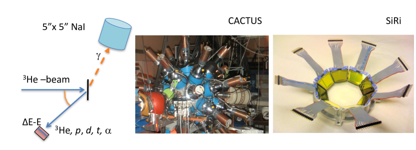
Figure 1: (Color online) Typical particle-$\gamma$ coincidence set-up for the Oslo method. The 64 silicon particle telescopes of SiRi are placed in the vacuum chamber at the center of CACTUS.

Figure 1 shows a schematic drawing of the set-up. A silicon particle detection system (SiRi) siri , which consists of 64 telescopes, is used for the selection of a certain ejectile types and to determine their energies. The front $\Delta E$ and back $E$ detectors have thicknesses of 130 $\mu$m and 1550 $\mu$m, respectively. Coincidences with $\gamma$ rays are performed with the CACTUS array CACTUS , consisting of 26 collimated $5"\times 5"$ NaI(Tl) detectors with a total efficiency of $14.1$% at $E_{\gamma}=1.33$ MeV.

With the raw $\gamma$-ray spectra at hand, we arrange these into a particle-$\gamma$ matrix $R(E,E_{\gamma})$. Then, for all initial excitation energies $E$, the $\gamma$ spectra are unfolded with the NaI response functions giving the matrix $U(E,E_{\gamma})$ gutt1996 . The procedure is iterative and stops when the folding ${\cal F}$ of the unfolded matrix equals the raw matrix within the statistical fluctuations, i.e. when ${\cal F}(U)\approx R$.

In the next step the primary $\gamma$-ray spectra are extracted from the unfolded matrix $U$. This is obtained by subtracting a weighted sum of $U(E^{\prime},E_{\gamma})$ spectra below excitation energy $E$:

$$P(E,E_{\gamma})=U(E,E_{\gamma})-\sum_{E^{\prime}<E}w(E,E^{\prime})U(E^{\prime},E_{\gamma}).$$ (1)

The weighting coefficients $w(E,E^{\prime})$ are determined in an iterative way described in Ref. Gut87 . After a few iterations, $w(E,E^{\prime})$ converges to $P(E,E_{\gamma})$, where we have normalized each $\gamma$ spectrum by $\sum_{E_{\gamma}}P(E,E_{\gamma})=1$. This conversion of $w\rightarrow P$ is exactly what is expected, namely that the weighting function should equal the primary $\gamma$-ray spectrum. We rely on the fact that quasi-continuum decay is dominated by dipole transitions kopecky1990 ; larsen2013 , and consider only $E1$ and $M1$ transitions in the following. It should be noted that the validity of the procedure rests on the assumption that the $\gamma$-energy distribution is the same whether the levels were populated directly by the nuclear reaction or by $\gamma$ decay from higher-lying states.

To extract the level density and the $\gamma$-ray strength function, we exploit a part of the primary $P(E,E_{\gamma})$ matrix where the level density is high, typically well above 2$\Delta$ (the pairing gap), and where no single $\gamma$ lines dominate. This statistical part of the matrix is described by the product of two vectors:

$$P(E,E_{\gamma})\propto\rho(E-E_{\gamma}){\cal{T}}(E_{\gamma}),\$$ (2)

where the decay probability is assumed to be proportional to the NLD at the final energy $\rho(E-E_{\gamma})$ according to Fermi’s golden rule dirac ; fermi . The decay is also proportional to the $\gamma$-ray transmission coefficient ${\cal{T}}$, which according to a generalized version of the Brink hypothesis brink is independent of spin and excitation energy; only the transitional energy $E_{\gamma}$ plays a role. The $\gamma$SF can be calculated from our measured transmission coefficient through kopecky1990

$$f_{XL}(E_{\gamma})=\frac{1}{2\pi}\frac{{\cal{T}}_{XL}(E_{\gamma})}{E_{\gamma}^{2L+1}}.$$ (3)

It remains to normalize $\rho$ and ${\cal{T}}$ to known experimental information from other experiments. The normalization procedures and the precisions obtained depend on available external data. Further description and tests of the Oslo method and the normalization procedures are given in Refs. Schiller00 ; Lars11 .

One could argue that the level densities and $\gamma$SFs would depend on the light-ion reaction used. However, although these reactions are very selective, the $\gamma$ decay appears much later and thus from a thermalized, compound-like system. This has been demonstrated by the Oslo group for many reactions. As an example, the $(^{3}$He, $\alpha\gamma)$ and $(^{3}$He, ³He’$\gamma)$ reactions have been studied populating the same final nuclei, ⁹⁶Mo and ⁹⁷Mo guttormsen2005 ; chankova2006 . Also the very different reactions $(p,p^{\prime}\gamma)$ and $(^{3}$He, $\alpha\gamma)$ into ⁵⁶Fe confirm the independence of the reaction larsen2013 . Minor differences may appear which probably are due to deviations in the spin distributions populated by the various reactions.

3 The evaluation of $\gamma$ width and lifetime

The $\gamma$ width ($\Gamma$) and lifetime ($\tau$) can be evaluated from the measured NLD and $\gamma$SF obtained with the Oslo method. However, one should note some differences when comparing with neutron capture data. First of all, significantly more levels are populated in the charged-particle reaction, giving a large spin distribution of typically $J\approx 0-6$ and populations of both parities. Secondly, the initial excitation bin is much larger (100-200 keV) than for neutron capture data that may even select only one ore a few resonances. These conditions ensures that the Oslo type of data represent an averaging over a broader initial excitation energy region and spins and parities.

The $\gamma$-decay strength function for $\gamma$-ray emission of multipole $XL$ from levels of spin $J$ and parity $\pi$ at $E_{x}$ is defined by Bartholomew et al. bart1973 as

$$f_{XL}^{J\pi}(E_{\gamma},E_{x})=\frac{\langle\Gamma_{XL}^{E_{\gamma}}(E_{x},J,\pi)\rangle\rho(E_{x},J,\pi)}{E_{\gamma}^{2L+1}},$$ (4)

where $\langle\Gamma_{XL}^{E_{\gamma}}(E_{x},J,\pi)\rangle$ is the partial $\gamma$ width for the transition $E_{x}\rightarrow E_{x}-E_{\gamma}$. In the equation, it is assumed that $E_{x}$ takes a fixed value while $E_{\gamma}$ takes variable values, i.e. the final excitation energy $E_{x}-E_{\gamma}$ varies. We now apply Eq. (3) with the assumption that $f_{XL}(E_{\gamma},E_{x})$ is independent of $E_{x}$ brink and find

$$\langle\Gamma_{XL}^{E_{\gamma}}(E_{x},J,\pi)\rangle=\frac{1}{2\pi\rho(E_{x},J,\pi)}{\cal T}_{XL}(E_{\gamma}).$$ (5)

In order to obtain the the average total $\gamma$ width of levels with excitation energy $E_{x}$, spin $J$ and parity $\pi$, we sum up the strength for all possible primary transitions below $E_{x}$ as prescribed by Kopecky and Uhl kopecky1990 :

$$\langle\Gamma(E_{x},J,\pi)\rangle=\frac{1}{2\pi\rho(E_{x},J,\pi)}\sum_{J_{f},\pi_{f}}\int_{0}^{E_{x}}{\mathrm{d}}E_{\gamma}{\cal T}_{XL}(E_{\gamma})\times\rho(E_{x}-E_{\gamma},J_{f},{\pi}_{f}),$$ (6)

where the summation run over all final levels with spin $J_{f}$ and parity $\pi_{f}$ that are accessible by $XL$ transitions with energy $E_{\gamma}$. It should be noted that for the normalization of ${\cal T}$, we apply Eq. (6) using the initial spin(s) populated in neutron capture to reproduce the total $\gamma$ width $\langle\Gamma(S_{n})\rangle$. If we for simplicity assume that all levels within the initial energy bin are populated in the charged particle reaction, we obtain the average total $\gamma$ width by

$$\langle\Gamma(E_{x})\rangle=\sum_{J\pi}g(E_{x},J){\cal P}(E_{x},\pi)\langle\Gamma(E_{x},J,\pi)\rangle,$$ (7)

where $g$ and ${\cal P}$ are the spin and parity distributions, respectively. From $\langle\Gamma(E_{x})\rangle$, we get the lifetime in the quasi-continuum by

$$\langle\tau(E_{x})\rangle=\frac{\hbar}{\langle\Gamma(E_{x})\rangle}=\frac{658.2\ }{\langle\Gamma(E_{x})\rangle}{\rm fs},$$ (8)

where the $\gamma$ width is in units of meV.

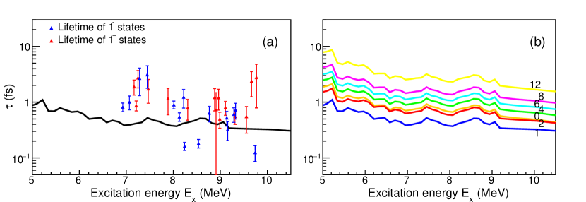
Figure 2: (Color online) Experimental lifetimes of $J^{\pi}=1^{+}$ and $1^{-}$ states in ⁵⁶Fe bauwens2000 ; shizuma2013 compared with the estimates from the Oslo method (black line) (a). The predictions for various spins are shown in panel (b).

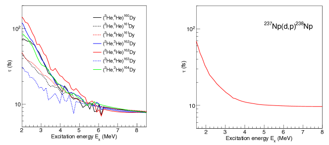
Figure 3: (Color online) Lifetimes in the quasi-continuum region for ^160-164Dy (a) and ²³⁸Np (b).

4 Results and discussion

The $\gamma$ widths and lifetimes of $J^{\pi}=1^{+}$ and $1^{-}$ states in the quasi-continuum of ⁵⁶Fe have been measured by photon-scattering experiments bauwens2000 ; shizuma2013 . In Fig. 2 (a) we show the measured lifetimes, and compare with the corresponding estimates of lifetimes evaluated from the NLD and $\gamma$SF obtained from the Oslo method larsen2013 . We observe that the experimental data fluctuate up to a factor of ten, which is a result of the random structural overlap with few final states. Assuming Porter-Thomas fluctuations PT , the relative fluctuations are $\sqrt{2/\nu}$ where the degree of freedom $\nu$ can be estimated by the number of primary transitions from the excited state. Figure 2 (b) shows that the spin 1 states represent the fastest dipole transitions in the quasi-continuum, which can be explained by their direct decay to the $0^{+}$ ground and first excited $2^{+}$ states.

The number of levels in odd-mass dysprosiums are about a factor of seven larger than for the even-even neighbours. This reduces the decay time for the odd-mass isotopes as seen in Fig. 3 (a). However, at higher excitations $(E_{x}\geq 5$ MeV) the lifetimes for all isotopes converge to a common value. Furthermore, Fig. 3 (b) demonstrates that the lifetimes of ²³⁸Np seem to flatten out for $E_{x}\geq 4$ MeV. The saturation in $\tau$ seen for the two cases can be understood from Eq. (6): the decay by higher $\gamma$ energies for higher $E_{x}$ is suppressed by a factor $\exp{(-E_{\gamma}/T)}$ where $T$ is the nuclear temperature. It is surprising that the saturation in lifetimes is the same ($8-10$ fs) for a large range of mass numbers.

References

- (1) A. Schiller et al., Nucl. Instrum. Methods Phys. Res. A 447 494 (2000).
- (2) M. Guttormsen et al., Nucl. Instrum. Methods Phys. Res. A 648, 168 (2011).
- (3) M. Guttormsen et al., Phys. Scr. T 32, 54 (1990).
- (4) M. Guttormsen et al., Nucl. Instrum. Methods Phys. Res. A 374, 371 (1996).
- (5) M. Guttormsen et al., Nucl. Instrum. Methods Phys. Res. A 255, 518 (1987).
- (6) P. A. M. Dirac, Proc. R. Soc. Lond. A 1927 114, 243-265.
- (7) E. Fermi, Nuclear Physics. University of Chicago Press (1950).
- (8) D. M. Brink, Doctoral thesis (unpublished), Oxford University, 1955.
- (9) J. Kopecky and M. Uhl, Phys. Rev. C 41, 1941 (1990).
- (10) A. C. Larsen et al., Phys. Rev. C 83, 034315 (2011).
- (11) M. Guttormsen et al., Phys. Rev. C 71, 044307 (2005).
- (12) R. Chankova et al., Phys. Rev. C 73, 034311 (2006).
- (13) A. C. Larsen et al., Phys. Rev. Lett. 111, 242504 (2013).
- (14) G. A. Bartholomew et al., Adv. Nucl. Phys. 7, 229 (1973).
- (15) F. Bauwens et al., Phys. Rev. C 62, 024302 (2000).
- (16) T. Shizuma et al., Phys. Rev. C 87, 024301 (2013).
- (17) T. Porter and R. G. Thomas, Phys. Rev. 104, 483 (1956).