GRB: Greedy Routing Protocol with Backtracking for Mobile Ad Hoc Networks
(Extended Version)

Abstract

Routing protocols for Mobile Ad Hoc Networks (MANETs) have been extensively studied for more than fifteen years. Position-based routing protocols route packets towards the destination using greedy forwarding (i.e., an intermediate node forwards packets to a neighbor that is closer to the destination than itself). Different position-based protocols use different strategies to pick the neighbor to forward the packet. If a node has no neighbor that is closer to the destination than itself, greedy forwarding fails. In this case, we say there is void (no neighboring nodes) in the direction of the destination. Different position-based routing protocols use different methods for dealing with voids. In this paper, we use a simple backtracking technique to deal with voids and design a position-based routing protocol called “Greedy Routing Protocol with Backtracking (GRB)”. We compare the performance of our protocol with the well known Greedy Perimeter Stateless Routing (GPSR) routing and the Ad-Hoc On-demand Distance Vector (AODV) routing protocol as well as the Dynamic Source Routing (DSR) protocol. Our protocol needs much less routing-control packets than those needed by DSR, AODV, and GPSR. Simulation results also show that our protocol has a higher packet-delivery ratio, lower end-to-end delay, and less hop count on average than AODV.

Keywords: MANETs, Routing in MANETs, Geographic routing.

1 Introduction

A Mobile Ad-hoc Network (MANET) consists of a set of nodes each of which is capable of being both a host and a router. The nodes form a network among themselves without the use of any fixed infrastructure, and communicate with each other by cooperatively forwarding packets on behalf of others. Mobile ad-hoc networks have applications in areas such as military, disaster rescue operations, monitoring animal habitats, etc. where establishing communication infrastructure is not feasible [1, 2, 3, 4, 5]. Routing protocols designed for mobile ad hoc networks need to be scalable, robust, and have low routing overhead. Routing protocols designed for MANETs can be broadly classified as geographic routing protocols (or position-based routing protocols) and topology-based routing protocols. In geographic routing protocols, nodes do not maintain information related to network topology (i.e., they are topology independent). They only depend on the location information of nodes to make forwarding decisions. Generally [6], nodes need their own location, their neighbors’ location, and the location of the destination node to which the packet needs to be forwarded. Using this location information, routing is accomplished by forwarding packets hop-by-hop until the destination node is reached [7]. Greedy forwarding (GPSR [8]), is one of the main strategies used in geographic routing protocols. Under Greedy forwarding, an intermediate node on the route forwards packets to the next neighbor node that is closer to the destination than itself.

Topology-based routing protocols depend on current topology of the network. Topology-based routing is also known as table-based routing. Topology-based routing can be classified in to proactive routing protocols, reactive routing (on-demand) protocols, and hybrid routing protocols [1, 9, 10]. In proactive protocols, like DSDV [11], nodes use pre-established table-based routes [12]. Therefore, routes are deemed reliable and nodes do not wait for route discovery which cuts off latency. However, overhead incurred for route construction and maintenance can degrade performance, limit scalability, and the routing table will consume lot of memory as the network size grows.

Reactive Routing Protocols are also called on-demand routing protocols wherein senders find and maintain route to a destination only when they need it. Reactive routing needs less memory and storage capacity than proactive protocols. However, in network areas where nodes can move more unpredictably and frequently, path discovery may fail since the path can be long and links may break due to node mobility or when facing other obstacles [1]. The delay caused by route discovery for each data traffic can increase latency.

On the other hand, geographic routing protocols require only the location information of nodes for routing. They do not require a node to establish a route to the destination before transmitting packets. Unlike on-demand routing protocols, they do not depend on flooding route request messages to discover routes. This feature helps geographic routing protocols to reduce the extra overhead imposed by topology constraints for route discovery [13, 7]. A node only needs to know the position of its neighbors and the position of the destination to forward packets. Therefore, geographic routing protocols generally are more scalable than topology based routing protocols [14, 15, 16]. In spite of the benefits mentioned above, geographic routing protocols have the following limitations: Greedy forwarding, the primary packet forwarding strategy used by geographic routing protocols, may fail in low density networks, networks with non-uniformly distributed nodes, and/or networks where obstacles can be present. Moreover, Location Service is required to obtain location information of destination nodes which may result in high overhead. The non-hierarchical address structure used in ad-hoc networks requires more control overhead to update node location [14].

Paper Objective

Many geographic routing protocols construct the planarized version of the local network graph to route a packet around voids; constructing planarized graph of the local network requires exchanging neighborhood information of nodes at least two hops away and then planarizing the graph, which can cause large overhead, especially in a sparse network wherein several voids may exist on a route. In addition to that, planarization may fail to generate bidirectional, connected, and/or cross link free local graphs as observed by Kim et al. and Frey et al. [17, 18]. In this paper, we address this issue and propose a simple geographic routing protocol that uses backtracking to route packets around voids.

Organization of the Paper

The rest of the paper is organized as follows. In Sect. 2, we discuss the related work and paper objectives. In Sect. 3, we present our protocol. In Sect. 4, we present the performance evaluation results of our protocol. In Sect. 5 we give a brief discussion of our protocol. Sect. 6 concludes the paper.

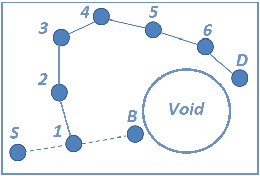
Figure 1: Example Illustrating Dead End (void) in Greedy Forwarding.

2 Related Work

In this section, we discuss the basic idea behind several of the recently proposed geographic (position-based) routing protocols and on demand routing protocols bringing out their week and strong points.

2.1 Position-based Routing Protocols

GPSR [8], a well known geographic routing protocol proposed by Karp and Kung, uses greedy forwarding as the default forwarding strategy. When a packet confronts a void (i.e., when greedy forwarding fails), they planarize the local topology graph either by constructing the Relative Neighborhood Graph (RNG) or Gabriel Graph (GG) of the local network graph and use those graphs to route around the void. However, constructing such graphs involves overhead.

Zhao et al. [13], proposed a routing protocol called HIR. HIR selects specific nodes as landmarks and builds a multidimensional coordinate system based on which they find the Hop ID distance between each pair of nodes in the network. When a packet meets with a void, the protocol switches to a landmark-guided, detour routing which tries to forward the packet to the landmark nearest to the destination. This protocol does not scale well due to the central packet flooding technique used by a designated node to select LANDMARKs. Nodes proportionally exchange high amount of control information to select LANDMARKs. However, since this happens only to select LANDMARKs, normal data packet forwarding process does not produce additional overhead. On the other hand, the level of stability of LANDMARK nodes plays a significant role in control overhead.

Li and Singhal [1] proposed ARPC in which the routing process is divided into several parts. First, Location-based Clustering Protocol in which several physical locations are assumed to be known in the network area which are called anchors and they have coordinates. Second, Inter-cell Routing Protocol which lets every node maintain a dynamic routing table that contains routes to its neighboring cells. Third, Intra-cell Routing Protocol which is an on-demand routing technique that is performed inside the same cell. Fourth, Data Packet Routing which deals with how the data packets are routed from a source to a destination node. ARPC is less scalable since nodes use routing tables which can become large as the network size increases. Moreover, the announcement packets sent by agent nodes to announce their existence to the nodes in the cell they reside can cause large overhead as the node density increases.

Lin and Kus proposed LGR [6] which is a location-fault-tolerant geographic routing protocol that uses both traditional geographic routing and position-based clustering technique. Routing is performed using global geographic routing and local gradient routing. A cluster head (CH) broadcasts messages to all the nodes in its own cluster as well as all nodes in its neighboring clusters so that each of these nodes can establish a routing path to the CH. This process affects scalability. If nodes are highly mobile, frequent CH election occurs which results in more message broadcasting by newly elected CHs to announce their existence which overwhelms nodes with control packets exchanged between nodes and hence limits scalability.

Zhou et al. presented Geo-DFR [19] which incorporates directional forwarding in routing (DFR) [20]. Routing is done mainly using greedy forwarding. However, in case of dead ends (voids), DFR is used. Geo-DFR improves DFR to solve the dead end problem and avoids face routing. The authors use Fisheye State Routing protocol (FSR) [21] which is the protocol that is ”hosting” Geo-DFR. Scalability of Geo-DFR is affected by different factors. First, maintaining three tables in each node increases overheard especially when a node has many neighbors. But this limitation is local, since the number of records in two of these tables depends on the density of the neighboring nodes.

Li et al. [22] proposed localized load-aware geographic routing using the concept of cost-to-progress ratio in greedy routing (CPR-Routing). The main idea behind this protocol is to combine the greedy forwarding technique and localized cost-to-progress ratio (CPR) [23]. The load awareness used in this protocol tends to minimize load and maximize progress geographically towards the destination; however, this is difficult to achieve, so it tries to balance the two factors in making routing decisions. A drawback of this approach is the complexity involved in the calculation for selecting appropriate neighbor to forward a packet which could result in higher end-to-end delay.

Macintosh et al. proposed LANDY [24] which uses locomotion (movement) and velocity of each node to predict the future location of each of these nodes so that data packets are forwarded efficiently towards the destination nodes. LANDY uses only local broadcasting to build a Locomotion Table (LT). When forwarding fails, instead of broadcasting, a recovery mode is invoked from the point of failure, allowing the protocol scale better. Overhead involved in this protocol is higher than that of the protocols discussed so far since it uses more control information to build tables at each node. That includes different samples of each node’s location information exchanged periodically between nodes and building planar graphs to be used as alternatives to the normal forwarding mode.

2.2 On-demand Routing Protocols

We compare our protocol with two of the well-known on-demand routing protocols that are discussed bellow. Under AODV [25], when a node needs to establish a route to a destination, it broadcasts a route request to all its neighbor nodes. A node receiving the route request node replies to the source node, if it has a route to the destination; otherwise, it rebroadcasts the route request to all its neighbors. This process continues until the a route to the destination is found. This protocol is robust because broadcasting route request guarantees finding a route to the destination if there is one; however, as number of nodes increase, the number of redundant rebroadcasting of route requests increases. This means this protocol is not scalable.

Under DSR [26], when a node $S$ needs to find a route to a node D, it broadcasts a Route Request packet (RREQ). On receiving RREQ, an intermediate node adds its id to the list of nodes in RREQ if it has no route to the destination $D$ and if its id is not in already in the list; then it rebroadcasts the updated RREQ packet. When a target node receives the RREQ, it puts the list of nodes received in RREQ in the Route Reply (RREP) and sends it back to the sender S. When $S$ receives the RREP, the sender caches the route for subsequent routing. This protocol also results in redundant propagation of route requests.

3 Problem Statement and Design of our Protocol

In this section, we first present the objective of the paper and the basic idea behind our protocol, and then present a detailed description of the protocol.

3.1 Problems Addressed and Solved in This Paper

Greedy forwarding, the primary packet forwarding strategy used by geographic routing protocols, may fail in low density networks, networks with non-uniformly distributed nodes, and/or networks where obstacles can be present. Therefore, the main problem with greedy forwarding strategy is that it does not guarantee packet delivery to the destination because of the dead end phenomenon even if there is a route to the destination. Figure 1 shows an example of dead end (void) problem. When the source node $S$ needs to send packets to the destination node $D$, it forwards the packets greedily to a node that is closer to the destination than itself. On receiving the packets, each subsequent node does the same. When the packets reach node $B$, it finds that none of its neighbors are closer to the destination node $D$ than itself and $D$ is outside the transmission range of node $B$. This means there is a void between $B$ and $D$ as depicted in Figure 1. Even though there is a valid path from $S$ to $D$ through intermediate nodes 1,2,3,4,5, and 6, greedy forwarding cannot use it. This means, under pure greedy forwarding, packets may be dropped even though there are valid paths to destination nodes.

Generally, position-based routing protocols use planarization and face routing [8, 14] to go around voids. Planarization involves constructing the planar graph of local network. Graphs are generally planarized using the Gabreil Graph (GG) [27] or the Relative Neighborhood Graph (RNG) [28]. However, planarization may fail to generate bidirectional, connected, and/or cross link free local graphs as observed by Kim et al. and Frey et al. [17, 18]. This may be the result of node’s incorrect estimate of its location or irregular communication range as a result of radio-opaque obstacles or transceiver differences.

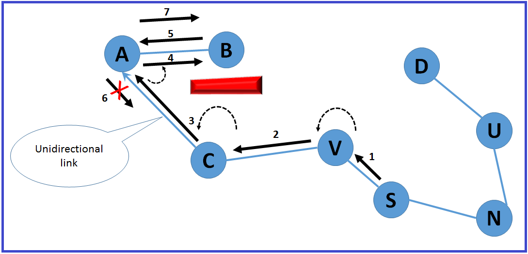
Figure 2: Example of Planarization where a Unidirectional Link Causes Routing Failure.

As shown in Figure 2, a unidirectional link can cause an infinite loop during face traversal. In this example, when the source node $S$ needs to send data packets to the destination node $D$, based on greedy forwarding, it sends that data packet to node $V$. Node $V$ is a dead end for that packet, hence it switches to face routing and forwards the data packets to node $C$. In this case, when $C$ constructs the planar graph of the local network using $GG$, it cannot see the witness $B$ in the circle whose diameter is the distance between $A$ and $C$ because of the obstacle shown in Figure 2. Therefore, $C$ generates a link to node $A$. However, node $A$ does not create a link to node $C$ in its local graph because it can see the witness $B$ in the circle. Therefore, node $C$ can forward the data packets to node $A$ which in turn forwards them to node $B$ and based on face routing, node $B$ returns the packet to node $A$. Since node $A$ does not have a link to node $C$ in the local graph, it returns the packets to node $B$ and as a result, the data packets loop.

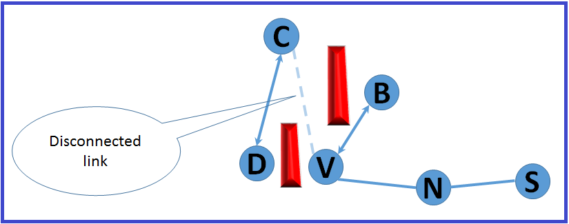
Figure 3: Example of Planarization where a Disconnected Link Causes Routing Failure.

Routing can also fail because of disconnected links as shown in Figure 3. In this example, source $S$ needs to send data packets to destination $D$. When packets arrive at node $V$, they face a dead end and switch to face routing. From node $V$’s view, $B$ is a witness and from $C$’s view, $D$ is a witness. Therefore the link between $V$ and $C$ is removed in the planarized graph of local network and as a result, the local graph is disconnected and packets cannot travel to $D$.

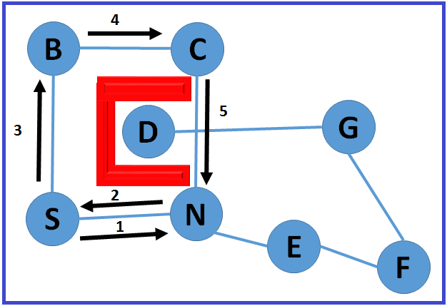
Figure 4: Example of Planarization where a Cross Link Causes Routing Failure.

Another scenario wherein routing may fail is shown in Figure 4. In this example, when node $S$ needs to send data packets to destination $D$, it first forwards the packet to next closer neighbor $N$ which faces void and hence, creates a local planner graph. The obstacle shown in Figure 4 hides $D$ from both $N$ and $C$ and as a result, a link between these two nodes is created which crosses the link between $D$ and $G$. Then, based on face routing and right hand rule, $N$ returns the packet back to $S$ which in turn forwards it to $B$. From $B$, the packet is forwarded to $C$ and then to $N$ where it loops.

This means that face routing cannot always forward packets when they face void even when alternative valid paths exist. We address this problem and present an algorithm which uses a simple backtracking technique to route around voids as explained below.

When pure greedy forwarding is used, packets are dropped when they face voids making recovery procedures necessary. The existing protocols mainly depend on face routing (e.g.,GPSR) [8] to recover from voids. However, in addition to failing to go around voids in some scenarios as explained above, face routing can incur high processing cost and high end-to-end delay.

We address these issues and propose Greedy Routing Protocol with Backtracking for MANETs (GRB). GRB is a novel and simple position based routing protocol which allows each node to forward data packets to its best neighbor possible until the destination is reached. Unlike GPSR, GRB uses less computation to determine the next hop on the route.

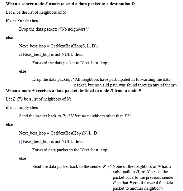
Figure 5: GRB data forwarding (Sending/Receiving Data Packets).

Figure 6: GRB data forwarding (Functions).

3.2 Basic Idea Behind Our GRB Protocol

GRB routes data packets either in forwarding mode (greedy mode or simple forwarding) or in backtracking mode. When a sender/intermediate node $S$ wants to send/forward a packet to a destination $D$, it picks its $best$ $neighbor$ $N1$ and sends the packet to $N1$. The best neighbor $N1$ is determined as follows: It picks the neighbor that is closest to the destination than any other neighbor; note that this neighbor may not be closer to the destination than $S$ itself because $S$ may be facing a void. If the packet backtracks from this node to $S$, it picks the one that is closest to the destination among the remaining neighbors, and this process continues until all neighbors have been tried; if it cannot forward the packet through any of its neighbors, it sends the packet back to the node from which it received the packet. Every node on the path uses the same strategy to forward packets. Note that if the node picked is closer to the destination than $S$, then the forwarding is implicitly greedy; otherwise, forwarding is around the void. In this protocol, a source node drops data packets if it has no neighbors, it tried all the neighbors to forward the packet and failed, or the number of times the packet backtracked reached a predetermined threshold.

Formal description of the protocol for data forwarding and finding the next best hop is given in Figures 5 and  6.

3.3 Assumptions

We assume that all nodes have the same transmission range (i.e., all links are bidirectional). We also assume that each node is equipped with a GPS and each node can get the location of the destination node through an available Location Service. In the following subsections we describe our protocol in detail.

3.4 Data Structures Used in the Protocol

Each node maintains the following two tables.

• Neighbor Table.

  Each node sends a $HELLO$ packet to all its neighbors in each time interval $T$. This $HELLO$ packet includes the node’s id as well as its position. To minimize collision of $HELLO$ packets due to concurrent transmissions, we jitter each $HELLO$ packet transmission interval by $R$ milliseconds between two successive transmissions of $HELLO$ packets so that each node transmits $HELLO$ packets at a random time chosen in the interval [$T-R$, $T+R$]. When a node receives a $HELLO$ packet, it creates in its Neighbor Table an entry containing neighbor identifier (NbrID), neighbor position, and lifetime if that neighbor is not in the table; the lifetime is updated if already there is an entry corresponding to that neighbor. If a node does not receive $HELLO$ packets for a time longer than $2T$ from a neighbor node, it assumes the neighbor has moved and removes the associated entry from the table.

• Seen Table.

  This table helps picking best neighbor for forwarding packets to the destination. For that purpose, when a node receives a data packet, it stores the information about the packet in its Seen Table. As shown in Table 1, each record of this table contains five fields namely, neighbor ID (NbrID), source address (Src), destination address (Dst), flag (Flag), and lifetime (Lifetime). $NbrID$ is the address of the neighboring node that has sent the packet, forwarded the packets, or the node from which the packet has backtracked. $Src$ contains the address of the source node that generated the data packet. $Flag$ indicates whether the received packet is a new packet (i.e., forwarding mode) or it has backtracked from a neighboring node (i.e., backtracking mode). The flag is set to $FALSE$ when the packet is in forwarding mode and set to $TRUE$ when it has backtracked. The lifetime field specifies the lifetime of the associated record in the Seen Table. When a node receives a data packet, it creates an entry in its Seen Table if the packet is new. However, if it has received a data packet with the same source and destination addresses from the same neighboring node, then it updates the lifetime of the associated record. On the other hand, when the lifetime expires, the associated record is removed from the table.

3.5 Sending and Forwarding Packets

Each node can send, forward, and/or receive data packets. When a node has data packets to send/forward and the destination node is not one of its neighbors, it picks the best neighbor using the method described in Sect. 3.2 and sends/forwards the packet to that neighbor. Since our protocol does not enforce the next-hop $N$ to be closer to the destination than the sender $S$, $N$ is either closer to $D$ than $S$ (i.e., Greedy mode), or farther to $D$ than $S$. However, the next-hop $N$ must be closer to $D$ than any other neighbor that has not seen a packet to the same source-destination pair according to their Seen Table. Before forwarding the packet to $N$, the source or intermediate node $S$ does the following:

Figure 7: Data forwarding Example.

• $S$ looks up its Seen Table for $N$.

  If $S$ has a record for $N$ with the same source and destination addresses as that in the packet, then it considers $N$ as invalid next hop for that packet and picks another neighboring node as the next hop. This means that $S$ has received this packet from $N$ which is either a new packet (i.e., flag is FALSE) or a backtrack packet (i.e., flag is TRUE). Therefore, it cannot forward the packet to that node because that results in a loop. For example, in Figure 7, if the node $N3$ receives a data packet from node $N1$, it creates an entry in its Seen Table as shown in Table 1. This entry tells $N3$ that $N1$ is invalid next hop because it has received the packet from $N1$ and as a result, the Seen Table prevents loop between $N3$ and $N1$. However, the Seen Table of $N1$ does not have $N3$ as a neighbor node so it can forward data packets to $N3$.

  Table 1: Seen Table at Node $N3$ in Figure 7

  NbrID	Src	Dst	Flag	Lifetime
  $N1$	$S$	$D$	False	$T$

• $S$ verifies with $N$ if it is a valid next hop.

  If $N$ is not in the Seen Table of $S$, then $S$ sends $N$ a verification packet, with same source-destination pair in the header as in the data packet’s header, asking $N$ to check whether it has seen data packets for the same source-destination pair from any of its other neighbors. When $N$ receives the verification packet, it checks its Seen Table for an entry that has the same source and destination addresses as that in the verification packet, with a Flag set to $False$, but with NbrID different from the ID of $S$. If such an entry is found, it means that $N$ has seen a packet for the same source-destination pair and it sends a reply back to $S$ indicating that it is invalid next hop. However, if such an entry is found but with Flag set to $True$, it means a neighbor $N1$ of node $N$ has sent back the data packet to $N$ after $N1$ failed to forward the packet. In this case, maybe there are neighbors of $N$ other than $N1$ that have not tried to forward the packet yet, therefore $N$ is not considered as invalid next hop and as a result, $N$ sends a reply back to $S$ indicating that it is a valid next hop for that data packet. After receiving the reply from $N$, if $S$ finds $N$ is a valid next hop, it forwards the packet to $N$. Otherwise, it picks another neighbor as a new candidate for next hop and checks if it is a valid next hop and so on. For example, in Figure 7, when $N1$ needs to send a data packet to $N3$, it sends a verification packet to $N3$. $N3$ checks its Seen Table for an entry with NbrID set to any ID other than $N1$, same Src and Dst values as those in the verification packet, and Flag set to $False$. However, $N3$ does not have such entry in its Seen Table (refer to Table 1), hence $N3$ sends a positive reply to $N1$, and $N1$ forwards the packet to $N3$. If a node finds all its neighbors are invalid next hops, then the packet is sent back to the node from which it was received.

• Packet backtracks.

  A packet backtracks from the current node to its sender in the following two cases:

  1. All the neighbors of the current (intermediate) node have seen that packet. This means none of the neighbors could forward the packet.

  2. The current node has no neighbors other than the sender. For example, in Figure 7, $N2$ has no neighbors other than $N1$ which sent the packet to it. Therefore, the packet backtracks to $N1$ and $N1$ inserts a new entry to its Seen Table as shown in Table 2. The Flag of the new entry (i.e., second row) is set to $True$ which means that from the perspective of $N1$, $N2$ is considered invalid next hop for that packet. Hence, when $N1$ tries to pick next hop for the same destination next time, it will not pick $N2$ as long as the Lifetime of the associated entry (i.e., second row in Table 2) in the Seen Table of $N1$ has not expired.

  Table 2: Seen Table at Node $N1$ in Figure 7

  NbrID	Src	Dst	Flag	Lifetime
  $S$	$S$	$D$	False	$T1$
  $N2$	$S$	$D$	True	$T2$

  Table 3: Topology used for Simulation

  Nodes	Network Area	CBR Flows	Packets Sent
  {50,75,100,125,150,175,200,225,250,300}	1500m X 1500m	30	8780
  50	1500m X 300m	30	8780
  112	2250m X 450m	30	8780
  200	3000m X 600m	30	8780

• Packet is dropped. A packet is dropped by a source node when all the neighbors have been identified as invalid next hops or the source node has no neighbors.

4 Performance Analysis

In this section, we present the performance evaluation results of GRB compared to AODV [25], DSR [26], and GPSR [8]. We first describe the simulation environment and then discuss the simulation results. We simulated GRB, AODV, and DSR on a variety of network topologies to compare the performance. We also compared the performance of GRB with that of GPSR using the results provided in GPSR [8].

4.1 Simulation Environment

We used GloMoSim [29], a network-simulation tool for studying the performance of routing protocols for ad-hoc networks, for evaluating the performance of GRB. We chose IEEE 802.11 and IP as the MAC and network layer protocols, respectively. All nodes have a fixed transmission range of 250 m. We used the implementation of AODV and DSR that comes with the GloMoSim 2.0.3 package to compare their performance with GRB. We ran several simulations on two different sets of traffic flows. The simulations run in different terrain areas are shown in Table 3; each simulation lasted for 900 seconds of simulated time. The nodes were distributed uniformly at random in the network area. We used the following four metrics to evaluate performance:

1. Packet Delivery Ratio: Measures the success rate of delivered data packets.

2. End-to-End Delay: Average time a packet takes to reach the destination node.

3. Hop Count: The number of hops a packet traverses to reach the destination.

4. Node Density: Number of nodes in the area.

5. Network Diameter: Studying the effect of different network areas.

In this experiment, we varied the number of nodes simulated from 50 to 300. Two sets of random traffic flows have been used in the simulation. The first set is 30 CBR (Constant Bit Rate) flows in which different senders generate data packets to be forwarded to destinations. Each CBR flow sends packets at speed of 2Kbps and uses 64-byte packets. Depending on the start time and end time of each sender in each flow, different number of packets are sent by different CBR flows. However, in each and every flow, each sender sends a packet every 0.25 second. Node mobility is set using random Way-point [26] model. Under this model, each node travels from a location to a random destination at a random speed, the speed being uniformly distributed in a predefined range. After a node reaches its destination, it pauses for a predetermined amount of time and then moves to a new destination at a different randomly chosen speed. In our simulation, the speed randomly chosen lies between 0 and 20 meters/second. In order to study how mobility affects the performance of the routing protocols, we selected pause times of 0, 20, 30, 40, 60, 80, 100, and 120 seconds. When the pause time is 0 seconds, every node moves continuously. As the pause time increases, the network approaches the characteristics of a fixed network. The second set consists of 20 CBR flows which has 20 sender nodes generating packets at a speed and size same as that in the first set.

4.2 Packet Delivery Ratio

The overall average packet delivery ratio for DSR, AODV, and GRB are 55.52%, 97.38% and 98.60%, respectively. We select CBR flows randomly, hence it is not known whether there is a valid path between the source node and the destination node in each flow. Higher number of packets (refer to Table 3) imposes higher demand on routing protocols as higher traffic is generated between source and destination pairs. GRB finds next hops locally with the most up to date location information of the nodes involved in the forwarding process. It simply picks next hops based on Seen Tables to forward data packets which results in few control packets. This makes GRB adapt locally to location changes, hence it tolerates mobility better than AODV and DSR. Therefore, GRB delivers higher number of data packets than DSR and AODV for different pause times as shown in Figures 9, 9, 11, and 11.

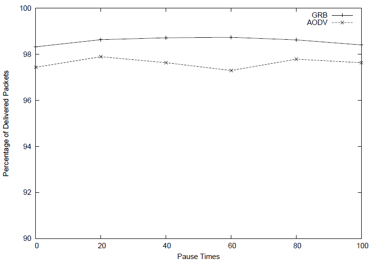
Figure 8: Packet Delivery Ratio (50 Nodes, 30-CBR Flows, network area (1500m x 300m)), GRB compared with AODV.

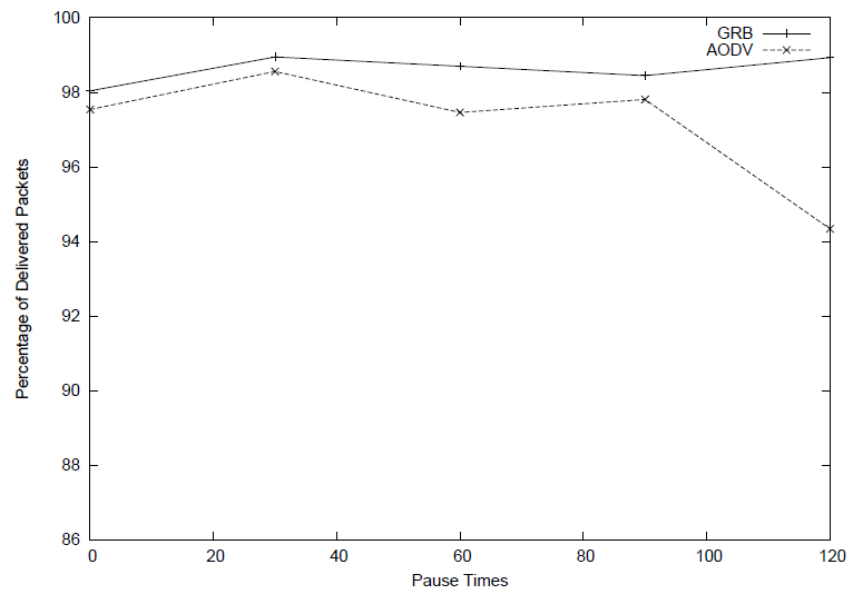
Figure 9: Packet Delivery Ratio (50 Nodes, 20-CBR Flows, network area (1500m x 300m)), GRB compared with AODV.

Figure 10: Packet Delivery Ratio (50 Nodes, 30-CBR Flows, network area (1500m x 300m)), GRB compared with DSR.

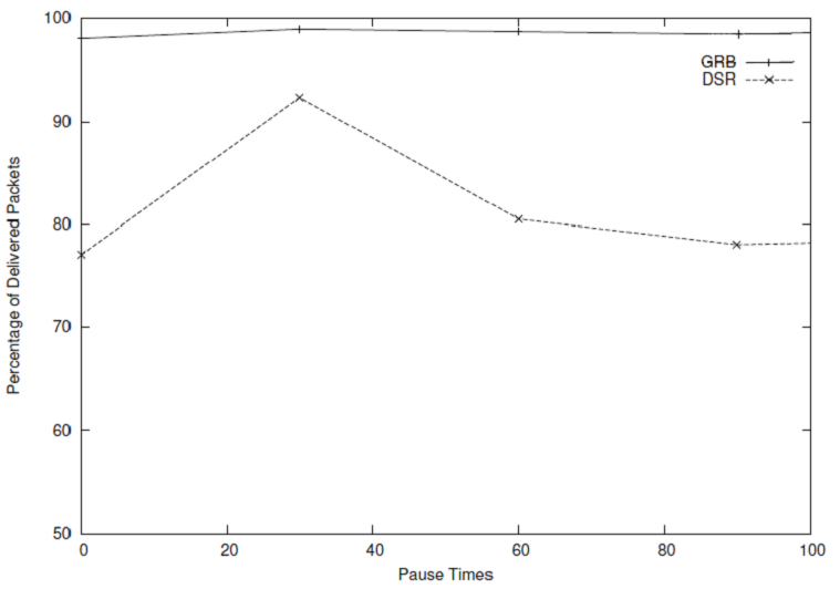
Figure 11: Packet Delivery Ratio (50 Nodes, 20-CBR Flows, network area (1500m x 300m)), GRB compared with DSR.

Figure 12: Average End-To-End Delay (50 Nodes, 30-CBR Flows, network area (1500m x 300m)), GRB compared with AODV.

Figure 13: Average End-To-End Delay (50 Nodes, 20-CBR Flows, network area (1500m x 300m)), GRB compared with AODV.

4.3 End-to-End Delay

As shown in Figures 13 and 13, the overall average end-to-end delay for AODV and GRB are 22.17 milliseconds and 14.98 milliseconds, respectively. For each CBR flow, we take the average end-to-end delay of all the packets received by the destination node in that flow. Then, we take the average delay of all the CBR flows. Because of its simplicity, GRB takes less time to deliver data packets in most of the scenarios. As shown in Figures 13 and 13, packets take more than 18 milliseconds on average to reach their destinations under AODV; however GRB delivers packets in less than 16 milliseconds. We can see GRB delivers packets much faster when network size and area is moderately small (50 nodes, (1500m x 300m) area). That is because most of the packets find greedy paths which take less calculation time and the decision is taken quickly based on the neighbors’ location information and their status regarding whether or not they are valid next hops. However, under AODV, data packets should wait for the route to be set up. Moreover, routes discovered under AODV may not be shorter than those discovered under GRB, because GRB uses greedy approach. As a result, AODV results in higher average end-to-end delay.

4.4 Node Density

Since our protocol uses only information about neighbors in forwarding decision, as node density increases, GRB keeps delivering higher fraction of data packets than AODV and DSR as shown in Figures 15 and 15. That is because both AODV and DSR depend on end-to-end route to forward data packets and that route is affected by mobility of the nodes and the size of the network. Hence due to mobility, more frequent link breaks occur leading to more route repair and setup and as a result, packets are lost more frequently. However, since the average end-to-end delay is taken only for packets that are delivered to their destinations and because data packets follow existing routes which decreases waiting time, AODV routes data packets in slightly less time than GRB when number of nodes grows to more than 200 as shown in Figure 17. However, GRB is faster in smaller networks (less density) because less computation required by nodes to make forwarding decisions since nodes have less neighbors. Average hop count is another parameter that we measure in this simulation to show that our protocol routes data packets with less number of hops as node density increases. For this metric, only the successfully delivered data packets are counted in the simulation results for both GRB and AODV. As shown in Figure 17, in smaller networks (i.e., less than 150 nodes), AODV uses less number of hops to forward data packets than GRB because there are more voids in sparse networks. This makes GRB data packets to go around voids through either next best hop or backtracking technique which makes GRB packets traverse more hops than AODV. However, as number of nodes increases, number of voids decreases and data packets move through greedy paths, hence GRB uses less number of hops than AODV in dense networks. It is worth to mentioning that under GRB, average hop count is also reduced because next hop is chosen greedily.

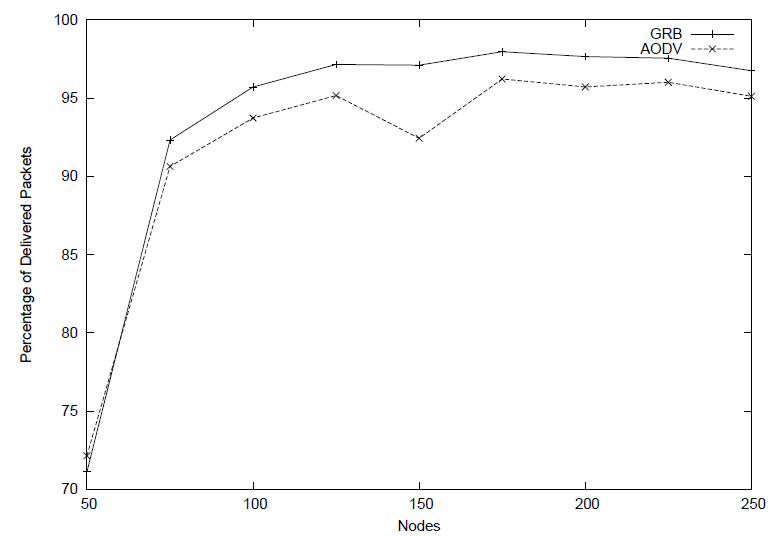
Figure 14: Packet Delivery Ratio as Number of Nodes increases (Network Area (1500x1500)), GRB compared with AODV.

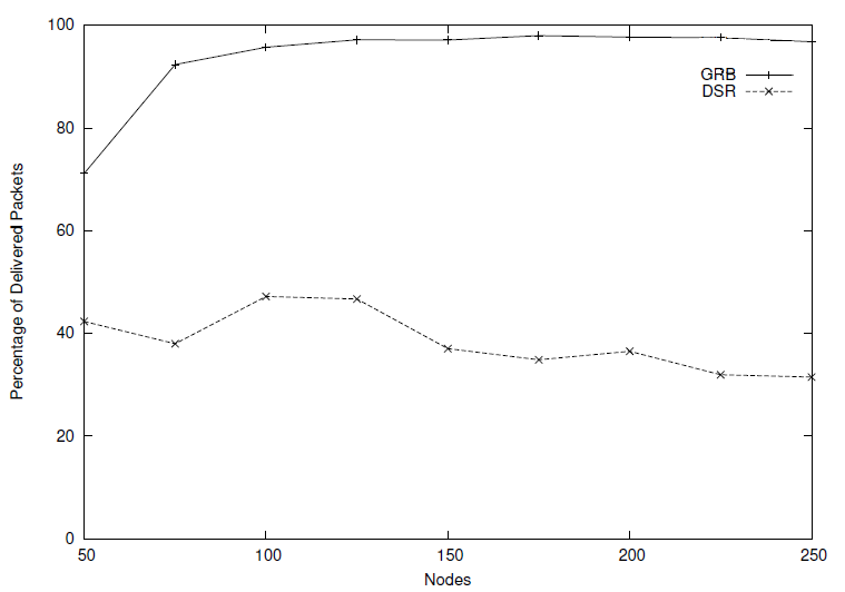
Figure 15: Packet Delivery Ratio as Number of Nodes increases (Network Area (1500x1500)), GRB compared with DSR.

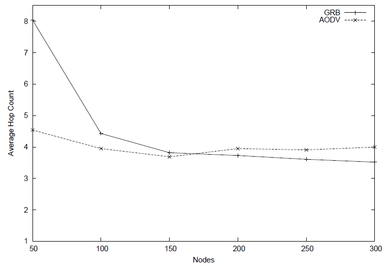
Figure 16: Average Hop Count as Number of Nodes increases (Network Area (1500x1500)), GRB compared with AODV.

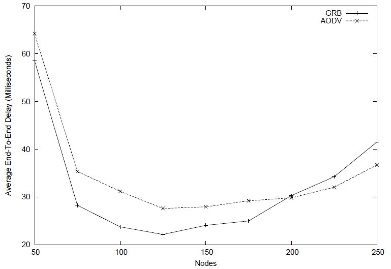
Figure 17: Average End-To-End as Number of Nodes increases (Network Area (1500x1500)), GRB compared with AODV.

4.4.1 Network Diameter

Figures 19 and 19 present packet delivery ratio results and Figures 23 and 23 present average hop count results for 112-nodes and 200-nodes networks with same CBR traffic and same node density for both networks. In these simulations, the terrain area within which nodes move are (2250x450) meters and (3000x600) meters respectively. In these simulations, we evaluate the effect of changing network diameter on success rate and hop count for both GRB and AODV. The probability of a route breaking increases as the route grows longer. GRB’s packet delivery ratio is higher than AODV and DSR under all pause times on larger networks; this is because GRB incurs no penalty when the length of the route increases since GRB uses only local topology information to find the next best hop. Moreover, GRB recovers from loss of neighbor (next hop) instantaneously by simply finding another candidate next hop which will take over the forwarding process. However, AODV’s percent delivery ratio decreases considerably as the network diameter increases because it needs to maintain longer end-to-end routes. DSR incurs higher traffic overhead in wider networks since it needs to maintain longer end-to-end source routes, hence its success rate decreases accordingly and it is much lower than that of GRB as shown in Figures 21 and 21. For the hop count metric, we calculate the average of all the received packets by all the destination nodes under all the flows for both GRB and AODV routing protocols. In small areas, AODV traverses less paths in higher mobility rates (i.e., lower pause times); however, GRB uses less hop counts when node mobility decreases (i.e., higher pause times) because the seen table entries will be more accurate as nodes remain for longer times in there destinations before moving to another destination. This gives GRB more chances to direct data packets through valid paths. In wider networks (i.e., larger diameter), GRB uses less hop counts than AODV for all the pause times (i.e., for low and high mobility rates) because in such networks, AODV suffers from more route breaking occurred due to longer end-to-end paths from source to destination nodes.

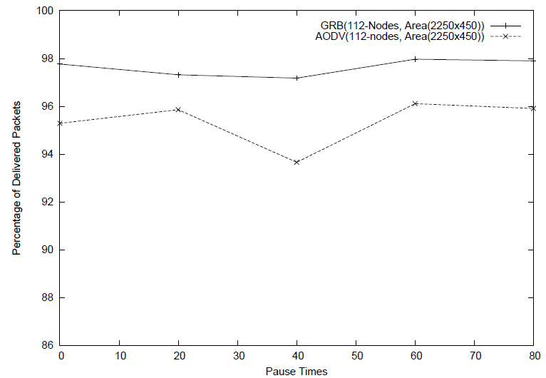
Figure 18: Packet Delivery Ratio of Network Area (2250x450), 112 nodes, 30-CBR Flows, GRB compared with AODV.

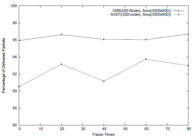
Figure 19: Packet Delivery Ratio of Network Area (3000x600), 200 nodes, 30-CBR Flows, GRB compared with AODV.

Figure 20: Packet Delivery Ratio of Network Area (2250x450), 112 nodes, 30-CBR Flows, GRB compared with DSR.

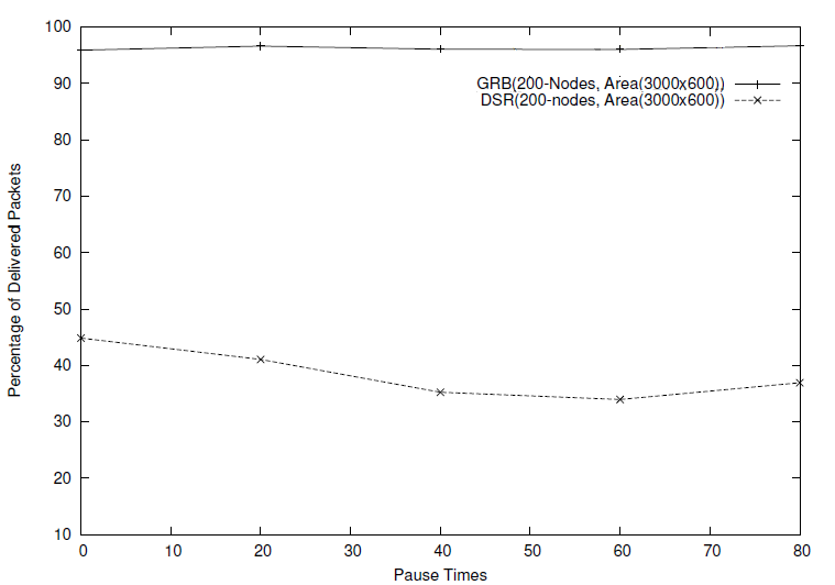
Figure 21: Packet Delivery Ratio of Network Area (3000x600), 200 nodes, 30-CBR Flows, GRB compared with DSR.

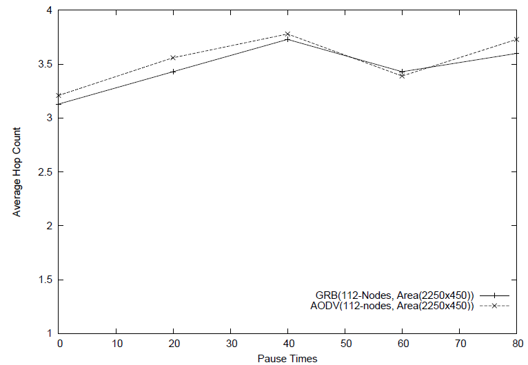
Figure 22: Average Hop Count of Network Area (2250x450), 112 nodes, 30-CBR Flows, GRB compared with AODV.

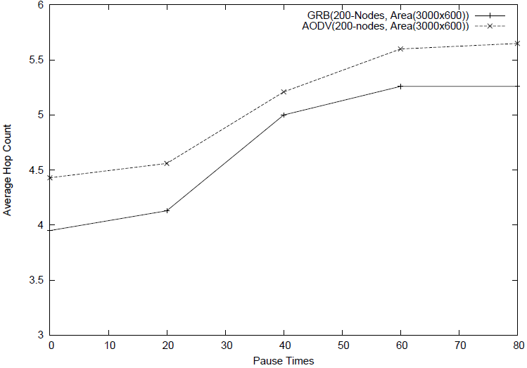
Figure 23: Average Hop Count of Network Area (3000x600), 200 nodes, 30-CBR Flows, GRB compared with AODV.

Table 4: Input Settings and Corresponding Results for both GRB and GPSR

Nodes	Network Area	PT(s)	SPDR(GRB)	SPDR(GPSR)
50	1500m X 300m	0	98.98	97.04
50	1500m X 300m	60	99.07	98.16
112	2250m X 450m	0	98.00	97.50
112	2250m X 450m	60	98.54	98.25
200	3000m X 600m	0	97.02	95.00
200	3000m X 600m	60	96.84	97.50

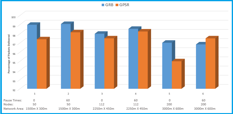
Figure 24: GRB Vs. GPSR.

4.5 GRB Vs. GPSR

Even though we didn’t simulate GPSR, we used the performance results published for GPSR in [8] and the results we obtained for GRB to compare the performance of the two protocols. As stated in [8], GPSR performance evaluation counts only those packets for which a path exists to the destination. We used the same input settings as those used for GPSR to compare the success rate. The settings are: 50 nodes, 30 CBR flows, pause times (PT) (0, 30, 60, and 120) seconds, area (1500x300) meters, and node density ($1node/9000m^{2}$). From the results presented in GPSR [8], successful packet delivery rate (SPDR) of GPSR ranges from 95% to 99.10% for pause time 0 second, while GRB successfully delivers 98.93% of the total packets sent. When pause time is 30 seconds, GPSR achieves success rates between 98.20% to 99.70% whereas GRB achieves a success rate of 99.33%. When pause time is 60 seconds, GPSR delivers from 98.70% to 99.40% of data packets sent, while GRB delivers 99.04% of all packets. Finally, when pause time is 120 seconds, GPSR’s packet delivery rate ranges from 98.60% to 99.40% and GRB’s packet delivery rate is 99.28%. The result of the comparison is shown in Table 4.

As shown in Figure 24, for 50 and 112 nodes, pause times 0 and 60 seconds, areas (1500x300) and (2250x450) meters, we see that GRB performs better than GPSR with respect to Successful Packet Delivery Ratio (SPDR). We noticed that the performance of our protocol in successfully delivering data packets is almost same as that of GPSR in some cases and higher than GPSR in other cases. However, when greedy routing fails due to a void in the direction of the destination, GPSR has to planarize the local network graph and use it to route around voids. Planarizing the graph results in computation overhead as well as routing failure. Figures 25, 26, and 27 show how GRB successfully routes around voids where GPSR could not because of the planarization and face routing problems discussed in Section 3.1. When face routing fails because of unidirectional links as shown in Figure 2, under GRB, the first packet follows the links labeled (1,2,3,4,5,6,7,8,9,10,11) to reach the destination as shown in Figure 25. However, the remaining packets will be routed via the links labeled (9,10,11) because the first packet backtracked from $V$ to $S$. Hence, in the Seen Table of the source $S$, it is stated that node $V$ is an invalid next hop for the destination $D$.

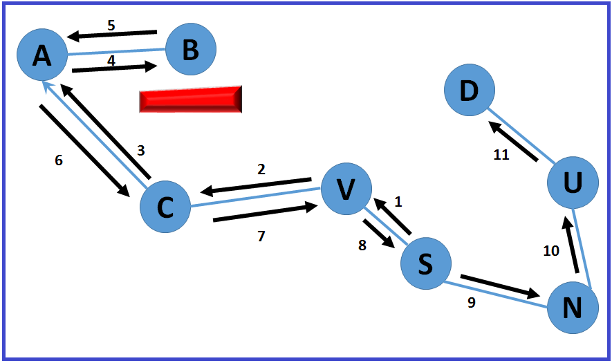
Figure 25: GRB Succeeds when Unidirectional Links Cause Routing Failure.

Figure 26: GRB Succeeds when Disconnected Links Cause Routing Failure.

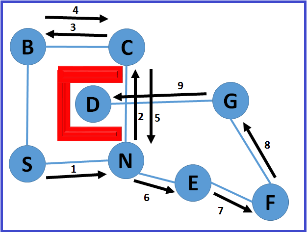
Figure 27: GRB Succeeds when Cross Links Cause Routing Failure.

When planarization of the local network graph results in disconnected links as shown in Figure 3, data packets under GRB follow the sold arrows (i.e. nodes (N,V,C)) to reach the destination $D$ as shown in Figure 26. When cross links caused data packets to loop as shown in Figure 4, the first packet follows the links labeled (1,2,3,4,5,6,7,8,9) under GRB as shown in Figure 27. Moreover, the remaining packets follow the path labeled (6,7,8,9) towards $D$.

GRB neither requires planarizarion of local network graph nor it switches from greedy mode to an alternative mode when a packet faces void; instead a node simply selects the best next hop without imposing the condition that the next hop be closer to the destination than itself. GRB depends on the Seen Table to determine the next hop. Therefore, GRB needs less control information which makes it better and robust. So, we can see the difference between GRB and GPSR in delivering data packets is around 0.0066% in one scenario keeping in mind that GRB outperforms GPSR in some other scenarios. When compared to the simplicity of GRB and the less control overhead GRB needs, this difference is negligible. It is worthy to recall that we select CBR flows randomly without knowing whether there exists a route corresponding to each flow. However, under GPSR, according to the authors: ”Only packets for which a path exists to the destination are included in the graph”.

5 Discussion

We note from the detailed description of the protocol Sect. 3 that data packets are forwarded greedily. When greedy forwarding fails, GRB picks the next best hop based on simple heuristics without incurring large computation overhead, unlike GPSR. A packet can come back (backtrack) to its sender/forwarder if the next hop picked for forwarding packet could not use any of its neighbors to forward the packet. If a packet backtracks from a neighbor selected as next hop, that next hop is recorded in the Seen Table; this prevents a node from selecting the same node as next hop when it has to forward succeeding packets to the same destination. Benefits of the Seen Table: (i) It prevents loops; (ii) after the first packet establishes the route to the destination, all the packets for the same source-destination pair follow the same route; (iii) it helps in decreasing hop count and latency.

6 Conclusion

In this paper, we presented GRB, a simple low-overhead position-based routing protocol which consistently and successfully delivers high percentage of data packets. We compared the performance of GRB with well known position-based protocol GPSR, the on-demand routing protocol AODV, and the Dynamic Source Routing (DSR) protocol. Our performance evaluation shows that GRB performs as good as GPSR (with low overhead) and better than AODV and DSR under most scenarios. Unlike GPSR, GRB does not need to construct planar graphs to route around voids; it simply picks the best next hop to forward the data packets, hence GRB is simple. On the other hand, it achieves comparable packet delivery ratio to GPSR and AODV, hence it is robust.

References

- [1] H. Li and M. Singhal, “An anchor-based routing protocol with cell id management system for ad hoc networks,” in Proceedings of International Conference on Computer Communications and Networks, Oct 2005.
- [2] H. Shen and L. Zhao, “Alert: An anonymous location-based efficient routing protocol in manets,” IEEE Transactions on Mobile Computing, vol. 12, no. 6, pp. 1079–1093, June 2013.
- [3] V. N. Talooki, H. Marques, and J. Rodriguez, “Energy efficient dynamic manet on-demand (e2dymo) routing protocol,” in Proceedings of International Symposium and Workshops on a World of Wireless, Mobile and Multimedia Networks (WoWMoM), June 2013.
- [4] K. Kavitha, K. Selvakumar, T. Nithya, and S. Sathyabama, “Zone based multicast routing protocol for mobile ad hoc network,” in Proceedings of International Conference on Emerging Trends in VLSI, Embedded System, Nano Electronics and Telecommunication System (ICEVENT), Jan 2013.
- [5] S. Jain, A. Shastri, and B. K. Chaurasia, “Analysis and feasibility of reactive routing protocols with malicious nodes in manets,” in Proceedings of International Conference on Communication Systems and Network Technologies (CSNT), April 2013.
- [6] J. Lin and G.-S. Kuo, “A novel location-fault-tolerant geographic routing scheme for wireless ad hoc networks,” in Proceedings of 63rd Vehicular Technology Conference, May 2006.
- [7] R. Flury and R. Wattenhofer, “Randomized 3d geographic routing,” in Proceedings of 27th IEEE international Conference on Computer Communications (INFOCOM), April 2008.
- [8] B. Karp and H. T. Kung, “Gpsr: Greedy perimeter stateless routing for wireless networks,” in Proceedings of the 6th Annual International Conference on Mobile Computing and Networking, 2000.
- [9] C. C. Hsu and C. L. Lei, “A geographic scheme with location update for ad hoc routing,” in Proceedings of Fourth International Conference on Systems and Networks Communications, ICSNC, Sept 2009.
- [10] V. C. Giruka and M. Singhal, “A self-healing on-demand geographic path routing protocol for mobile ad-hoc networks,” Ad Hoc Netw., vol. 5, no. 7, pp. 1113–1128, Sep. 2007.
- [11] C. E. Perkins and P. Bhagwat, “Highly dynamic destination-sequenced distance-vector routing (dsdv) for mobile computers,” SIGCOMM Comput. Commun. Rev., vol. 24, no. 4, pp. 234–244, Oct. 1994.
- [12] S. Basagni, I. Chlamtac, V. R. Syrotiuk, and B. A. Woodward, “A distance routing effect algorithm for mobility (dream),” in Proceedings of the 4th Annual ACM/IEEE International Conference on Mobile Computing and Networking (MobiCom), 1998.
- [13] Y. Zhao, Y. Chen, B. Li, and Q. Zhang, “Hop id: A virtual coordinate based routing for sparse mobile ad hoc networks,” IEEE Transactions on Mobile Computing, vol. 6, no. 9, pp. 1075–1089, 2007.
- [14] C. Lemmon, S. M. Lui, and I. Lee, “Geographic forwarding and routing for ad-hoc wireless network: A survey,” in Proceedings of Fifth International Joint Conference on INC, IMS and IDC. IEEE, 2009.
- [15] M. Shobana and S. Karthik, “A performance analysis and comparison of various routing protocols in manet,” in Proceedings of International Conference on Pattern Recognition, Informatics and Mobile Engineering (PRIME). IEEE, 2013.
- [16] F. Cadger, K. Curran, J. Santos, and S. Moffett, “A survey of geographical routing in wireless ad-hoc networks,” IEEE Communications Surveys & Tutorials, vol. 15, no. 2, pp. 621–653, 2013.
- [17] Y.-J. Kim, R. Govindan, B. Karp, and S. Shenker, “On the pitfalls of geographic face routing,” in Proceedings of the Joint Workshop on Foundations of Mobile Computing, ser. DIALM-POMC ’05. New York, NY, USA: ACM, 2005.
- [18] H. Frey and I. Stojmenovic, “On delivery guarantees of face and combined greedy-face routing in ad hoc and sensor networks,” in Proceedings of the 12th annual international conference on Mobile computing and networking. ACM, 2006.
- [19] B. Zhou, Y.-Z. Lee, and M. Gerla, “Direction assisted geographic routing for mobile ad hoc networks,” in Proceedings of MILCOM Military Communications Conference. IEEE, 2008.
- [20] M. Gerla, Y.-Z. Lee, B. Zhou, J. Chen, and A. Caruso, “Direction forwarding for highly mobile, large scale ad hoc networks,” in Challenges in Ad Hoc Networking. Springer, 2006, pp. 357–366.
- [21] G. Pei, M. Gerla, and T.-W. Chen, “Fisheye state routing: a routing scheme for ad hoc wireless networks,” in Proceedings of IEEE International Conference on Communications, 2000.
- [22] X. Li, N. Mitton, A. Nayak, and I. Stojmenovic, “Localized load-aware geographic routing in wireless ad hoc networks,” in Proceedings of IEEE International Conference on Communications (ICC), June 2012.
- [23] I. Stojmenovic, “Localized network layer protocols in wireless sensor networks based on optimizing cost over progress ratio,” IEEE Network, vol. 20, no. 1, pp. 21–27, Jan 2006.
- [24] A. Macintosh, M. Ghavami, M. F. Siyau, and S. Ling, “Local area network dynamic (landy) routing protocol: A position based routing protocol for manet,” in Proceedings of 18th European Wireless Conference. VDE, 2012.
- [25] C. E. Perkins and E. M. Royer, “Ad-hoc on-demand distance vector routing,” in Proceedings of Second IEEE Workshop on Mobile Computing Systems and Applications, WMCSA, Feb 1999.
- [26] D. B. Johnson and D. A. Maltz, “Dynamic source routing in ad hoc wireless networks,” in Mobile computing. Springer, 1996, pp. 153–181.
- [27] K. R. Gabriel and R. R. Sokal, “A new statistical approach to geographic variation analysis,” Systematic Biology, vol. 18, no. 3, pp. 259–278, 1969.
- [28] G. T. Toussaint, “The relative neighbourhood graph of a finite planar set,” Pattern recognition, vol. 12, no. 4, pp. 261–268, 1980.
- [29] X. Zeng, R. Bagrodia, and M. Gerla, “Glomosim: A library for parallel simulation of large-scale wireless networks,” SIGSIM Simul. Dig., vol. 28, no. 1, pp. 154–161, Jul. 1998. [Online]. Available: http://doi.acm.org/10.1145/278009.278027