Metriplectic Structure of a Radiation-Matter Interaction Toy Model

Abstract

A dynamical system defined by a metriplectic structure is a dissipative model characterized by a specific pair of tensors, which defines the Leibniz brackets. Generally, these tensors are Poisson brackets tensor and a symmetric metric tensor that models purely dissipative dynamics.

In this paper, the metriplectic system describing a simplified two-photon absorption by a two-level atom is disclosed. The Hamiltonian component describes the free electromagnetic radiation. The metric component encodes the radiation-matter coupling, driving the system to an asymptotically stable state in which the excited level of the atom is populated due to absorption.

This work is intended as a first result to pave the way to apply the metriplectic formalism to many other irreversible processes in nonlinear optics.

I Introduction

The modeling of irreversible systems is a fundamental issue in each physical field. Even though in quantum mechanics is a still debated topic, and many efforts have been done both in case of intrinsic irreversibility Marcucci and Conti (2016) and in open systems Garmon et al. (2012), classical mechanics boasts many more tools and much more established and recognized theories to describe time asymmetric phenomena. Nevertheless, when considering irreversibility due to dissipation, the study of metriplectic structures unveils a simple theory based on linear algebraic tools that have immediate thermodynamical translation, both in classical Turski (1987) and in quantum Turski (1996) systems.

In literature there are several examples of irreversible dynamics represented as metriplectic systems: from very simple systems in Newton’s mechanics Materassi and Tassi (2012a), to hydrodynamics Morrison (1984) and magneto-hydrodynamics Materassi and Tassi (2012b); more delicate, but extremely interesting, are the cases of kinetic equations, the collisional terms of which may be written as a semi-metric term, or that of a free rotator driven to a stable rotation axis by a suitably designed servo-engine Morrison (1986). In all the cases mentioned the non-Hamiltonian system gets gifted of the transparency of motions generated by Leibniz algebrae, even if proper symplectic formalism is not applicable; moreover, the energy landscape becomes tractable as the free energy is explicitly written.

The process of two-photon absorbtion (TPA) by a two-level atom is here described through a classical dynamical system, in which the energy initially located in the radiation variables is irreversibly converted into the energy pertaining to the population of the excited level. The final state, in which no free radiation exists any more while the excited state is populated, is the asymptotic equilibrium state of the system. The existence of asymptotically stable equilibrium makes the TPA similar to a dissipative process, like macroscopic friction, where an “ordered” form of energy is “consumed” in favour of the “internal energy” of some medium. This attitude describes the matter absorbing the electromagnetic wave energy as the environment of a system that would be Hamiltonian per se: the presence of the environment, with the matter-radiation interaction that “destroys” the radiation, breaks the Hamiltonian nature of the radiation dynamics. Such a scenario is described by the extension of the symplectic algebra of the Hamiltonian system to a metriplectic algebra of brackets Morrison (1986), where the Hamiltonian component of the motion is still given by the original Poisson bracket, while a suitable semi-defined metric bracket generates the non-Hamiltonian component. An extension of the Hamiltonian, namely the free energy of the system, represents the metriplectic generator of the motion. The foregoing program interprets the dynamics of classical dissipative systems as flows generated by a new kind of Leibniz algebrae of brackets Guha (2007), namely the metriplectic bracket.

This paper is organized as follow. In Section II we review the metriplectic formalism from a very general point of view. In Section III the dynamical variables are presented, together with the ODEs describing their evoulution in the presence of the dissipative interaction. Then, the dissipationless, i.e. Hamiltonian, limit is presented, in which the expression of the free radiation energy $H_{0}(q,p)$ works as a Hamiltonian and the population $n$ does not evolve. In Section IV the metriplectic algebra generating the non-Hamiltonian component of the dynamics is constructed: first of all, equations are composed to define the semi-metric tensor through which the metric bracket $\left(\cdot,\cdot\right)$ is defined; then, a completion energy $U(n)$ is constructed in order for $H_{0}(q,p)+U(n)$ to be constant along the non-Hamiltonian motion of the full system $(q,p,n)$. Finally, the framework is completed by defining the proper conditions on the entropy $S(n)$ and writing down the expression of the free energy $F(q,p,n)=H(q,p)+\chi S(n)$, being $H=H_{0}+U$ and the equilibrium points are determined as a consequence of this construction (in the sense that, choosing different expressions for $S(n)$, i.e. for $F(q,p,n)$, different equilibria $n_{\mathrm{eq}}$ are found). In Section V we summarize the results of our analysis. Details on the computation of the metric tensor $G$ are added in Appendix.

II General Metriplectic Formalism

Before describing how the metriplectic formalism is applied to the TPA, it is useful to sketch briefly the construction of a metriplectic system. Typically, one starts from a Hamiltonian system described by a set of variables $X$, the dynamics of which is generated by some Hamiltonian $H_{0}(X)$ and some Poisson bracket $\left\{\cdot,\cdot\right\}$ so that $\left(\dot{X}\right)_{0}=\left\{X,H_{0}(X)\right\}$ (the subscripts “0” refer to the dynamics generated by the sole $H_{0}$ via the bracket $\left\{\cdot,\cdot\right\}$). Then, some quantity $S$ is defined, with the property of being in involution with any possible function of $X$, $\left\{S,A\right\}=0\ \forall\ A(X)$, i.e. to be a Casimir of $\left\{\cdot,\cdot\right\}$: this quantity $S$ may either depend on the original variables $X$ only (as for the kinetic theories or for the rigid body), or on some “environmental” variable $Y$ too (as in the case of a particle motion with friction, or those of non-ideal hydrodynamics or magneto-hydrodynamics: this will be the case here too). The Casimir $S$ becomes the generator of a new non-Hamiltonian component of the motion, through the introduction of a new bracket, $\left(\cdot,\cdot\right)$, with properties of symmetry and semi-definiteness Morrison (1986): the extended system, based on the old Hamiltonian one, has now a new dynamics in which the variables $X$ evolve according to

$$\dot{X}=\left\{X,H\left(X,Y\right)\right\}+\chi\left(X,S\left(X,Y\right)\right),$$ (1)

while the motion of the environmental variables, if any, is typically influenced by $S$ and the metric bracket only:

$$\dot{Y}=\chi\left(Y,S\left(X,Y\right)\right).$$ (2)

In Eq. (1) the Hamiltonian $H(X,Y)$ may be different from the original $H_{0}(X)$, as it may include a term depending on $Y$ in order to close the system energetically, and take into account of the irreversible consumption of $H_{0}(X)$ (dissipation): the difference $U=H-H_{0}$ is the internal energy of the environment. In Eqs. (1, 2), the factor $\chi$ is a coefficient representing a coupling condition between $X$ and $Y$, or characterizing the asymptotically stable equilibrium; the strength of the dissipative interaction, defining the non-dissipative (Hamiltonian) regime in some suitable limit of its, is some $\alpha$ included in the definition of $\left(\cdot,\cdot\right)$, so that $\alpha\rightarrow 0$ turns off dissipation. One may well say:

$$\lim_{\alpha\rightarrow 0}\dot{X}=\left\{X,H_{0}\left(X,Y\right)\right\},\ \ \lim_{\alpha\rightarrow 0}\dot{Y}=0.$$ (3)

(from Eq. (1, 2) it appears that also the limit for $\chi\rightarrow 0$ gives the ODEs in Eq. (3); however, this does not switch off dissipation, but simply describes a condition in which it is uneffective, see Sections IV and V).

As far as the bracket $\left(\cdot,\cdot\right)$ and the Casimir $S$ are concerned, the semi-definiteness of the first one, $\left(A,B\right)\leq 0\ \forall\ A,B$, and a suitable choice of the sign of $\chi$, i.e. $\chi<0$, implies that $S$ will grow monotonically along the system motion $\dot{S}\geq 0$, until some asymptotically stable equilibrium $Z_{\mathrm{eq}}=(X_{\mathrm{eq}},Y_{\mathrm{eq}})$ is reached, so that $\dot{S}(Z_{\mathrm{eq}})=0$ Morrison (1986). In other words, the Casimir $S$ turns out to be a Lyapunov function around $Z_{\mathrm{eq}}$, and it can be understood as a form of entropy Materassi (2016) (of course, all the reasoning just presented is rephrased “without $Y$” for those metriplectic systems in which no “environment” needs to be defined).

In order to complete the picture, the property $\left(H,A\right)=0\ \forall\ A$ is requested for the metric bracket and the total Hamiltonian $H$, in order for dissipation not to “delete” the total energy, but just transform it. It must be underlined that this construction does not include “all” the dynamical systems referred to as “metriplectic” in literature: this is the construction of a complete metriplectic system (CMS), while incomplete metriplectic systems (IMS) may be defined too, with the two brackets but the Hamiltonian as the only generator. IMS are suitable to describe energetically open systems Turski (1987).

The development presented here makes the TPA process tractable in a very transparent way as a CMS, and points towards the systematic algebrization of non-linear optics.

The system introduced here in order to turn the TPA process into a CMS has three degrees of freedom: radiation is represented either via a complex phasor $\psi$, or a couple of real variables $(q,p)$; the population of the excited level is given by some real variable $n$. During the irreversible process, the electromagnetic energy $H_{0}(q,p)$ is converted into the energy $U(n)$ associated with $n\neq 0$. In our “metriplectization” scheme one starts from the equations of motion of the state $Z=(q,p,n)$ and observes that a suitable limit of them reduces the system to a Hamiltonian one. In this Hamiltonian limit a Poisson bracket is defined, so that $q$ and $p$ are canonically conjugated $\left\{q,p\right\}=1$, while $n$ remains apparently outside the play as $\left\{n,q\right\}=\left\{n,p\right\}=0$. Indeed, the population of the excited level is in involution with $q$ and $p$, so that any function $S(n)$ will be a Casimir for $\left\{\cdot,\cdot\right\}$. The program then is to find a suitable function $H_{0}(q,p)$ that may play the role of Hamiltonian in the Hamiltonian limit: this represents the free radiation energy, to be extended as $H(q,p,n)=H_{0}(q,p)+U(n)$ to include the energy pertaining to the filling of the excited state, namely the internal energy of the environment “atoms”. In order to complete the metriplectic framework, suitable forms for $S(n)$ and for the metric bracket $\left(\cdot,\cdot\right)$ must be constructed, and this is essentially what is done in the present work.

III Two-Photon Absorption Toy Model

We consider a very simplified toy model for the two-level atomic system Boyd (2008); Moloney and Newell (2004). The TPA, sketched in Fig. (1), is expressed by the following differential equations:

$$\left\{\begin{array}[]{l}\dot{\psi}=\imath|\psi|^{2}\psi-\alpha n\psi\\ \dot{n}=\frac{k}{2}|\psi|^{4}\end{array}\right.,$$ (4)

being $\psi$ the complex field amplitude, $n$ the population of second level, $k>0$ and $\alpha>0$. This system is directly derived by the multi-photon absorption model Feng et al. (1997); Mlejnek et al. (1998); Schwarz et al. (2000), when neglecting several physical phenomena, e.g., the spontaneous emission. Moving to real-valued functions, we define

$$\psi=\frac{q-\imath p}{\sqrt{2}},$$ (5)

so that in terms of the variables $q$ and $p$ the system (4) reads:

$$\left\{\begin{array}[]{l}\dot{q}=\frac{1}{2}p(q^{2}+p^{2})-\alpha nq\\ \dot{p}=-\frac{1}{2}q(q^{2}+p^{2})-\alpha np\\ \dot{n}=\frac{k}{8}(q^{2}+p^{2})^{2}\end{array}\right..$$ (6)

It is useful to observe that, in the limit

$$\alpha\rightarrow 0,\;k\rightarrow 0$$ (7)

Eqs. (6) become a Hamiltonian system, so that the conditions (7) will be referred to as non-dissipative limit (NDL); under these conditions, the ODEs in $q$ and $p$ read:

$$\left\{\begin{array}[]{l}\dot{q}=\frac{1}{2}p(q^{2}+p^{2})\\ \dot{p}=-\frac{1}{2}q(q^{2}+p^{2})\\ \dot{n}=0\end{array}\right..$$ (8)

As one defines the Hamiltonian

$$H_{0}=\frac{1}{2}\left(\frac{q^{2}+p^{2}}{2}\right)^{2}.$$ (9)

and the Poisson bracket

$$\left\{q,p\right\}=1,\ \left\{q,n\right\}=0,\ \left\{p,n\right\}=0,$$ (10)

any quantity $f\left(q,p,n\right)$ evolves according to:

$$\dot{f}=\left\{f,H_{0}\right\}$$

along the motion (8). The quantity defined in Eq. (9) turns out to be the energy that can be attributed to the free radiation as it is not interacting with matter.

The dissipative nature of the dynamical system (6) emerges as one sees that the following relationships hold

$$\dot{H}_{0}=-4\alpha nH_{0},\ \dot{n}=kH_{0}$$ (11)

as $\alpha$ and $k$ are positive constants, and as long as $n\geq 0$, this means that $\dot{H_{0}}\leq 0$ and $\dot{n}\geq 0$; all in all, the system of Eqs. (11), that are equivalent to Eqs. (6), simply describe the consumption of $H_{0}$ in favour of the quantity $n$. The system (6) has an energy dynamics similar to classical dissipation, that points towards the formulation of it as a complete metriplectic system Materassi (2016).

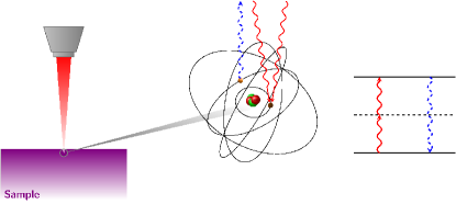
Figure 1: Pictorial sketch of absorbtion of two photons in a two-level atom. In our system, Eq. (4) does not have terms of spontaneous emission, considered negligible. This is here represented by the dashed blue line, not present in our model.

IV Metriplectic Formulation

In order to recognize a CMS equivalent to Eqs. (6), let us put those ODEs in the general form of a Hamiltonian system “perturbed” by dissipative terms, the most general form of which reads:

$$\left\{\begin{array}[]{l}\dot{q}=\{q,H\}+\psi_{q}\\ \dot{p}=\{p,H\}+\psi_{p}\\ \dot{n}=\{n,H\}+\psi_{n}\end{array}\right.,$$ (12)

with $H(p,q,n)$ the total Hamiltonian, $\{f,g\}=J^{ij}\partial_{i}f\partial_{j}g$ the Poisson brackets (PB) with

$$J^{ij}=\left(\begin{array}[]{ccc}0&1&0\\ -1&0&0\\ 0&0&0\end{array}\right),$$ (13)

and improperly $i,j=q,p,n$. Seeing that $\{n,A\}=0$ for any observable $A(q,p,n)$ is straightforward from Eq. (13). This implies that any function $\mathcal{C}(n)$ is a Casimir; indeed, $\{\mathcal{C}(n),H_{0}\}=\mathcal{C}^{\prime}(n)\{n,H_{0}\}=0$, so that one has:

$$(\ref{eq:nndiss})\Rightarrow\dot{C}\left(n\right)=0.$$

In order to express Eq. (12) as a metriplectic system Materassi (2015, 2016), we define the metric brackets $(f,g)=G^{ij}\partial_{i}f\partial_{j}g$, constructing

$$G^{ij}=\left(\begin{array}[]{ccc}G^{qq}&G^{qp}&G^{qn}\\ G^{qp}&G^{pp}&G^{pn}\\ G^{qn}&G^{pn}&G^{nn}\end{array}\right)$$ (14)

as a symmetric, positive semi-definite matrix.

Eq. (12) will be put in the form of

$$\left\{\begin{array}[]{l}\dot{q}=\{q,H\}+\chi(q,S)\\ \dot{p}=\{p,H\}+\chi(p,S)\\ \dot{n}=\chi(n,S)\end{array}\right.,$$ (15)

where $\chi$ is a constant to be calculated once the desired $Z_{\mathrm{eq}}$ is defined. For the moment being, $\chi=\pm 1$ may be understood. Indeed, once defined the metriplectic (or Leibniz) brackets

$$<<f,g>>:=\{f,g\}+(f,g),$$ (16)

the entropy $S(q,p,n)$ and the free energy $F=H+\chi S$, if $\nabla S\in Ker(J)$ and $\nabla H\in Ker(G)$, namely,

$$J^{ij}\partial_{j}S=G^{ij}\partial_{j}H=0,$$ (17)

then

$$\dot{g}=<<g,F>>=\{g,H\}+\chi(g,S).$$ (18)

Eq. (17) implies that the entropy is a mere function of $n$.

IV.1 The Metric Brackets Tensor

Thanks to Eq. (17), the system in Eq. (15) becomes

$$\left\{\begin{array}[]{l}\dot{q}=\partial_{p}H+\chi G^{qn}S^{\prime}(n)\\ \dot{p}=\partial_{q}H+\chi G^{pn}S^{\prime}(n)\\ \dot{n}=\chi G^{nn}S^{\prime}(n)\end{array}\right.,$$ (19)

therefore our overriding concern is to determine the tensor $G$. In order to obtain such a result, we follow a linear algebraic procedure. Calculations are illustrated item by item in Appendix. The final result is:

$$G_{\mathbb{E}}^{qq}=\frac{\partial_{q}H\partial_{n}H\left[b\partial_{q}H\partial_{n}H+2c\partial_{p}H\sqrt{(\partial_{q}H)^{2}+(\partial_{p}H)^{2}+(\partial_{n}H)^{2}}\right]}{\left[(\partial_{q}H)^{2}+(\partial_{p}H)^{2}\right]\left[(\partial_{q}H)^{2}+(\partial_{p}H)^{2}+(\partial_{n}H)^{2}\right]},$$

$$G_{\mathbb{E}}^{qp}=\frac{\partial_{n}H\left[b\partial_{q}H\partial_{p}H\partial_{n}H+c\left[(\partial_{p}H)^{2}-(\partial_{q}H)^{2}\right]\sqrt{(\partial_{q}H)^{2}+(\partial_{p}H)^{2}+(\partial_{n}H)^{2}}\right]}{\left[(\partial_{q}H)^{2}+(\partial_{p}H)^{2}\right]\left[(\partial_{q}H)^{2}+(\partial_{p}H)^{2}+(\partial_{n}H)^{2}\right]},$$

$$G_{\mathbb{E}}^{qn}=-\frac{b\partial_{q}H\partial_{n}H+c\partial_{p}H\sqrt{(\partial_{q}H)^{2}+(\partial_{p}H)^{2}+(\partial_{n}H)^{2}}}{(\partial_{q}H)^{2}+(\partial_{p}H)^{2}+(\partial_{n}H)^{2}},$$

$$G_{\mathbb{E}}^{pp}=\frac{b(\partial_{p}H)^{2}(\partial_{n}H)^{2}-2c\partial_{q}H\partial_{p}H\partial_{n}H\sqrt{(\partial_{q}H)^{2}+(\partial_{p}H)^{2}+(\partial_{n}H)^{2}}}{\left[(\partial_{q}H)^{2}+(\partial_{p}H)^{2}\right]\left[(\partial_{q}H)^{2}+(\partial_{p}H)^{2}+(\partial_{n}H)^{2}\right]},$$

$$G_{\mathbb{E}}^{pn}=\frac{-b\partial_{p}H\partial_{n}H+c\partial_{q}H\sqrt{(\partial_{q}H)^{2}+(\partial_{p}H)^{2}+(\partial_{n}H)^{2}}}{(\partial_{q}H)^{2}+(\partial_{p}H)^{2}+(\partial_{n}H)^{2}},$$

$$G_{\mathbb{E}}^{nn}=\frac{b\left[(\partial_{q}H)^{2}+(\partial_{p}H)^{2}\right]}{(\partial_{q}H)^{2}+(\partial_{p}H)^{2}+(\partial_{n}H)^{2}},$$

with

$$\left\{\begin{array}[]{l}b=\chi\frac{\psi_{n}}{S^{\prime}(n)}\frac{(\partial_{q}H)^{2}+(\partial_{p}H)^{2}+(\partial_{n}H)^{2}}{(\partial_{q}H)^{2}+(\partial_{p}H)^{2}}\\ c=\chi\frac{\psi_{p}\partial_{q}H-\psi_{q}\partial_{p}H}{S^{\prime}(n)}\frac{\sqrt{(\partial_{q}H)^{2}+(\partial_{p}H)^{2}+(\partial_{n}H)^{2}}}{(\partial_{q}H)^{2}+(\partial_{p}H)^{2}}\end{array}\right..$$ (20)

With reference to the Appendix, one attains a third equation from Eq. (32), namely,

$$\psi_{q}\partial_{q}H+\psi_{p}\partial_{p}H+\psi_{n}\partial_{n}H=0.$$ (21)

This last condition expresses the conservation of the Hamiltonian $H$ when the relationships (32) are enforced, that is precisely what is required by theory.

IV.2 The Total Hamiltonian

Considering Eq. (6), we fix

$$\left\{\begin{array}[]{l}\psi_{q}=-\alpha nq\\ \psi_{p}=-\alpha np\\ \psi_{n}=\frac{k}{8}(q^{2}+p^{2})^{2}\end{array}\right.,$$ (22)

therefore $\partial_{q}H=\frac{1}{2}q(q^{2}+p^{2})$ and $\partial_{p}H=\frac{1}{2}p(q^{2}+p^{2})$, which imply that the total Hamiltonian reads:

$$H(q,p,n)=H_{0}(q^{2}+p^{2})+U(n),$$ (23)

being $H_{0}(q^{2}+p^{2})$ the free radiation Hamiltonian defined in Eq. (9). In order to determine $U(n)$, we need to take into account Eq. (21):

$$-\alpha nq\frac{1}{2}q(q^{2}+p^{2})-\alpha np\frac{1}{2}p(q^{2}+p^{2})+\frac{k}{8}(q^{2}+p^{2})^{2}U^{\prime}(n)=0,$$ (24)

whence

$$U(n)=\frac{2\alpha}{k}n^{2}+U_{0}.$$ (25)

IV.3 Entropy and Equilibrium States

We are now in the position of writing explicitely the free energy $F$

$$F(q^{2}+p^{2},n)=H_{0}(q^{2}+p^{2})+U(n)+\chi S(n).$$

As the expression (25) is used, one has

$$F\left(q^{2}+p^{2},n\right)=\frac{1}{8}\left(q^{2}+p^{2}\right)^{2}+\frac{2\alpha}{k}n^{2}+U_{0}+\chi S\left(n\right).$$ (26)

EQuiLiBrium states of the system must satisfy the condition

$$\delta F=\partial_{q}F\delta q+\partial_{p}F\delta p+\partial_{n}F\delta n=0,$$ (27)

that is:

$$q_{eq}=p_{eq}=0,\;\;S^{\prime}(n)|_{n_{eq}}=-\chi\frac{4\alpha}{k}n_{eq}.$$ (28)

As expected, different entropy functions correspond to different equilibrium points.

Some lines ago we anticipated that $\chi\rightarrow 0$ suppresses the metric part of the dynamics: indeed here one sees that, in this limit, the equilibrium value of $n$ vanishes:

$$\lim_{\chi\rightarrow 0}n_{\mathrm{eq}}=0.$$

This means putting oneself in the condition of an equilibrium reached without populating the atomic excited level (e.g., at $0{{}^{\circ}}K$ temperature), that does not mean turning off the matter-radiation coupling.

Before going to the conclusions, it is important to note that $\alpha$ and $k$ appear everywhere as a ratio: it would make sense to introduce an always finite constant $\kappa$ so that $k=\kappa\alpha$. This would reduce the non-dissipative condition (7) to the much simpler $\alpha\rightarrow 0$, that is, again, a statement about interactions, while $\chi\rightarrow 0$ would be a statement about the equilibrium around which we are working.

V Conclusions

This work applies the metriplectic theory and Leibniz algebrae to a dissipative nonlinear optical phenomenon: the two-photon absorption by a two-level atom with negligible spontaneous emission. Once the physical problem was formulated in terms of the conservative part $H_{0}$ of the total Hamiltonian $H$, the metric tensor $G$ and the metriplectic brackets $<<\cdot,\cdot>>$, we have found the mathematical expression of $H$ as function of the dynamical variables $q,p,n$. In particular, we have found the dissipative part $U$ of $H$, which depends only on the second level population $n$. We have also found the free energy $F$ and the equilibrium states, varying with the definition of entropy, as expected.

We believe that this manuscript opens the way to an ambitious research program in which the metriplectic formalism is used to explore irreversibility in nonlinear optics.

VI Acknowledgments

C.C. and G.M. acknowledge support from the Templeton Foundation (grant number 58277), the H2020 QuantERA project QUOMPLEX (project ID 731473) and PRIN project NEMO (ref. 2015KEZNYM). They also acknowledge I. M. Deen for technical support with the computational resources.

Appendix

Here we determine the tensor $G$. We start from Eq. (17) and look for an orthornormal basis $\mathbb{B}:=(\hat{n}_{1},\hat{n}_{2},\hat{n}_{3})$, with $\hat{n}_{3}=\frac{\nabla H}{||\nabla H||}$, through a standard Gram-Schmidt process. We find

$$\hat{n}_{1}=\left(\begin{array}[]{c}-\frac{\partial_{p}H}{\sqrt{(\partial_{q}H)^{2}+(\partial_{p}H)^{2}}}\\ \frac{\partial_{q}H}{\sqrt{(\partial_{q}H)^{2}+(\partial_{p}H)^{2}}}\\ 0\end{array}\right),\;\hat{n}_{2}=\left(\begin{array}[]{c}-\frac{\partial_{q}H\partial_{n}H}{\sqrt{(\partial_{q}H)^{2}+(\partial_{p}H)^{2}}\sqrt{(\partial_{q}H)^{2}+(\partial_{p}H)^{2}+(\partial_{n}H)^{2}}}\\ -\frac{\partial_{p}H\partial_{n}H}{\sqrt{(\partial_{q}H)^{2}+(\partial_{p}H)^{2}}\sqrt{(\partial_{q}H)^{2}+(\partial_{p}H)^{2}+(\partial_{n}H)^{2}}}\\ \sqrt{\frac{(\partial_{q}H)^{2}+(\partial_{p}H)^{2}}{(\partial_{q}H)^{2}+(\partial_{p}H)^{2}+(\partial_{n}H)^{2}}}\end{array}\right),\;\hat{n}_{3}=\left(\begin{array}[]{c}\frac{\partial_{q}H}{\sqrt{(\partial_{q}H)^{2}+(\partial_{p}H)^{2}+(\partial_{n}H)^{2}}}\\ \frac{\partial_{p}H}{\sqrt{(\partial_{q}H)^{2}+(\partial_{p}H)^{2}+(\partial_{n}H)^{2}}}\\ \frac{\partial_{n}H}{\sqrt{(\partial_{q}H)^{2}+(\partial_{p}H)^{2}+(\partial_{n}H)^{2}}}\end{array}\right).$$ (29)

Then, we move from basis $\mathbb{B}$ to the canonical basis $\mathbb{E}=(\hat{e}_{1},\hat{e}_{2},\hat{e}_{3})$, $\hat{e}_{j}=(\delta_{ij})^{t}_{i=1,2,3}$, by defining the unitary change of basis matrix

$$C=\left(\begin{array}[]{ccc}-\frac{\partial_{p}H}{\sqrt{(\partial_{q}H)^{2}+(\partial_{p}H)^{2}}}&-\frac{\partial_{q}H\partial_{n}H}{\sqrt{(\partial_{q}H)^{2}+(\partial_{p}H)^{2}}\sqrt{(\partial_{q}H)^{2}+(\partial_{p}H)^{2}+(\partial_{n}H)^{2}}}&\frac{\partial_{q}H}{\sqrt{(\partial_{q}H)^{2}+(\partial_{p}H)^{2}+(\partial_{n}H)^{2}}}\\ \frac{\partial_{q}H}{\sqrt{(\partial_{q}H)^{2}+(\partial_{p}H)^{2}}}&-\frac{\partial_{p}H\partial_{n}H}{\sqrt{(\partial_{q}H)^{2}+(\partial_{p}H)^{2}}\sqrt{(\partial_{q}H)^{2}+(\partial_{p}H)^{2}+(\partial_{n}H)^{2}}}&\frac{\partial_{p}H}{\sqrt{(\partial_{q}H)^{2}+(\partial_{p}H)^{2}+(\partial_{n}H)^{2}}}\\ 0&\sqrt{\frac{(\partial_{q}H)^{2}+(\partial_{p}H)^{2}}{(\partial_{q}H)^{2}+(\partial_{p}H)^{2}+(\partial_{n}H)^{2}}}&\frac{\partial_{n}H}{\sqrt{(\partial_{q}H)^{2}+(\partial_{p}H)^{2}+(\partial_{n}H)^{2}}}\end{array}\right),$$ (30)

whence

$$C^{-1}=C^{t}\mbox{ and }\mathbb{B}=\mathbb{E}C.$$

On $\mathbb{E}$, the tensor $G$ is expressed in Eq. (14), but, in order to obey Eq. (17), on $\mathbb{B}$ it must be $\nabla H$-transverse, that is,

$$G_{\mathbb{B}}=\left(\begin{array}[]{ccc}a&c&0\\ c&b&0\\ 0&0&0\end{array}\right),$$ (31)

with $a,b,c\in\mathbb{R}$ and $ab-c^{2}\neq 0$. Since $G_{\mathbb{E}}=CG_{\mathbb{B}}C^{t}$, it turns out that

$$G_{\mathbb{E}}^{qq}=\frac{a(\partial_{p}H)^{2}\left[(\partial_{q}H)^{2}+(\partial_{p}H)^{2}+(\partial_{n}H)^{2}\right]+\partial_{q}H\partial_{n}H\left[b\partial_{q}H\partial_{n}H+2c\partial_{p}H\sqrt{(\partial_{q}H)^{2}+(\partial_{p}H)^{2}+(\partial_{n}H)^{2}}\right]}{\left[(\partial_{q}H)^{2}+(\partial_{p}H)^{2}\right]\left[(\partial_{q}H)^{2}+(\partial_{p}H)^{2}+(\partial_{n}H)^{2}\right]},$$

$$G_{\mathbb{E}}^{qp}=\frac{-a\partial_{q}H\partial_{p}H\left[(\partial_{q}H)^{2}+(\partial_{p}H)^{2}+(\partial_{n}H)^{2}\right]+\partial_{n}H\left[b\partial_{q}H\partial_{p}H\partial_{n}H+c\left[(\partial_{p}H)^{2}-(\partial_{q}H)^{2}\right]\sqrt{(\partial_{q}H)^{2}+(\partial_{p}H)^{2}+(\partial_{n}H)^{2}}\right]}{\left[(\partial_{q}H)^{2}+(\partial_{p}H)^{2}\right]\left[(\partial_{q}H)^{2}+(\partial_{p}H)^{2}+(\partial_{n}H)^{2}\right]},$$

$$G_{\mathbb{E}}^{qn}=-\frac{b\partial_{q}H\partial_{n}H+c\partial_{p}H\sqrt{(\partial_{q}H)^{2}+(\partial_{p}H)^{2}+(\partial_{n}H)^{2}}}{(\partial_{q}H)^{2}+(\partial_{p}H)^{2}+(\partial_{n}H)^{2}},$$

$$G_{\mathbb{E}}^{pp}=\frac{b(\partial_{p}H)^{2}(\partial_{n}H)^{2}+\partial_{q}H\left\{-2c\partial_{p}H\partial_{n}H\sqrt{(\partial_{q}H)^{2}+(\partial_{p}H)^{2}+(\partial_{n}H)^{2}}+a\partial_{q}H\left[(\partial_{q}H)^{2}+(\partial_{p}H)^{2}+(\partial_{n}H)^{2}\right]\right\}}{\left[(\partial_{q}H)^{2}+(\partial_{p}H)^{2}\right]\left[(\partial_{q}H)^{2}+(\partial_{p}H)^{2}+(\partial_{n}H)^{2}\right]},$$

$$G_{\mathbb{E}}^{pn}=\frac{-b\partial_{p}H\partial_{n}H+c\partial_{q}H\sqrt{(\partial_{q}H)^{2}+(\partial_{p}H)^{2}+(\partial_{n}H)^{2}}}{(\partial_{q}H)^{2}+(\partial_{p}H)^{2}+(\partial_{n}H)^{2}},$$

$$G_{\mathbb{E}}^{nn}=\frac{b\left[(\partial_{q}H)^{2}+(\partial_{p}H)^{2}\right]}{(\partial_{q}H)^{2}+(\partial_{p}H)^{2}+(\partial_{n}H)^{2}}.$$

By comparing Eq. (12) and Eq. (19), we get

$$\left\{\begin{array}[]{l}G^{qn}=\chi\frac{\psi_{q}}{S^{\prime}(n)}\\ G^{pn}=\chi\frac{\psi_{p}}{S^{\prime}(n)}\\ G^{nn}=\chi\frac{\psi_{q}}{S^{\prime}(n)}\end{array}\right.,$$ (32)

which is indepedent of $a$: hence we may fix $a=0$ without loss of generality. Finally, we solve Eq. (32) for the parameter $b,c$, and obtain Eq. (20).

References

• Marcucci and Conti (2016) G. Marcucci and C. Conti, Phys. Rev. A 94, 052136 (2016).
• Garmon et al. (2012) S. Garmon, T. Petrosky, L. Simine,  and D. Segal, Fortschritte der Physik 61, 261 (2012).
• Turski (1987) L. A. Turski, Physics Letters A 125, 461 (1987).
• Turski (1996) L. A. Turski, in From Quantum Mechanics to Technology, edited by Z. Petru, J. Przystawa,  and K. Rapcewicz (Springer Berlin Heidelberg, Berlin, Heidelberg, 1996).
• Materassi and Tassi (2012a) M. Materassi and E. Tassi, Intellectual Archive 1, 45 (2012a).
• Morrison (1984) P. J. Morrison, Physics Letters A 100, 423 (1984).
• Materassi and Tassi (2012b) M. Materassi and E. Tassi, Physica D 241, 729 (2012b).
• Morrison (1986) P. J. Morrison, Physica D 18, 410 (1986).
• Guha (2007) P. Guha, Journal of Mathematical Analysis and Applications 326, 121 (2007).
• Materassi (2016) M. Materassi, Entropy 18, 304 (2016).
• Boyd (2008) R. W. Boyd, Nonlinear Optics, 3rd ed. (Academic Press, Burlington, 2008).
• Moloney and Newell (2004) J. Moloney and A. Newell, Nonlinear Optics, Advanced Book Program (Avalon Publishing, 2004).
• Feng et al. (1997) Q. Feng, J. V. Moloney, A. C. Newell, E. M. Wright, K. Cook, P. K. Kennedy, D. X. Hammer, B. A. Rockwell,  and C. R. Thompson, IEEE Journal of Quantum Electronics 33, 127 (1997).
• Mlejnek et al. (1998) M. Mlejnek, E. M. Wright,  and J. V. Moloney, Opt. Lett. 23, 382 (1998).
• Schwarz et al. (2000) J. Schwarz, P. Rambo, J.-C. Diels, M. Kolesik, E. M. Wright,  and J. V. Moloney, Optics Communications 180, 383 (2000).
• Materassi (2015) M. Materassi, Entropy 17, 1329 (2015).