Dispatching to Parallel Servers

Abstract

Policy iteration techniques for multiple-server dispatching rely on the computation of value functions. In this context, we consider the continuous-space M/G/1-FCFS queue endowed with an arbitrarily-designed cost function for the waiting times of the incoming jobs. The associated value function is a solution of Poisson’s equation for Markov chains, which in this work we solve in the Laplace transform domain by considering an ancillary, underlying stochastic process extended to (imaginary) negative backlog states. This construction enables us to issue closed-form value functions for polynomial and exponential cost functions and for piecewise compositions of the latter, in turn permitting the derivation of interval bounds for the value function in the form of power series or trigonometric sums. We review various cost approximation schemes and assess the convergence of the interval bounds these induce on the value function. Namely: Taylor expansions (divergent, except for a narrow class of entire functions with low orders of growth), and uniform approximation schemes (polynomials, trigonometric), which achieve optimal convergence rates over finite intervals. This study addresses all the steps to implementing dispatching policies for systems of parallel servers, from the specification of general cost functions towards the computation of interval bounds for the value functions and the exact implementation of the first-policy improvement step.

I Introduction

An essential design aspect for systems of parallel servers resides in the allocation of the processing resources to the impending workload. In the allocation problem, commonly referred to as dispatching (also: task assignment or routing), one server must be assigned to each incoming job in a way so as to minimize a performance metric of interest: parallel computing (mobile cloud computing, server clusters, supercomputers), industrial logistics (customer service systems), and traffic congestion management (visitor queues, road tolls).

Figure 1: Size-aware dispatching with i.i.d. service times ($X_{n}\overset{d}{=}X$ for all $n$) and i.i.d. inter-arrival times ($T_{n}\sim\textup{Exp}({\lambda})$ for all $n$) to $k$ M/G/1-FCFS servers with backlog $u=(u_{1},\dots,u_{k})$.

We are interested in sytems composed of several first-come, first-served (FCFS) queueing servers operated in parallel, and fed with a sequence of jobs with Markovian arrival times. In our model, illustrated in Figure 1, every new job turning up at the dispatcher is instantly forwarded towards one of the servers, where a penalty is incurred as a function of the backlog (uncompleted work) at the server upon job arrival—server backlog thus coinciding with the waiting time of the job until processing begins. Our objective is to minimize the average cost experienced by the system over an infinite time horizon.

A standard approach for solving this problem is through policy iteration (PI), howard60 ; bertsekas07 . Starting with an inital dispatching policy, PI proceeds in two steps, repeated in turn until a fixed policy is reached: (i) policy evaluation, where the mean cost of the considered policy is computed, together with a value function expressing state sensitivity with respect to the steady-state costs induced by the policy; followed by (ii) policy improvement, where the value function is exploited to improve the current policy and derive a new, more cost-effective dispatching policy. The policy evaluation step is difficult to implement in continuous state spaces without extensive Monte Carlo simulations. Only the first PI iteration on a tractable, random initial policy is easier to carry out, because the job flow then decomposes into independent Poisson processes for the individual queueing servers, and the value function takes a separable form, solution of the so-called Poisson equation. The first-policy improvement (FPI) approach (also known as one-step policy iteration, and variants) consists of cutting short the policy iteration algorithm after the first iteration. The motivation behind first-policy improvement (FPI) is twofold: it is known that a single iteration of the PI algorithm may produce fine heuristics (see e.g. krishnan87 ; wijngaard79 ; ott92 ; sassen97 ; bhulai06 or (tijms03, , §7.5)) and, besides, the Poisson equation for Markov chains admits explicit solutions readily available for effortless  policy iteration (PI).

Related work and our contribution. The existence of explicit solutions to the Poisson equation for the waiting times of the M/G/1 queue was pointed out in glynn94 , where a general solution to Poisson’s equation was proposed in the form of a fundamental kernel, whose application to the cost function produces solutions of the equation. These solutions proved, in particular, to take closed forms for cost functions given as moments of the waiting time, $f(u)=u^{n}$. There followed a list of derivations of explicit value functions for Markovian queueing systems: both in discrete-space settings where only the number of yet unprocessed jobs at the servers is known to the dispatcher and (typically) the expected sojourn times of the incoming jobs are penalized, krishnan87 ; sassen97 ; bhulai03 ; bhulai06 ; and in ‘size-aware’ continuous-space settings where the service times of the jobs become available to the dispatcher upon arrival and the actual waiting or sojourn times are penalized, Aalto96NTS ; hyytia11MM1PS ; hyytia12OnTheVF ; hyytia-ejor-2012 ; hyytia14TaskAssignment . Recent studies on size-aware dispatching renewed the interest in explicit Poisson solutions, extending their class in hyytia-peva-2017 to the fixed-deadline cost functions $f(u)=\mathbf{1}_{[\tau,\infty)}(u)$, and to exponential costs in hyytia-peva-2020 , with views on polynomials. In the discrete space setting, the forms $f[u]=u^{n}a^{-u}$ and $f[u]=\delta[{u-a}]$ were identified in turck12 as candidates for closed-form value functions, via transform-domain analysis (based on generating functions) of the general solution of Poisson’s equation—a methodology in spirit similar to the approach we will use in our study.

In this work we extend the collection of explicit solutions of the continuous-space Poisson equation to $f(u)=u^{n}e^{-au}$, and we develop a methodology based on complex analysis for solving Poisson’s equation that covers a more general class of piecewise continuous cost functions. Our motivation behind piecewise-definite functions is the possibility they offer to derive, under mild conditions for the cost function, tight bounds to the corresponding value function, which enable us to perform the FPI step exactly. Our developments depart from previous studies by proposing a comprehensive implementation of FPI in continuous spaces with cost functions of any general kind.

Outline. The paper is structured as follows. Section II contains a more detailed presentation of FPI and introduces the value function as the solution of Poisson’s equation. This equation is solved in Section III from the viewpoint of complex analysis (III.1); complex analysis which allows us to derive the value function of the M/G/1 queue for cost functions of the type $f(u)=u^{n}e^{-au}$ (III.2), and to provide a method of solution for piecewise-defined costs (III.3). Various solutions previously reported in the literature are then reconciled through basic case studies (Appendix C). In Section IV we consider cost functions given as convergent series: successively, Taylor series (IV.1), Bernstein polynomials (IV.2.1), trigonometric sums (IV.2.2), and near-optimal polynomials (IV.2.3); and we propose an algorithm for computing FPI policies based on approximations of the cost functions. We conclude with a full implementation of the FPI dispatcher for the cost function $f(u)={u^{2}}/({a^{2}+u^{2}})$, picked for illustrative purposes, in the case of a two-server system with exponentially distributed service times.

II Preliminaries

II.1 Policy iteration and first-policy improvement.

Consider the system depicted in Figure 1, where jobs, arriving according to a Poisson process with rate $\lambda$, are dispatched upon arrival towards one of the $k$ servers ($1,\dots,k$) selected by a (possibly random) dispatching policy $\pi(u,x)$, where $u=(u_{1},\dots,u_{k})\in\mathbb{R}_{\raisebox{0.5pt}{\tiny$\geq$}0}^{k}$ denotes the server backlog vector and $x=(x_{1},\dots,x_{k})\in\mathbb{R}_{\raisebox{0.5pt}{\tiny$\geq$}0}^{k}$ are the prospective service times of an incoming job at the servers. By taking snapshots at intitial time $n=0$ and at the job arrival times ($n=1,2,3,\dots$), the continuous-time system reduces to a Markov decision process (MDP), $(\Phi^{\pi}_{n})_{n\in\mathbb{N}}$, with state $\Phi^{\pi}_{n}=(U_{n},X_{n})\in\Omega\equiv\mathbb{R}_{\raisebox{0.5pt}{\tiny$\geq$}0}^{k}\times\mathbb{R}_{\raisebox{0.5pt}{\tiny$\geq$}0}^{k}$, where $X_{n}$ is the service time vector of the $n$th job and $U_{n}$ is the backlog of the system at the time of arrival, and with transition probability kernel $P=(P_{1},\dots,P_{k})$ such that, for any $n$ and every $(u,x)\in\Omega$, $\mathcal{S}\subset\Omega$,

$$\begin{array}[]{c}P_{i}(u,x,\mathcal{S}):=\textup{Prob}(\Phi^{\pi}_{n+1}\in\mathcal{S}|\Phi^{\pi}_{n}=(u,x),\,\pi(u,x)=i)\hskip 20.00003pt\hskip 20.00003pt\\ \hfill=P_{i}((u_{1},\dots,u_{i}+x,\dots,u_{k}),0,\mathcal{S}).\end{array}$$

Assume that the performance of the system is measured by a cost function $f=(f_{1},\dots,f_{k})$, where $f(i,u,x)\equiv f_{i}(u_{i})\,\mathbf{1}_{\mathbb{R}_{>0}}(x)$ models a penalty incurred when a job with service time $x$ joins server $i$, given backlog state $u=(u_{1},\dots,u_{k})$. We would like to minimize the expected total cost, defined by

$$J_{\pi}=\limsup_{N\to\infty}\frac{1}{N}\sum_{n=1}^{N}\mathbb{E}\left[f\left(\pi(\Phi^{\pi}_{n}),\Phi^{\pi}_{n}\right)\right],$$

independently of $\Phi^{\pi}_{0}$. The optimality equations of the system are

$$g({u,x}) \textstyle=\min_{i}\left[f_{i}(u_{i})+P_{i}g({u,x})\right]-\varsigma,$$ (OEa)

$$\pi(u,x) \textstyle\in\arg\min_{i}\left[f_{i}(u_{i})+P_{i}g({u,x})\right],$$ (OEb)

where $P_{i}g({u,x})=\int_{\Omega}g({t,y})P_{i}(u,x,d(t,y))\equiv P_{i}g({(u_{1},\dots,u_{i}+x_{i},\dots,u_{k}),0}).$ If one can find $\varsigma^{*}>0$, a policy $\pi^{*}$, and an integrable function $g$ such that $(g,\varsigma^{*})$ solves (OEa) and $\pi^{*}$ satisfies (OEb), then $\pi^{*}$ is the optimal policy and $\textstyle\varsigma^{*}=\lim_{N\to\infty}(1/N)\sum_{n=1}^{\mathrel{\raisebox{-5.0pt}{${\scriptstyle{N}}$}}}\mathbb{E}\left[f\left(\pi^{*}(\Phi^{\pi^{*}}_{n}),\Phi^{\pi^{*}}_{n}\right)\right]$ is the optimal cost of the system, sennott89 ; arapostathis93 ; meyn96 ; meyn97 . The policy iteration algorithm for solving (OE) can be described as follows, howard60 . Given an initial policy $\pi^{(0)}$, find, for $k\geq 0$, a function ${g}^{(k)}$, a mean cost $\varsigma^{(k)}$, and a policy $\pi^{(k+1)}$ satisfying

$$\textstyle{g}^{(k)}(u,x) \textstyle=f(\pi^{(k)}{(u,x)},u,x)+P_{\pi^{(k)}{(u,x)}}{g}^{(k)}(u,x)-\varsigma^{(k)}$$ (PIa)

$$\textstyle\pi^{(k+1)}{(u,x)} \textstyle\in\arg\min_{i}\left[{f_{i}(u_{i})}+{v}^{(k)}(u_{1},\dots,u_{i}+x_{i},\dots,u_{k})\right]$$ (PIb)

where (PIa) is the policy evaluation step, (PIb) is the policy improvement step and ${v}^{(k)}(u):=\int_{\Omega}{g}^{(k)}(t,y)\,P({u,0},d(t,y))-\varsigma^{(k)}$ defines the value function under policy $\pi^{(k)}$. Under favorable conditions, $(\pi^{(k)},\varsigma^{(k)})$ eventually converges towards a solution $(\pi^{*},\varsigma^{*})$. Solving (PIb), however, is generally difficult.

The first iteration of (PI) may still be implemented easily if the initial policy $\pi^{(0)}\equiv\pi$ is a random Bernoulli-split between the servers. In that case, the multiple-server system decomposes into $k$ independent M/G/1 queues with arrival rates $\lambda_{1},\dots,\lambda_{k}$ and transition probability kernels $P^{\scalebox{0.8}{\scriptsize$(\lambda_{1})$}},\dots,P^{\scalebox{0.8}{\scriptsize$(\lambda_{k})$}}$, with $\lambda_{1}+\dots+\lambda_{k}=\lambda$. The first-policy improvement approach then consists in stopping the PI algorithm after a single iteration, by solving

$$g_{i}({u_{i},x_{i}}) =P^{\scalebox{0.8}{\scriptsize$(\lambda_{i})$}}g_{i}({u_{i},x_{i}})+f_{i}(u_{i})-\varsigma_{i}, (i=1,\dots,k)$$ (FPIa)

$$\hat{\pi}{(u,x)} \in\arg\min_{i}\mathcal{A}_{i}(u,x),$$ (FPIb)

where

$$\mathcal{A}_{i}(u,x)=f_{i}(u_{i})+v_{i}(u_{i}+x_{i})-v_{i}(u_{i})$$ (AC)

is the admission cost at server $i$, and $v_{i}(t):=P^{\scalebox{0.8}{\scriptsize$(\lambda_{i})$}}g_{i}({t,0})-\varsigma_{i}$ is the value function at $i$. Observe that (FPIa) is an instance of the Poisson equation $g=Pg+f$ under $\int f(u)\,\nu({du})=0$, where $\nu$ denotes the non-trivial measure invariant for the transition kernel $P$ (i.e., $P\nu=\nu$), neveu72 ; nummelin91 ; athreya78 . In (FPIa), $\nu$ coincides with the asymptotic probability measure of the waiting times at server $i$. All integrable solutions of (FPIa) with respect to the asymptotic waiting time probability measure are equal up to an additive constant, glynn96 . Besides, due to the existence of a strong law of large numbers and a central limit theorem for the costs, glynn94 ; glynn96 , $v_{i}$ and $\varsigma_{i}$ can be estimated empirically, though at the price of extensive numerical simulations. Lastly, and preferably, some solutions of (FPIa) are known to exist in closed form; deriving explicit solutions of this kind is the direction we will explore in this work.

II.2 Value function of the M/G/1 queue.

In view of the previous discussion, we consider an individual server modeled by a continuous-state FCFS-M/G/1 queue. The queue is fed with a sequence of jobs with random arrival times modulated by a Poisson point process with rate $\lambda>0$, gross98 ; gallager13 . The dynamics of the queue is modeled by the equation

$$U_{n+1}=\big{[}{U_{n}+X_{n}-T_{n+1}}\big{]}^{+}, n\geq 0,$$ (Q)

where $X_{n}$ denotes the service time of the $n$th incoming job, $U_{n}$ is the coinciding queue backlog upon arrival, and $T_{n+1}$ is the inter-arrival time for $X_{n+1}$.

Notation 1.

For any real random variable $Y$, the probability measure associated with $Y$, its cumulative probability distribution, and its probability density function are respectively denoted by $\mu_{Y}$, $F_{Y}:\mathbb{R}\mapsto[0,1]$, and $F^{\prime}_{Y}:\mathbb{R}\mapsto[0,+\infty]$, with $\textup{Prob}(Y\leq y)=\mu_{Y}((-\infty,y])=F_{Y}({y})=\int_{-\infty}^{y}F^{\prime}_{Y}({u})\,du$.

The service time of every incoming job is assumed as in welch64 to be random, conditioned on the activity of the queue at the time of arrival, and independent of the other factors; it is distributed either like the positive random variable $X$ if on arrival the queue is busy processing a previous job, or like a second positive random variable $X_{0}$ if the queue is idle (empty), where $X_{0}$ may differ from $X$ in distribution, thus accounting for a setup delay that the queue might require to wake up from its idle state. It follows that of the transition kernel $P({u,x},\mathcal{S})=\textup{Prob}((U_{n+1},X_{n+1})\in\mathcal{S}|(U_{n},X_{n})=(u,x))$ of the MDP $((U_{n},X_{n}))_{n\in\mathbb{N}}$ rewrites as

$$P({u,x},\mathcal{U}\times\mathcal{X})=\left\{\begin{array}[]{llc}P({u+x},\{0\})\,\mu_{X_{0}}(\mathcal{X})&\text{ if }&\mathcal{U}=\{0\}\\ P({u+x},\mathcal{U})\,\mu_{X}(\mathcal{X})&\text{ if }&\mathcal{U}\not\supset\{0\}\end{array}\right\},$$ (II.1)

where, for all $u\geq 0$,

$$P({u},[0,t])=e^{-\lambda(u-t)}\ \ \forall t\in[0,u],\hskip 10.00002ptP({u},\mathbb{R}\setminus[0,u])=0.$$ (II.2)

Consider a cost function $f:\mathbb{R}_{\raisebox{0.5pt}{\tiny$\geq$}0}\mapsto\mathbb{R}$ quantifying the (expected) penalty $f(u)$ incurred when a job joins the queue at backlog state $u\in\mathbb{R}_{\raisebox{0.5pt}{\tiny$\geq$}0}$. The stability of the queue is guaranteed by a server utilization ratio $\rho=\lambda\mathbb{E}[X]$ less than $1$, and by a finite mean service time at $u=0$, i.e., $\tilde{\rho}=\lambda\mathbb{E}[X_{0}]<\infty$.

Assumption 1 (Stability).

$\rho<1$, $\tilde{\rho}<\infty$.

All in all, the server model considered throughout the paper is:

Server Model.

The FCFS-M/G/1 queue (Q) with arrival rate $\lambda$ and service times $(X,X_{0})$ satisfying Assumption 1, endowed with a cost function $f$.

We complete our model with assumptions on the costs that guarantee existence of the value function. Some notations are first introduced.

Notation 2.

Ergodicity implies the existence of a unique asymptotic probability distribution $F_{\tilde{W}}$ for the waiting times, where $\tilde{W}$ symbolizes a random variable distributed accordingly. A distinction is made between the actual stationary waiting times, with service time convention $(X,X_{0})$, and the waiting times that would ensue with the convention $(X,X)$, modeled by the variable $W$ with distribution $F_{W}$. The Laplace-Stieltjes transforms of $X$, $X_{0}$ and $W$ are denoted by $X^{\ast}$, $X_{0}^{\ast}$ and $W^{\ast}$, respectively, where $X^{\ast}(s)=\mathbb{E}[e^{-sX}]$.

Assumption 2 (Cost integrability).

$|f|$ is $\mu_{W}$- and and $\mu_{\tilde{W}}$-integrable.

For any $u\in\mathbb{R}_{\raisebox{0.5pt}{\tiny$\geq$}0}$ and any time horizon $t\geq 0$, we denote by $V(u,t)$ the (random) total cost incurred over a time interval of the type $[t_{0},t_{0}+t)$ when the backlog at time $t_{0}$ is $u$. Under Assumption 2, the quantity $V(u,t)$ averaged over the number of arrivals in the time window tends as $t\to\infty$ to the mean cost per job $\bar{f}=\mathbb{E}[f(\tilde{W})]$. The value function $v:\mathbb{R}_{\raisebox{0.5pt}{\tiny$\geq$}0}\mapsto\mathbb{R}$ is then defined by

$$v(u)=\lim_{t\to\infty}\left\{\mathbb{E}[V(u,t)]-\lambda\bar{f}t\right\},\hskip 10.00002pt\forall u\geq 0,$$ (VF)

as an expression of the state sensitivity of the costs with respect to the steady-state regime. In order to compute (VF), we will regard $v$ as a solution of the following Poisson equation, derived in Appendix A.

Proposition 1 (Poisson equation).

Let Assumption 2 hold. The value function (VF) rewrites as $v(u)=g({u,0})-f(u)=Pg({u,0})-\bar{f}$ for some $g:\mathbb{R}_{\raisebox{0.5pt}{\tiny$\geq$}0}\mapsto\mathbb{R}$ solution of the Poisson equation

$$g({u,x})=Pg({u,x})+f(u)-\bar{f},$$ (PE)

where $Pg({u,x}):=\int g({t,y})P({u,x},d(t,y))$.

A general solution to (PE) was given in glynn94 under the integral form $g({u,x})=\int_{0}^{+\infty}f(t)\,\Gamma({u,x},dt)\,dt$, where $\Gamma$ defines the solution kernel of the queue. Although closed-form value functions can be inferred from this integral form, it is impractical for a systematic derivation of solutions. In Section III we take a different approach by considering a transform-domain expression of the solutions of PE, obtained by complex analysis of the Poisson equation.

III Closed-form value functions.

In this section we develop the tools that will help us compute value functions.

III.1 Characterization of the value function

Before proceeding, recall the Pollaczek-Khintchine formula for the Laplace-Stieltjes transform of $W$, pollaczek30 ; khintchine32 , which we characterize in Appendix A:

$$W^{\ast}(s)=\frac{(1-\rho)s}{s-\lambda(1-X^{\ast}(s))}.$$ (PK)

Let $p_{W}$ denote the dominant singularity of $W^{\ast}$ which, in view of Proposition A.1(i), is a real negative pole. In the transform domain, $\mu_{W}$-integrability of $|f|$ reduces to a condition on the relative positions of the singularities of $W^{\ast}(-s)$ and those of $\mathcal{L}_{f}(s)=\int\nolimits_{0}^{\infty}e^{-su}\,f(u)\,du$, the Laplace transform of $f$. Concretely, the regions of absolute convergence of $W^{\ast}(-s)$ and $\mathcal{L}_{f}(s)$ (two open half-planes with normal vectors pointing in opposite directions) should have nonempty intersection. This condition (Assumption 3) is illustrated in Figure 2 for the case of constant service times.

Figure 2: Convergence of $\mathcal{B}_{\partial_{+}c}$ for constant service times $X=x$ and step cost function $f(u)=\mathbf{1}_{[\tau,\infty)}(u)$, with $\tau>0$: $\mathcal{L}_{f}(s)=1/s$ has one pole at $s=0$ with $\textup{ROC}(\mathcal{L}_{f})=\{s\in\mathbb{C}\,|\,\Re(s)>0\}$, while $W^{\ast}(-s)={(1-\lambda x)s}/[{s+\lambda(1-e^{sx})}]$ has an infinity of poles at $s=-\lambda[1+({1}/{\rho})\,\textup{W}_{k}\left(-\rho e^{-\rho}\right)]$ for $k\in\mathbb{Z}_{0}$, where $\rho=\lambda x$ and $\textup{W}_{k}$ denotes the $k$th branch of the product logarithm function, with $-p_{W}=-\lambda[1+({1}/{\rho})\,\textup{W}_{-1}\left(-\rho e^{-\rho}\right)]>0$, corless96 .

Assumption 3.

The cost function $f$ satisfies $-p_{W}\in\textup{ROC}(\mathcal{L}_{f})$.

For analysis purposes, we now extend the nonnegative process (Q) to negative backlog values by presuming of a (fictitious) stochastic process governed by (PE) over the entire real axis. We set the scene as follows.

First, we let $f(u)=0$ for $u<0$, and we complete (II.2) with $P({u},[t,u])=1-e^{-\lambda(u-t)}$ if $u<0$, thus conjecturing for (II.1) the $\mathbb{R}_{<0}$ behaviour

$$U_{n+1}=U_{n}+X_{n}-T_{n+1}\ \ \ \text{if}\ \ \ U_{n}+X_{n}<0, n\geq 0.$$ (Q^-)

Observe that the so extended Markov process loses the irreducibility of (Q), since the process remains caught in $\mathbb{R}_{\raisebox{0.5pt}{\tiny$\geq$}0}$ once it has occupied a nonnegative state. Otherwise, it is expected to drift towards $u=-\infty$, where its chances vanish to ever reach $\mathbb{R}_{\raisebox{0.5pt}{\tiny$\geq$}0}$. Next, we consider an ancillary, more tractable transition kernel $\widehat{P}$ of the type (II.1) with uniform dynamics for the backlogs:

$$\widehat{P}({u},[t,u])=1-e^{-\lambda(u-t)}, \forall u\in\mathbb{R}.$$ (III.1)

The Poisson equation (PE) then rewrites as the simple form

$$g({u,x})=\widehat{P}g({u,x})+\widehat{f}({u},x),$$ (PE’)

where $\widehat{f}({u},x):=\Updelta(u+x)+f(u)-\bar{f}\,\mathbf{1}_{[0,+\infty)}(u)$, and $\Updelta(u):=(P-\widehat{P})g({u,0})$. Clearly, (PE’) retains the property that its solutions are defined up to a constant. By construction, they also solve (PE) on $\mathbb{R}_{\raisebox{0.5pt}{\tiny$\geq$}0}$. The true and virtual parts of these solutions over $\mathbb{R}_{<0}$ are identified by Theorem III.1.

Theorem III.1 (Extended Poisson equation).

Let Assumption 3 hold. Every solution of (PE’) has the form $g({u,x})=\widehat{v}(u+x)+f(u)+r(u+x)\,\mathbf{1}_{(-\infty,-x)}(u)$ for some $r:\mathbb{R}\mapsto\mathbb{R}$ common to all solutions and for $\widehat{v}:\mathbb{R}\mapsto\mathbb{R}$ satisfying

$$\widehat{v}(u) =v(0)+c(u)-\frac{\lambda\bar{f}}{1-\rho}u\,\mathbf{1}_{[0,+\infty)}(u)+r(u)\,\mathbf{1}_{(-\infty,0)}(u), \forall u\in\mathbb{R},\hskip 10.00002pt \widehat{\text{S}}$$ ()

where the two-sided Laplace transform of the right derivative of $c$, $\mathcal{B}_{\partial_{+}c}(s)=\int\nolimits_{-\infty}^{\infty}e^{-su}\,\partial_{+}c(u)\,du$, is given on its nonempty region of convergence by

$$\immediate\immediate\mathcal{B}_{\partial_{+}c}(s)=\frac{\lambda}{(1-\rho)}W^{\ast}(-s)\mathcal{L}_{f}(s).$$ (C)

Theorem III.1 can be shown by transform-domain analysis of the solutions of (PE’). The proofs of all the results given in this section are deferred to Appendix A.

The function $\widehat{v}$ in ($\widehat{\text{S}}$) is an extension of the value function to the negative backlogs, with $\widehat{v}(u)\equiv v(u)$ if $u\geq 0$. Theorem III.1 suggests that the value function (VF) characterizes the M/G/1 queue (Q) as much as the imaginary process (Q^-) taking place in the negative backlog values. What is more, the hidden negative end of the queue seems to hold the key to solving the associated Poisson equation in the transform domain.

By inverse transformation of ($\widehat{\text{S}}$), we obtain the following results.

Proposition 2 (Value function).

Let $f$ satisfy Assumption 2 and be piecewise continuous.

1. The value function (VF) is continuous, almost everywhere continuously differentiable, and semi-differentiable with right derivative

   $$\partial_{+}v(u)=\lambda\left(f^{+}(u)-\bar{f}+\mathbb{E}\left[v(u+X)-v(u)\right]\right), \forall u\in\mathbb{R}_{>0},$$ (DE)

   where $f^{+}(u):=\lim\nolimits_{t\to u^{+}}f(t)$. At $u=0$, one has

   $$\immediate\immediate v(0) ={f(0)}-\bar{f}+\mathbb{E}[v(X_{0})],$$ (BCa)

   $$\immediate\immediate v^{\prime}(0) =\lambda\left(f^{+}(0)-f(0)+\mathbb{E}[v(X)-v(X_{0})]\right).$$ (BCb)

2. The value function is given by

   $$\immediate\immediate v(u) =v(0)+c(u)-\frac{\lambda\bar{f}}{1-\rho}u, \forall u\in\mathbb{R}_{\raisebox{0.5pt}{\tiny$\geq$}0},$$ (S)

   where $c:\mathbb{R}\mapsto\mathbb{R}$ is continuous, almost everywhere continuously differentiable, and semi-differentiable with right-derivative

   $$\partial_{+}c(u)=\displaystyle\frac{\lambda}{1-\rho}\mathbb{E}\left[f(u+W)\right], \forall u\in\mathbb{R}.$$ (CVF)

Equation (DE) in Proposition 2(i) was for instance used in hyytia-peva-2017 to derive the value function of the M/D/1 queue with a step cost function $\mathbf{1}_{[\tau,\infty)}$. However, the expectation of the random jump $v(\cdot+X)$, makes (DE) difficult to solve for $v$ in the general case. The result reported in (ii) is but the expression taken by the kernel solution of glynn94 in the limit case where the invariant measure of the Poisson equation coincides with the stationary measure of the waiting times. A relation of duality can be observed between (S), where the value function follows by cross-correlation of the cost function with the asymptic waiting times, and (DE), where the cost function can be recovered by cross-correlation of the value function and the service times. In fact, (DE) and (S) are backlog-domain renditions of the same transform-domain solution (C).

A closer look at (S) tells us that the computation of the value function $v$ reduces to the derivation through ( ‣ ii) of a related function, denoted $c$ in this work and referred to as the ‘core’ value function or, more concisely, core function. Intuitively, $c(u)$ corresponds to the expected total cost experienced by the queue from an initial state $u$ until it returns to the empty state $0$. By construction, $c(0)=0$, and the rest of $c(u)$ can be obtained by integration from $0$ of its right-derivative $\partial_{+}c$, available via (C) or ( ‣ ii). Observe that $c$ is fully characterized by $\lambda$, $X$ and $f^{+}$, independently of the parameters $X_{0}$ and $f(0)$, which specify the behavior of the queue at $u=0$.

The rest of the study is principally concerned with the derivation of the core function, with disregard to the other two terms in (S). Once $c$ is known, the mean cost $\bar{f}$ can be inferred from $X_{0}$ and $f(0)$ on condition that $|f|$ is $\mu_{\tilde{W}}$-integrable. Combining (BCb) with ( ‣ ii) then yields

$$\bar{f}=\left(\frac{1-\rho}{1-\rho+\tilde{\rho}}\right)\big{\{}c^{\prime}(0)/\lambda+f(0)-f^{+}(0)+\mathbb{E}[c(X_{0})]-\mathbb{E}[c(X)]\big{\}}.$$ (III.2)

Note that the core function and the mean cost (III.2) are all we need for FPI-dispatching, since the admission cost (AC) reduces to

$$\mathcal{A}_{i}(u,x)=c_{i}(u_{i}+x_{i})-c_{i}(u_{i})-\left(\frac{\lambda_{i}\bar{f}_{i}}{1-\rho_{i}}\right)x_{i}.$$ (AC’)

In Sections III.2-III.3, we exploit these results and derive the causal part of $\partial_{+}c$ by inverse transformation of (C).

III.2 Basic solutions: analytic cost functions

The analysis of (C) is straightforward for the cost functions belonging to the class $\Xi:=\operatorname{span}(\{f_{a,n}\,|\,a\in\mathbb{C},\,n\in\mathbb{N}\})$, where $\operatorname{span}(S)$ denotes the linear span of a set $S$, and the function $f_{a,n}$, defined by $f_{a,n}(u)=u^{n}e^{-au}$, is characterized by the meromorphic Laplace transform $\mathcal{L}_{f_{a,n}}(s)={n}!/(s+a)^{n+1}$, which is analytic on the complex plane except for a set of isolated, non-essential singularities, called poles.

Table 1: Explicit core functions for $f=f_{a,n}$, ($a\in\mathcal{P}_{W}$, $n\in\mathbb{N}$).

$f(u)$ $c^{\prime}(u)$ $c(u)$ $1$ $\frac{\lambda}{1-\rho}$ $\frac{\lambda}{1-\rho}u$ $e^{-au}$ $\frac{\lambda}{1-\rho}W^{\ast}(a)\,e^{-au}$ $\frac{\lambda}{1-\rho}W^{\ast}(a)\frac{1-e^{-au}}{a}$ $u^{n}$ $\frac{\lambda\,{n}!}{1-\rho}\sum\nolimits_{k=0}^{n}w_{n-k}\frac{u^{k}}{{k}!}$ $\frac{\lambda\,{n}!}{1-\rho}\sum\nolimits_{k=0}^{n}w_{n-k}\frac{u^{k+1}}{{(k+1)}!}$ $u^{n}e^{-au}$ $\frac{\lambda{n}!}{1-\rho}\sum\nolimits_{k=0}^{n}w_{{a}:{n-k}}\frac{u^{k}e^{-au}}{{k}!}$ $\frac{\lambda{n}!}{1-\rho}\sum\nolimits_{t=0}^{n}\left(\sum\nolimits_{k=t}^{n}\frac{w_{{a}:{n-k}}}{a^{k+1}}\right)\left(\delta[{t}]-\frac{(au)^{t}e^{-au}}{{t}!}\right)$ ​​​​​

 
Coefficients:

$$\begin{array}[]{rll}w_{0}&=1,&\\ w_{k}&=[{\lambda}/({1-\rho})]\sum\nolimits_{t=0}^{k-1}x_{k-t+1}w_{t},\hskip 10.00002pt(k\geq 1),&\\ x_{k}&={1}/({{k}!})\,\mathbb{E}[X^{k}],\hskip 10.00002pt(k\geq 0),&\end{array}$$ (III.3)

$$\begin{array}[]{rcl}w_{{a}:{0}}&=&W^{\ast}(a),\\ w_{{a}:{1}}&=&[{\lambda}/({1-\rho})]\,\big{(}{W^{\ast}(a)}/{a}\big{)}^{2}\big{(}1-X^{\ast}(a)-ax_{a:1}\big{)},\\ w_{{a}:{k}}&=&[{\lambda W^{\ast}(a)}/{(1-\rho)a}]\,\big{[}({1/{\lambda}-x_{a:1}})\,w_{{a}:{k-1}}-\sum\nolimits_{t=0}^{k-2}x_{a:k-t}w_{{a}:{t}}\big{]},\hskip 10.00002pt(k\geq 2),\\ x_{a:k}&=&{1}/({{k}!})\,\mathbb{E}[X^{k}e^{-aX}],\hskip 10.00002pt(k\geq 0).\end{array}$$ (III.4)

 

Observe that the condition of existence of the core function, previously stated in Assumption 3, reduces for the cost function $f_{a,n}$ to $a\in\mathcal{P}_{W}$, where we write $\mathcal{P}_{W}=\{s\in\mathbb{C}\,|\,\Re(s)<-p_{W}\}$.

Table 1 provides us with the closed-form core functions for the cost function $f_{a,n}$, obtained after inversion of (C) by integration along a vertical axis in the region of absolute convergence of $\mathcal{B}_{\partial_{+}c}$, as we proceed to do now. Let $\gamma\in(a,-p_{W})$, and consider the contour $\mathcal{C}_{r}=\{\gamma+it\,|\,t\in[-r,r]\}\cup\mathcal{A}_{r}$, where $\mathcal{A}_{r}=\{\gamma+re^{i\alpha}\,|\,\alpha\in[\frac{\pi}{2},\frac{3\pi}{2}]\}$ is an arc centered in $\gamma$. Since $\lim\nolimits_{s\to\infty}|W^{\ast}(s)|\leq 1$ (cf. Proposition A.1(ii)), we find $\lim\nolimits_{r\to\infty}W^{\ast}(-\gamma-re^{i\alpha})\mathcal{L}_{f_{a,n}}(\gamma+re^{i\alpha})=0$ for $\alpha\in\left[\frac{\pi}{2},\frac{3\pi}{2}\right]$, and the condition of the third Jordan lemma is satisfied (mitrinovic84, , §3.1.4, Theorem 1)(brown14, , §88). It follows that integration of $\mathcal{B}_{\partial_{+}c}(s)e^{su}$ along the arc $\mathcal{A}_{r}$ vanishes as $r\to\infty$,

$$\lim_{r\to\infty}\int\nolimits_{\mathcal{A}_{r}}W^{\ast}(-s)\mathcal{L}_{f_{a,n}}(s)\,e^{su}\,ds=0, \forall u\in\mathbb{R}_{\raisebox{0.5pt}{\tiny$\geq$}0},$$ (III.5)

and counterclockwise integration of $\mathcal{B}_{\partial_{+}c}(s)e^{su}$ on the contour $\mathcal{C}_{r}$ reduces to computing the residue at the pole of $\mathcal{L}_{f_{a,n}}$. The residue theorem gives

$$\begin{array}[]{rcl}c_{a:n}^{\prime}(u)&\overset{\text{\tiny{\eqref{bilaterallaplacetransformVF}}}}{=}&\frac{1}{2\pi i}\lim\nolimits_{t\to\infty}\int\nolimits_{\gamma-it}^{\gamma+it}\big{(}\frac{\lambda}{1-\rho}W^{\ast}(-s)\frac{{n}!}{(s+a)^{n+1}}\big{)}e^{su}\,ds\\ &\overset{\text{\tiny{\eqref{jordanresult}}}}{=}&\frac{1}{2\pi i}\ointctrclockwise\nolimits_{\mathcal{C}_{r}}\big{(}\frac{\lambda}{1-\rho}W^{\ast}(-s)\frac{{n}!}{(s+a)^{n+1}}\big{)}e^{su}\,ds\\ &=&\textup{Res}_{s=-a}\big{(}{\frac{\lambda}{1-\rho}W^{\ast}(-s)\frac{{n}!}{(s+a)^{n+1}}e^{su}}\big{)}\\ &\overset{\text{\tiny{\eqref{residue}}}}{=}&\frac{\lambda}{1-\rho}\lim\nolimits_{s\to-a}\frac{1}{{n}!}\frac{d^{n}}{ds^{n}}\big{[}{n}!\,W^{\ast}(-s)e^{su}\big{]}\\ &=&\frac{\lambda}{1-\rho}\sum\nolimits_{k=0}^{n}\big{(}{}^{n}_{k}\big{)}\big{(}(-1)^{n-k}\frac{d^{n-k}}{ds^{n-k}}W^{\ast}(a)\big{)}u^{k}e^{-au}\\ &=&\frac{{n}!\lambda}{1-\rho}\sum\nolimits_{k=0}^{n}w_{{a}:{n-k}}\big{(}\frac{u^{k}}{{k}!}\big{)}e^{-au},\end{array}$$ (III.7)

for all $u\in\mathbb{R}_{\raisebox{0.5pt}{\tiny$\geq$}0}$, in which

$$w_{{a}:{k}}=\frac{(-1)^{k}}{{k}!}\,\frac{d^{k}}{ds^{k}}W^{\ast}(a)$$

is the $k$th coefficient of the Taylor expansion of $W^{\ast}(-s)$ at $a$, reducing to $w_{{0}:{k}}\equiv w_{k}$ if $a=0$. The coefficients $\{w_{k}\}$ and $\{w_{{a}:{k}}\}$ will be referred to as the germ of $W^{\ast}(-s)$. In (III.3) and (III.4), they are computed inductively as functions of the coefficients $\{x_{k}\}$ and $\{x_{a:k}\}$ of the power series of $X^{\ast}(s)$. As such, they are finite by analycity of $X^{\ast}(s)$ on $\mathcal{P}_{W}$ (cf. Proposition A.1(i)). See also Proposition A.1(iv)-(v) for a derivation of (III.3) and (III.4), and Table B.1 for expressions of $\{w_{k}\}$ specific to standard service time distributions. The final expressions for $c_{a:n}^{\prime}$ and $c_{a:n}$ are reported in Table 1.

Since the operation $f\mapsto c$ is a linear map, observe that all cost functions given as linear combinations of $f_{a,n}$ types are elements of $\Xi$ enjoying explicit value functions. Examples include the trigonometric functions $\cos$ and $\sin$, which play a part in the developments of Section IV.2.2, or the set of incomplete gamma functions $\{\Upgamma(n+1,a\cdot)\,|\,n\in\mathbb{N},\,a\in\mathbb{C}\}$, which spans $\Xi$ completely.

III.3 Piecewise-defined cost functions

Let $f_{0},f_{1}\in\Xi$, and assume the cost function is given by $f=f_{0}\,\mathbf{1}_{[0,\tau)}+f_{1}\,\mathbf{1}_{[\tau,\infty)}$, where $\mathbf{1}_{\cdot}$ denotes the indicator function, or, equivalently,

$$\begin{array}[]{ll}f(u)=f_{0}(u)+\Delta(u)\,\mathbf{1}_{[\tau,\infty)}(u),&\hskip 10.00002pt\forall u\in\mathbb{R}_{\raisebox{0.5pt}{\tiny$\geq$}0}.\end{array}$$ (III.8)

where $\Delta=f_{1}-f_{0}$. Since the Laplace transform of $f(u)=u^{n}e^{-au}\,\mathbf{1}_{[\tau,\infty)}(u)$ is given on the half-plane $\Re(s)>\Re(-a)$ by

$$\textstyle\mathcal{L}_{f}(s)=\int\nolimits_{\tau}^{\infty}u^{n}e^{-(s+a)u}\,du={n}!e^{-a\tau}\sum\nolimits_{q=0}^{n}\frac{\tau^{q}}{{q}!(s+a)^{n-q+1}}\,e^{-s\tau},$$ (III.9)

we can find $\zeta$ such that $\mathcal{L}_{f}(s)=\mathcal{L}_{f_{0}}(s)+\zeta({s},{\tau})e^{-s\tau}$ with $\lim\nolimits_{s\to\infty}\zeta({s},{\tau})=0$. If we place $\gamma$ in the half-plane $\Re\left(s\right)>0$ between $-p_{W}$ and the poles of $f_{0},f_{1}$, (III.5) becomes in the present setting,

$$\begin{array}[]{ll}\lim\nolimits_{r\to\infty}\int\nolimits_{\mathcal{A}_{r}}W^{\ast}(-s)\mathcal{L}_{f_{0}}(s)\,e^{su}\,ds=0,&\hskip 10.00002pt\forall u\in\mathbb{R}_{\raisebox{0.5pt}{\tiny$\geq$}0},\end{array}$$

for the first term, and

$$\begin{array}[]{ll}\lim\nolimits_{r\to\infty}\int\nolimits_{\mathcal{A}_{r}}W^{\ast}(-s)\zeta({s},{\tau})\,e^{s(u-\tau)}\,ds=0,&\forall u\in(\tau,\infty),\\ \lim\nolimits_{r\to\infty}\int\nolimits_{\mathcal{A}_{-r}}W^{\ast}(-s)\zeta({s},{\tau})\,e^{s(u-\tau)}\,ds=0,\hskip 10.00002pt&\forall u\in[0,\tau),\end{array}$$

for the second term. Thus, inverse transformation by counterclockwise integration along $\mathcal{C}_{r}$ still applies for all backlog values $u>\tau$, where

$$\textstyle\partial_{+}c(u)=\frac{\lambda}{1-\rho}\sum_{p\in\mathcal{P}(\mathcal{L}_{f})}\textup{Res}_{s=p}\big{(}{W^{\ast}(-s)\mathcal{L}_{f}(s)\,e^{su}}\big{)},\hskip 10.00002pt\forall u\in(\tau,\infty).$$ (III.10)

It is clear from ( ‣ ii) that the derivative $\partial_{+}c(u)$ for $u>\tau$ does not depend on the values of the cost function on the interval $(0,\tau)$. It is therefore equal over $(\tau,\infty)$ to the derivative of the core function for the analytic cost $f=f_{1}$, and it can equivalently be derived from (III.7) (or, alternatively, inferred from Table 1) for the cost function $f=f_{1}$.

For $u<\tau$, however, the terms $f_{0}$ and $\Delta\mathbf{1}_{[\tau,\infty)}$ in (III.8) must be treated separately: $f_{0}$ by simple inspection of Table 1, and $\Delta\mathbf{1}_{[\tau,\infty)}$ by clockwise integration along the contour $\mathcal{C}_{-r}=\{\gamma+it\,|\,t\in[-r,r]\}\cup\mathcal{A}_{-r}$. The success of this last operation is conditioned by the singularities of $W^{\ast}(-s)$, all contained in the interior of $\mathcal{C}_{-r}$ as $r\to\infty$. In our discussion we consider separately the service time distributions for which $W^{\ast}$ has a finite set of poles $\mathcal{P}(W^{\ast})$ (e.g. exponential or Erlang service time distributions), and those for which $W^{\ast}$ has infinitely many poles (as in discrete service time distributions).

If $\mathcal{P}(W^{\ast})$ is finite, the clockwise integral along $\mathcal{C}_{-r}$ yields $|{\mathcal{P}(W^{\ast})}|$ residues at the poles of $W^{\ast}(-s)$, and we find

$$\textstyle\begin{array}[]{c}\partial_{+}c(u)=\frac{\lambda}{1-\rho}\sum_{p\in\mathcal{P}(\mathcal{L}_{f_{0}})}\textup{Res}_{s=p}\big{(}{W^{\ast}(-s)\mathcal{L}_{f_{0}}(s)\,e^{su}}\big{)}\\ \hfill-\frac{\lambda}{1-\rho}\sum_{p\in\mathcal{P}(W^{\ast})}\textup{Res}_{s=-p}\big{(}{W^{\ast}(-s)\zeta({s},{\tau})\,e^{s(u-\tau)}}\big{)},\ \ \forall u\in(0,\tau).\end{array}$$ (III.11)

If otherwise $\mathcal{P}(W^{\ast})$ is infinite, then the clockwise integral along $\mathcal{C}_{-r}$ cannot be computed directly by the residue theorem, which would issue an infinite sum. This difficulty can nevertheless be overcome whenever $W^{\ast}$ rewrites as

$$W^{\ast}=W^{\scalebox{0.3}{ \leavevmode\hbox to7.85pt{\vbox to10.72pt{\text{[drawing]}}}}}_{u}+W^{\scalebox{0.3}{ \leavevmode\hbox to5.72pt{\vbox to10.72pt{\text{[drawing]}}}}}_{u},\hskip 10.00002pt\forall u\in(0,\tau),$$ (III.12)

where $W^{\scalebox{0.3}{ \leavevmode\hbox to5.72pt{\vbox to10.72pt{\text{[drawing]}}}}}_{u}$ and $W^{\scalebox{0.3}{ \leavevmode\hbox to5.72pt{\vbox to10.72pt{\text{[drawing]}}}}}_{u}$ are meromorphic, $|{\mathcal{P}(W^{\scalebox{0.3}{ \leavevmode\hbox to5.72pt{\vbox to10.72pt{\text{[drawing]}}}}}_{u})}|$ is finite, and

$$\begin{array}[]{c}\lim\limits_{r\to\infty}\int\nolimits_{\mathcal{A}_{-r}}W^{\scalebox{0.3}{ \leavevmode\hbox to5.72pt{\vbox to10.72pt{\text{[drawing]}}}}}_{u}(-s)\zeta({s},{\tau})\,e^{s(u-\tau)}\,ds=\lim\limits_{r\to\infty}\int\nolimits_{\mathcal{A}_{r}}W^{\scalebox{0.3}{ \leavevmode\hbox to5.72pt{\vbox to10.72pt{\text{[drawing]}}}}}_{u}(-s)\zeta({s},{\tau})\,e^{s(u-\tau)}\,ds=0.\end{array}$$

Then, if we choose $\gamma\in\textup{ROC}(\mathcal{B}_{\partial_{+}c})$ and consider the pole sets $\mathcal{P}^{\scalebox{0.3}{ \leavevmode\hbox to5.72pt{\vbox to10.72pt{\text{[drawing]}}}}}_{u}=\{p\in\mathcal{P}(W^{\scalebox{0.3}{ \leavevmode\hbox to5.72pt{\vbox to10.72pt{\text{[drawing]}}}}}_{u}(-\cdot)\,\zeta({\cdot},{\tau})),\Re(p)<\gamma\}$ and $\mathcal{P}^{\scalebox{0.3}{ \leavevmode\hbox to5.72pt{\vbox to10.72pt{\text{[drawing]}}}}}_{u}=\{p\in\mathcal{P}(W^{\scalebox{0.3}{ \leavevmode\hbox to5.72pt{\vbox to10.72pt{\text{[drawing]}}}}}_{u}(-\cdot)\,\zeta({\cdot},{\tau})),\Re(p)>\gamma\}$, both finite in cardinality, we find

$$\begin{array}[]{rl}\partial_{+}c(u)=&\frac{\lambda}{1-\rho}\sum_{p\in\mathcal{P}(\mathcal{L}_{f_{0}})}\textup{Res}_{s=p}\big{(}{W^{\ast}(-s)\mathcal{L}_{f_{0}}(s)\,e^{su}}\big{)}\\ +&\frac{\lambda}{1-\rho}\sum_{p\in\mathcal{P}^{\scalebox{0.3}{ \leavevmode\hbox to7.43pt{\vbox to10.52pt{\text{[drawing]}}}}}_{u}}\textup{Res}_{s=p}\big{(}{W^{\scalebox{0.3}{ \leavevmode\hbox to5.72pt{\vbox to10.72pt{\text{[drawing]}}}}}_{u}(-s)\,\zeta({s},{\tau})\,e^{s(u-\tau)}}\big{)}\\ -&\frac{\lambda}{1-\rho}\sum_{p\in\mathcal{P}^{\scalebox{0.3}{ \leavevmode\hbox to5.52pt{\vbox to10.52pt{\text{[drawing]}}}}}_{u}}\textup{Res}_{s=p}\big{(}{W^{\scalebox{0.3}{ \leavevmode\hbox to5.72pt{\vbox to10.72pt{\text{[drawing]}}}}}_{u}(-s)\zeta({s},{\tau})\,e^{s(u-\tau)}}\big{)},\hskip 10.00002pt\forall u\in(0,\tau).\end{array}$$ (III.13)

As we see below, the decomposition proposed in (III.12) is relevant in particular in the case of discrete service time distributions.

Discrete service time distributions.

Consider the M/D/1 queue, where all the jobs have equal service time $x$. In this scenario, $W^{\ast}$ is given by (PK) with $X^{\ast}(s)=e^{-sx}$, and rewrites as

$$\begin{array}[]{ll}W^{\ast}(s)=[\Upsilon(-s)]^{m}W^{\ast}(s)+\frac{(1-\lambda x)s}{s-\lambda}\sum\nolimits_{k=0}^{m-1}[\Upsilon(-s)]^{k},&\hskip 10.00002pt\forall m\in\mathbb{N}_{>0},\end{array}$$ (III.14)

where $\Upsilon(s):=[{\lambda}/({s+\lambda})]\,e^{sx}$. It can be seen that (III.12) holds if

$$\textstyle W^{\scalebox{0.3}{ \leavevmode\hbox to5.72pt{\vbox to10.72pt{\text{[drawing]}}}}}_{u}(s)=[\Upsilon(-s)]^{\tilde{m}({u})}W^{\ast}(s),\hskip 10.00002ptW^{\scalebox{0.3}{ \leavevmode\hbox to5.72pt{\vbox to10.72pt{\text{[drawing]}}}}}_{u}(s)=\frac{s(1-\rho)}{s-\lambda}\sum\nolimits_{k=0}^{\tilde{m}({u})-1}[\Upsilon(-s)]^{k},$$

with $\tilde{m}({u})=\left\lceil({\tau-u})/{x}\right\rceil$.

Degenerate cases.

The decomposition scheme (III.14) is not possible for all discrete service time distributions. Consider for instance the geometric service time distribution $F_{X}({u})=(e^{\varsigma}-1)\sum\nolimits_{k=1}^{\infty}e^{-k\varsigma}\theta(u-kx)$ for $u\in\mathbb{R}_{\raisebox{0.5pt}{\tiny$\geq$}0}$, where $x>0$ and $\lambda<(1-e^{-\varsigma})/x$. We have $\mathbb{E}[X]=x/(1-e^{-\varsigma})$, $X^{\ast}(s)=(e^{\varsigma}-1)/(e^{\varsigma+sx}-1)$, and $W^{\ast}$ degenerates into

$$W^{\ast}(s)=\frac{b(e^{\varsigma+sx}-1)s}{(s-\lambda)e^{\varsigma+sx}-s+\lambda e^{\varsigma}}=b-s(e^{\varsigma+sx}-1)\,f(s),$$ (III.15)

where $b=({1-e^{-\varsigma}-\lambda x})/({1-e^{-\varsigma}})$ and $f(s)=[(\lambda-s)e^{\varsigma+sx}+s-\lambda e^{\varsigma}]^{-1}$. Although $f(s)$ decreases like $O(r^{-1})$ as $|s|\to\infty$ (i.e., not fast enough for counterclockwise integration along $\mathcal{C}_{r}$), it decomposes as follows:

$$\textstyle f(s)=[\tilde{\Upsilon}(-s)]^{m}f(s)+\sum\nolimits_{k=1}^{m}[\tilde{\Upsilon}(-s)]^{k}/({\lambda e^{\varsigma}-s}),\hskip 10.00002pt(m=1,2,\dots),$$ (III.16)

where $\textstyle\tilde{\Upsilon}(s)=({s+\lambda e^{\varsigma}})/{(s+\lambda)}\,e^{sx-\varsigma}$ is $O(e^{\Re(s)x})$ with just one pole at $-\lambda$. By distributing (III.15) and using (III.16) twice with parameters $m+1$ and $m$, we find, after computations, that (III.12) holds if we set

$$\begin{array}[]{rcl}W^{\scalebox{0.3}{ \leavevmode\hbox to5.72pt{\vbox to10.72pt{\text{[drawing]}}}}}_{u}(s)&=&\lambda b\frac{s(e^{\varsigma}-1)(\lambda e^{\varsigma}-s)^{\tilde{m}_{l}({u})-1}}{(\lambda-s)^{\tilde{m}({u})}\,[s-\lambda-(s-\lambda e^{\varsigma})e^{-(sx+\varsigma)}]}\,e^{-\tilde{m}({u})(sx+\varsigma)},\\ W^{\scalebox{0.3}{ \leavevmode\hbox to5.72pt{\vbox to10.72pt{\text{[drawing]}}}}}_{u}(s)&=&\frac{s-b}{s-\lambda}+\lambda b\frac{(e^{\varsigma}-1)-s}{(s-\lambda)(s-\lambda e^{\varsigma})}\sum\nolimits_{k=1}^{\tilde{m}({u})-1}\big{(}\frac{s-\lambda e^{\varsigma}}{s-\lambda}\big{)}^{k}e^{-k(sx+\varsigma)},\end{array}$$

with $\tilde{m}({u})=\lceil({\tau-u})/{x}\rceil$.

See Example C.1 in the appendix for a step-by-step derivation of the core function in the case of jobs with identical service times.

IV Value function approximations

In the absence of exact expressions for the value functions, the FPI step can still be carried out based on value function bounds. Suppose that lower and upper bounds, ${f}_{-}$ and ${f}_{+}$, are available for $f$ with explicitly computable core functions, denoted by ${c}_{-}$ and ${c}_{+}$, respectively. Using the interval arithmetic notation, we write $f\in[f]\equiv[{f}_{-},{f}_{+}]$ and, by linearity of the map $f\mapsto c$, we find in $[c]\equiv[{c}_{-},{c}_{+}]$ a bounding interval for the core function, while (III.2) provides the bounds $[\bar{f}]\equiv[{\bar{f}}_{-},{\bar{f}}_{+}]$ for the mean cost $\bar{f}$.

In the $k$-server system of Figure 1 with arrival rates $\lambda_{1},\dots,\lambda_{k}$ and cost functions bounded by ${[f_{1}]},\dots,{[f_{k}]}$, the admission cost (AC’) inherits the bounds

$$[\mathcal{A}_{i}](u,x)=[c_{i}](u_{i}+x_{i})-[c_{i}](u_{i})-\left(\frac{\lambda_{i}[\bar{f}_{i}]}{1-\rho_{i}}\right)x_{i},$$ ([AC])

where ${[c_{1}]},\dots,{[c_{k}]}$ and ${[\bar{f}_{1}]},\dots,{[\bar{f}_{k}]}$ are the corresponding interval bounds for the core function and mean costs. The FPI decision at state $(u,x)$ can be made in favor of a server $i\in\{1,\dots,k\}$ iff

$$\begin{array}[]{ll}[\mathcal{A}_{i}](u,x)\leq[\mathcal{A}_{j}](u,x),&\hskip 10.00002pt\forall j\neq i.\end{array}$$ (D)

If otherwise no server satisfies (D), the precision of the interval bounds for the cost functions must be improved until a decision can be made.

In the rest of this section we discuss various cost approximation schemes.

IV.1 Analytic cost functions and Taylor series

Due to the availability of explicit value functions for the type $f(u)=u^{n}n$, Taylor/Maclaurin series have been cited as natural candidates for the approximation of analytic cost functions, hyytia-peva-2014 . Let $f$ be an infinitely smooth real function on $\mathbb{R}_{\raisebox{0.5pt}{\tiny$\geq$}0}$ with $k$-th derivative $f^{(k)}$. For $n\in\mathbb{N}$, consider an interval $[{r}^{(n)}]$ such that $f\in{\hat{f}}^{(n)}+[{r}^{(n)}]$, where ${\hat{f}}^{(n)}(u)=\sum\nolimits_{k=0}^{n}\,f^{(k)}(0){u^{k}}/{{k}!}$ is the Taylor polynomial of order $n$. If $\hat{c}^{(n)}$ denotes the core function associated with ${\hat{f}}^{(n)}$, and $[\varrho^{(n)}]$ is a bounding interval covering the core functions for all cost functions comprised in $[{r}^{(n)}]$, then using Table 1 we find

$$\textstyle\hat{c}^{(n)}(u)=\frac{\lambda}{1-\rho}\sum\nolimits_{k=0}^{n}\{\sum\nolimits_{t=0}^{n-k}w_{t}\,f^{(k+t)}(0)\}\frac{u^{k+1}}{{(k+1)}!},$$

and, by linearity, $c\in[{c}^{(n)}]$, where $[{c}^{(n)}]=\hat{c}^{(n)}+[\varrho^{(n)}]$.

If $f$ is analytic, then $[{r}^{(n)}]$ vanishes pointwise near $u=0$ as $n\to\infty$, and our hopes are that the remainder $[\varrho^{(n)}]$ will become small as well, with $[{c}^{(n)}]$ converging towards $c$ in some sense. The next result, however, claims that a cost function  $f$ given as a convergent Taylor series only yields a convergent sequence of core functions if $f$ is entire (i.e., its Taylor series converges everywhere) with order of growth less than the exponential type $|p_{W}|$, whereas any function $f$ falling outside this restrictive category is expected to produce a divergent sequence for $c$. A proof of Theorem IV.1 is given in Appendix D.

Theorem IV.1 (Taylor series for $c$).

Let $f$ satisfy Assumption 3 and be entire with order of growth $\varrho$ and type $\sigma$, so that

$$f(u)=\sum\nolimits_{n=0}^{\infty}[f^{(n)}(t)/{{n}!}]\,{(u-t)^{n}}, \forall u,t\in\mathbb{R}_{\raisebox{0.5pt}{\tiny$\geq$}0}.$$ (IV.1)

For $k\in\mathbb{N}$, let $\tilde{c}_{k}=\lim_{n\to\infty}\tilde{c}^{(n)}_{k}$, where

$$\tilde{c}^{(n)}_{k}=[{\lambda}/({1-\rho})]\,\sum\nolimits_{q=0}^{n-k}w_{q}\,f^{(k+q)}(0), (n\in\mathbb{N}),$$ (IV.2)

and define the functions $\psi$ and $\chi$ as

$$\psi(u)=\int\nolimits_{0}^{u}\sum\nolimits_{k=0}^{\infty}\frac{\tilde{c}_{k}}{{k}!}\,{\xi^{k}}\,d\xi,$$ (IV.3a)

$$\chi(u)=\frac{\lambda}{1-\rho}\int\nolimits_{0}^{u}\sum\nolimits_{q=0}^{\infty}w_{q}\,f^{(q)}(\xi)\,d\xi.$$ (IV.3b)

1. If either $\varrho<1$ or $\varrho=1$ and $\sigma<|p_{W}|$, then the coefficients $\tilde{c}_{n}$ are finite for all $n$, (IV.3a) and (IV.3b) converge on $\mathbb{R}_{\raisebox{0.5pt}{\tiny$\geq$}0}$, and $\psi=\chi=c$.

2. If either $\varrho>1$ or $\varrho=1$ and $\sigma>|p_{W}|$, then (IV.2) diverges for all $k$.

Equation (IV.3a) is the Taylor series (in convergence conditions) of $c$ at $u=0$. The coefficients of the series are given by $\{\tilde{c}_{k}\}$, the sequence of the successive derivatives of $c^{\prime}(u)$ at $0$, obtained by cross-correlation between the sequence $\{f^{(k)}(0)\}$ of the derivatives of $f$ at $u=0$ and $\{w_{k}\}$, the germ of $W^{\ast}$ at the origin, given in (III.3). Equation (IV.3a) may be understood as an extension of (IV.2) to $u\geq 0$, in the sense that $c^{\prime}(u)$ is computed directly by cross-correlation of the cost derivatives at $u$ with the the germ of $W^{\ast}$ at $0$.

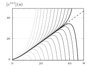
(a) $a=0.5\,(\omega-\lambda)$

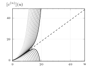
(b) $a=0.8\,(\omega-\lambda)$

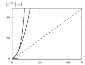
(c) $a=1.0\,(\omega-\lambda)$

Figure 3: (Example C.2) Taylor series for the CVF with exponential service times ($X\sim\textup{Exp}({\omega})$, with $\omega=2\lambda$), and cost function $f(u)=1-e^{-au}$ of exponential type $|a|$ : $c$ (dashed line) and $[{c}^{(n)}]$ for $n=1,\dots,25$. The series only converges if $|a|<|p_{W}|=\omega-\lambda$.

The message of Theorem IV.1 is illustrated by Figure 3, which exposes through an elementary problem the hazards of processing cost functions as Taylor series. See Example C.2 in the appendix for computational details.

System interpretation.

For $n\in\mathbb{N}$, let $\tilde{f}^{(n)}=(\tilde{f}_{0},\dots,\tilde{f}_{n-1})$, with $\tilde{f}_{k}={f^{(k)}(0)}$, and $\tilde{c}^{(n)}=(\tilde{c}^{(n)}_{0},\dots,\tilde{c}^{(n)}_{n-1})$, where $\tilde{c}^{(n)}_{k}$ is defined by (IV.2). Using the matrix inversion lemma, one shows that the Toeplitz, upper triangular matrices

$$\textstyle X^{(n)}=\scalebox{1.0}{$\left(\begin{array}[]{ccccc}x_{1}&x_{2}&x_{3}&\cdots&x_{n}\\ 0&x_{1}&x_{2}&\ldots&x_{n-1}\\ 0&0&x_{1}&\ldots&x_{n-2}\\ \vdots&\vdots&\vdots&\ddots&\vdots\\ 0&0&0&\ldots&x_{1}\end{array}\right)$},\hskip 20.00003ptW^{(n)}=\frac{\lambda}{1-\rho}\scalebox{1.0}{$\left(\begin{array}[]{ccccc}w_{0}&w_{1}&w_{2}&\cdots&w_{n-1}\\ 0&w_{0}&w_{1}&\ldots&w_{n-2}\\ 0&0&w_{0}&\ldots&w_{n-3}\\ \vdots&\vdots&\vdots&\ddots&\vdots\\ 0&0&0&\ldots&w_{0}\end{array}\right)$}.$$

satisfy $W^{(n)}({I^{(n)}}/{\lambda}-X^{(n)})=I^{(n)}$ for all $n$, where $I^{(n)}$ denotes the identity matrix. Besides, (IV.2) rewrites in matrix form as $\tilde{c}^{(n)}=W^{(n)}\tilde{f}^{(n)}$.

As $n\to\infty$, $\{\tilde{c}_{t}\}$ becomes the output (at nonnegative times) of the cross-correlation of $\{\tilde{f}_{t}\}$ with the sequence defined by $\tilde{h}[t]={\lambda}/({1-\rho})w_{t}$ for $t\geq 0$, thus giving us an interpretation for analytic functions of Proposition 2(ii), where $c^{\prime}$ was obtained by cross-correlation of $f(u)$ with $\lambda/(1-\rho)F^{\prime}_{W}({u})$. Similarly, (IV.3b) expresses $c^{\prime}(u)$ as the cross-correlation of the sequence of derivatives of $f$ at $u$ with the sequence $\tilde{h}[t]$.

From our observation follows that the Z-transforms of the sequences satisfy

$$\mathcal{Z}_{\tilde{c}^{(\infty)}}(z)=\mathcal{Z}_{\tilde{h}}({1}/{z})\,\mathcal{Z}_{\tilde{f}^{(\infty)}}(z),$$ (IV.4)

where $\mathcal{Z}_{h}(z)=\sum\nolimits_{k=0}^{\infty}h[k]z^{-k}$ denotes the Z-transform of a sequence $h[t]$. The vector $\tilde{c}^{(\infty)}$ can be recovered from (IV.4) by inverse Z-transform provided that the regions of convergence of $\mathcal{Z}_{\tilde{f}^{(\infty)}}(z)$ and $\mathcal{Z}_{\tilde{h}}({1}/{z})$ intersect on a non-empty circular band—this condition is to be linked to those of Theorem IV.1i.

The conclusions of Theorem IV.1 lead us to consider, in the rest of Section IV, approximations schemes no longer on $\mathbb{R}_{\raisebox{0.5pt}{\tiny$\geq$}0}$, where the growth of the functions $\{u^{n}\}$ as $u\to\infty$ causes divergence, but on finite intervals where the series converge safely.

IV.2 Continuous cost functions

Assume now that the cost function $f$ is continuous, and partition the backlog axis into an interval $(0,\tau)$ where $f$ is approximated precisely (in virtue of the Weierstrass approximation theorem) with respect to the uniform norm $\|f\|=\sup\nolimits_{u\in[0,\tau]}{|f(u)|}$ by a finite sum ${\hat{f}}^{(n)}$ of degree $n$, and its complement $(\tau,\infty)$, where unrefined bounds in $\Xi$ are chosen for $f$. Bounds for the core function can be inferred from the developments of Section III.3.

Notation 4 ($\mathcal{W}$).

Given $\tau>0$ and $\hat{f},\xi\in\Xi$, we denote by $\mathcal{W}(\hat{f};\xi)$ the CVF relative to the cost function $f=\hat{f}\,\mathbf{1}_{(0,\tau)}+\xi\,\mathbf{1}_{(\tau,\infty)}$.

Proposition 3 (Continuous cost).

Consider the server model of Section II.2 with a cost function $f$ meeting Assumption 3, continuous on a nonempty interval $(0,\tau)$, and such that $f\in[f]$, where

$$\begin{array}[]{r}[f]=\{{\hat{f}}^{(n)}+[-{\eta}^{(n)},{\eta}^{(n)}]\}\,\mathbf{1}_{(0,\tau)}+[\xi]\,\mathbf{1}_{(\tau,\infty)},\end{array}$$ (IV.6)

in which ${\hat{f}}^{(n)}$ is a finite sum of degree $n\in\mathbb{N}$, ${\eta}^{(n)}\geq 0$, $[\xi]\equiv[\xi_{-},\xi_{+}]$, and ${\hat{f}}^{(n)},\xi_{-},\xi_{+}$ are real elements of $\Xi$. The core function satisfies

$$\begin{array}[]{l}c\in\left[\mathcal{W}({\hat{f}}^{(n)}-{\eta}^{(n)};\xi_{-}),\mathcal{W}({\hat{f}}^{(n)}+{\eta}^{(n)};\xi_{+})\right],\end{array}$$

where $\mathcal{W}$ (cf. Notation 4) is computed as in Section III.3.

The FPI step can be implemented based on the interval bounds ([AC]) for $[f]$, in place of the actual admission cost (AC’), provided that the parameters $\tau$ and $n$ chosen for the servers allow for it. Otherwise, the parameter values should be refined (by increasing $\tau$ and $n$) until decision (D) can be made.

A pseudocode for the resulting procedure is given in Algorithm 8, where the cost function $f_{i}$ of each server $i$ is supplied with a continuum of bounding interval functions $[\xi_{i}]$ such that, for every $\tau>0$, $f_{i}(u_{i})\in[\xi_{i}(\tau)](u_{i})$ if $u_{i}>\tau$. Algorithm 8 infers the FPI decision $\hat{\pi}{(u,x)}$ at any state $(u,x)$ by gradually decreasing the error tolerance $\epsilon_{t}$ of the admission cost bounds at each server, computed by (IV.6). To guarantee the error margin $\epsilon_{t}$ at a server $i$, the parameter $\tau_{i}$ is first taken large enough for the approximation error in the $u>\tau_{i}$ window to be less than ${\epsilon_{t}}/{2}$ (line 1), then the sum ${\hat{f}}^{(n)}$ is given enough terms for the approximation error in the $0<u<\tau_{i}$ window to be less than ${\epsilon_{t}}/{2}$ (line 1), so that the overall precision $\epsilon_{t}$ is secured for the bounds $[\hat{f}_{i}]$ (line 1). All servers with exceeding admission costs will be ignored (line 1) for the rest of the procedure, which resumes with a smaller margin $\epsilon_{t+1}$.

List of algorithmenvs 1 FPI with interval value functions

 

Data: $\{(\lambda_{1},f_{1},[\xi_{1}]),\dots,(\lambda_{k},f_{k},[\xi_{k}])\}$, $\{\epsilon_{t}\}$ with $\epsilon_{t}\downarrow 0$

Input : $(u,x)\in\mathbb{R}_{\raisebox{0.5pt}{\tiny$\geq$}0}^{k}\times\mathbb{R}_{\raisebox{0.5pt}{\tiny$\geq$}0}^{k}$

Output : $\pi\subset\{1,\dots,k\}$

Initialization: $t\leftarrow 0$, $\pi\leftarrow\{1,\dots,k\}$, $[\hat{f}_{i}]\leftarrow(-\infty,\infty)$ for all $i\in\pi$

  ;

While  $t\leq t_{\textup{max}}$ and $|\pi|>1$ do

      For $i\in\pi$ do

1           $\tau_{i}\leftarrow\arg\inf\nolimits_{\tau\geq 0}\big{\{}\big{|}[\mathcal{A}_{i}]\left([\xi_{i}(\tau)]\,\mathbf{1}_{(\tau,\infty)};u,x\right)\big{|}\leq{\epsilon_{t}}/{2}\big{\}}$ ;

2           $n_{i}\leftarrow\arg\min\nolimits_{n}\big{\{}\big{|}\mathcal{A}_{i}\left(\mathbf{1}_{(0,\tau_{i})};u,x\right)\big{|}\leq{\epsilon_{t}}/({4{\eta}^{\scalebox{0.8}{\tiny$(n)$}}})\big{\}}$ ;

3           $[\hat{f}_{i}]\leftarrow\big{\{}{\hat{f}_{i}}^{\scalebox{0.8}{\tiny$(n_{i})$}}+[-{\eta}^{\scalebox{0.8}{\tiny$(n_{i})$}},{\eta}^{\scalebox{0.8}{\tiny$(n_{i})$}}]\big{\}}\,\mathbf{1}_{(0,\tau_{i})}+[\xi_{i}(\tau_{i})]\,\mathbf{1}_{(\tau_{i},\infty)}$;

4          

           For $i\in\pi$ do

5                If $\exists j\in\pi{\setminus}\{i\}$ such that $[\mathcal{A}_{i}]\left([\hat{f}_{i}];u,x\right)>[\mathcal{A}_{j}]\left([\hat{f}_{j}];u,x\right)$ then $\pi\leftarrow\pi{\setminus}\{i\}$;

6               

7               

 

In Sections IV.2.1 and IV.2.3 we discuss the methods for deriving the finite sum $[{\hat{f}}^{(n)}]$ when the cost function $f$ is continuous on any support $[0,\tau]$.

IV.2.1 Bernstein polynomials

The function $f$ can be approximated on $[0,\tau]$ by the Bernstein polynomial bernstein12

$$b^{(n)}{(u)}=\sum\nolimits_{l=0}^{n}\Big{(}\begin{array}[]{c}{n}\\ {l}\end{array}\Big{)}\,\Big{(}\frac{u}{\tau}\Big{)}^{l}\Big{(}1-\frac{u}{\tau}\Big{)}^{n-l}f\left({l\tau}/{n}\right), \forall u\in[0,\tau].\hskip 10.00002pt$$ (IV.9)

Notice that (IV.9) rewrites as $b^{(n)}{(u)}=\mathbb{E}[f({K\tau}/{n})]$, where the random variable $K\sim\textup{B}(n,u/\tau)$ is distributed according to the binomial distribution with $n$ trials and success probability $u/\tau$. The quantity $K/n$ has mean $u/\tau$ and variance $({u}/{\tau})(1-{u}/{\tau})/n\leq 1/(4n)$, which vanishes uniformly on $[0,\tau]$. It follows from continuity arguments that $\mathbb{E}[f({K\tau}/{n})]$ converges uniformly towards $f(u)$ on that interval, (koralov07, , proof of Theorem 2.7). So does (IV.9), with rate

$$\|f-b^{(n)}\|\leq({3}/{2})\,\omega\big{(}f;[0,\tau];{\tau}/{\sqrt{n}}\big{)},$$ (IV.10)

(rivlin69, , Theorem 1.2), where

$$\textstyle\omega(f;[0,\tau];\delta)=\sup\{|f(u_{1})-f(u_{2})|:u_{1},u_{2}\in[0,\tau],|u_{1}-u_{2}|\leq\delta\}$$

defines the modulus of continuity of $f$ on the interval $[0,\tau]$, (jackson41, , §21). To conform with (IV.6), we rewrite (IV.9) as

$$b^{(n)}{(u)}=\sum\nolimits_{k=0}^{n}\beta_{n,k}u^{k}, \forall u\in[0,\tau],$$ (IV.11)

where $\textstyle\beta_{n,k}=(-\tau)^{-k}\big{(}{}^{n}_{k}\big{)}\sum\nolimits_{l=0}^{k}\big{(}{}^{k}_{l}\big{)}(-1)^{l}f({l\tau}/{n})$, for $k=0\dots,n$.

From (IV.10) and (IV.11), we infer bounds for the value function.

Corollary 1 (Bernstein polynomials).

Proposition 3 holds for ${\hat{f}}^{(n)}\equiv b^{(n)}$ defined by (IV.11) with the uniform error bound ${\eta}^{(n)}={3}/{2}\,\omega(f;[0,\tau];{\tau}/{\sqrt{n}})$.

IV.2.2 Approximation by trigonometric sums

A better convergence rate for ${\hat{f}}^{(n)}$ can be obtained using trigonometric sums; we refer to (rivlin69, , §1.1) for details on this topic. Consider the continuous, $2\tau$-periodic function $\check{f}:\mathbb{R}\mapsto\mathbb{R}$ defined on $[-\tau,\tau]$ by $\check{f}(u)=f(|u|)$. The Weierstrass approximation theorem (see, e.g., (korovkin60, , Weierstrass first theorem), (rivlin69, , Theorem 1.1), (koralov07, , Theorem 2.7)) claims that $\check{f}$ can be approximated by a trigonometric sum with arbitrary precision with respect to the uniform norm $\|f\|=\sup\nolimits_{u\in[-\tau,\tau]}|f(u)|$. This implies that for any $\epsilon>0$ one can find $n<\infty$ and a trigonometric sum $t^{(n)}$ such that ${\eta}^{(n)}=\|\check{f}(u)-t^{(n)}{(u)}\|<\epsilon$. It then follows that $f\in[f]=t^{(n)}+[-{\eta}^{(n)},{\eta}^{(n)}]$. Such a trigonometric sum is given by the partial Fourier series, which for the real, even function $\check{f}$ reduces to

$$t^{(n)}{(u)}=\check{\alpha}_{0}+2\sum\nolimits_{k=1}^{n}\check{\alpha}_{k}\,\cos({k\pi u}/{\tau}),$$ (IV.13)

where

$$\check{\alpha}_{k}=\frac{1}{\tau}\int\nolimits_{0}^{{\tau}}f({u})\cos({k\pi u}/{\tau})\,du, (k\in\mathbb{N}).$$ (IV.14)

are the Fourier coefficients. With the modulus of continuity of $\check{f}$ defined by

$$\omega(\check{f};\delta)=\sup\{|\check{f}(u_{1})-\check{f}(u_{2})|:u_{1},u_{2}\in\mathbb{R},|u_{1}-u_{2}|\leq\delta\},$$ (IV.15)

the Fourier series (IV.13) converges towards the periodic function $\check{f}$ with rate $O({\eta}^{(n)})=\log(n)\,\omega(\check{f};\tau/(n\pi))$, (jackson41, , §21). Faster convergence can be obtained by slightly modifying the Fourier coefficients in (IV.13). For this, consider

$$\check{t}^{(n)}{(u)}=\varrho_{n,0}\,\check{\alpha}_{0}+2\sum\nolimits_{k=0}^{n}\varrho_{n,k}\,\check{\alpha}_{k}\,\cos({k\pi u}/{\tau}),$$ (IV.16)

where $\varrho_{n,0},\dots,\varrho_{n,n}\in\mathbb{R}$. The choice of parameters proposed in (korovkin60, , §3),

$$\textstyle\varrho_{n,0}{\,=\,}1,\ \varrho_{n,1}{\,=\,}\cos(\frac{\pi}{n+2}),\ \varrho_{n,k}{\,=\,}\frac{\sum\nolimits_{q=0}^{n-k}\sin\left(\frac{q+1}{n+2}\pi\right)\sin\left(\frac{q+k+1}{n+2}\pi\right)}{\sum\nolimits_{q=0}^{n}\sin^{2}\left(\frac{q+1}{n+2}\pi\right)}\textup{ for }k=2,\dots,n,$$ (IV.17)

lends (IV.16) the convergence rate

$$\begin{array}[]{l}{\eta}^{(n)}\leq 6\,\omega\left(\check{f};\frac{\tau}{\pi n}\right),\end{array}$$ (IV.18)

(see (korovkin60, , first Jackson Theorem), or (rivlin69, , Theorem 1.3)). Since $\check{t}^{(n)}\in\Xi$ and by construction $\omega(\check{f};\cdot)\equiv\omega(f;[0,\tau];\cdot)$, $\check{t}^{(n)}$ is a candidate finite sum for Proposition 3 and (IV.18) gives us bounds for the value function.

Corollary 2 (Trigonometric sums).

Proposition 3 holds for ${\hat{f}}^{(n)}\equiv b^{(n)}$ defined by (IV.11) with the uniform error bound ${\eta}^{(n)}={3}/{2}\,\omega(f;[0,\tau];{\tau}/{\sqrt{n}})$.

In particular, if for some $\alpha\in(0,1]$ the cost function satisfies the $\alpha$-Höldern condition $|f(u_{1})-f(u_{2})|\leq h|u_{1}-u_{2}|^{\alpha}$ for all $u_{1},u_{2}\in[0,\tau]$, then $\omega(f;[0,\tau];\delta)\leq h\delta^{\alpha}$, and (IV.13) converges uniformly towards $f$ on $[0,\tau]$ with ${\eta}^{(n)}=O(({\tau}/n)^{\alpha})$. If $f$ is Lipschitz continuous on $[0,\tau]$ with modulus $L$, then ${\eta}^{(n)}<2L{\tau}/n$.

IV.2.3 Near-optimal polynomial approximation

Alternatively, the convergence rate of Corollary 3 can be obtained using polynomials. Set $\tilde{f}:\mathbb{R}\mapsto\mathbb{R}$ to be the continuous, $2\pi$-periodic function defined by $\tilde{f}(\theta)=f(\tilde{u}(\theta))$, where $\tilde{u}(\theta)=({\tau}/{2})\,(1+\cos(\theta))$. It follows from the $({\tau}/{2})$-Lipschitz continuity of $\tilde{u}$ and the definition (IV.15) of the modulus of continuity, that $\omega(\tilde{f};\delta)\leq\omega(f;[0,\tau];{\tau\delta}/{2})$ for $\delta>0$. Proceeding as in (IV.16), we consider the trigonometric sum for $\tilde{f}$ given by the modified Fourier series

$$\tilde{t}^{(n)}{(\theta)}=\sum\nolimits_{k=0}^{n}\varrho_{n,k}\beta_{k}\cos(k\theta), \forall\theta\in\mathbb{R},$$ (IV.19)

where $\beta_{0}=\tilde{\alpha}_{0}$, $\beta_{k}=2\tilde{\alpha}_{k}$ if $k\geq 1$, and $\tilde{\alpha}_{k}=({1}/{\pi})\int\nolimits_{0}^{{\pi}}\tilde{f}(\theta)\cos(k\theta)\,d\theta$ for $k\in\mathbb{N}$. Defining $\varrho_{n,k}$ as in (IV.17), yields the uniform convergence rate

$$\|f-\tilde{t}^{(n)}\|=\overset{\text{\tiny{\eqref{mirrorjacksontrigonometric}}}}{\leq}6\,\omega\left(\tilde{f};1/n\right)\leq 6\,\omega\left(f;[0,\tau];{\tau}/({2n})\right).$$ (IV.20)

It remains to rewrite (IV.19) as a polynomial in $u$ by returning to the backlog domain. For this, we develop $\cos(k\theta)=\Re\left((\cos(\theta)+i\sin(\theta))^{k}\right)$ and find $\cos(k\theta)=p_{k}(\cos(\theta))$, where the polynomial $p_{k}(x)$, characterized by its $k$ real roots located in $(-1,1)$, is defined by

$$p_{k}(x)=\left\{\begin{array}[]{ll}\sum\nolimits_{q=0}^{{k}/{2}}\nu(k,q)x^{2q},&\hskip 10.00002pt\textup{if~{}$k$ is even}\\ \sum\nolimits_{q=0}^{({k-1})/{2}}\nu(k,q)x^{2q+1},&\hskip 10.00002pt\textup{if~{}$k$ is odd}\end{array}\right\},$$ (IV.21)

where $\nu(0,0)=1$, and

$$\textstyle\nu(k,q)=(-1)^{\lfloor\frac{k}{2}\rfloor-q}\sum\nolimits_{t=0}^{q}\left({}^{\ \ \ \ k}_{2(\lfloor\frac{k}{2}\rfloor-t)}\right)\left({}^{\lfloor\frac{k}{2}\rfloor-t}_{\lfloor\frac{k}{2}\rfloor-q}\right),\hskip 10.00002pt(q=0\dots,\left\lfloor\frac{k}{2}\right\rfloor,\,k\in\mathbb{N}_{>0}).$$

Since $\tilde{f}(\theta)=f(\tau(1+\cos(\theta))/2)$, a polynomial approximation of $f$ on $[0,\tau]$ is obtained by setting $\cos(k\theta)=p_{k}(2u/\tau-1)$ in (IV.19), and we find, after straightforward computations,

$$\hat{t}^{(n)}{(u)}=\sum\nolimits_{k=0}^{n}\gamma(n,k)u^{k}, \forall u\in[0,\tau],$$ (IV.22)

where we define

$$\gamma(n,k)=({2}/{\tau})^{k}\,\sum\nolimits_{t=0}^{n-k}\Big{(}\begin{array}[]{c}{t+k}\\ {\ k}\end{array}\Big{)}\,(-1)^{t}\,\bar{\gamma}(n,t+k), (k=0\dots,n).$$ (IV.25)

and $\bar{\gamma}(n,t)=\sum\nolimits_{k\in\bar{\sigma}(n,t)}\varrho_{n,k}\,\beta_{k}\,\nu(k,\lfloor t/2\rfloor)$ for $t=0,\dots,n$, in which $\bar{\sigma}(n,t)=\{t,t+2,t+4,\dots,n\}$ if $n-t$ is even, and $\bar{\sigma}(n,t)=\{t,t+2,t+4,\dots,n-1\}$ otherwise ($0\leq t\leq n$). As for the Fourier coefficients of $\tilde{f}$, they reduce to

$$\tilde{\alpha}_{k}=\frac{1}{\pi}\int\nolimits_{0}^{{\pi}}f(\tilde{u}(\theta))\cos(k\theta)\,d\theta\overset{\text{\tiny{\eqref{polycostnx}}}}{=}\frac{1}{\pi}\int\nolimits_{0}^{\tau}f(u)\frac{p_{k}(\frac{2u}{\tau}-1)}{\sqrt{u(\tau-u)}}\,du,$$ (IV.26)

where we have used the change of variable $u=\tilde{u}(\theta)$. For many cost functions, the coefficients $\{\tilde{\alpha}_{k}\}$ can be derived exactly. See Lemma D.1 for expressions of these coefficients in the case when $f$ is given as a quotient of polynomials.

From (IV.20), we infer the following bounds for the value function.

Corollary 3 (Near-optimal polynomials).

Proposition 3 holds for ${\hat{f}}^{(n)}\equiv\hat{t}^{(n)}$ defined by (IV.22) with uniform error bound ${\eta}^{(n)}=6\,\omega(f;[0,\tau];{\tau}/({2n}))$.

Without further assumptions on $f$, the convergence rate $O(\omega(f;[0,\tau];{\tau}/({2n})))$ guaranteed by (IV.22) is non-improvable. The performance of $\check{t}^{(n)}$ and $\hat{t}^{(n)}$ in Corollaries 2 and 3 are then really close, and the choice of either approach (Section IV.2.2 or IV.2.3), mostly dependent on the computability of the Fourier coefficients (IV.14) or (IV.26), respectively, is left to the appreciation of the reader. The second approach nevertheless prevails in the event the cost function has a $k$th derivative $f^{(k)}$ on $[0,\tau]$. Then, the convergence rate in Corollary 3 can be lowered to $O(n^{-k}\omega(f^{(k)};[0,\tau];{\tau}/[{2(n-k)}]))$ by using the derivatives as the targets of approximation, (rivlin69, , Theorem 1.5). This distinguishing property of approach IV.2.3 stems from the fact that $\tilde{f}(\theta)$ retains the smoothness of the cost function, whereas $\check{f}(u)$ shows irregularities at $u=(2k+1)\tau$. We refer to (rivlin69, , §1.1) and references therein for further considerations on the optimality of (IV.20) as a convergence rate for polynomial approximations.

Case study: quotient cost function.

Let $f(u)={u^{2}}/({a^{2}+u^{2}})$, where $a>0$ is a positive parameter. The Fourier coefficients (IV.26) for $f$ are given by Lemma D.1 with $l({k})\equiv k$. After computation of the residues at the complex conjugate poles $ia$ and $-ia$, (D.9) reduces to

$$\begin{array}[]{ll}\tilde{\alpha}_{k}=\sqrt{\pi}\sum\nolimits_{q=0}^{k}\frac{\zeta_{-q}\,(-\tau)^{q}}{{q}!\Upgamma\left(\frac{1}{2}-q\right)}-\frac{\sqrt{a}}{\sqrt[4]{a^{2}+\tau^{2}}}\sum\nolimits_{q=0}^{\lfloor\frac{k}{2}\rfloor}\kappa(k,\tau,q)\,\nu(k,q),&\hskip 10.00002pt(k\in\mathbb{N}_{\geq 0}),\end{array}$$

where $\{\zeta_{-q}\}_{q=0}^{k}$ are the first $k+1$ coefficients (i.e., those associated with nonnegative powers) of the Laurent series at $+\infty$ of $f(u)\,p_{k}({2u}/{\tau}-1)$, equal in this example to

$$\zeta_{-q}\overset{\text{\tiny{\eqref{laurentcoef}}}}{=}\left\{\begin{array}[]{ll}(\frac{-2}{\tau})^{q}\sum\nolimits_{l=\lceil\frac{q}{2}\rceil}^{\frac{k}{2}}\big{[}\sum\nolimits_{t=0}^{l-\lceil\frac{q}{2}\rceil}\big{(}{}^{\,2l}_{q+2t}\big{)}\big{(}\frac{-4a^{2}}{\tau^{2}}\big{)}^{t}\big{]}\nu(k,l),&\textup{if~{}$k$ even }\\ -(\frac{-2}{\tau})^{q}\sum\nolimits_{l=\lceil\frac{q-1}{2}\rceil}^{\frac{k-1}{2}}\big{[}\sum\nolimits_{t=0}^{l-\lceil\frac{q-1}{2}\rceil}\big{(}{}^{2l+1}_{q+2t}\big{)}\big{(}\frac{-4a^{2}}{\tau^{2}}\big{)}^{t}\big{]}\nu(k,l),\hskip 10.00002pt&\textup{if $k$ odd}\end{array}\right\}$$

where we used $\{{\kappa(k,\tau,q)}\}_{q=0}^{\lfloor\frac{k}{2}\rfloor}$, defined for $k$ even and $q=0,\dots,\frac{k}{2}$ by

$$\textstyle\kappa(k,\tau,q)=\cos\big{(}\frac{\theta(a,\tau)}{2}\big{)}\sum\nolimits_{t=0}^{q}\big{(}{}^{2q}_{2t}\big{)}\big{(}\frac{-4a^{2}}{\tau^{2}}\big{)}^{t}-\frac{2a}{\tau}\sin\big{(}\frac{\theta(a,\tau)}{2}\big{)}\sum\nolimits_{t=0}^{q-1}\big{(}{}^{2q}_{2t+1}\big{)}\big{(}\frac{-4a^{2}}{\tau^{2}}\big{)}^{t},$$

and for $k$ odd and $q=0,\dots,\frac{k-1}{2}$ by

$$\textstyle\kappa(k,\tau,q){=}{-}\cos\big{(}\!\frac{\theta(a,\tau)}{2}\!\big{)}\!\sum\nolimits_{t=0}^{q}\!\big{(}{}^{{2q{+}1}}_{\ \,2t}\big{)}\big{(}\!\frac{{-}4a^{2}}{\tau^{2}}\!\big{)}^{t}{+}{\frac{2a}{\tau}}\sin\big{(}\!\frac{\theta(a,\tau)}{2}\!\big{)}\!\sum\nolimits_{t=0}^{q}\!\big{(}{}^{2q{+}1}_{2t{+}1}\big{)}\big{(}\!\frac{-4a^{2}}{\tau^{2}}\!\big{)}^{t},$$

in which $\theta(a,\tau)=\tan^{-1}(\frac{\tau}{a})$.

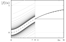
(a) Cost function intervals.

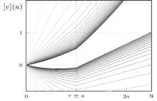
(b) Value function intervals (exponentially distributed service times; $\omega=2$, $\lambda=1$).

Figure 4: Intervals for $f(u)={u^{2}}/({a^{2}+u^{2}})$ as per Corollary 3 ($n=1,\dots,20$).

The continuity modulus of $f$ on $[\delta/2,\tau-\delta/2]$ is given, for $\delta\in[0,{\tau}/{2}]$, by $\omega(f;[0,\tau];\delta)=f(u^{\star}(\delta)+\delta/2)-f(u^{\star}(\delta)-\delta/2)$, where

$$\textstyle u^{\star}(\delta)=\min\Big{\{}\sqrt{\frac{(\frac{\delta}{2})^{2}-a^{2}+2\sqrt{a^{4}+a^{2}(\frac{\delta}{2})^{2}+(\frac{\delta}{2})^{4}}}{3}},\tau-\frac{\delta}{2}\Big{\}}$$

satisfies ${\delta}/{2}<u^{\star}(\delta)\leq\tau-{\delta}/{2}$. The cost function $f$ is approximated by (IV.6), with ${\hat{f}}^{(n)}\equiv\hat{t}^{(n)}$ given by (IV.22) and $[\xi]$ set to

$$\begin{array}[]{ll}[\xi](u)=\big{[}f(\tau),-\left(1-f(\tau)\right)\operatorname{exp}\big{\{}{-\big{(}\frac{f^{\prime}(\tau)}{1-f(\tau)}\big{)}(u-\tau)}\big{\}}\big{]},&\hskip 10.00002ptu\geq\tau,\end{array}$$

in which $f^{\prime}(\tau)=2a^{2}\tau(a^{2}+\tau^{2})^{-2}$. The intervals produced by Corollary 3 for $f$, and for its value function in the presence of jobs with exponentially-distributed service times are displayed in Figure 4, for fixed $\tau$ and $n=1,\dots,20$. The value function intervals shown in Figure 4(b) followed from (IV.22) and the developments of Examples C.3 and C.4. The interval gaps can be arbitrarily reduced by increasing both $n$ and $\tau$, as in Algorithm 8.

Consider a system of two parallel servers $1$ and $2$, with server $1$ twice faster than $2$. Feed the system a sequence of jobs with arrival rate $\lambda=3/2$ and service times exponentially distributed with parameters $(\omega_{1},\omega_{2})=(2,1)$. Assume that the workload is initially balanced between the two servers, i.e., $(\lambda_{1},\lambda_{2})=(1,1/2)$, and let $f(u)={u^{2}}/({a^{2}+u^{2}})$.

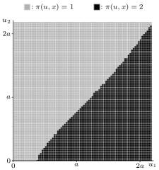
(a) $\pi(u,x)$ for $x=(1,2)$.

(b) Minimum order $n^{\star}(u,x)$ needed in (IV.22) for decision, $x=(1,2)$.

Figure 5: One-step policy improvement for a two-server system $(1,2)$ with arrival rates $(\lambda_{1},\lambda_{2})=(1,1/2)$, exponentially distributed service times with parameters $(\omega_{1},\omega_{2})=(2,1)$, and cost function $f(u)={u^{2}}/({a^{2}+u^{2}})$.

Figure 5(a) depicts, for a particular job with service times $(x_{1},x_{2})=(1,2)$ and for various backlog $u=(u_{1},u_{2})$, the FPI policy $\pi(u,x)$ issued by Algorithm 8. The quantity $n^{\star}(u,x)$ displayed in Figure 5(b) is the minimum order $n$ required in (IV.22) for dispatching at $(u,x)$. This quantity was estimated by reporting the minimum order that allowed for dispatching for a coarse grid of values of the parameter $\tau$. It can be seen that $n^{\star}(u,x)$ grows with the distance to the origin $u=(0,0)$, and increases abruptly near the frontiers of the dispatching policy $\pi$. The relatively high orders rendered by Figure 5(b) are due to the conservativeness of the uniform error bound ${\eta}^{(n)}\equiv 6\,\omega(f;[0,\tau];{\tau}/({2n}))$ for this particular choice of the cost function (cf. Figure 4(a)). In practice, more accurate estimates of the error bound would contribute to reducing the estimation orders. More generally, building the function approximations from the $k$ first derivatives of $f$, as previously suggested, will significantly accelerate convergence.

V Discussion

Integral transformations of the Poisson equation $g=Pg+f$ have the quality of simplifying the analysis, as they provide a principled framework for the systematic derivation of solutions. Although it is known that the candidate functions for closed-form solutions form a dense set where any $f$ can be approximated with arbitrary precision, one should be cautious that a convergent series for $f$ does not always produce a convergent series for $g$; Taylor series of $f$, in particular, are subject to tail effects and most likely to diverge after $\mu_{W}$-integration with respect to the stationary probability measure of the waiting times.

In the context of first-policy improvement, such tail effects can be avoided by considering approximations of $f$ on finite supports—preferably trigonometric sums, which for Lipschitz-continuous $f$ achieve the convergence rate $O(\tau/n)$ in the number $n$ of approximation terms, improvable to $O({\tau}/[(n-k)n^{k}])$ if $f$ is $k$-times continuously differentiable—, while using tractable bounds for the larger backlog values. The availability of closed forms for bounding intervals of this type with a diversity of service time distribution models gives the green light to a systematized implementation of the FPI step.

We believe that the techniques developed in this study, combined with well-chosen supervised learning methods, make it possible, in large multiple-server systems, to devise efficient online algorithms for learning FPI policies gradually, as the incoming jobs are dispatched and the (possibly high-dimensional) state space is visited. The design and assessement of FPI dispatching policies in such systems is left to future work.

Appendix A Characterization of the value function

Before showing Propositions 1-2, and Theorem III.1, we characterize $W^{\ast}$ in the complex plane.

Proposition A.1 (Analycity of $W^{\ast}$ and pole location).

Under Assumption 1:

1. The dominant singularity $p_{W}$ of $W^{\ast}$ (i.e., that with largest real value) is a pole with degree $1$ lying on the negative real axis $\mathbb{R}_{<0}$. The dominant singularity $p_{X}$ of $X^{\ast}$ is real, negative (possibly infinite) and satisfies $p_{X}<p_{W}$. $X^{\ast}$ is analytic on $\{s\in\mathbb{C}\,|\,\Re\left(s\right)>p_{W}\}$.

2. $W^{\ast}$ is analytic on $\{s\in\mathbb{C}_{0}\,|\,\Re\left(s\right)>p_{W}\}$, where $\lim\nolimits_{s\to\infty}|W^{\ast}(s)|\leq 1$.

3. One can find $\epsilon>0$ such that $W^{\ast}$ is analytic on $\{s\in\mathbb{C}_{0}\setminus\{p_{W}\}\,|\,\Re(s)>p_{W}-\epsilon\}$.

4. $W^{\ast}$ is analytic in a neighborhood of $0$, where it rewrites as the series

   $$\begin{array}[]{ll}W^{\ast}(s)=\sum\nolimits_{k=0}^{\infty}w_{k}\,(-s)^{k},&\forall s\in\{\sigma\in\mathbb{C}_{0}:|\sigma-a|<|p_{W}|\},\end{array}$$ (A.1)

   in which the coefficients $\{w_{k}\}$ are given by (III.3) in Table 1, and satisfy $w_{k}=\mathbb{E}[W^{k}]/{k}!$, for $k\in\mathbb{N}$. The series $\{w_{k}\}$ is asymptotically geometric with asymptotic rate $|p_{W}|^{-1}$.

5. At any point $a\in\mathbb{C}_{0}$ where $W^{\ast}$ is analytic, $W^{\ast}$ rewrites as the series

   $$\begin{array}[]{ll}W^{\ast}(s)=\sum\nolimits_{k=0}^{\infty}w_{{a}:{k}}(a-s)^{k},&\forall s\in\{\sigma\in\mathbb{C}:|\sigma-a|<r_{a}\},\end{array}$$ (A.2)

   where $r_{a}$ denotes the distance from $a$ to the closest singularity of $W^{\ast}$. The coefficients $\{w_{{a}:{k}}\}$ are given by (III.4) in Table 1.

Next, we derive the identities of Section III.1 for the value function.

Proposition 1.

Start the queue at state $u$. The quantity $V(u,t)$ appearing in (VF) rewrites, for any $T\geq 0$ and for $t$ large enough, as $V(u,t)=V(u,T)+V(U({T}),t-T)$, where $U({T})$ denotes the backlog observed after time $T$. It follows from the Markov property of the system and from the the definition VF of the value function that

$$v(u)=\mathbb{E}[V(u,T)-\lambda\bar{f}T]+\mathbb{E}[v(U({T}))].$$ (A.3)

Now, consider the function

$$\textstyle g({u,x})=\lim\nolimits_{N\to\infty}\{\sum_{n=1}^{N}\mathbb{E}\left[f(U_{n})-\bar{f}\right]\,|\,(U_{1},X_{1})=(u,x)\}+\bar{f},\hskip 10.00002pt\forall u,x\in\mathbb{R}_{\raisebox{0.5pt}{\tiny$\geq$}0},$$ (A.4)

which can be verified to satisfy Equation (PE) by application of the Markov property to the MDP. The function $g$ defined by (A.4) can be seen as a discrete-time counterpart of the value function (VF), which follows from (A.4) by using the convention $(U_{0},X_{0})=(u,0)$ and setting $v(u)\equiv Pg({u,0})-\bar{f}$ or, equivalently, from (A.3) by defining $T$ as the arrival time of the first job so that $\mathbb{E}[V(u,T)-\lambda\bar{f}T]=-\bar{f}$ and $\mathbb{E}[v(U({T}))]\equiv Pg({u,0})$. $\square$ $\square$

Theorem III.1.

A simple calculation reveals that $\Updelta(u)=0$ if $u<0$, and $\textstyle\Updelta(u)=(P-\widehat{P})g({u,0})=\kappa e^{-\lambda u}$, for $u\geq 0$, with $\kappa$ satisfying by

$$\textstyle\kappa=\mathbb{E}\big{[}g({0,X_{0}})-\lambda\int_{-\infty}^{0}g({u,X})\,e^{\lambda u}\,du\big{]}.$$ (A.5)

We characterize the extended value function $\widehat{v}:u\in\mathbb{R}\mapsto\widehat{v}(u)=g({u,0})-f(u)$ associated with some $g$ solution of (PE’). Note that, by construction, $\widehat{v}$ coincides with the value function on $\mathbb{R}_{\raisebox{0.5pt}{\tiny$\geq$}0}$, i.e., $\widehat{v}(u)\equiv v(u)$ if $u\geq 0$. Once $\widehat{v}$ is known, it will be possible to recover $g$ using

$$g({u,x})=g({u+x,0})-f(u+x)+f(u)=\widehat{v}(u+x)+f(u).$$ (A.6)

Consider $s$ in the region of absolute convergence of $\mathcal{B}_{\widehat{v}}$, where the orders of integration in our developments may be permuted. The two-sided Laplace transform of $\widehat{v}$ is given by

$$\begin{array}[]{rcl}\mathcal{B}_{\widehat{v}}(s)&=&\int_{-\infty}^{+\infty}\widehat{v}(u)\,e^{-su}\,du\\ &=&\int_{-\infty}^{+\infty}[g({u,0})-f(u)]\,e^{-su}\,du\\ &\overset{\text{\tiny{\eqref{rMG1Poisson}}}}{=}&\int_{-\infty}^{+\infty}[\widehat{P}g({u,0})+\Updelta(u)-\bar{f}\,\mathbf{1}_{[0,+\infty)}(u)]\,e^{-su}\,du\\ &=&\int_{-\infty}^{+\infty}e^{-su}\,du\int g({t,x})\widehat{P}({u,0},d(t,x))+\int_{0}^{+\infty}\kappa e^{-(s+\lambda)u}\,du-\frac{\bar{f}}{s}\\ &\overset{\text{\tiny{\eqref{UMDPkernel}}}}{=}&\lambda\mathbb{E}\big{[}\int_{-\infty}^{+\infty}e^{-su}\,du\,\int_{-\infty}^{u}g({t,X})e^{-\lambda(u-t)}\,dt\big{]}-\frac{\bar{f}}{s}+\frac{\kappa}{s+\lambda}\\ &=&\lambda\mathbb{E}\big{[}\int_{-\infty}^{+\infty}g({t,X})\,e^{\lambda t}\,dt\int_{t}^{+\infty}e^{-(s+\lambda)u}\,du\big{]}-\frac{\bar{f}}{s}+\frac{\kappa}{s+\lambda}\\ &\overset{\text{\tiny{\eqref{altgenericxidentity}}}}{=}&\frac{\lambda}{s+\lambda}\big{\{}\mathbb{E}\big{[}\int_{-\infty}^{+\infty}\widehat{v}(t+X)\,e^{-st}\,dt\big{]}+\int_{0}^{+\infty}f(t)\,e^{-st}\,dt\big{\}}-\frac{\bar{f}}{s}+\frac{\kappa}{s+\lambda}\\ &=&\frac{\lambda}{s+\lambda}\big{\{}X^{\ast}(-s)\,\mathcal{B}_{\widehat{v}}(s)+\mathcal{L}_{f}(s)-\frac{\bar{f}}{s}+\frac{\kappa-\bar{f}}{\lambda}\big{\}}.\end{array}$$

Solving the above equation for $\mathcal{B}_{\widehat{v}}(s)$ and using $W^{\ast}(-s)=1+{\lambda\mathbb{E}[X^{2}]}/[{2(1-\rho)}]s+o(s)$ yields, after computations,

$$\begin{array}[]{rcl}\mathcal{B}_{\widehat{v}}(s)&\overset{\text{\tiny{\eqref{PKformula}}}}{=}&\frac{\lambda W^{\ast}(-s)}{(1-\rho)s}\left[\mathcal{L}_{f}(s)-\frac{\bar{f}}{s}+\frac{\kappa-\bar{f}}{\lambda}\right]\\ &=&\frac{\lambda}{(1-\rho)s}W^{\ast}(-s)\mathcal{L}_{f}(s)-\frac{\lambda\bar{f}}{(1-\rho)s^{2}}+\frac{\varepsilon}{s}+\frac{h(s)}{s},\end{array}$$ (A.7)

where $h(s)$ has no singularities on $\{s\in\mathbb{C}\,|\,\Re\left(s\right)<-p_{W}\}$, and $\varepsilon$ is given by

$$\varepsilon={\kappa}/{(1-\rho)}-{\hat{X}^{\ast}_{2}(\lambda)\bar{f}}/{(1-\rho)^{2}},$$ (A.8)

with $\hat{X}^{\ast}_{2}(\lambda):=1-\lambda\mathbb{E}[X]+\lambda^{2}\mathbb{E}[X^{2}]/2$. Since $\widehat{v}$ is expected to be asymptotically flat for $u\to-\infty$, the $-{\lambda\bar{f}}/[{(1-\rho)s^{2}}]$ term in (A.7) is necessarily due to a term $-{\lambda\bar{f}}/({1-\rho})\,u$ on $\mathbb{R}_{\raisebox{0.5pt}{\tiny$\geq$}0}$ in the backlog domain. By inverse transformation of (A.7), we find

$$\textstyle\widehat{v}(u) \textstyle=\widehat{v}(0)+c(u)-\frac{\lambda\bar{f}}{1-\rho}u\,\mathbf{1}_{[0,+\infty)}(u)+r(u)\,\mathbf{1}_{(-\infty,0)}(u), \forall u\in\mathbb{R}, \widehat{\text{S}}$$ ()

where $r$ satisfies $\mathcal{L}_{r(-\cdot)}(s)=-[{h(-s)+\varepsilon}]/{s}$. The general form for $g$ follows from (A.6), ($\widehat{\text{S}}$) and $\widehat{v}(u)\equiv v(u)$ on $\mathbb{R}_{\raisebox{0.5pt}{\tiny$\geq$}0}$. The non-empty ROC of $\mathcal{B}_{\partial_{+}\widehat{v}}$ is the consequence of Assumption 3.

It remains to show that the function $r$ is identical for all solutions or, equivalently, that the quantity $\kappa$ in (A.5) is the same for all $g$. To see this, consider a solution $g_{1}$ of (PE’) with associated value function $\widehat{v}_{1}$ and jump $\varepsilon_{1}$ at $u=0$. The value function for every other solution $g_{2}$ rewrites as $\widehat{v}_{2}=\alpha+(\widehat{v}_{1}-\varepsilon_{2}+\varepsilon_{1})\mathbf{1}_{\mathbb{R}_{<0}}+\widehat{v}_{1}\mathbf{1}_{\mathbb{R}_{\raisebox{0.5pt}{\tiny$\geq$}0}}$, where $\varepsilon_{1}$, $\varepsilon_{2}$ and $\alpha$ are constants. We show that $\varepsilon_{1}=\varepsilon_{2}$. If we successively compute the expression (A.8) for $\varepsilon_{1}$ and $\varepsilon_{2}$, using (A.5), (A.6) and the extension of (PE), we get, after simplifications, $\varepsilon_{2}=\varepsilon_{1}-(\varepsilon_{1}-\varepsilon_{2})X^{\ast}(\lambda)/{(1-\rho)}$. Exploiting twice the strict convexity of $e^{-x}$, we find $X^{\ast}(\lambda)=\mathbb{E}[e^{-\lambda X}]>e^{-\lambda\mathbb{E}[X]}>1-\lambda\mathbb{E}[X]=1-\rho$. Hence, $X^{\ast}(\lambda)/{(1-\rho)}\neq 1$ and, consequently, $\varepsilon_{1}=\varepsilon_{2}$. $\square$ $\square$

Proposition 2.

(i) Consider $s$ in the region of absolute convergence of $\mathcal{B}_{\widehat{v}}$. Since $\mathcal{B}_{\partial_{+}c}(s)=s\mathcal{B}_{c}(s)$, (C) rewrites as

$$[s+\lambda(1-X^{\ast}(-s))]\,\mathcal{B}_{c}(s)\overset{\text{\tiny{\eqref{PKformula}}}}{=}\lambda\mathcal{L}_{f}(s)+s\mathcal{L}_{r(-\cdot)}(-s)\left[1+\lambda/s(1-X^{\ast}(-s))\right],$$

while transformation of ($\widehat{\text{S}}$) gives $\mathcal{B}_{c}(s)=\mathcal{B}_{\widehat{v}}(s)+{\lambda\bar{f}}/[{(1-\rho)s^{2}}]$. Besides,

$$\begin{array}[]{l}X^{\ast}(-s)\mathcal{B}_{\widehat{v}}(s)=\mathbb{E}[e^{sX}]\int_{-\infty}^{+\infty}\widehat{v}(u)e^{-su}du=\mathbb{E}[\int_{-\infty}^{+\infty}\widehat{v}(u)e^{-s(u-X)}du]\\ \hskip 20.00003pt\hskip 20.00003pt\hskip 20.00003pt\hskip 20.00003pt=\mathbb{E}[\int_{-\infty}^{+\infty}\widehat{v}(t+X)e^{-st}dt]=\int_{-\infty}^{+\infty}\mathbb{E}[\widehat{v}(t+X)]e^{-st}dt=\mathcal{B}_{\mathbb{E}[\widehat{v}(\cdot+X)]}(s).\end{array}$$

Combining the above with $\mathcal{B}_{\partial_{+}\widehat{v}}(s)=s\mathcal{B}_{\widehat{v}}(s)$, we get, after computations,

$$\mathcal{B}_{\partial_{+}\widehat{v}}(s)=\lambda\left[\mathcal{L}_{f}(s)-\bar{f}/s+\mathcal{B}_{\mathbb{E}[\widehat{v}(\cdot+X)]}(s)-\mathcal{B}_{\widehat{v}}(s)\right]+\tilde{h}(s),$$ (A.9)

where $\tilde{h}(s)$ shows no singularity on $\{s\in\mathbb{C}\,|\,\Re\left(s\right)<-p_{W}\}$, and we have used Proposition A.1(i) and $1+\lambda/s(1-X^{\ast}(-s))=1-\rho+o(1)$. Inverse Laplace transformation of (A.9) then gives, at every $u\geq 0$ where $\widehat{v}$ is differentiable,

$$\widehat{v}^{\prime}(u)=\lambda\left(f(u)-\bar{f}+\mathbb{E}\left[\widehat{v}(u+X)-\widehat{v}(u)\right]\right),$$ (A.10)

which holds for almost every $u>0$ by piecewise continuity of $f$. Since by construction $v(u)\equiv\widehat{v}(u)$ for $u\geq 0$, we find (DE). From Theorem III.1, we have

$$\textstyle\widehat{v}(0)=g({0,0})-f(0)\overset{\text{\tiny{\eqref{rMG1Poisson}}}}{=}Pg({0,0})-\bar{f}\overset{\text{\tiny{\eqref{fullMDPkernel}}}}{=}\mathbb{E}[\widehat{v}(X_{0})]+f(0)-\bar{f},$$ (A.11)

which yields (BCa). Finally, we find (BCb) by taking the limit of (A.10) as $u\to 0^{+}$,

$$\begin{array}[]{l}\widehat{v}^{\prime}(0)=\lambda\left(f^{+}(0)-\bar{f}+\mathbb{E}\left[\widehat{v}(X)-\widehat{v}(0)\right]\right)\overset{\text{\tiny{\eqref{Uvaluexzero}}}}{=}\lambda\left(f^{+}(0)+\mathbb{E}\left[\widehat{v}(X)\right]-\mathbb{E}[\widehat{v}(X_{0})]-f(0)\right).\end{array}$$ (A.13)

(ii) Equation (S) follows directly from ($\widehat{\text{S}}$) and the fact that $v(u)\equiv\widehat{v}(u)$ for $u\geq 0$. It remains to compute $\partial_{+}c$. From Theorem III.1, we get

$$\begin{array}[]{l}\mathcal{B}_{\partial_{+}c}(s)\overset{\text{\tiny{\eqref{bilaterallaplacetransformVF}}}}{=}\frac{\lambda}{(1-\rho)}W^{\ast}(-s)\mathcal{L}_{f}(s)=\frac{\lambda}{(1-\rho)}\mathbb{E}[e^{sW}]\int_{-\infty}^{+\infty}f(u)e^{-su}\,du\hskip 20.00003pt\hskip 20.00003pt\\ \hfill=\frac{\lambda}{(1-\rho)}\mathbb{E}[\int_{-\infty}^{+\infty}f(u)e^{-s(u-W)}\,du]=\frac{\lambda}{(1-\rho)}\int_{-\infty}^{+\infty}\mathbb{E}[f(t+W)]e^{-s(t)}\,dt\\ \hfill=\frac{\lambda}{(1-\rho)}\mathcal{B}_{\mathbb{E}[f(\cdot+W)]}(s),\end{array}$$ (A.14)

where we have used $f(u)=0$ if $u<0$. Equation (C) follows by inversion of (A.14). $\square$ $\square$

Appendix B Moments of the asymptotic waiting times and rates of growth

In Table B.1 we derive the coefficient sequence $\{w_{k}\}$ for standard service time distributions (constant, exponential, Erlang), and study its asymptotic growth. The moments of $W$ and their growth rates can be inferred from those of $\{w_{k}\}$ using the identity $\mathbb{E}[W^{k}]={k}!w_{k}$.

Table B.1: Germ of $W^{\ast}(-s)$ at $s=0$ for constant (M/D/1), exponentially-distributed (M/M/1) and Erlang-distributed (M/E_$q$/1) service times.

 
M/D/1 (constant): $X=x$, with $x>0$; $\mathbb{E}[X^{k}]=x^{k}$; $W^{\ast}(s)=\frac{(1-\lambda x)s}{s-\lambda(1-{e^{-sx}})}$; $\mathcal{P}(W^{\ast})=\big{\{}\lambda[1+\frac{1}{\lambda x}\textup{W}_{k}\left(-\lambda xe^{-\lambda x}\right)]\,|\,k\in\mathbb{Z}_{0}\big{\}}$; $-p_{W}=-\lambda[1+\frac{1}{\lambda x}\textup{W}_{-1}\left(-\lambda xe^{-\lambda x}\right)]$;

$$\begin{array}[]{ll}w_{k}=\big{[}\sum\nolimits_{t=1}^{k}\big{(}\frac{\lambda x}{1-\lambda x}\big{)}^{t}\phi(t,k+t)\big{]}\,x^{k},&\hskip 10.00002pt(k\geq 1),\end{array}$$ (B.1)

where $\textup{W}_{n}$ denotes the $n$th branch of the product logarithm function, corless96 , and

$$\textstyle\phi(1,n) \textstyle=\frac{1}{{n}!}, (n\geq 2),$$ (B.2a)

$$\textstyle\phi(m+1,n) \textstyle=\sum\nolimits_{p=2m}^{n-2}\frac{\phi(m,p)}{{(n-p)}!}, \textstyle(m=1,\dots,\lfloor\frac{n-2}{2}\rfloor,n\geq 2),$$ (B.2b)

$$\textstyle\phi(m,n+1) \textstyle=\frac{m}{n+1}[\phi(m,n)+\phi(m-1,n-1)], \textstyle(m=2,\dots,\lfloor\frac{n}{2}\rfloor,\,n\geq 4).$$ (B.2c)

 
M/M/1 (exponential): $F^{\prime}_{X}({x})=\omega e^{-\omega x}$ with rate $\omega>\lambda$; $\mathbb{E}[X^{k}]={k}!\,\omega^{-k}$; $W^{\ast}(s)=\frac{(\omega-\lambda)(s+\omega)}{\omega(s+\omega-\lambda)}$; $\mathcal{P}(W^{\ast})=\{\lambda-\omega\}$; $-p_{W}=\omega-\lambda$;

$$\begin{array}[]{ll}w_{k}=\frac{\lambda}{\omega(\omega-\lambda)^{k}},&\hskip 10.00002pt(k\geq 1).\end{array}$$ (B.3)

 
M/E_$q$/1 (Erlang): $F^{\prime}_{X}({x})=\frac{\omega}{{(q-1)}!}(\omega x)^{q-1}e^{-\omega x}$, with shape $q\geq 1$ and rate $\omega>q\lambda$; $\mathbb{E}[X^{k}]=\frac{{(k+q-1)}!}{{(q-1)}!}\,\omega^{-k}$; $W^{\ast}(s)=\frac{(1-\lambda x)(s+\omega)^{q}}{\omega^{q}\big{[}(\frac{s}{\omega}+1)^{q}-\frac{\lambda}{\omega}\sum\nolimits_{k=0}^{q-1}\big{(}{}^{\ q}_{k+1}\big{)}(\frac{s}{\omega})^{k}\big{]}}$; $|{\mathcal{P}(W^{\ast})}|=q$;

$$\begin{array}[]{ll}w_{k}=\frac{1}{\omega^{k}}\sum\nolimits_{t=1}^{k}\big{(}\frac{\lambda}{\omega-q\lambda}\big{)}^{t}\varphi^{(q)}(t,k+t),&\hskip 10.00002pt(k\geq 1),\end{array}$$ (B.4)

where

$$\textstyle\varphi^{(q)}(1,n) \textstyle=\big{(}{}^{n+q-1}_{\ \ q-1}\big{)}, \textstyle(n\geq 2),$$ (B.5a)

$$\textstyle\varphi^{(q)}(m+1,n) \textstyle=\sum\nolimits_{p=2m}^{n-2}\big{(}{}^{q+n-p-1}_{\ \ \ q-1}\big{)}\,\varphi^{(q)}(m,p), \textstyle(m=1,\dots,\lfloor\frac{n-2}{2}\rfloor,\ n\geq 2).$$ (B.5b)

 

Appendix C Computation of core functions: examples

Example C.1 (Step cost function and identical service times).

The cost function $f=\mathbf{1}_{[\tau,\infty)}$ is considered with constant service times $X=x>0$. The value function to this problem was derived in hyytia-peva-2017 as a solution of (DE). We have $f_{0}=0$, $f_{1}=1$, $\mathcal{L}_{f}(s)=({1}/{s})\,e^{-s\tau}$, $\zeta({s},{\tau})={1}/{s}$, $\mathcal{P}(\mathcal{L}_{f})=\{0\}$, and $p_{W}=-\lambda\,[1+({1}/{\lambda x})\,\textup{W}_{-1}\left(-\lambda xe^{-\lambda x}\right)]<0$, as detailed in Appendix B.

For $u\in(\tau,\infty)$, we find,

$$\textstyle\partial_{+}c(u)\overset{\text{\tiny{\eqref{solutionFNPlarge}}}}{=}\frac{\lambda}{1-\lambda x}\textup{Res}_{s=0}\big{(}{\frac{1-\lambda x}{s+\lambda(1-{e^{sx}})}e^{s(u-\tau)}}\big{)}\overset{\text{\tiny{\eqref{residue}}}}{=}\frac{\lambda}{1-\lambda x}.$$

For $u\in(0,\tau)$, we inspect the positions of the poles and set $\gamma\in(0,-p_{W})$. Decomposing $W^{\ast}(-s)$ as in (III.14), we find $\mathcal{P}(\zeta({\cdot},{\tau}))=\{0\}$, $\mathcal{P}^{\scalebox{0.3}{ \leavevmode\hbox to5.72pt{\vbox to10.72pt{\text{[drawing]}}}}}_{u}=\{-\lambda\}$, and $\mathcal{P}^{\scalebox{0.3}{ \leavevmode\hbox to5.72pt{\vbox to10.72pt{\text{[drawing]}}}}}_{u}=\emptyset$. Since $f_{0}=0$ and $\mathcal{P}^{\scalebox{0.3}{ \leavevmode\hbox to5.72pt{\vbox to10.72pt{\text{[drawing]}}}}}_{u}$ is empty, the first and third terms in (III.13) both vanish and $W^{\scalebox{0.3}{ \leavevmode\hbox to5.72pt{\vbox to10.72pt{\text{[drawing]}}}}}_{u}$ needs not be considered. We find,

$$\begin{array}[]{rl}c^{\prime}(u)&\overset{\text{\tiny{\eqref{solutionINP}}}}{=}\sum_{p\in\{-\lambda,0\}}\textup{Res}_{s=p}\big{(}{\frac{\lambda^{m+1}\,e^{s(u+mx-\tau)}}{(s+\lambda)^{m}[s+\lambda(1-e^{sx})]}}\big{)}\end{array}$$ (C.1)

where $m=\tilde{m}_{1}({u})=\lceil({\tau-u})/{x}\rceil$, We let $g({n},{k})=u+(m-1-n+k)x-\tau$ for all $n,k\in\mathbb{N}$, and set $K(s)={e^{s(u+mx-\tau)}}/[{s+\lambda(1-{e^{sx}})}]$, the derivatives of which can be computed by induction. At $-\lambda$, we find the derivatives

$$\textstyle K^{(n)}(-\lambda)=-({{n}!}/{\lambda^{n+1}})\,\sum\nolimits_{k=0}^{n}[{(\lambda g({n},{k}))^{k}}/{{k}!}]\,e^{-\lambda g({n},{k})},\hskip 10.00002pt(n\in\mathbb{N}),$$ (C.2)

and (C.1) reduces, for $u\in[0,\tau)$, to

$$\begin{array}[]{ll}c^{\prime}(u)&\overset{\text{\tiny{\eqref{residue}}}}{=}\lim\nolimits_{s\to 0}s\left(\frac{\lambda^{m+1}}{(s+\lambda)^{m}}K(s)\right)+\frac{1}{{(m-1)}!}\lim\nolimits_{s\to-\lambda}\left(\lambda^{m+1}K^{(m-1)}(s)\right)\\ &\overset{\text{\tiny{\eqref{cstexamplederivativepwK}}}}{=}\frac{\lambda}{1-\lambda x}-\lambda\sum\nolimits_{k=0}^{m-1}\frac{(\lambda(u+kx-\tau))^{k}}{{k}!}e^{-\lambda(u+kx-\tau)}.\end{array}$$

Integrating the last expression from $\tau$ to $u$ gives, for $u\in[0,\tau)$,

$$\begin{array}[]{rcl}c(u)&=&c(\tau)+\frac{\lambda(u-\tau)}{1-\lambda x}-\lambda\sum\nolimits_{k=0}^{m-1}\int\nolimits_{\tau-kx}^{u}\frac{(\lambda(t+kx-\tau))^{k}}{{k}!}e^{-\lambda(t+kx-\tau)}\,dt\\ &=&c(\tau)+\frac{\lambda(u-\tau)}{1-\lambda x}-\lambda\sum\nolimits_{k=0}^{m-1}\int\nolimits_{0}^{u+kx-\tau}\frac{(\lambda\xi)^{k}}{{k}!}e^{-\lambda\xi}\,d\xi\\ &=&c(\tau)+\frac{\lambda(u-\tau)}{1-\lambda x}+\sum\nolimits_{k=0}^{m-1}\left(e^{-\lambda(u+kx-\tau)}\sum\nolimits_{q=0}^{k}\frac{(\lambda(u+kx-\tau))^{q}}{{q}!}-1\right)\\ &=&c(\tau)+\frac{\lambda(u-\tau)}{1-\lambda x}-\tilde{m}_{1}({u})+\sum\nolimits_{k=0}^{\tilde{m}_{1}({u})-1}e^{-\lambda(u+kx-\tau)}\sum\nolimits_{q=0}^{k}\frac{(\lambda(u+kx-\tau))^{q}}{{q}!},\end{array}$$

where $c(\tau)=\frac{\lambda\tau}{1-\lambda x}+\tilde{m}_{1}({0})-\sum\nolimits_{k=0}^{\tilde{m}_{1}({0})-1}e^{-\lambda(kx-\tau)}\sum\nolimits_{q=0}^{k}{(\lambda(kx-\tau))^{q}}/{{q}!}$, and $\tilde{m}_{1}({t})=\lceil({\tau-t})/{x}\rceil$. Our result is coherent with (hyytia-peva-2017, , Theorem 2). $\circ$

Example C.2 (Core function from a Taylor series).

Assume that the service times for $u>0$ follow the exponential distribution $F_{X}({x})=1-e^{-\omega x}$ discussed in Appendix B, where $\omega>\lambda$ in order to satisfy Assumption 1, and $p_{W}=\lambda-\omega$. Consider the cost function $f(u)=1-e^{-au}$, with $\Re(a)<\omega-\lambda$ (Assumption 3) and $a\neq 0$. This cost function, which is given much attention in hyytia-peva-2020 , is entire ($\varrho=1$) of exponential type $\sigma=|a|$. Theorem IV.1 claims that the derivation of the value function from a Taylor series at $0$ is possible if $|a|<|p_{W}|$. This can be verified. Using the notations of Section IV.1, we find $\tilde{f}_{n}=\delta[{n}]-(-a)^{n}$ for $n\in\mathbb{N}$ and, with the help of Appendix B,

$$\textstyle\mathcal{Z}_{\tilde{f}^{(\infty)}}(z)\,{=}\,\frac{a}{z+a},\hskip 10.00002pt\mathcal{Z}_{\tilde{h}}(\frac{1}{z})\overset{\text{\tiny{\!\!\,\eqref{expspecialmatrixnk}\!\!\,}}}{=}\frac{\lambda(z-\omega)}{z-(\omega-\lambda)},\hskip 10.00002pt\mathcal{Z}_{\tilde{c}^{(\infty)}}(z)\overset{\text{\tiny{\!\!\,\eqref{convolution}\!\!\,}}}{=}\frac{\lambda a}{a+\omega-\lambda}\big{(}\frac{a+\omega}{z+a}-\frac{\lambda}{z-(\omega-\lambda)}\big{)},$$

with $\textup{ROC}(\mathcal{Z}_{\tilde{f}^{(\infty)}})=\{z\in\mathbb{C}\,|\,|z|>|a|\}$, $\textup{ROC}(\mathcal{Z}_{\tilde{h}})=\{z\in\mathbb{C}\,|\,|z|>\omega-\lambda\}$ and, in consequence, $\textup{ROC}(\mathcal{Z}_{\tilde{c}^{(\infty)}})=\{z\in\mathbb{C}\,|\,|a|<|z|<\omega-\lambda\}$, which, as predicted, is nonempty if $|a|<{\omega-\lambda}$ and empty if $|a|>{\omega-\lambda}$. Picking $W^{\ast}$ from Table B.1, the inverse Z-transform of $\mathcal{Z}_{\tilde{c}^{(\infty)}}$ then gives, for $n\in\mathbb{N}$,

$$\textstyle\tilde{c}_{n}=\frac{\lambda(a+\omega)}{a+\omega-\lambda}(\delta[{n}]-(-a)^{n})+\frac{\lambda^{2}a}{(\omega-\lambda)(a+\omega-\lambda)}\delta[{n}]=\frac{\lambda}{1-\rho}\big{(}\delta[{n}]-W^{\ast}(a)(-a)^{n}\big{)},$$

which is the ${n}$-th derivative at $0$ of ${\lambda}/({1-\rho})(1-W^{\ast}(a)e^{-au})$. It follows that (IV.3a) converges for $u\in\mathbb{R}_{\raisebox{0.5pt}{\tiny$\geq$}0}$, and we find, in accordance with Table 1,

$$\textstyle c(u)\overset{\text{\tiny{\eqref{sumsumx}}}}{=}[{\lambda}/({1-\rho})]\,[u-W^{\ast}(a)({1-e^{-au}})/{a}].$$

Interval bounds. Notice that $f\in{\hat{f}}^{(n)}+[{r}^{(n)}]$ holds if we set $[{r}^{(n)}](u){\,=\,}[0,{a^{n+1}}/{{(n{\,+\,}1)}!}]\,{u^{n+1}}$ for $n$ even, and $[{r}^{(n)}]=[-{a^{n+1}}/{{(n+1)}!},0]\,{u^{n+1}}$ for $n$ odd. The resulting interval $[\varrho^{(n)}]$ follows by inspection of Table 1. Figure 3 displays the interval bounds $[{c}^{(n)}]=\hat{c}^{(n)}+[\varrho^{(n)}]$ obtained for $c$ for various real values of $a$. The sequence $\{{c}^{(n)}\}$ shows to converge towards $c$ for as long as $a<\omega-\lambda$. The generation of such a sequence is, however, impossible when ${a}\geq{\omega-\lambda}$, as the limit coefficients $\tilde{c}_{k}$ are then infinite. $\circ$

In the next two examples, we consider the piecewise cost function

$$\begin{array}[]{ll}f(u)=\sum\nolimits_{j=0}^{n}\varsigma_{j}u^{j}\,\mathbf{1}_{[0,\tau)}(u)+\xi(u)\,\mathbf{1}_{[\tau,\infty)}(u),&\hskip 10.00002pt\forall u\in\mathbb{R}_{\raisebox{0.5pt}{\tiny$\geq$}0},\end{array}$$

where $\xi(u)=\bar{\varsigma}u^{k}e^{-au}$, $n,k\in\mathbb{N}$, and $a\in\mathbb{C}$.

Example C.3 (Polynomial cost in an interval).

Consider service times exponentially distributed with parameter $\omega>\lambda$, i.e $F_{X}({x})=1-e^{-\omega x}$, and the cost function (IV.6) with $\xi\equiv 0$. For this problem we have $f_{0}(u)=\sum\nolimits_{j=0}^{n}\varsigma_{j}u^{j}$, $f_{1}=0$ and $\Delta=-f_{0}$. Besides,

$$\textstyle\mathcal{L}_{f_{0}}(s)=\sum\nolimits_{j=0}^{n}\varsigma_{j}\frac{{j}!}{s^{j+1}},\hskip 20.00003pt\zeta({s},{\tau})\overset{\text{\tiny{\eqref{pwLT}}}}{=}-\sum\nolimits_{j=0}^{n}\varsigma_{j}{j}!\sum\nolimits_{q=0}^{j}\frac{\tau^{q}}{{q}!s^{j-q+1}}.$$ (C.3)

Since $\mathcal{P}(\mathcal{L}_{f})=\emptyset$, (III.10) gives $\partial_{+}c(u)=0$ for $u\in(\tau,\infty)$.

For $u\in(0,\tau)$: using (C.3), $\mathcal{P}(\mathcal{L}_{f_{0}})=\{0\}$, $\rho=\lambda/\omega$, and the expression for $W^{\ast}$ given in Table B.1, (III.11) reduces, after straightforward computations, to

$$\textstyle\begin{array}[]{c}\partial_{+}c(u)=\frac{\lambda\omega}{\omega-\lambda}\sum\limits_{j=0}^{n}{j}!\varsigma_{j}\big{[}\textup{Res}_{s=0}\big{(}{W^{\ast}(-s)\frac{e^{su}}{s^{j+1}}}\big{)}+\sum\nolimits_{q=0}^{j}\frac{\tau^{q}}{{q}!}\textup{Res}_{s=\omega-\lambda}\big{(}{W^{\ast}(-s)\frac{e^{s(u-\tau)}}{s^{j-q+1}}}\big{)}\big{]}\\ \overset{\text{\tiny{\eqref{residue}}}}{=}\lambda\sum\limits_{j=0}^{n}\varsigma_{j}u^{j}+\lambda^{2}\sum\limits_{j=0}^{n}\frac{{j}!\varsigma_{j}}{(\omega-\lambda)^{j+1}}\Big{(}\sum_{q=0}^{j}\frac{[(\omega-\lambda)u]^{q}}{{q}!}-e^{-(\omega-\lambda)(\tau-u)}\sum\nolimits_{q=0}^{j}\frac{[(\omega-\lambda)\tau]^{q}}{{q}!}\Big{)}.\end{array}$$ (C.4)

Integration of (C.4) yields, for $u\in\mathbb{R}_{\raisebox{0.5pt}{\tiny$\geq$}0}$,

$$\begin{array}[]{l}c(u)=\lambda\sum\nolimits_{j=0}^{n}\varsigma_{j}\frac{[\min(u,\tau)]^{j+1}}{{j+1}}\\ \hfill\hskip 20.00003pt+\lambda^{2}\sum\nolimits_{j=0}^{n}\frac{{j}!\,\varsigma_{j}}{(\omega-\lambda)^{j+2}}\sum\nolimits_{q=0}^{j}\left\{\frac{[(\omega-\lambda)\min(u,\tau)]^{q+1}}{{(q+1)}!}-\frac{e^{(\omega-\lambda)\min(u,\tau)}-1}{e^{(\omega-\lambda)\tau}}\frac{[(\omega-\lambda)\tau]^{q}}{{q}!}\right\}.\end{array}$$

Example C.4.

Consider service times exponentially distributed with parameter $\omega>\lambda$, and the cost function $f(u)=u^{k}e^{-au}\,\mathbf{1}_{[\tau,\infty)}(u)$, i.e. (IV.6) with $n=0$, $\varsigma_{0}=0$. We have $f_{0}(u)=0$ and $f_{1}=\Delta=u^{k}e^{-au}$, so that

$$\textstyle\mathcal{L}_{f_{0}}(s)=0,\hskip 20.00003pt\zeta({s},{\tau})\overset{\text{\tiny{\eqref{pwLT}}}}{=}{k}!e^{-a\tau}\sum\nolimits_{q=0}^{k}\frac{\tau^{q}}{{q}!(s+a)^{k-q+1}}.$$ (C.5)

For $u\in(\tau,\infty)$, we use Table B.1 and $\mathcal{P}(\mathcal{L}_{f})=\{-a\}$, and get

$$\begin{array}[]{rcl}\partial_{+}c(u)&\overset{\text{\tiny{\eqref{solutionFNPlarge}}}}{=}&\frac{{k}!\lambda\omega\,e^{-a\tau}}{\omega-\lambda}\sum\nolimits_{q=0}^{k}\frac{\tau^{k-q}}{{(k-q)}!}\textup{Res}_{s=-a}\big{(}{W^{\ast}(-s)\frac{e^{s(u-\tau)}}{(s+a)^{q+1}}}\big{)}\\ &\overset{\text{\tiny{\eqref{residue}}}}{=}&\lambda u^{k}e^{-au}+\frac{{k}!\lambda^{2}}{(\omega-\lambda+a)^{k+1}}\{\sum\nolimits_{q=0}^{k}\frac{1}{{q}!}[(\omega-\lambda+a)u]^{q}\}\,e^{-au}.\end{array}$$ (C.6)

Alternatively, (C.6) can be derived from (III.7) with cost function $f_{1}$, or by inspection of Table 1 for $f_{1}$ via computation of (III.4).

For $u\in(0,\tau)$, we combine (III.11) with (C.5), $\mathcal{P}(\mathcal{L}_{f_{0}})=\emptyset$, and  $W^{\ast}$ (Table B.1) to get

$$\textstyle\begin{array}[]{c}\partial_{+}c(u)=-\frac{\lambda\omega}{\omega-\lambda}{k}!e^{-a\tau}\sum\nolimits_{q=0}^{k}\textup{Res}_{s=\omega-\lambda}\big{(}{W^{\ast}(-s)\,\frac{\tau^{q}}{{q}!(s+a)^{k-q+1}}\,e^{s(u-\tau)}}\big{)}\\ =\frac{{k}!\lambda^{2}e^{-a\tau}}{(\omega-\lambda+a)^{k+1}}\{\sum\nolimits_{q=0}^{k}\frac{1}{{q}!}[(\omega-\lambda+a)\tau]^{q}\}\,e^{(\omega-\lambda)(u-\tau)}.\end{array}$$

Hence, if $a\neq 0$,

$$\begin{array}[]{l}c(u)=\frac{{k}!\lambda^{2}\,e^{-(\omega-\lambda+a)\tau}}{(\omega-\lambda)(\omega-\lambda+a)^{k+1}}\,\{\sum\nolimits_{q=0}^{k}\frac{1}{{q}!}[(\omega-\lambda+a)\tau]^{q}\}\,(e^{(\omega-\lambda)\min(u,\tau)}-1)\\ \ \ +\frac{{k}!\lambda^{2}}{\omega-\lambda}\big{\{}\sum\nolimits_{q=0}^{k}\frac{1}{{q}!}[a^{-(k-q+1)}-(\omega-\lambda+a)^{-(k-q+1)}]\,[\tau^{q}e^{-a\tau}-\max(u,\tau)^{q}e^{-a\max(u,\tau)}]\big{\}},\end{array}$$

and, if $a=0$,

$$\begin{array}[]{l}c(u)=\frac{{k}!\lambda^{2}\,e^{-(\omega-\lambda)\tau}}{(\omega-\lambda)^{k+2}}\,\{\sum\nolimits_{q=0}^{k}\frac{1}{{q}!}[(\omega-\lambda)\tau]^{q}\}\,(e^{(\omega-\lambda)\min(u,\tau)}-1)\\ \hskip 10.00002pt+\frac{\lambda\tau^{k+1}}{k+1}([\max(\frac{u}{\tau},1)]^{k+1}-1)+\frac{{k}!\lambda^{2}}{(\omega-\lambda)^{k+2}}\big{\{}\sum\nolimits_{q=0}^{k}\frac{[(\omega-\lambda)\tau]^{q+1}}{{(q+1)}!}([\max(\frac{u}{\tau},1)]^{q+1}-1)\big{\}}.\end{array}$$

Appendix D Proofs and auxiliary results

Theorem IV.1.

i If $\varrho$ is the order of growth of the entire cost function $f$, and $\sigma$ is its type, then for any $\epsilon>0$, there is $k_{\epsilon}<\infty$ such that, (levin96, , Lecture 1),

$$\begin{array}[]{ll}\frac{1}{{{k}}!}|f^{({k})}(0)|<\big{(}\frac{e(\varrho+\epsilon)}{{k}}\big{)}^{\frac{{k}}{\varrho+\epsilon}},&\hskip 10.00002pt\forall{k}>k_{\epsilon},\end{array}$$ (D.1b)

$$\begin{array}[]{ll}\frac{1}{{{k}}!}|f^{({k})}(0)|<\big{(}\frac{e(\sigma+\epsilon)\varrho}{{k}}\big{)}^{\frac{{k}}{\varrho}},&\hskip 10.00002pt\forall{k}>k_{\epsilon}.\end{array}$$ (D.1d)

Consider the quantity $\tilde{c}_{{k}}=\sum\nolimits_{q=0}^{\infty}w_{q}\,f^{(k+q)}(0)$ introduced in (IV.2), as well as

$$\begin{array}[]{ll}\bar{c}_{{k}}=\frac{\lambda}{1-\rho}\sum\nolimits_{q=0}^{\infty}w_{q}\left|f^{({k}+q)}(0)\right|,&\hskip 10.00002pt\forall{k}\in\mathbb{N}.\end{array}$$ (D.2)

Recall from Proposition A.1-(iv) in Appendix A that $\lim\nolimits_{k\to\infty}w_{k+1}/w_{k}=|p_{W}|^{-1}$. Besides, it can be seen (e.g. using Stirling’s approximation for the factorial) that

$$\begin{array}[]{ll}\lim\nolimits_{{k}\to\infty}\frac{{({k}+1)}!\big{(}\frac{esr}{{k}+{l}+1}\big{)}^{\frac{{k}+{l}+1}{r}}}{{{k}}!\big{(}\frac{esr}{{k}+{l}}\big{)}^{\frac{{k}+{l}}{r}}}=\Bigg{\{}\begin{array}[]{cl}0,&\textup{if }r<1\\ s,&\textup{if }r=1\\ \infty,&\textup{if }r>1\end{array}\Bigg{\}},&\hskip 10.00002pt\forall{l}\in\mathbb{N}.\end{array}$$ (D.3)

Equations (D.1b) and (D.1d) tell us that, under the assumptions of i and by taking $\epsilon$ sufficiently small, one can find a dominant series for $\tilde{c}_{{k}}$ and $\bar{c}_{{k}}$ that successfully passes the ratio test for convergence due to (D.3), so that both $\tilde{c}_{{k}}$ and $\bar{c}_{{k}}$ are finite for all ${k}$. The finiteness of $\bar{c}_{{k}}$ allows us to interchange the integration order in the computation of $\tilde{c}_{{k}}$. Noting that $w_{q}=\mathbb{E}[W^{q}]/{q}!$ for all $q$ (cf. Proposition A.1-(iv)), we apply Fubini’s theorem and find, for ${k}\in\mathbb{N}_{\geq 0}$,

$$\begin{array}[]{rcl}\tilde{c}_{{k}}&=&\frac{\lambda}{1-\rho}\sum\nolimits_{q=0}^{\infty}\mathbb{E}[f^{({k}+q)}(0)\frac{W^{q}}{{q}!}]=\frac{\lambda}{1-\rho}\mathbb{E}[\sum\nolimits_{q=0}^{\infty}f^{({k}+q)}(0)\frac{W^{q}}{{q}!}]\overset{\text{\tiny{\eqref{entirecost}}}}{=}\frac{\lambda}{1-\rho}\mathbb{E}[f^{({k})}(W)].\end{array}$$ (D.4)

Similarly, we introduce, for ${k}\in\mathbb{N}$,

$$\begin{array}[]{l}\hat{c}_{{k}}=\frac{\lambda}{1-\rho}\mathbb{E}\left[\left|f^{({k})}(W)\right|\right]\overset{\text{\tiny{\eqref{entirecost}}}}{\leq}\frac{\lambda}{1-\rho}\mathbb{E}\left[\sum\nolimits_{q=0}^{\infty}\left|f^{({k}+q)}(0)\right|\frac{W^{q}}{{q}!}\right]\\ \hfill=\frac{\lambda}{1-\rho}\sum\nolimits_{q=0}^{\infty}w_{q}\left|f^{({k}+q)}(0)\right|\overset{\text{\tiny{\eqref{valueabsolutederivativek}}}}{=}\bar{c}_{{k}}.\end{array}$$ (D.5)

and $\hat{c}_{{k}}$ is finite as well. Suppose now that $|({d^{{k}}}/{du^{{k}}})f(0)|<{{{k}}!}({esr}/{{k}})^{{{k}}/{r}}$ for ${k}>k_{\epsilon}$—in the case i, this holds either for some $r<1$ or for $r=1$ and some finite $s$—, and consider the sequence

$$\textstyle\beta_{{k}}=\frac{\lambda}{1-\rho}\sum\nolimits_{q=0}^{\infty}{(q+{k})}!\,w_{q}\big{(}\frac{esr}{q+{k}}\big{)}^{\frac{q+{k}}{r}},\hskip 10.00002pt\forall{k}\in\mathbb{N}.$$ (D.6)

It is easy to see that the three sequences $\sum\nolimits_{{k}=0}^{\infty}\tilde{c}_{{k}}{u^{{k}+1}}/{{({k}+1)}!}$, $\sum\nolimits_{{k}=0}^{\infty}\bar{c}_{{k}}{u^{{k}+1}}/{{({k}+1)}!}$ and $\sum\nolimits_{{k}=0}^{\infty}\hat{c}_{{k}}{u^{{k}+1}}/{{({k}+1)}!}$ converge wherever $\sum\nolimits_{{k}=0}^{\infty}\beta_{{k}}{u^{{k}+1}}/{{({k}+1)}!}$ is convergent. Besides,

$$\begin{array}[]{c}\beta_{{k}+1}\overset{\text{\tiny{\eqref{boundingsequence}}}}{=}\frac{\lambda}{1-\rho}\sum\nolimits_{q=0}^{\infty}\Bigg{[}\frac{{(q+{k}+1)}!\,\big{(}\frac{esr}{q+{k}+1}\big{)}^{\frac{q+{k}+1}{r}}}{{(q+{k})}!\,\big{(}\frac{esr}{q+{k}}\big{)}^{\frac{q+{k}}{r}}}\Bigg{]}{(q+{k})}!\,w_{q}\,\big{(}\frac{esr}{q+{k}}\big{)}^{\frac{q+{k}}{r}}.\end{array}$$ (D.7)

In the conditions of i, we infer from D.3 that the expression between brackets in (D.7) tends to a finite quantity not larger than $s$, so that, for any $\nu>0$ one can find a $k_{\nu}$ such that $\beta_{{k}+1}\leq(\beta_{k_{\nu}+1}-\beta_{k_{\nu}})+(s+\nu)\beta_{{k}}$ for ${k}>k_{\nu}$. It follows from the ratio test that $\sum\nolimits_{{k}=0}^{\infty}\beta_{{k}}{\xi^{{k}}}/{{{k}}!}$ converges for $\xi\in\mathbb{R}_{\raisebox{0.5pt}{\tiny$\geq$}0}$, and so do $\sum\nolimits_{{k}=0}^{\infty}\tilde{c}_{{k}}{\xi^{{k}}}/{{{k}}!}=\psi(u)$, $\sum\nolimits_{{k}=0}^{\infty}\bar{c}_{{k}}{\xi^{{k}}}/{{{k}}!}$ and $\sum\nolimits_{{k}=0}^{\infty}\hat{c}_{{k}}{\xi^{{k}}}/{{{k}}!}$. This last conclusion, together with (D.4), (D.5), and Fubini’s theorem applied to set of natural numbers with the counting measure, yields, for $u\in\mathbb{R}_{\raisebox{0.5pt}{\tiny$\geq$}0}$,

$$\begin{array}[]{l}\psi(u)\overset{\text{\tiny{\eqref{switchvaluederivativek}}}}{=}\frac{\lambda}{1-\rho}\int\nolimits_{0}^{u}\sum\nolimits_{{k}=0}^{\infty}\mathbb{E}[f^{({k})}(W)\frac{\xi^{{k}}}{{{k}}!}]\,d\xi=\frac{\lambda}{1-\rho}\int\nolimits_{0}^{u}\mathbb{E}[\sum\nolimits_{{k}=0}^{\infty}f^{({k})}(W)\frac{\xi^{{k}}}{{{k}}!}]\,d\xi\\ \hfill\overset{\text{\tiny{\eqref{entirecost}}}}{=}\frac{\lambda}{1-\rho}\int\nolimits_{0}^{u}\mathbb{E}\left[f(\xi+W)\right]\,d\xi\overset{\text{\tiny{\eqref{dwfunction}}}}{=}c(u),\end{array}$$

where the last result follows from Proposition 2(ii). Since

$$\textstyle\sum\nolimits_{{k}=0}^{\infty}\bar{c}_{{k}}\frac{\xi^{{k}}}{{{k}}!}=\frac{\lambda}{1-\rho}\sum\nolimits_{{k}=0}^{\infty}\big{(}\sum\nolimits_{q=0}^{\infty}|w_{q}\,f^{({k}+q)}(0)\frac{\xi^{{k}}}{{{k}}!}|\big{)}<\infty,\hskip 10.00002pt\forall\xi\in\mathbb{R}_{\raisebox{0.5pt}{\tiny$\geq$}0},$$

Fubini’s theorem applies and one may interchange the order of summation in (IV.3a):

$$\begin{array}[]{rcl}\psi(u)&=&\frac{\lambda}{1-\rho}\int\nolimits_{0}^{u}\sum\nolimits_{q=0}^{\infty}w_{q}\big{(}\sum\nolimits_{{k}=0}^{\infty}f^{({k}+q)}(0)\frac{\xi^{{k}}}{{{k}}!}\big{)}\,d\xi=\frac{\lambda}{1-\rho}\int\nolimits_{0}^{u}\sum\nolimits_{q=0}^{\infty}w_{q}\,f^{(q)}(\xi)\,d\xi\!\overset{\text{\tiny{\eqref{sumx}}}}{=}\!\!\chi(u),\end{array}$$

which holds for $u\in\mathbb{R}_{\raisebox{0.5pt}{\tiny$\geq$}0}$.

ii Similarly, for any $\epsilon>0$, one can find growing sequences of naturals $\{l_{{k}}\}$ and $\{m_{{k}}\}$ such that, (levin96, , Lecture 1),

$$\begin{array}[]{ll}\frac{|f^{(l_{{k}})}(0)|}{{l_{{k}}}!}>\big{(}\frac{e(\varrho-\epsilon)}{l_{{k}}}\big{)}^{\frac{l_{{k}}}{\varrho-\epsilon}},&\hskip 10.00002pt({k}\in\mathbb{N}_{\geq 0}),\end{array}$$ (D.8b)

$$\begin{array}[]{ll}\frac{|f^{(m_{{k}})}(0)|}{{m_{{k}}}!}>\big{(}\frac{e(\sigma-\epsilon)\varrho}{m_{{k}}}\big{)}^{\frac{m_{{k}}}{\varrho}},&\hskip 10.00002pt({k}\in\mathbb{N}_{\geq 0}).\end{array}$$ (D.8d)

Recall the series $\tilde{c}_{{k}}$ defined in (IV.2). By taking $\epsilon$ sufficiently small in (D.8b) and (D.8d) and using (D.3), we find that the asymptotic ratio between the moduli of two terms of (IV.2) with respective indices $l_{q}-{k},l_{q+1}-{k}$ (in the case $\varrho>1$) or $m_{q}-{k},m_{q+1}-{k}$ (in the case $\varrho=1$, $\sigma>|p_{W}|^{-1}$) is greater than one for $q$ taken large enough. Hence, one can find a subsequence of terms of (IV.2) which grows in modulus, and $\tilde{c}_{{k}}$ diverges for all ${k}$. $\square$ $\square$

Figure 6: Singularities of $f_{k}(s)\,{s}^{-{1}/{2}}]_{-\pi}{(s-\tau)}^{-{1}/{2}}]_{-\pi}\,(1-\sigma s)^{-l({k})}$ and computation of $\hat{\alpha}_{k}(\sigma)$ by contour integration.

Lemma D.1 (Coefficients $\{\tilde{\alpha}_{k}\}$ for quotients of polynomials).

Let $g_{m}$ and $h_{n}$ be polynomials of degrees $m$ and $n$, and consider

$$\textstyle f(u)=\frac{g_{m}(u)}{h_{n}(u)},\hskip 10.00002pt\forall u\in\mathbb{R}_{\raisebox{0.5pt}{\tiny$\geq$}0}.$$

For $\tau>0$, recall (IV.21) and define $f_{k}(s)=f(s)\,p_{k}({2s}/{\tau}-1)$ under the assumption $\mathcal{P}(f_{k})\cap[0,\infty)=\emptyset$. The Fourier coefficients (IV.26) of $f$ satisfy, for $k\geq 0$,

$$\begin{array}[]{c}\tilde{\alpha}_{k}=\sqrt{\pi}\sum\nolimits_{q=0}^{l({k})}\frac{\zeta_{-q}\,(-\tau)^{q}}{{q}!\Upgamma\left(\frac{1}{2}-q\right)}-\sum\nolimits_{a\in\mathcal{P}(f_{k})}\textup{Res}_{s=a}\left({f_{k}(s)\,{s}^{-\frac{1}{2}}]_{-\pi}{(s-\tau)}^{-\frac{1}{2}}]_{-\pi}}\right),\end{array}$$ (D.9)

where $l({k})=\max(0,m-n+k)$ is the largest nonnegative integer $l$ such that $\lim\nolimits_{s\to 0}s^{l}f_{k}\left({1}/{s}\right)$ is finite, and $\{\zeta_{q}\}$ are the coefficients of the Laurent series at $+\infty$ of the analytic continuation of $f_{k}$, i.e.,

$$\begin{array}[]{ll}\zeta_{q}=\frac{1}{{\left(l({k})+q\right)}!}\lim\nolimits_{s\to 0}\frac{d^{l({k})+q}}{ds^{l({k})+q}}\left[s^{l({k})}f_{k}\left(\frac{1}{s}\right)\right],&\hskip 10.00002pt(q=-l({k}),\dots,\infty).\end{array}$$ (D.10)

A suggestion for deriving the coefficients $\{\tilde{\alpha}_{k}\}$ in Lemma D.1 is to consider in the complex domain the contour integral

$$\begin{array}[]{l}\gamma_{k}(\sigma)=\frac{1}{\pi}\ointctrclockwise\nolimits_{\mathcal{C}}\Big{(}\frac{g_{m}(s)\,p_{k}\left(\frac{2s}{\tau}-1\right)}{h_{n}(s)\,(1-\sigma s)^{l({k})}}\Big{)}\,{s}^{-\frac{1}{2}}]_{-\pi}\,{(s-\tau)}^{-\frac{1}{2}}]_{-\pi}\,ds\\ \hfill=\frac{1}{\pi}\Big{(}\ointctrclockwise\nolimits_{\mathcal{C}_{1/\epsilon}}\!+\varointclockwise\nolimits_{\mathcal{C}_{\epsilon}(0)}\!+\int\nolimits_{\epsilon}^{\tau-\epsilon}\!+\varointclockwise\nolimits_{\mathcal{C}_{\epsilon}(\tau)}\!+\int\nolimits_{\tau-\epsilon}^{\epsilon}\Big{)}\frac{f_{k}(s)\,{s}^{-\frac{1}{2}}]_{-\pi}{(s-\tau)}^{-\frac{1}{2}}]_{-\pi}}{(1-\sigma s)^{l({k})}}\,ds,\end{array}$$

where ${s}^{\alpha}]_{-\pi}=e^{\alpha(\ln{|s|}+i\arg{s}]_{-\pi})}$ denotes the principal branch of the complex exponentiation, and the circles $\mathcal{C}_{1/\epsilon}$, $\mathcal{C}_{\epsilon}(0)$, and $\mathcal{C}_{\epsilon}(\tau)$ are understood as in Figure 6 with $\epsilon>0$ chosen small enough so that $1/\sigma$ and the poles of $f_{k}$ all lie between the outer contour $\mathcal{C}_{\epsilon}$ and the inner contour.

The computation of the residues in (D.9) is straightforward for every pole in $\mathcal{P}(f_{k})$. The final result can be stated as a function of the derivatives of $f_{k}$ and of the function defined by $\varpi(s)={s}^{-{1}/{2}}]_{-\pi}{(s-\tau)}^{-{1}/{2}}]_{-\pi}$. The successive derivatives of $\varpi$ can be obtained by induction on $t\geq 2$, using

$$\begin{array}[]{rcl}\varpi^{(1)}(s)&=&-\big{(}\frac{2s-\tau}{2s^{2}(s-\tau)^{2}}\big{)}\left.{\sqrt{s}}\,\right]_{-\pi}\left.{\sqrt{s-\tau}}\,\right]_{-\pi},\\ \varpi^{(t)}(s)&=&\frac{1}{2}\big{\{}(-1)^{t}{t}!\sum\nolimits_{j=0}^{t}s^{-(j+1)}(s-\tau)^{-(t-j+1)}-\sum\nolimits_{q=1}^{t-1}\big{(}{}^{t}_{q}\big{)}\varpi^{(q)}(s)\varpi^{(t-q)}(s)\big{\}}\\ &&\hfill\times\left.{\sqrt{s}}\,\right]_{-\pi}\left.{\sqrt{s-\tau}}\,\right]_{-\pi},\end{array}$$

which follows from the derivation of $\varpi(s)^{2}=s^{-1}(s-\tau)^{-1}$ using Leibniz’s product rule.

References

- (1) Aalto, S., Virtamo, J.: Basic packet routing problem. 13th Nordic Teletraffic Seminar pp. 85–97 (1996)
- (2) Arapostathis, A., Borkar, V., Fernández-Gaucherand, E., Ghosh, M., Marcus, S.: Discrete-time controlled markov processes with average cost criterion: A survey. SIAM J. Control Optim. 31(2), 282–344 (1993). DOI 10.1137/0331018
- (3) Athreya, K.B., Ney, P.: A new approach to the limit theory of recurrent markov chains. Trans. Amer. Math. Soc. 245, 493–501 (1978)
- (4) Bernstein, S.N.: Démonstration du Théorème de Weierstrass fondée sur le calcul des Probabilités. Comm. Soc. Math. Kharkov 13(1), 1–2 (1912)
- (5) Bertsekas, D.P.: Dynamic Programming and Optimal Control, vol. II, 3rd edn. Athena Scientific (2007)
- (6) Bhulai, S.: On the value function of the M/Cox(r)/1 queue. J. Appl. Probab. 43 (2006). DOI 10.1239/jap/1152413728
- (7) Bhulai, S., Spieksma, F.M.: On the uniqueness of solutions to the Poisson equations for average cost Markov chains with unbounded cost functions. Math. Methods Oper. Res. 58(2), 221–236 (2003)
- (8) Brown, J.: Complex Variables and Applications, 9th edn. McGraw-Hill Education, New York, NY (2014)
- (9) Corless, R.M., Gonnet, G.H., Hare, D.E.G., Jeffrey, D.J., Knuth, D.E.: On the Lambert W function. Adv. Comput. Math. 5(1), 329–359 (1996). DOI 10.1007/BF02124750
- (10) De Turck, K., De Clercq, S., Wittevrongel, S., Bruneel, H., Fiems, D.: Transform-Domain Solutions of Poisson’s Equation with Applications to the Asymptotic Variance. In: K. Al-Begain, D. Fiems, J.M. Vincent (eds.) Analytical and Stochastic Modeling Techniques and Applications, pp. 227–239. Springer Berlin Heidelberg, Berlin, Heidelberg (2012)
- (11) Gallager, R.G.: Stochastic processes : theory for applications. Cambridge University Press, Cambridge (2013)
- (12) Glynn, P.W.: Poisson’s equation for the recurrent M/G/1 queue. Adv. Appl. Probab. 26(4), 1044–1062 (1994). DOI 10.2307/1427904
- (13) Glynn, P.W., Meyn, S.P.: A Liapounov bound for solutions of the Poisson equation. Ann. Probab. 24(2), 916–931 (1996). DOI 10.1214/aop/1039639370
- (14) Gross, D., Harris, C.M.: Fundamentals of queueing theory. J. Wiley & sons, New York, Chichester, Weinheim (1998)
- (15) Howard, R.A.: Dynamic Programming and Markov Processes. MIT Press, Cambridge, MA (1960)
- (16) Hyytiä, E., Aalto, S., Penttinen, A., Virtamo, J.: On the value function of the M/G/1 FCFS and LCFS queues. J. Appl. Probab. 49(4), 1052–1071 (2012)
- (17) Hyytiä, E., Penttinen, A., Aalto, S.: Size- and state-aware dispatching problem with queue-specific job sizes. European J. Oper. Res. 217(2), 357–370 (2012)
- (18) Hyytiä, E., Righter, R., Aalto, S.: Task assignment in a heterogeneous server farm with switching delays and general energy-aware cost structure. Perform. Eval. 75–76(0), 17–35 (2014)
- (19) Hyytiä, E., Righter, R., Bilenne, O., Wu, X.: Dispatching fixed-sized jobs with multiple deadlines to parallel heterogeneous servers. Perform. Eval. 114(Supplement C), 32 – 44 (2017). DOI 10.1016/j.peva.2017.04.003
- (20) Hyytiä, E., Righter, R., Virtamo, J., Viitasaari, L.: On value functions for FCFS queues with batch arrivals and general cost structures. Perform. Eval. 138, 102083 (2020). DOI 10.1016/j.peva.2020.102083
- (21) Hyytiä, E., Righter, R., Aalto, S.: Task assignment in a heterogeneous server farm with switching delays and general energy-aware cost structure. Perform. Eval. 75-76, 17 – 35 (2014). DOI 10.1016/j.peva.2014.01.002
- (22) Hyytiä, E., Virtamo, J., Aalto, S., Penttinen, A.: M/m/1-ps queue and size-aware task assignment. Perform. Eval. 68(11), 1136 – 1148 (2011). DOI 10.1016/j.peva.2011.07.011. Special Issue: Performance 2011
- (23) I. Sennott, L.: Average cost optimal stationary policies in infinite state markov decision processes with unbounded costs. Oper. Res. 37, 626–633 (1989). DOI 10.1287/opre.37.4.626
- (24) Jackson, D.: Fourier Series and Orthogonal Polynomials. Dover Books on Mathematics. Dover Publications (1941)
- (25) Khintchine, A.Y.: Mathematical theory of a stationary queue. Mat. Sb. 39(4), 73–84 (1932)
- (26) Koralov, L., Sinai, Y.: Theory of Probability and Random Processes. Universitext. Springer Berlin Heidelberg (2007)
- (27) Korovkin, P.: Linear Operators and Approximation Theory. International monographs on advanced mathematics & physics. Hindustan Pub. Corp. (1960)
- (28) Krishnan, K.R.: Joining the right queue: A markov decision-rule. In: Proc. IEEE Conf. Decis. Control, vol. 26, pp. 1863–1868 (1987). DOI 10.1109/CDC.1987.272835
- (29) Levin, B.: Lectures on Entire Functions. Amer. Math. Soc., Providence, RI (1996)
- (30) Meyn, S.P.: Convergence of the policy iteration algorithm with applications to queueing networks and their fluid models. In: Proc. IEEE Conf. Decis. Control, vol. 1, pp. 366–371 vol.1 (1996). DOI 10.1109/CDC.1996.574337
- (31) Meyn, S.P.: The policy iteration algorithm for average reward markov decision processes with general state space. IEEE Trans. Automat. Control 42(12), 1663–1680 (1997). DOI 10.1109/9.650016
- (32) Mitrinović, D., Kečkić, J.: The Cauchy Method of Residues: Theory and Applications. Math. Appl. D. Reidel Publishing Company, Dordrecht, Holland (1984)
- (33) Neveu, J.: Potentiel markovien récurrent des chaînes de harris. Ann. Inst. Fourier 22(2), 85–130 (1972). DOI 10.5802/aif.414
- (34) Nummelin, E.: On the poisson equation in the potential theory of a single kernel. Math. Scand. 68, 59–82 (1991). DOI 10.7146/math.scand.a-12346
- (35) Ott, T.J., Krishnan, K.R.: Separable routing: A scheme for state-dependent routing of circuit switched telephone traffic. Ann. Oper. Res. 35(1-4), 43–68 (1992). DOI 10.1007/BF02023090
- (36) Pollaczek, F.: Über eine Aufgabe der Wahrscheinlichkeitstheorie. I. Math. Z. 32(1), 64–100 (1930). DOI 10.1007/BF01194620
- (37) Rivlin, T.J.: An Introduction to the Approximation of Functions. Dover Publications, New York (1969)
- (38) Sassen, S., Tijms, H., Nobel, R.: A heuristic rule for routing customers to parallel servers. Stat. Neerl. 51, 107 – 121 (2001). DOI 10.1111/1467-9574.00040
- (39) Tijms, H.: A First Course in Stochastic Models. Wiley (2003)
- (40) Welch, P.D.: On a generalized M/G/1 queuing process in which the first customer of each busy period receives exceptional service. Oper. Res. 12(5), 736–752 (1964). DOI 10.1287/opre.12.5.736
- (41) Wijngaard, J.: Decomposition for dynamic programming in production and inventory control. Eng. Process. Econ. 4(2), 385 – 388 (1979). DOI 10.1016/0377-841X(79)90051-2