Mapping Walls of Indoor Environment
Using Moving RGB-D Sensor

Abstract

Inferring walls configuration of indoor environment could help robot “understand“ the environment better. This allows the robot to execute a task that involves inter-room navigation, such as picking an object in the kitchen. In this paper, we present a method to inferring walls configuration from a moving RGB-D sensor. Our goal is to combine a simple wall configuration model and fast wall detection method in order to get a system that works online, is real-time, and does not need a Manhattan World assumption. We tested our preliminary work, i.e. wall detection and measurement from moving RGB-D sensor, with MIT Stata Center Dataset. The performance of our method is reported in terms of accuracy and speed of execution.

I Introduction

A mobile robot that operates in indoor environment, (e.g., a service robot), needs a high-level map to help the robot executing a task, e.g., picking up an object in the kitchen. Providing such a map before operation might be impractical because the map should be changed whenever the robot is placed in other environments.

Simultaneous localization and mapping (SLAM) is a set of methods to mapping unknown environment from unknown robot’s poses. While SLAM releases the robot from the need of a prior map, most of SLAMs only provide robot with the capability of creating a low-level map, e.g., occupancy grid map or feature map.

Producing high-level map within SLAM framework means intregating method such as object detection and recognition into the incremental map building step. This is shown in works such as [1] [2] [3] [4] [5] [6]. This approach is example of how semantic helps SLAM, [7].

Other approach is just the reverse, i.e., SLAM helps semantic, [7]. Here, SLAM construcs a low-level map which in turn supplied to object detection and recognition module to building a high-level (semantic) map.

In this work, we present an approach to building a high-level map of indoor environment from RGB-D sensor. Specifically, we build a map of indoor structure, i.e., walls configuration within a floor of a building. This kind of map helps robot to navigating itself from room to room within the building.

The following section describes works most related to ours. Next to it, we show approaches we took followed by experiment results. Finally, this paper ends by conclusions and some works we like to pursue in the future.

II Related Works

In computer vision community, indoor scene understanding usually means extracting objects and boundaries of a room from a single image, [8] [9] [10], or several images, [11]. On the contrary, in robotics, sensors are keep in motion. While this gives robot more informations about the surrounding, it sets a limit of time to processng those informations. Therefore, in robotics, the “understanding” never goes into finer details. The followings are several works on walls configuration reconstruction with moving sensors.

Within GTSAM framework, [3] uses door signs and walls as landmarks in SLAM. Door-signs are detected by a SVM-based classifier upon Histogram of Oriented Gradient (HOG) features. Walls are extracted from laser data using RANSAC. It is important to note that the SLAM works offline, i.e., it works after all observations data available. This is understandable regarding the SLAM works only with small number of landmarks (i.e., walls and door-signs) which is insufficient to make GTSAM framework works accurately online.

[12] creates a model of a local indoor environment (i.e., walls configuration) by generating a set of hypotheses of walls perpendicular to a known ground-plane. Each hypothesis is evaluated using observation of several points from frame to frame basis given known camera poses. EKF is then used to estimate posterior of each hypothesis.

[13] uses SLAM to generating sparse 3D point cloud and camera pose estimate. A large number of planes (considered as walls, floors, or ceilings) are generated and scored its fitness by RANSAC. Random combinations of available set of planes are then scored by particle-filter based inference engine. The highest-scored combination are likely the correct estimate of the walls configuration.

[14] uses walls configuration as a help to preventing SLAM reobserved landmarks which are occluded by walls whenever the robot move outside a room. This work reconstructs walls configuration by relying on vanishing point detection on several images taken from several robot’s poses. These vanishing points are then projected into 3D world to estimating planes normals. 3D point clouds from SLAM are then aligned to these normals. Space is then equally divided parallel to this normals. The furthest spaces in opposite directions (with number of points above a threshold) are set as walls configuration.

Our work is aimed at combining model of walls configuration as in [12] and the simple wall detection method as in [3]. The goals are

1. to drop box-shaped assumption (as in [14]),

2. online (not as in [3]), and

3. real-time (not just near real-time as in [13])

III Methods

Our target is to building a system that can map walls and objects in indoor environment from moving RGB-D sensor. The overall system is shown in Fig. 1. In this paper, we only present wall detector and mapping part of the system. As for SLAM, we used gmapping [15] although our system should be agnostic of any kind of SLAM implementation since we only need sensor pose estimation from it.

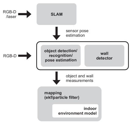
Figure 1: Block diagram of the overall system

III-A Wall and Sensor Model

We model a wall by a 2D line i.e., line on the ground-plane. Further, we assume walls are perpendicular to ground-plane. Wall is parameterized by its closest point to origin, $\mathbf{w}=(u,v)$. (Fig. 2).

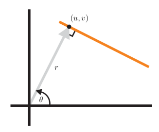
Figure 2: Model for the wall

We use the same line parameterization both in observation space and in state space. Therefore, sensor model works like point translation/rotation in 2D space $(c=\cos,s=\sin)$:

$$\mathbf{h}=\begin{bmatrix}u^{\prime}\\ v^{\prime}\\ 1\end{bmatrix}=\begin{bmatrix}c(\theta)&s(\theta)&-xc(\theta)-ys(\theta)\\ -s(\theta)&c(\theta)&xs(\theta)-yc(\theta)\\ 0&0&1\end{bmatrix}\begin{bmatrix}u\\ v\\ 1\end{bmatrix}$$ (1)

where $(x,y,\theta)$ is robot’s pose from where the wall is observed.

The inverse sensor model is

$$\mathbf{h}^{-1}=\begin{bmatrix}u\\ v\\ 1\end{bmatrix}=\begin{bmatrix}c(\theta)&-s(\theta)&x\\ s(\theta)&c(\theta)&y\\ 0&0&1\end{bmatrix}\begin{bmatrix}u^{\prime}\\ v^{\prime}\\ 1\end{bmatrix}$$ (2)

Jacobian of sensor model w.r.t walls state space is

$$\mathbf{H}=\begin{bmatrix}c(\theta)&s(\theta)\\ -s(\theta)&c(\theta)\end{bmatrix}$$ (3)

III-B Wall Detector

To detect walls ($\mathcal{L}$) from RGB-D Sensor, we use line fitting (RANSAC) on a specific row in point cloud data ($\mathcal{P}$). We choose it to be a row in upper part of the point cloud to avoid occlusion by objects. wall_detector() is shown in Algorithm 1.

Input: $\mathcal{P}$

Result: $\mathcal{L}$

1

2begin

       $\mathcal{C}=\varnothing$ ;

        /* line cluster */

       $\mathcal{P}^{\prime}\leftarrow\mathcal{P}$ ;

        /* only take a row of pointclouds */

3       $\mathcal{C}\leftarrow$ clusterByNaN ($\mathcal{P}^{\prime}$);

4       $\mathcal{L}\leftarrow$ seqLineFittingByRansac ($\mathcal{C}$);

5       return $\mathcal{L}$

6 end

7

Algorithm 1 wall_detector()

Input: $\mathcal{P}^{\prime}$

Result: $\mathcal{C}$

1 begin

2       $\mathcal{C}_{i}=\varnothing$;

3       foreach $p$ in $\mathcal{P}^{\prime}$ do

4             if isFinite ($p$) then

5                   $\mathcal{C}_{i}\leftarrow\mathcal{C}_{i}+\{p\}$;

6                   continue;

7             end if

8            

9            $\mathcal{C}\leftarrow\mathcal{C}+\{\mathcal{C}_{i}\}$;

10             $\mathcal{C}_{i}=\varnothing$;

11            

12       end foreach

13      return $\mathcal{C}$;

14      

15 end

16

Algorithm 2 clusterByNan()

Input: $\mathcal{C}$

Result: $\mathcal{L}$

1

2begin

3       foreach $\mathcal{C}_{i}$ in $\mathcal{C}$ do

4             while $\mathcal{C}_{i}\neq\varnothing$ do

5                   $\mathcal{L}_{i}$ $\leftarrow$ lineFitting ($\mathcal{C}_{i}$);

6                   removeInliers ($\mathcal{C}_{i}$);

7                   $\mathcal{L}\leftarrow\mathcal{L}+\{\mathcal{L}_{i}\}$;

8                  

9             end while

10            

11       end foreach

12      return $\mathcal{L}$

13 end

14

Algorithm 3 seqLineFittingByRansac()

RANSAC returns wall in parameter $m$ and $c$. It is straightforward to change it to point closest to origin.

$$u =\frac{-mc}{m^{2}+1}$$ (4)

$$v =\frac{c}{m^{2}+1}$$

III-C Mapping Wall with EKF

Our goal is to calculating probability density function of walls given observations ($\mathbf{z}_{1:t}$) and robot’s poses ($\mathbf{x}_{1:t}$):

$$p(\mathbf{w}_{1:M}|\mathbf{x}_{1:t},\mathbf{z}_{1:t})$$ (5)

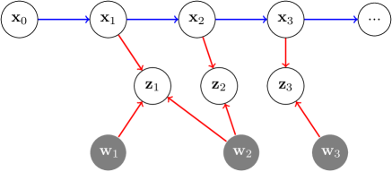
Figure 3: Dynamic Bayesian Network for walls mapping problem. Shaded nodes indicate unknown variables.

From Dynamic Bayesian Network (Fig. 3) and using concept of conditional independence, Equation 5 could be factored as

$$p(\mathbf{w}_{1:M}|\mathbf{x}_{1:t},\mathbf{z}_{1:t})=\prod_{i=1}^{M}p(\mathbf{w}_{i}|\mathbf{x}_{1:t},\mathbf{z}_{1:t})$$ (6)

It means we could calculate the posterior of landmarks from product of posteriors for individual landmark.

Within Recursive Bayesian Framework, with the Gaussian assumption of posterior ($\mathbf{w}\sim\mathcal{N}(\mathbf{\bar{w}},\Sigma_{\mathbf{w}})$), each individual landmark could be estimated using Extended Kalman Filter.

$$\mathbf{w}_{i} \leftarrow\mathbf{w}_{i}+\mathbf{K}(\mathbf{z}_{k}-\mathbf{h})$$ (7)

$$\Sigma_{\mathbf{w}} \leftarrow(\mathbf{I}-\mathbf{K}\mathbf{H})\Sigma_{\mathbf{w}}$$

with $\mathbf{K}$ is Kalman Gain

$$\mathbf{K}=\Sigma_{\mathbf{w}}\mathbf{H}^{T}(\mathbf{R}+\mathbf{H}\Sigma_{\mathbf{w}}\mathbf{H}^{T})^{-1}$$ (8)

$\mathbf{R}$ is covariance of measurement noise.

III-D Data Association

We use maximum likelihood to find whether a given observation is coming from the already observed wall. The likelihood function is defined

$$L =p(\mathbf{z}_{i,k}|\mathbf{w}_{i},\mathbf{x}_{k})$$ (9)

$$\propto\exp(-0.5\times(\mathbf{z}-\mathbf{h})^{T}\Sigma_{\mathbf{w}}^{-1}(\mathbf{z}-\mathbf{h}))$$

Because there are a small number of walls in environment, we use exhaustive search to do data association. A sensor observes a new wall whenever the maximum likelihood falls below a certain threshold.

IV Experiments

We use ROS package of grid mapping as an underlying SLAM system. We tested our system in MIT Stata Center Dataset [16].

MIT Stata Center Dataset is a very challenging dataset because it consists of indoor environment with irregular shape of rooms. There are numerous rooms without clear boundaries and walls with large windows (Fig. 4). This frequently makes wall detector fail to detect walls. Furthermore, the room sometimes have a large dimension which makes RGB-D sensor fail to reach the furthest side of its wall. This gives rather scarce wall detection rate as seen in Fig. 11 and Fig. 12.

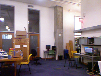
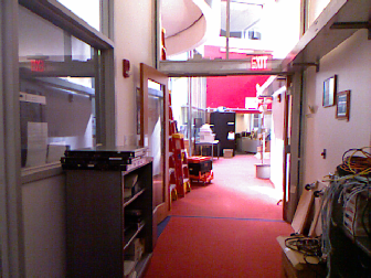
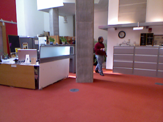
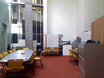
Figure 4: Example frames from MIT Stata Center Dataset

Our wall detection method is simple but it has acceptable detection performance. Fig. 7 shows detection performance of our method. Fig. 5 and Fig. 6 shows result of wall detector algorithm to two frames in dataset.

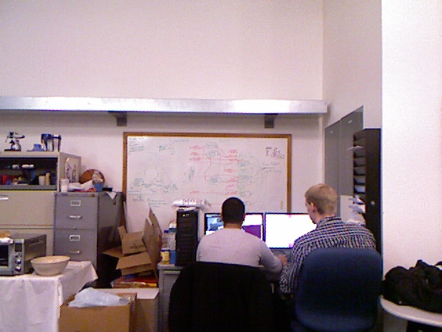
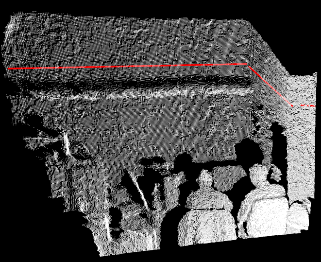
Figure 5: Wall detector algorithm successfully detects a wall in relatively simple scene

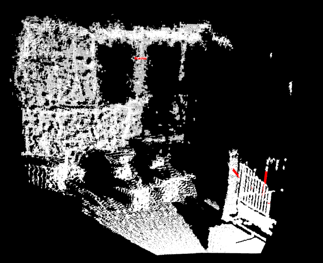
Figure 6: Challenging frame: the wall is relatively far from sensor making greater noise in pointclouds. Wall detector failed to detect large portion of the wall in the left side of the frame.

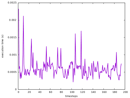
Figure 7: Execution time of wall_detector() algorithm.

Other critical component in our system is data association. Although we used exhaustive search, the number of walls never grows very large. Fig. 8 shows performance of the method.

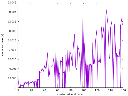
Figure 8: Data association vs number of landmarks

In EKF-based SLAM, updating the covariance matrix would be the most time consuming process. Here, our EKF is in small and constant dimension. It does not depend on the number of landmarks (Fig. 9).

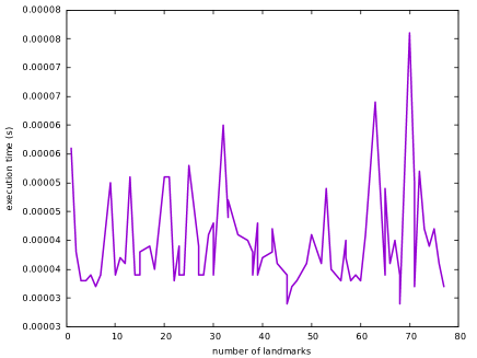
Figure 9: Execution time of EKF update vs number of landmarks

Overall, Fig. 10 show the execution time of our method plotted in timesteps. This excludes time consumed by gmapping as underlying component of our method. For the mapping result, it is shown in Fig. 11.

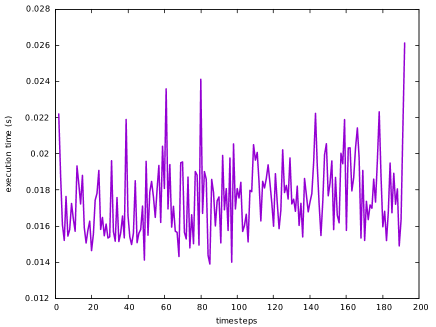
Figure 10: Execution time of our method (without gmapping time)

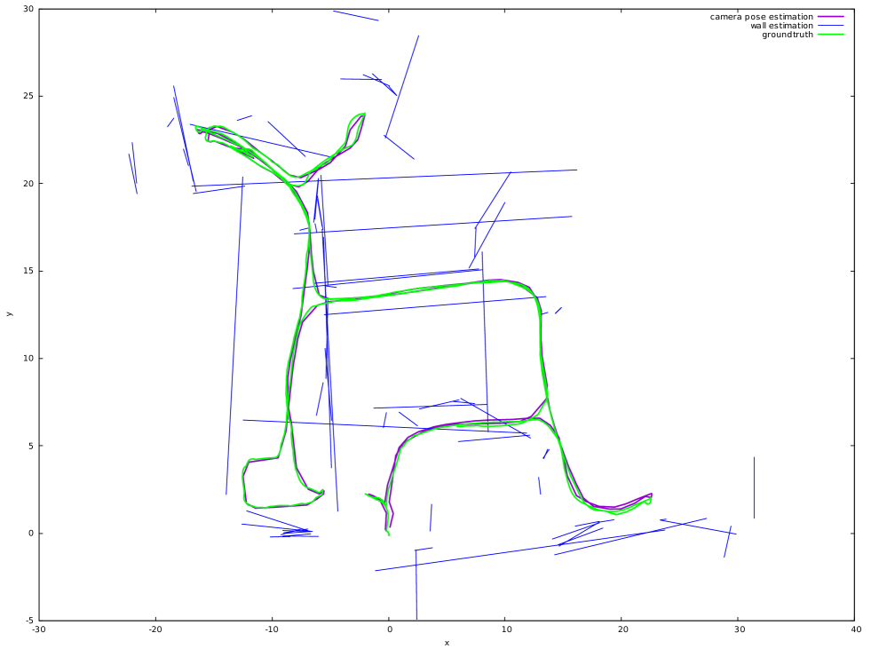
Figure 11: Result with robot’s trajectory estimation using gmapping.

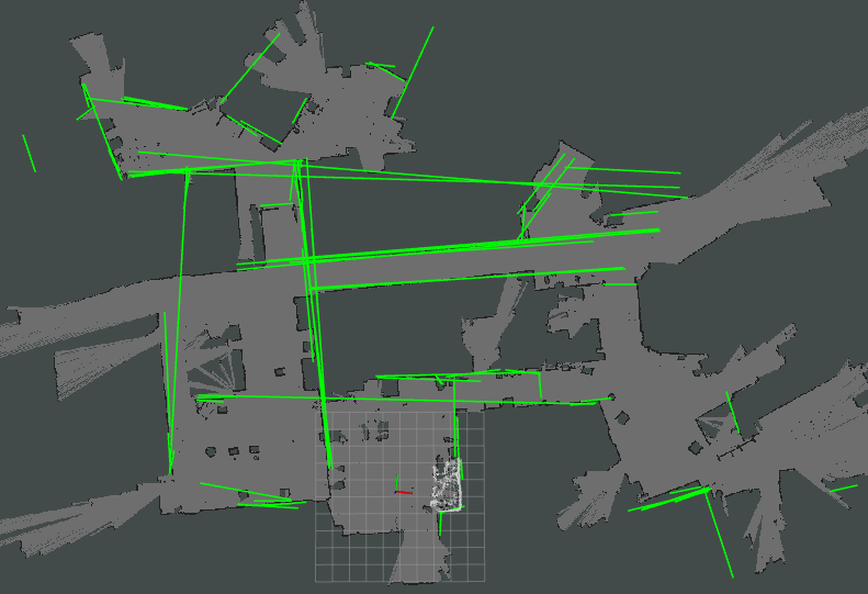
Figure 12: Result overlaid on occupancy grid from gmapping

In our experiments, we use software and hardware as listed in Table I.

TABLE I: Softwares and hardwares used in experiments

Soft/Hardwares	Specifications
Dataset	MIT Stata Center Dataset
Processor	Intel i5-3330 3GHz processor
RAM	16GB
Pointclouds library	pcl
Software framework	ROS

V Conclusion and Future Work

We seek to building a method to mapping walls in indoor environment which

1. has a simple model to represents walls configuration

2. has the capability of working online

3. has no assumption about the shape of the room

In this paper, we showed our preliminary work on wall detector from moving RGB-D sensor and showed the performance in terms of speed of execution.

Our future works would be to improve the accuracy of wall detection and implementing model of walls configurations. Further, we seek to develop a method to also map objects in environment.

References

- [1] R. O. Castle, D. J. Gawley, G. Klein, and D. W. Murray, “Towards simultaneous recognition, localization and mapping for hand-held and wearable cameras,” in Proceedings 2007 IEEE International Conference on Robotics and Automation, April 2007, pp. 4102–4107.
- [2] J. Civera, D. Gálvez-López, L. Riazuelo, J. D. Tardós, and J. Montiel, “Towards Semantic SLAM Using a Monocular Camera,” in Intelligent Robots and Systems (IROS), 2011 IEEE/RSJ International Conference on. IEEE, 2011, pp. 1277–1284.
- [3] J. Rogers, A. Trevor, C. Nieto-Granda, and H. Christensen, “Simultaneous localization and mapping with learned object recognition and semantic data association,” in 2011 IEEE/RSJ International Conference on Intelligent Robots and Systems (IROS), #sep# 2011, pp. 1264–1270.
- [4] N. Fioraio, G. Cerri, and L. D. Stefano, “Towards Semantic KinectFusion,” in Image Analysis and Processing – ICIAP 2013, ser. Lecture Notes in Computer Science, A. Petrosino, Ed. Springer Berlin Heidelberg, #sep# 2013, no. 8157, pp. 299–308.
- [5] R. Salas-Moreno, R. Newcombe, H. Strasdat, P. Kelly, and A. Davison, “SLAM++: Simultaneous Localisation and Mapping at the Level of Objects,” in 2013 IEEE Conference on Computer Vision and Pattern Recognition (CVPR), #jun# 2013, pp. 1352–1359.
- [6] D. Gálvez-López, M. Salas, J. D. Tardós, and J. M. M. Montiel, “Real-time Monocular Object SLAM,” Rob. Auton. Syst., vol. 75, pp. 435–449, 2016.
- [7] C. Cadena, L. Carlone, H. Carrillo, Y. Latif, D. Scaramuzza, J. Neira, I. Reid, and J. J. Leonard, “Past, present, and future of simultaneous localization and mapping: Toward the robust-perception age,” IEEE Transactions on Robotics, vol. 32, no. 6, pp. 1309–1332, 2016.
- [8] S. Dasgupta, K. Fang, K. Chen, and S. Savarese, “Delay: Robust spatial layout estimation for cluttered indoor scenes,” in Proceedings of the IEEE Conference on Computer Vision and Pattern Recognition, 2016, pp. 616–624.
- [9] A. Geiger and C. Wang, “Joint 3d object and layout inference from a single rgb-d image,” in German Conference on Pattern Recognition. Springer, 2015, pp. 183–195.
- [10] Z. Ren and E. B. Sudderth, “Three-dimensional object detection and layout prediction using clouds of oriented gradients,” in Proceedings of the IEEE Conference on Computer Vision and Pattern Recognition, 2016, pp. 1525–1533.
- [11] S. Y. Bao, A. Furlan, L. Fei-Fei, and S. Savarese, “Understanding the 3d layout of a cluttered room from multiple images,” in Applications of Computer Vision (WACV), 2014 IEEE Winter Conference on. IEEE, 2014, pp. 690–697.
- [12] G. Tsai and B. Kuipers, “Dynamic visual understanding of the local environment for an indoor navigating robot,” in 2012 IEEE/RSJ International Conference on Intelligent Robots and Systems (IROS), #oct# 2012, pp. 4695–4701.
- [13] A. Furlan, S. Miller, D. G. Sorrenti, L. Fei-Fei, and S. Savarese, “Free your camera: 3d indoor scene understanding from arbitrary camera motion,” in British Machine Vision Conference (BMVC), 2013, p. 9.
- [14] M. Salas, W. Hussain, A. Concha, L. Montano, J. Civera, and J. Montiel, “Layout aware visual tracking and mapping,” in Intelligent Robots and Systems (IROS), 2015 IEEE/RSJ International Conference on. IEEE, 2015, pp. 149–156.
- [15] G. Grisetti, C. Stachniss, and W. Burgard, “Improved techniques for grid mapping with rao-blackwellized particle filters,” IEEE transactions on Robotics, vol. 23, no. 1, pp. 34–46, 2007.
- [16] M. Fallon, H. Johannsson, M. Kaess, and J. J. Leonard, “The mit stata center dataset,” The International Journal of Robotics Research, vol. 32, no. 14, pp. 1695–1699, 2013.