Abstract

For the search for scalar leptons in the Minimal Supersymmetric Standard Model (MSSM) as well as for future precision analyses of these particles an accurate knowledge of their production and decay properties is mandatory. We evaluate the cross sections for the slepton production at $e^{+}e^{-}$ colliders in the MSSM with complex parameters (cMSSM). The evaluation is based on a full one-loop calculation of the production mechanisms $e^{+}e^{-}\to\tilde{l}_{gs}\tilde{l}_{gs^{\prime}}$ including soft and hard photon radiation. The dependence of the slepton production cross sections on the relevant cMSSM parameters is analyzed numerically. We find sizable contributions to many production cross sections. They amount to roughly $15\,\%$ of the tree-level results but can go up to $40\,\%$ or higher in extreme cases. Also the complex phase dependence of the one-loop corrections for charged slepton production was found non-negligible. The full one-loop contributions are thus crucial for physics analyses at a future linear $e^{+}e^{-}$ collider such as the ILC or CLIC.

1 Introduction

One of the important tasks at the LHC is to search for physics beyond the Standard Model (SM), where the Minimal Supersymmetric Standard Model (MSSM) [2, 3, 4, 5] is one of the leading candidates. Two related important tasks are the investigation of the mechanism of electroweak symmetry breaking, including the identification of the underlying physics of the Higgs boson discovered at $\sim 125\,\,\mathrm{GeV}$ [6, 7], as well as the production and measurement of the properties of Cold Dark Matter (CDM). Here the MSSM offers a natural candidate for CDM, the Lightest Supersymmetric Particle (LSP), the lightest neutralino, $\tilde{\chi}_{1}^{0}$ [8, 9] (see below). These three (related) tasks will be the top priority in the future program of particle physics.

Supersymmetry (SUSY) predicts two scalar partners for all SM fermions as well as fermionic partners to all SM bosons. Contrary to the case of the SM, in the MSSM two Higgs doublets are required. This results in five physical Higgs bosons instead of the single Higgs boson in the SM. These are the light and heavy ${{\cal CP}}$-even Higgs bosons, $h$ and $H$, the ${{\cal CP}}$-odd Higgs boson, $A$, and the charged Higgs bosons, $H^{\pm}$. In the MSSM with complex parameters (cMSSM) the three neutral Higgs bosons mix [10, 11, 12, 13, 14], giving rise to the ${{\cal CP}}$-mixed states $h_{1},h_{2},h_{3}$. The neutral SUSY partners of the (neutral) Higgs and electroweak gauge bosons are the four neutralinos, $\tilde{\chi}_{1,2,3,4}^{0}$. The corresponding charged SUSY partners are the charginos, $\tilde{\chi}_{1,2}^{\pm}$.

If SUSY is realized in nature and the scalar quarks and/or the gluino are in the kinematic reach of the (HL-)LHC, it is expected that these strongly interacting particles are eventually produced and studied. On the other hand, SUSY particles that interact only via the electroweak force, e.g., the scalar leptons, have a much smaller production cross section at the LHC. Correspondingly, the LHC discovery potential as well as the current experimental bounds are substantially weaker [15, 16].

At a (future) $e^{+}e^{-}$ collider sleptons, depending on their masses and the available center-of-mass energy, could be produced and analyzed in detail. Corresponding studies can be found for the ILC in Refs. [17, 18, 19, 20, 21, 22] and for CLIC in Refs. [23, 24, 22]. (Results on the combination of LHC and ILC results can be found in Refs. [25, 26, 27].) Such precision studies will be crucial to determine their nature and the underlying (SUSY) parameters.

In order to yield a sufficient accuracy, one-loop corrections to the various slepton production and decay modes have to be considered. Full one-loop calculations in the cMSSM to (heavy) scalar tau decays was evaluated in Ref. [28], where the calculation can easily be taken over to other slepton decays. Sleptons can also be produced in SUSY cascade decays. Full one-loop evaluations in the cMSSM exist for the corresponding decays of Higgs bosons [29] as well as from charginos and neutralinos [30, 31, 32, 33]. In this paper we take the next step and concentrate on the slepton production at $e^{+}e^{-}$ colliders, i.e. we calculate

$$\sigma(e^{+}e^{-}\to\mathrm{\tilde{e}}^{\pm}_{gs}\mathrm{\tilde{e}}^{\mp}_{gs^{\prime}}) s,s^{\prime}=1,2\,,$$ (1)

$$\sigma(e^{+}e^{-}\to\tilde{\nu}_{g}\tilde{\nu}_{g}^{*}) g=1,2,3\,,$$ (2)

with $\mathrm{\tilde{e}}_{gs}=\{\tilde{e}_{s},\tilde{\mu}_{s},\tilde{\tau}_{s}\}$, $\tilde{\nu}_{g}=\{\tilde{\nu}_{e},\tilde{\nu}_{\mu},\tilde{\nu}_{\tau}\}$, generation index $g$ and slepton index $s$. Our evaluation of the two channels (1) and (2) is based on a full one-loop calculation, i.e. including electroweak (EW) corrections, as well as soft, hard and collinear QED radiation. The renormalization scheme employed is the same one as for the decay of sleptons [28]. Consequently, the predictions for the production and decay can be used together in a consistent manner.

Results for the cross sections (1) and (2) at various levels of sophistication have been obtained over the last three decades. Tree-level results were published for $e^{+}e^{-}\to\mathrm{\tilde{e}}^{\pm}_{gs}\mathrm{\tilde{e}}^{\mp}_{gs^{\prime}}$ and $e^{+}e^{-}\to\tilde{\nu}_{g}\tilde{\nu}_{g}^{*}$ in the MSSM with real parameters (rMSSM) in Ref. [34], and later in a specific supergravity (SUGRA) model in Ref. [35]. Tree-level results in the cMSSM were published only for the process $\mu^{+}\mu^{-}\to{\tilde{\tau}_{s}}^{\pm}{\tilde{\tau}_{s^{\prime}}}^{\mp}$ in Ref. [36]. Several works dealt with the slepton production cross section at threshold [37, 38], also taking into account the electron/positron polarization [39], which is outside the scope of this article. Full one-loop corrections in the rMSSM were presented for $e^{+}e^{-}\to{\tilde{e}_{s}}^{\pm}{\tilde{e}_{s^{\prime}}}^{\mp},{\tilde{\mu}_{s}}^{\pm}{\tilde{\mu}_{s^{\prime}}}^{\mp}$ [40] and for $e^{+}e^{-}\to\tilde{\nu}_{g}\tilde{\nu}_{g}^{*}$ [41]. Using a renormalization scheme close to ours (see below), stop, sbottom, and stau production at $e^{+}e^{-}$ colliders was evaluated in Ref. [42] in the rMSSM at the full one-loop level. Third generation sfermion production at the full one-loop level in the rMSSM, including staus and tau sneutrinos were presented in Refs. [43, 44, 45].

In this paper we present for the first time a full and consistent one-loop calculation in the cMSSM for scalar lepton production at $e^{+}e^{-}$ colliders. We take into account soft, hard and collinear QED radiation and the treatment of collinear divergences. Again, here it is crucial to stress that the same renormalization scheme as for the decay of sleptons [28] (and for slepton production from Higgs boson decays [29] as well as from chargino and neutralino decays [30, 31, 32, 33]) has been used. Consequently, the predictions for the production and decay can be used together in a consistent manner (e.g., in a global phenomenological analysis of the slepton sector at the one-loop level). We analyze all processes w.r.t. the most relevant parameters, including the relevant complex phases. In this way we go substantially beyond the existing analyses (see above). In Sect. 2 we briefly review the renormalization of the relevant sectors of the cMSSM and give details as regards the calculation. In Sect. 3 various comparisons with results from other groups are given. The numerical results for the production channels (1) and (2) are presented in Sect. 4. The conclusions can be found in Sect. 5.

Prolegomena

We use the following short-hands in this paper:

• FeynTools $\equiv$ FeynArts + FormCalc + LoopTools.

• full = tree + loop.

• $s_{\mathrm{w}}\equiv\sin\theta_{W}$, $c_{\mathrm{w}}\equiv\cos\theta_{W}$.

• $t_{\beta}\equiv\tan\beta$.

They will be further explained in the text below.

2 Calculation of diagrams

In this section we give some details regarding the renormalization procedure and the calculation of the tree-level and higher-order corrections to the production of sleptons in $e^{+}e^{-}$ collisions. The diagrams and corresponding amplitudes have been obtained with FeynArts (version 3.9) [46, 47, 48], using our MSSM model file (including the MSSM counterterms) of Ref. [49]. The further evaluation has been performed with FormCalc (version 9.5) and LoopTools (version 2.14) [50, 51].

2.1 The complex MSSM

The cross sections (1) and (2) are calculated at the one-loop level, including soft, hard and collinear QED radiation; see the next section. This requires the simultaneous renormalization of the gauge-boson sector, the lepton sector as well as the slepton sector of the cMSSM. We give a few relevant details as regards these sectors and their renormalization. More details and the application to Higgs-boson and SUSY particle decays can be found in Refs. [29, 52, 49, 53, 54, 55, 56, 28, 30, 31, 32, 33]. Similarly, the application to Higgs-boson and chargino/neutralino production cross sections at $e^{+}e^{-}$ colliders are given in Refs. [57, 58, 59].

The renormalization of the fermion and gauge-boson sector follows strictly Ref. [49] and the references therein (see especially Ref. [60]). This defines in particular the counterterm $\delta t_{\beta}$, as well as the counterterms for the $Z$ boson mass, $\delta M_{Z}^{2}$, and for the sine of the weak mixing angle, $\delta s_{\mathrm{w}}$ (with $s_{\mathrm{w}}=\sqrt{1-c_{\mathrm{w}}^{2}}=\sqrt{1-M_{W}^{2}/M_{Z}^{2}}$, where $M_{W}$ and $M_{Z}$ denote the $W$ and $Z$ boson masses, respectively). For the fermion sector we use the default values as given in Ref. [49].

The renormalization of the slepton sector is implemented just as the “$m_{b},A_{b}$ $\smash{\overline{\mathrm{DR}}}$” (RS2) scheme of Refs. [53, 54, 55], but extended to sleptons and all generations, also including the corresponding sfermion shifts.

The up-type squarks ($\mathrm{\tilde{u}}_{g}=\{\tilde{u},\tilde{c},\tilde{t}\}$), the neutrino-type sleptons ($\tilde{\nu}_{g}=\{\tilde{\nu}_{e},\tilde{\nu}_{\mu},\tilde{\nu}_{\tau}\}$), the down-type squarks ($\mathrm{\tilde{d}}_{g}=\{\tilde{d},\tilde{s},\tilde{b}\}$), and the electron-type sleptons ($\mathrm{\tilde{e}}_{g}=\{\tilde{e},\tilde{\mu},\tilde{\tau}\}$) are renormalized on-shell. The latter two via option $\mathcal{O}2$ of Refs. [53, 54].

The “$m_{b},A_{b}$ $\smash{\overline{\mathrm{DR}}}$” scheme of Refs. [53, 54, 55], extended to all generations is herein after referred to as mixed scheme, of course not to be confused with the mixed scheme of Ref. [49].

The schemes affecting $\mathrm{\tilde{e}}_{g}$ and $\mathrm{\tilde{d}}_{g}$ are chosen with the variable $SfScheme[t, $\mathit{g}$]:

$SfScheme[2, $$\mathit{g} A_{\mathrm{e}_{g}} \smash{\overline{\mathrm{DR}}}$$] = DR[s] mixed scheme with

$SfScheme[4, $$\mathit{g} A_{\mathrm{d}_{g}} \smash{\overline{\mathrm{DR}}}$$] = DR[s] mixed scheme with

The sfermions are on-shell, i.e. the sfermion index $\mathit{s}$ runs over both values 1, 2.

dMSfsq1[1, 1, 1, $$\mathit{g} \equiv{} \delta m_{\tilde{\nu}_{g1}}^{2} =\mathop{\widetilde{\mathrm{Re}}}\bigl{(}\Sigma_{\tilde{\nu}_{g}}(m_{\tilde{\nu}_{g1}}^{2})\bigr{)}_{11}\,,$$] (4a)

dMSfsq1[$$\mathit{s} \mathit{s} \mathit{g} \equiv{} \delta m_{\mathrm{\tilde{e}}_{gs}}^{2} =\mathop{\widetilde{\mathrm{Re}}}\bigl{(}\Sigma_{\mathrm{\tilde{e}}_{g}}(m_{\mathrm{\tilde{e}}_{gs}}^{2})\bigr{)}_{ss}\,,$$, , 2, ] (4b)

dMSfsq1[$$\mathit{s} \mathit{s} \mathit{g} \equiv{} \delta m_{\mathrm{\tilde{u}}_{gs}}^{2} =\mathop{\widetilde{\mathrm{Re}}}\bigl{(}\Sigma_{\mathrm{\tilde{u}}_{g}}(m_{\mathrm{\tilde{u}}_{gs}}^{2})\bigr{)}_{ss}\,,$$, , 3, ] (4c)

dMSfsq1[$$\mathit{s} \mathit{s} \mathit{g} \equiv{} \delta m_{\mathrm{\tilde{d}}_{gs}}^{2} =\mathop{\widetilde{\mathrm{Re}}}\bigl{(}\Sigma_{\mathrm{\tilde{d}}_{g}}(m_{\mathrm{\tilde{d}}_{gs}}^{2})\bigr{)}_{ss}\,.$$, , 4, ] (4d)

The non-diagonal entries of the up-type mass matrix are determined by [53, 54]

dMSfsq1[1, 2, 3, $$\mathit{g} \equiv\delta Y_{\mathrm{u}_{g}}=\frac{1}{2}\mathop{\widetilde{\mathrm{Re}}}\bigl{(}\Sigma_{\mathrm{\tilde{u}}_{g}}(m_{\mathrm{\tilde{u}}_{g1}}^{2})+\Sigma_{\mathrm{\tilde{u}}_{g}}(m_{\mathrm{\tilde{u}}_{g2}}^{2})\bigr{)}_{12}\,,$$] (4e)

dMSfsq1[2, 1, 3, $$\mathit{g} \equiv\delta Y_{\mathrm{u}_{g}}^{*}=\frac{1}{2}\mathop{\widetilde{\mathrm{Re}}}\bigl{(}\Sigma_{\mathrm{\tilde{u}}_{g}}(m_{\mathrm{\tilde{u}}_{g1}}^{2})+\Sigma_{\mathrm{\tilde{u}}_{g}}(m_{\mathrm{\tilde{u}}_{g2}}^{2})\bigr{)}_{21}\,.$$] (4f)

For clarity of notation we furthermore define the auxiliary constants

$$\texttt{dMsq12Sf1[2,\,$\mathit{g}$]}\equiv\delta M_{\mathrm{\tilde{e}}_{g},12}^{2} =m_{\mathrm{e}_{g}}(\delta A_{\mathrm{e}_{g}}^{*}-\mu\,\delta t_{\beta}-t_{\beta}\,\delta\mu)+(A_{\mathrm{e}_{g}}^{*}-\mu\,t_{\beta})\,\delta m_{\mathrm{e}_{g}}\,,$$ (5a)

$$\texttt{dMsq12Sf1[4,\,$\mathit{g}$]}\equiv\delta M_{\mathrm{\tilde{d}}_{g},12}^{2} =m_{\mathrm{d}_{g}}(\delta A_{\mathrm{d}_{g}}^{*}-\mu\,\delta t_{\beta}-t_{\beta}\,\delta\mu)+(A_{\mathrm{d}_{g}}^{*}-\mu\,t_{\beta})\,\delta m_{\mathrm{d}_{g}}\,.$$ (5b)

For the bottom quark we choose: $\delta m_{b}=\delta m_{b}^{\smash{\overline{\mathrm{DR}}}}$.

In the mixed scheme the down-type off-diagonal mass counterterms are related as

dMSfsq1[1, 2, 2, $$\mathit{g} \equiv\delta Y_{\mathrm{e}_{g}}=\frac{1}{|U^{\mathrm{\tilde{e}}_{g}}_{11}|^{2}-|U^{\mathrm{\tilde{e}}_{g}}_{12}|^{2}}\Bigl{\{}U^{\mathrm{\tilde{e}}_{g}}_{11}U^{\mathrm{\tilde{e}}_{g}*}_{21}\bigl{(}\delta m_{\mathrm{\tilde{e}}_{g1}}^{2}-\delta m_{\mathrm{\tilde{e}}_{g2}}^{2}\bigr{)}+{}$$] (6a)

$$\kern 120.00018ptU^{\mathrm{\tilde{e}}_{g}}_{11}U^{\mathrm{\tilde{e}}_{g}*}_{22}\delta M_{\mathrm{\tilde{e}}_{g},12}^{2}-U^{\mathrm{\tilde{e}}_{g}}_{12}U^{\mathrm{\tilde{e}}_{g}*}_{21}\delta M_{\mathrm{\tilde{e}}_{g},12}^{2*}\Bigr{\}}\,,$$

dMSfsq1[2, 1, 2, $$\mathit{g} =\delta Y_{\mathrm{e}_{g}}^{*}\,,$$] (6b)

dMSfsq1[1, 2, 4, $$\mathit{g} \equiv\delta Y_{\mathrm{d}_{g}}=\frac{1}{|U^{\mathrm{\tilde{d}}_{g}}_{11}|^{2}-|U^{\mathrm{\tilde{d}}_{g}}_{12}|^{2}}\Bigl{\{}U^{\mathrm{\tilde{d}}_{g}}_{11}U^{\mathrm{\tilde{d}}_{g}*}_{21}\bigl{(}\delta m_{\mathrm{\tilde{d}}_{g1}}^{2}-\delta m_{\mathrm{\tilde{d}}_{g2}}^{2}\bigr{)}+{}$$] (6c)

$$\kern 120.00018ptU^{\mathrm{\tilde{d}}_{g}}_{11}U^{\mathrm{\tilde{d}}_{g}*}_{22}\delta M_{\mathrm{\tilde{d}}_{g},12}^{2}-U^{\mathrm{\tilde{d}}_{g}}_{12}U^{\mathrm{\tilde{d}}_{g}*}_{21}\delta M_{\mathrm{\tilde{d}}_{g},12}^{2*}\Bigr{\}}\,,$$

dMSfsq1[2, 1, 4, $$\mathit{g} =\delta Y_{\mathrm{d}_{g}}^{*}\,.$$] (6d)

The trilinear couplings $A_{f_{tg}}\equiv\bigl{(}\mathbf{A}_{f_{t}}\bigr{)}_{gg}$ are renormalized by

dAf1[2, $$\mathit{g} \mathit{g} \equiv\delta A_{\mathrm{e}_{g}} =\biggl{\{}\frac{1}{m_{\mathrm{e}_{g}}}\Bigl{[}\begin{aligned} &U^{\mathrm{\tilde{e}}_{g}}_{11}U^{\mathrm{\tilde{e}}_{g}*}_{12}(\delta m_{\mathrm{\tilde{e}}_{g1}}^{2}-\delta m_{\mathrm{\tilde{e}}_{g2}}^{2})+{}\\ &U^{\mathrm{\tilde{e}}_{g}}_{11}U^{\mathrm{\tilde{e}}_{g}*}_{22}\delta Y_{\mathrm{e}_{g}}^{*}+U^{\mathrm{\tilde{e}}_{g}*}_{12}U^{\mathrm{\tilde{e}}_{g}}_{21}\delta Y_{\mathrm{e}_{g}}-(A_{\mathrm{e}_{g}}-\mu^{*}t_{\beta})\,\delta m_{\mathrm{e}_{g}}\hbox to0.0pt{$\Bigr{]}+{}$\hss}\end{aligned}$$, ] (7a)

$$\qquad t_{\beta}\,\delta\mu^{*}+\mu^{*}\delta t_{\beta}\biggr{\}}_{\mathrm{[div]}}\,,$$

dAf1[3, $$\mathit{g} \mathit{g} \equiv\delta A_{\mathrm{u}_{g}} =\frac{1}{m_{\mathrm{u}_{g}}}\Bigl{[}\hbox to0.0pt{$\begin{aligned} &U^{\mathrm{\tilde{u}}_{g}}_{11}U^{\mathrm{\tilde{u}}_{g}*}_{12}(\delta m_{\mathrm{\tilde{u}}_{g1}}^{2}-\delta m_{\mathrm{\tilde{u}}_{g2}}^{2})+{}\\ &U^{\mathrm{\tilde{u}}_{g}}_{11}U^{\mathrm{\tilde{u}}_{g}*}_{22}\delta Y_{\mathrm{u}_{g}}^{*}+U^{\mathrm{\tilde{u}}_{g}*}_{12}U^{\mathrm{\tilde{u}}_{g}}_{21}\delta Y_{\mathrm{u}_{g}}-\bigl{(}A_{\mathrm{u}_{g}}-\mu^{*}/t_{\beta}\bigr{)}\,\delta m_{\mathrm{u}_{g}}\hbox to0.0pt{$\Bigr{]}+{}$\hss}\end{aligned}$\hss}$$, ] (7b)

$$\qquad\delta\mu^{*}/t_{\beta}-\mu^{*}\delta t_{\beta}/t_{\beta}^{2}\,,$$

dAf1[4, $$\mathit{g} \mathit{g} \equiv\delta A_{\mathrm{d}_{g}} =\biggl{\{}\frac{1}{m_{\mathrm{d}_{g}}}\Bigl{[}\hbox to0.0pt{$\begin{aligned} &U^{\mathrm{\tilde{d}}_{g}}_{11}U^{\mathrm{\tilde{d}}_{g}*}_{12}(\delta m_{\mathrm{\tilde{d}}_{g1}}^{2}-\delta m_{\mathrm{\tilde{d}}_{g2}}^{2})+{}\\ &U^{\mathrm{\tilde{d}}_{g}}_{11}U^{\mathrm{\tilde{d}}_{g}*}_{22}\delta Y_{\mathrm{d}_{g}}^{*}+U^{\mathrm{\tilde{d}}_{g}*}_{12}U^{\mathrm{\tilde{d}}_{g}}_{21}\delta Y_{\mathrm{d}_{g}}-(A_{\mathrm{d}_{g}}-\mu^{*}t_{\beta})\,\delta m_{\mathrm{d}_{g}}\hbox to0.0pt{$\Bigr{]}+{}$\hss}\end{aligned}$\hss}$$, ] (7c)

$$\qquad t_{\beta}\,\delta\mu^{*}+\mu^{*}\delta t_{\beta}\biggr{\}}_{\mathrm{[div]}}\,,$$

where the subscripted [div] means to take the divergent part in the mixed scheme only, to effect $\smash{\overline{\mathrm{DR}}}$ renormalization of $A_{\mathrm{e}_{g}}$ and $A_{\mathrm{d}_{g}}$ [53, 54].

The squark and slepton $Z$-factors are derived in the OS scheme and can be found in Section 3.6.1 and 3.6.2 of Ref. [49].

As now all the sfermion masses are renormalized as on-shell an explicit restoration of the $SU(2)_{L}$ relation is needed. Requiring the $SU(2)_{L}$ relation to be valid at the one-loop level induces the following shifts in the soft SUSY-breaking parameters:

$$M_{\tilde{L}}^{2}(\mathrm{\tilde{e}}_{g}) =M_{\tilde{L}}^{2}(\tilde{\nu}_{g})+\delta M_{\tilde{L}}^{2}(\tilde{\nu}_{g})-\delta M_{\tilde{L}}^{2}(\mathrm{\tilde{e}}_{g})\,,$$ (8)

$$M_{\tilde{Q}}^{2}(\mathrm{\tilde{d}}_{g}) =M_{\tilde{Q}}^{2}(\mathrm{\tilde{u}}_{g})+\delta M_{\tilde{Q}}^{2}(\mathrm{\tilde{u}}_{g})-\delta M_{\tilde{Q}}^{2}(\mathrm{\tilde{d}}_{g})$$ (9)

with

$$\delta M_{\tilde{L},\tilde{Q}}^{2}(\tilde{f}) =|U^{\tilde{f}}_{11}|^{2}\delta m_{\tilde{f}_{1}}^{2}+|U^{\tilde{f}}_{12}|^{2}\delta m_{\tilde{f}_{2}}^{2}-U^{\tilde{f}}_{22}U^{\tilde{f}*}_{12}\delta Y_{f}-U^{\tilde{f}}_{12}U^{\tilde{f}*}_{22}\delta Y_{f}^{*}-2m_{f}\delta m_{f}$$

$$\quad+M_{Z}^{2}\,c_{2\beta}\,Q_{f}\,\delta s_{\mathrm{w}}^{2}-(I_{f}^{3}-Q_{f}s_{\mathrm{w}}^{2})(c_{2\beta}\,\delta M_{Z}^{2}+M_{Z}^{2}\,\delta c_{2\beta})\,.$$ (10)

Now $M_{\tilde{L}}^{2}(\mathrm{\tilde{e}}_{g})$ and $M_{\tilde{Q}}^{2}(\mathrm{\tilde{d}}_{g})$ are used in the scalar electron- and down-type mass matrix instead of the parameters $M_{\tilde{L},\tilde{Q}}^{2}$ in the sfermion mass matrix when calculating the values of $m_{\mathrm{\tilde{e}}_{gs}}$ and $m_{\mathrm{\tilde{d}}_{gs}}$. However, with this procedure, both ($s=1,2$) sfermion masses are shifted, which contradicts our choice of independent parameters. To keep this choice, also the right-handed soft SUSY-breaking mass parameters $M_{\tilde{E},\tilde{D}}$ receive a shift:

$$M_{\tilde{E}}^{2} =\frac{m_{\mathrm{e}_{g}}^{2}\,|A_{\mathrm{e}_{g}}^{*}-\mu\,t_{\beta}|^{2}}{M_{\tilde{L}}^{2}(\mathrm{\tilde{e}}_{g})+m_{\mathrm{e}_{g}}^{2}+M_{Z}^{2}c_{2\beta}(I_{\mathrm{e}_{g}}^{3}-Q_{\mathrm{e}_{g}}s_{\mathrm{w}}^{2})-m_{\mathrm{\tilde{e}}_{gs}}^{2}}-m_{\mathrm{e}_{g}}^{2}-M_{Z}^{2}c_{2\beta}Q_{\mathrm{e}_{g}}s_{\mathrm{w}}^{2}+m_{\mathrm{\tilde{e}}_{gs}}^{2}\,,$$ (11)

$$M_{\tilde{D}}^{2} =\frac{m_{\mathrm{d}_{g}}^{2}\,|A_{\mathrm{d}_{g}}^{*}-\mu\,t_{\beta}|^{2}}{M_{\tilde{Q}}^{2}(\mathrm{\tilde{d}}_{g})+m_{\mathrm{d}_{g}}^{2}+M_{Z}^{2}c_{2\beta}(I_{\mathrm{d}_{g}}^{3}-Q_{\mathrm{d}_{g}}s_{\mathrm{w}}^{2})-m_{\mathrm{\tilde{d}}_{gs}}^{2}}-m_{\mathrm{d}_{g}}^{2}-M_{Z}^{2}c_{2\beta}Q_{\mathrm{d}_{g}}s_{\mathrm{w}}^{2}+m_{\mathrm{\tilde{d}}_{gs}}^{2}$$ (12)

with our choice of mass ordering, $m_{\tilde{f}_{1}}<m_{\tilde{f}_{2}}$, we have

$$s =\left\{\begin{array}[]{rl}1&\text{for }M_{\tilde{L}}^{2}>M_{\tilde{E}}^{2}\text{ and/or }M_{\tilde{Q}}^{2}>M_{\tilde{D}}^{2}\,,\\ 2&\text{for }M_{\tilde{E}}^{2}>M_{\tilde{L}}^{2}\text{ and/or }M_{\tilde{D}}^{2}>M_{\tilde{Q}}^{2}\,.\end{array}\right.$$ (15)

Taking into account the shift Eq. (11) in $M_{\tilde{E}}$ and Eq. (12) in $M_{\tilde{D}}$, up to one-loop order, the new resulting mass parameters $m_{\mathrm{\tilde{e}}_{gs}}$ and $m_{\mathrm{\tilde{d}}_{gs}}$ are the same as the on-shell masses:

$$\big{(}m_{\mathrm{\tilde{e}}_{gs}}^{\mathrm{OS}}\big{)}^{2} =\big{(}m_{\mathrm{\tilde{e}}_{gs}}\big{)}^{2}+\big{(}\delta m_{\mathrm{\tilde{e}}_{gs}}^{\text{dep.}}\big{)}^{2}-\mathop{\widetilde{\mathrm{Re}}}\bigl{(}\Sigma_{\mathrm{\tilde{e}}_{g}}(m_{\mathrm{\tilde{e}}_{gs}}^{2})\bigr{)}_{ss}\,,$$ (16)

$$\big{(}m_{\mathrm{\tilde{d}}_{gs}}^{\mathrm{OS}}\big{)}^{2} =\big{(}m_{\mathrm{\tilde{d}}_{gs}}\big{)}^{2}+\big{(}\delta m_{\mathrm{\tilde{d}}_{gs}}^{\text{dep.}}\big{)}^{2}-\mathop{\widetilde{\mathrm{Re}}}\bigl{(}\Sigma_{\mathrm{\tilde{d}}_{g}}(m_{\mathrm{\tilde{d}}_{gs}}^{2})\bigr{)}_{ss}$$ (17)

where $\delta m_{\mathrm{\tilde{e}}_{gs}}^{\text{dep.}}$ and $\delta m_{\mathrm{\tilde{d}}_{gs}}^{\text{dep.}}$ are the dependent mass counterterms.

A slightly different slepton sector renormalization is also described in detail in Ref. [49] and references therein.

2.2 Contributing diagrams

Sample diagrams for the process $e^{+}e^{-}\to\mathrm{\tilde{e}}^{\pm}_{gs}\mathrm{\tilde{e}}^{\mp}_{gs^{\prime}}$ and $e^{+}e^{-}\to\tilde{\nu}_{g}\tilde{\nu}_{g}^{*}$ are shown in Fig. 1. Not shown are the diagrams for real (hard and soft) photon radiation. They are obtained from the corresponding tree-level diagrams by attaching a photon to the (incoming/outgoing) electron or slepton. The internal particles in the generically depicted diagrams in Fig. 1 are labeled as follows: $F$ can be a SM fermion $f$, chargino $\tilde{\chi}_{c}^{\pm}$ or neutralino $\tilde{\chi}_{n}^{0}$; $S$ can be a sfermion $\tilde{f}_{s}$ or a Higgs (Goldstone) boson $h^{0},H^{0},A^{0},H^{\pm}$ ($G,G^{\pm}$); $U$ denotes the ghosts $u_{V}$; $V$ can be a photon $\gamma$ or a massive SM gauge boson, $Z$ or $W^{\pm}$. We have neglected all electron–Higgs couplings and terms proportional to the electron mass whenever this is safe, i.e. except when the electron mass appears in negative powers or in loop integrals. We have verified numerically that these contributions are indeed totally negligible. For internally appearing Higgs bosons no higher-order corrections to their masses or couplings are taken into account; these corrections would correspond to effects beyond one-loop order.

Moreover, in general, in Fig. 1 we have omitted diagrams with self-energy type corrections of external (on-shell) particles. While the contributions from the real parts of the loop functions are taken into account via the renormalization constants defined by OS renormalization conditions, the contributions coming from the imaginary part of the loop functions can result in an additional (real) correction if multiplied by complex parameters. In the analytical and numerical evaluation, these diagrams have been taken into account via the prescription described in Ref. [49].

Figure 1: Generic tree, self-energy, vertex, box, and counterterm diagrams for the process $e^{+}e^{-}\to\tilde{l}_{gs}\tilde{l}_{gs^{\prime}}$ ($\tilde{l}_{gs}=\{\mathrm{\tilde{e}}_{gs},\tilde{\nu}_{g}\};\;g=1,2,3;\;s,s^{\prime}=1,2$). The additional diagrams, which occur only in the case of first generation slepton production, are denoted with $\tilde{l}_{1s}$. $F$ can be a SM fermion, chargino or neutralino; $S$ can be a sfermion or a Higgs/Goldstone boson; $V$ can be a $\gamma$, $Z$ or $W^{\pm}$. It should be noted that electron–Higgs couplings are neglected.

Within our one-loop calculation we neglect finite width effects that can help to cure threshold singularities. Consequently, in the close vicinity of those thresholds our calculation does not give a reliable result. Switching to a complex mass scheme [61] would be another possibility to cure this problem, but its application is beyond the scope of our paper.

The tree-level formulas $\sigma_{\text{tree}}(e^{+}e^{-}\to\mathrm{\tilde{e}}^{\pm}_{gs}\mathrm{\tilde{e}}^{\mp}_{gs^{\prime}})$ and $\sigma_{\text{tree}}(e^{+}e^{-}\to\tilde{\nu}_{g}\tilde{\nu}_{g}^{*})$ are given in Refs. [35, 37] and Ref. [41], respectively. Concerning our evaluation of $\sigma(e^{+}e^{-}\to\mathrm{\tilde{e}}^{\pm}_{gs}\mathrm{\tilde{e}}^{\mp}_{gs^{\prime}})$ we define:

$$\sigma(e^{+}e^{-}\to\mathrm{\tilde{e}}^{\pm}_{gs}\mathrm{\tilde{e}}^{\mp}_{gs^{\prime}})\equiv\sigma(e^{+}e^{-}\to\mathrm{\tilde{e}}^{+}_{gs}\mathrm{\tilde{e}}^{-}_{gs^{\prime}})+\sigma(e^{+}e^{-}\to\mathrm{\tilde{e}}^{-}_{gs}\mathrm{\tilde{e}}^{+}_{gs^{\prime}})\qquad\forall\;s\neq s^{\prime}\,,$$ (18)

if not indicated otherwise. Differences between the two charge conjugated processes can appear at the loop level when complex parameters are taken into account, as will be discussed in Sect. 4.2.

2.3 Ultraviolet, infrared and collinear divergences

As regularization scheme for the UV divergences we have used constrained differential renormalization [62], which has been shown to be equivalent to dimensional reduction [63, 64] at the one-loop level [50, 51]. Thus the employed regularization scheme preserves SUSY [65, 66] and guarantees that the SUSY relations are kept intact, e.g., that the gauge couplings of the SM vertices and the Yukawa couplings of the corresponding SUSY vertices also coincide to one-loop order in the SUSY limit. Therefore no additional shifts, which might occur when using a different regularization scheme, arise. All UV divergences cancel in the final result.

Soft photon emission implies numerical problems in the phase space integration of radiative processes. The phase space integral diverges in the soft energy region where the photon momentum becomes very small, leading to infrared (IR) singularities. Therefore the IR divergences from diagrams with an internal photon have to cancel with the ones from the corresponding real soft radiation. We have included the soft photon contribution via the code already implemented in FormCalc following the description given in Ref. [67]. The IR divergences arising from the diagrams involving a photon are regularized by introducing a photon mass parameter, $\lambda$. All IR divergences, i.e. all divergences in the limit $\lambda\to 0$, cancel once virtual and real diagrams for one process are added. We have numerically checked that our results do not depend on $\lambda$ or on $\Delta E=\delta_{s}E=\delta_{s}\sqrt{s}/2$ defining the energy cut that separates the soft from the hard radiation. As one can see from the example in Fig. 2 this holds for several orders of magnitude. Our numerical results below have been obtained for fixed $\delta_{s}=10^{-3}$.

Numerical problems in the phase space integration of the radiative process arise also through collinear photon emission. Mass singularities emerge as a consequence of the collinear photon emission off massless particles. But already very light particles (such as electrons) can produce numerical instabilities. For the treatment of collinear singularities in the photon radiation off initial state electrons and positrons we used the phase space slicing method [68, 69, 70, 71], which is not (yet) implemented in FormCalc and therefore we have developed and implemented the code necessary for the evaluation of collinear contributions; see also Refs. [57, 58].

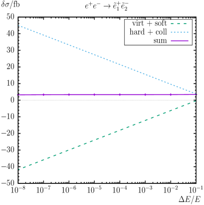
$\Delta E/E$	$\delta\sigma$/fbarn
$10^{-1}$	$3.460\pm 0.003$
$10^{-2}$	$3.365\pm 0.007$
$10^{-3}$	$3.358\pm 0.011$
$10^{-4}$	$3.359\pm 0.015$
$10^{-5}$	$3.361\pm 0.020$
$10^{-6}$	$3.342\pm 0.023$
$10^{-7}$	$3.299\pm 0.028$
$10^{-8}$	$3.231\pm 0.028$

Figure 2: Phase space slicing method. The different contributions to the one-loop corrections $\delta\sigma(e^{+}e^{-}\to\tilde{e}^{+}_{1}\tilde{e}^{-}_{2})$ for our input parameter scenario $\mathcal{S}$ (see Tab. 1 below) as a function of $\Delta E/E$ with fixed $\Delta\theta/\text{rad}=10^{-2}$.

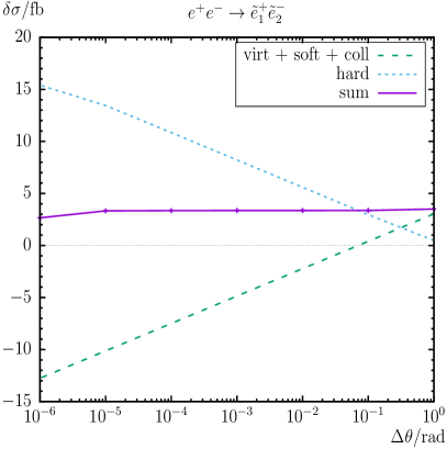
$\Delta\theta$/rad	$\delta\sigma$/fbarn
$10^{0}$	$3.503\pm 0.014$
$10^{-1}$	$3.362\pm 0.012$
$10^{-2}$	$3.358\pm 0.010$
$10^{-3}$	$3.356\pm 0.011$
$10^{-4}$	$3.352\pm 0.012$
$10^{-5}$	$3.329\pm 0.013$
$10^{-6}$	$2.653\pm 0.015$

Figure 3: Phase space slicing method. The different contributions to the one-loop corrections $\delta\sigma(e^{+}e^{-}\to\tilde{e}^{+}_{1}\tilde{e}^{-}_{2})$ for our input parameter scenario $\mathcal{S}$ (see Tab. 1 below) as a function of $\Delta\theta/\text{rad}$ with fixed $\Delta E/E=10^{-3}$.

In the phase space slicing method, the phase space is divided into regions where the integrand is finite (numerically stable) and regions where it is divergent (or numerically unstable). In the stable regions the integration is performed numerically, whereas in the unstable regions it is carried out (semi-) analytically using approximations for the collinear photon emission.

The collinear part is constrained by the angular cut-off parameter $\Delta\theta$, imposed on the angle between the photon and the (in our case initial state) electron/positron.

The differential cross section for the collinear photon radiation off the initial state $e^{+}e^{-}$ pair corresponds to a convolution

$$\text{d}\sigma_{\text{coll}}(s)=\frac{\alpha}{\pi}\int_{0}^{1-\delta_{s}}\text{d}z\,\text{d}\sigma_{\text{tree}}(\sqrt{zs})\left\{\left[2\,\ln\left(\frac{\Delta\theta\sqrt{s}}{2\,m_{e}}\right)-1\right]P_{ee}(z)+1-z\right\}\,,$$ (19)

with $P_{ee}(z)=(1+z^{2})/(1-z)$ denoting the splitting function of a photon from the initial $e^{+}e^{-}$ pair. The electron momentum is reduced (because of the radiated photon) by the fraction $z$ such that the center-of-mass frame of the hard process receives a boost. The integration over all possible factors $z$ is constrained by the soft cut-off $\delta_{s}=\Delta E/E$, to prevent over-counting in the soft energy region.

We have numerically checked that our results do not depend on the angular cut-off parameter $\Delta\theta$ over several orders of magnitude; see the example in Fig. 3. Our numerical results below have been obtained for fixed $\Delta\theta/\text{rad}=10^{-2}$.

The one-loop corrections of the differential cross section are decomposed into the virtual, soft, hard, and collinear parts as follows:

$$\text{d}\sigma_{\text{loop}}=\text{d}\sigma_{\text{virt}}(\lambda)+\text{d}\sigma_{\text{soft}}(\lambda,\Delta E)+\text{d}\sigma_{\text{hard}}(\Delta E,\Delta\theta)+\text{d}\sigma_{\text{coll}}(\Delta E,\Delta\theta)\,.$$ (20)

The hard and collinear parts have been calculated via Monte Carlo integration algorithms of the CUBA library [72, 73] as implemented in FormCalc [50, 51].

3 Comparisons

In this section we present the comparisons with results from other groups in the literature for slepton production in $e^{+}e^{-}$ collisions. These comparisons were restricted to the MSSM with real parameters, with one exception for tree-level tau slepton pair production. The level of agreement of such comparisons (at one-loop order) depends on the correct transformation of the input parameters from our renormalization scheme into the schemes used in the respective literature, as well as on the differences in the employed renormalization schemes as such. In view of the non-trivial conversions and the large number of comparisons such transformations and/or change of our renormalization prescription are beyond the scope of our paper. In the following we list all relevant papers in the literature and explain either our comparison, or why no (meaningful) comparison could be performed.

• In Ref. [34] the production of slepton and squark pairs in $e^{+}e^{-}$ annihilation and $Z$ decay have been calculated in the rMSSM at tree level (including arbitrarily polarized beams). Unfortunately, in Ref. [34] not sufficient information as regards their input parameters where given, rendering a comparison impossible.

• Selectron pair production at $e^{+}e^{-}$ colliders in SUGRA models were presented in Ref. [35] at tree level. We omitted a comparison with Ref. [35], since implementing the SUGRA spectrum is beyond the scope of our paper.

• Tree-level tau slepton pair production at muon colliders in the cMSSM were analyzed in Ref. [36] including ${\cal CP}$ violation. The center-of-mass energy was assumed to be around the resonances of the heavy neutral Higgs bosons, at $\sqrt{s}\simeq 500\,\,\mathrm{GeV}$. We used their input parameters as far as possible, but we differ from their results, especially in the case of complex input parameters. This can most likely be attributed to the differences in the Higgs-boson mass calculations employed in Ref. [36] and the current version 2.13.0 of FeynHiggs [60, 74, 75, 76, 77, 78, 79, 80], which we use. The cross section (close to the heavy Higgs boson thresholds) depends strongly on tiny mass differences of the two heavy neutral Higgs bosons, which deviate clearly between the two employed calculations, rendering this comparison not significant.

• In Refs. [37, 38] pair production of smuons and selectrons near threshold in $e^{+}e^{-}$ and $e^{-}e^{-}$ collisions have been computed in the rMSSM, including Coulomb rescattering effects. Because these near production threshold effects are beyond the scope of our paper we have omitted a comparison with Refs. [37, 38].

• Ref. [39] deals with selectron pair production at $e^{-}e^{-}$ and $e^{+}e^{-}$ colliders with polarized beams. The calculations have been computed in the rMSSM near the production threshold. Again, these effects are beyond the scope of our paper and we have omitted a comparison with Ref. [39].

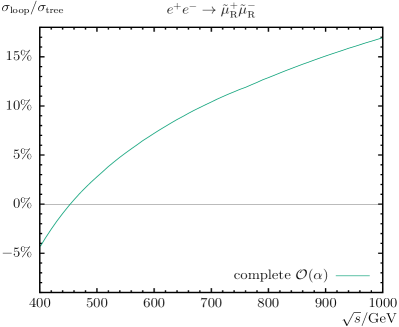
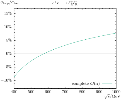
  Figure 4: Comparison with Ref. [40] for $e^{+}e^{-}\to{\tilde{e}_{s}}{\tilde{e}_{s^{\prime}}},{\tilde{\mu}_{s}}{\tilde{\mu}_{s^{\prime}}}$. Born cross sections (upper row) and complete relative one-loop results (lower row) are shown for the SPS$1a$ parameter point as given according to Ref. [40] as a function of $\sqrt{s}$.

• Also Ref. [40] is (mainly) based on Ref. [38]. The general production of scalar leptons at linear $e^{+}e^{-}$ colliders has been computed in Ref. [40], including multi-photon initial state radiation and polarized beams. The authors used (older versions of) FeynArts, FeynCalc [81] and LoopTools for their calculations. As input parameters they used the mSUGRA parameter point SPS$1a$ [82], translated from the $\smash{\overline{\mathrm{DR}}}$ to on-shell values; see the appendix of Ref. [40]. We also used this parameter point (as far as possible) and reproduced successfully their tree-level results in their Figs. 2 and 3a (see Ref. [40]) in the upper row of our Fig. 4. Our (relative) one-loop results are in qualitative agreement with the ones in their Figs. 17 and 18a of Ref. [40]; see the lower row in our Fig. 4. The quantitative numerical differences can be explained with the different renormalization schemes, slightly different input parameters, and the different treatment of the photon bremsstrahlung, where they have included multi-photon emission while we kept our calculation at ${\cal O}(\alpha)$. It should also be kept in mind that the relative one-loop corrections are sensitive to every kind of difference.

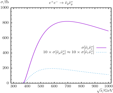
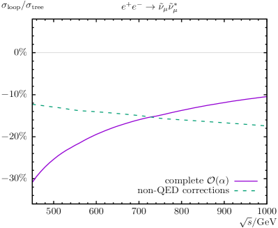
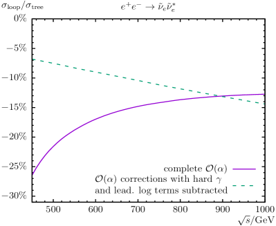
  Figure 5: Comparison with Ref. [41] for $e^{+}e^{-}\to\tilde{\nu}_{g}\tilde{\nu}_{g}^{*}$. Born cross sections (upper plot) and complete relative one-loop results (lower row) are shown for the SPS$1a$ parameter point as given according to Ref. [41] as a function of $\sqrt{s}$.

• Ref. [41] is an addendum to Ref. [40] dealing with $e^{+}e^{-}\to\tilde{\nu}_{g}\tilde{\nu}_{g}^{*}$. As input parameters they used the SUSY parameter point SPS$1a$ translated from the $\smash{\overline{\mathrm{DR}}}$ to on-shell values; see Ref. [82]. We reproduced successfully $e^{+}e^{-}\to\tilde{\nu}_{\mu}\tilde{\nu}_{\mu}^{*}$ and $e^{+}e^{-}\to\tilde{\nu}_{\tau}\tilde{\nu}_{\tau}^{*}$ of Ref. [41] in our Fig. 5. The (quantitative) difference in the relative loop corrections can be explained with the different renormalization schemes, slightly different input parameters, and the different treatment of the photon radiation, where they have included multi-photon emission while we kept our calculation at ${\cal O}(\alpha)$. The process $e^{+}e^{-}\to\tilde{\nu}_{e}\tilde{\nu}_{e}^{*}$, on the other hand, while in rather good qualitative agreement, differ quantitative significantly already at the tree level. Unfortunately, we were not able to trace back the source of the difference. However, since (in our automated approach) we agree with other tree-level calculations, we are confident that our results are correct.

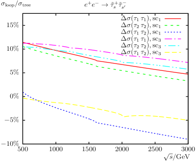
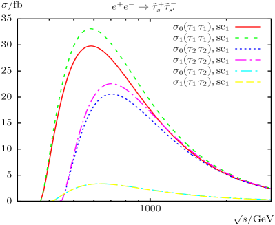
  Figure 6: Comparison with Ref. [42] for $\sigma(e^{+}e^{-}\to\tilde{\tau}^{+}_{s}\tilde{\tau}^{-}_{s^{\prime}})$. Total relative corrections (left) and tree-level and one-loop cross sections (right) as as functions of $\sqrt{s}$ are shown with scenarios sc₁ and sc₃ chosen according to Ref. [42].

• We performed a comparison with Ref. [42] using their input parameters (as far as possible). They have calculated (third generation) scalar fermion production in the rMSSM within an on-shell scheme close to ours at the “full” one-loop level (but without explicit QED radiation). They also used (older versions of) FeynTools for their calculations. We found very good agreement with their Fig. 13, as can be seen in our Fig. 6. The tiny differences can easily be explained with the slightly different SM input parameters and the slightly different renormalization scheme.

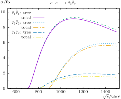
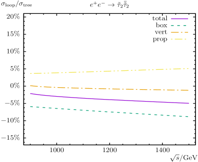
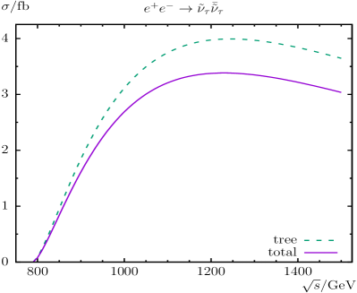
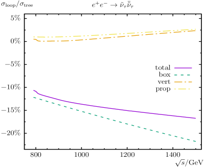
  Figure 7: Comparison with Ref. [43] for $\sigma(e^{+}e^{-}\to\tilde{\tau}^{+}_{s}\tilde{\tau}^{-}_{s^{\prime}})$ (upper row) and $\sigma(e^{+}e^{-}\to\tilde{\nu}_{\tau}\tilde{\nu}_{\tau}^{*})$ (lower row). The left (right) plot shows cross sections (relative corrections) with $\sqrt{s}$ varied within the Scenario 1 according to Ref. [43].

• In Refs. [43, 44] the “complete” one-loop corrections to $e^{+}e^{-}\to\tilde{f}_{s}\tilde{f}_{s^{\prime}}^{*}$ (third generation) in the rMSSM were analyzed numerically including photon corrections. However, their numerical results have been presented taking into account only weak corrections. They used (an older version of) LoopTools for their calculations and their own on-shell renormalization procedure together with a $\alpha(M_{Z})|_{\overline{\mathrm{MS}}}=1/127.934$ scheme. We used their “Scenario 1- gaugino” (as far as possible) for our comparison. We are in rather good agreement with their Figs. 4c, 4f, 7a, and 7d which can be seen in our Fig. 7. The minor differences can be explained (as usual) with the slightly different input parameters and the different renormalization scheme.

• Finally, in Refs. [44, 45] full ${\cal O}(\alpha)$ corrections to $e^{+}e^{-}\to\tilde{f}_{s}\tilde{f}_{s^{\prime}}^{*}$ have been calculated in the MSSM with real parameters. Polarized electrons and multi-photon bremsstrahlung were included in the phenomenological analysis. As input parameters they used the mSUGRA parameter point SPS$1a^{\prime}$ [82], translated from the $\smash{\overline{\mathrm{DR}}}$ to on-shell values. We also used this parameter point (as far as possible) and reproduced parts of their results in their Figs. 7 and 8 (see Ref. [45]) in our Fig. 8. We are in good agreement for the processes $e^{+}e^{-}\to\tilde{\tau}^{+}_{2}\tilde{\tau}^{-}_{2}$ and $e^{+}e^{-}\to\tilde{\tau}^{\pm}_{1}\tilde{\tau}^{\mp}_{2}$, while we disagree in $e^{+}e^{-}\to\tilde{\tau}^{+}_{1}\tilde{\tau}^{-}_{1}$ and $e^{+}e^{-}\to\tilde{\nu}_{\tau}\tilde{\nu}_{\tau}^{*}$ already at tree-level. Unfortunately, we were not able to track down the source of the differences. However, since we agree (in our automated approach) with other tree-level calculations, we are confident that our results are correct.

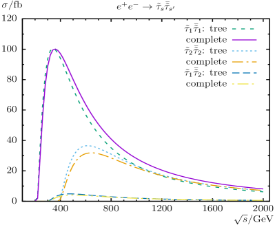
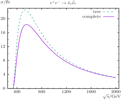
  Figure 8: Comparison with Ref. [45] for $\sigma(e^{+}e^{-}\to\tilde{\tau}^{+}_{s}\tilde{\tau}^{-}_{s^{\prime}})$ left plot and $\sigma(e^{+}e^{-}\to\tilde{\nu}_{\tau}\tilde{\nu}_{\tau}^{*})$ right plot. Tree and complete cross sections are shown within the parameter set SPS$1a^{\prime}$ chosen according to Ref. [45], varied with $\sqrt{s}$.

To conclude, in most cases where a meaningful comparison could be performed, we found good agreement with the literature where expected, and the encountered differences can be traced back to different renormalization schemes, corresponding mismatches in the input parameters and small differences in the SM parameters. Nevertheless, in some cases we disagree already significantly at tree-level but we were not able to track down the source of these differences. This does not disprove the reliability of our calculation because our computational method/code has already been successfully tested and compared with quite a few other programs; see Refs. [29, 52, 49, 53, 55, 56, 28, 30, 32]. After comparing with the existing literature we would like to stress again that here we present for the first time a full one-loop calculation of $\sigma(e^{+}e^{-}\to\mathrm{\tilde{e}}^{\pm}_{gs}\mathrm{\tilde{e}}^{\mp}_{gs^{\prime}})$ and $\sigma(e^{+}e^{-}\to\tilde{\nu}_{g}\tilde{\nu}_{g}^{*})$ in the cMSSM, using the scheme that was employed successfully already for the full one-loop decays of the (produced) sleptons. The various calculations can readily be used together for the full production and decay chain.

4 Numerical analysis

In this section we present our numerical analysis of slepton production at $e^{+}e^{-}$ colliders in the cMSSM. In the figures below we show the cross sections at the tree level (“tree”) and at the full one-loop level (“full”), which is the cross section including all one-loop corrections as described in Sect. 2. The CCN[1] renormalization scheme (i.e. OS conditions for the two charginos and the lightest neutralino) has been used for most evaluations. In cases where the CCN[1] scheme is divergent (i.e. $M_{2}=\mu$) and/or unreliable, also some CNN[$c,n,n^{\prime}$] schemes (OS conditions for one chargino and two neutralinos) have been used, as indicated below; see Ref. [49] for further informations to these renormalization schemes. It should be noted that within the CCN[1] scheme at $\mu=M_{2}$ a divergence already in the tree-level result can be induced by $\delta\mu$ through the shifted scalar lepton masses : $\delta\mu$ in Eq. (5a) enters via Eq. (6a) into Eq. (2.1) from which the slepton shifts are calculated. The divergence is suppressed with $m_{\mathrm{e}_{g}}$ (see Eq. (5a)). In several analyses in Sect. 4 in order to overcome the problem with a divergent tree-level result, we switched to the tree-level result of the CNN[1,2,3] scheme, which is free of such a divergence. When several schemes are shown in one plot, a full comparison would require the transition of the relevant input parameters (which are varied). However, we do not intend to perform an analysis of the advantages and disadvantages of the various renormalization schemes. We want to demonstrate, however, that it is always possible to choose a “good” renormalization scheme, i.e. a scheme that leads to stable and not excessively large higher-order corrections. Consequently, the above mentioned parameter conversion is not (yet) included in our calculation.

We first define the numerical scenario for the cross section evaluation. Then we start the numerical analysis with the cross sections of $e^{+}e^{-}\to\mathrm{\tilde{e}}^{\pm}_{gs}\mathrm{\tilde{e}}^{\mp}_{gs^{\prime}}$ ($g=1,2,3;\,s,s^{\prime}=1,2$) in Sect. 4.2, evaluated as a function of $\sqrt{s}$, $M_{\tilde{E}}$, $\mu$, $|M_{1}|$ and/or $M_{2}$, $\varphi_{A_{\mathrm{e}_{g}}}$ or $\varphi_{M_{1}}$, the phase of $M_{1}$. In some cases also the $t_{\beta}$ dependence is shown. Then we turn to the processes $e^{+}e^{-}\to\tilde{\nu}_{g}\tilde{\nu}_{g}^{*}$ in Sect. 4.3. All these processes are of particular interest for ILC and CLIC analyses [17, 18, 19, 20, 21, 23, 24] (as emphasized in Sect. 1).

4.1 Parameter settings

The renormalization scale $\mu_{R}$ has been set to the center-of-mass energy, $\sqrt{s}$. The SM parameters are chosen as follows; see also [83]:

• Fermion masses (on-shell masses, if not indicated differently):

  $$m_{e} =0.5109989461\,\,\mathrm{MeV}\,, m_{\nu_{e}} =0\,,$$

  $$m_{\mu} =105.6583745\,\,\mathrm{MeV}\,, m_{\nu_{\mu}} =0\,,$$

  $$m_{\tau} =1776.86\,\,\mathrm{MeV}\,, m_{\nu_{\tau}} =0\,,$$

  $$m_{u} =70.59\,\,\mathrm{MeV}\,, m_{d} =70.59\,\,\mathrm{MeV}\,,$$

  $$m_{c} =1.280\,\,\mathrm{GeV}\,, m_{s} =96.00\,\,\mathrm{MeV}\,,$$

  $$m_{t} =173.1\,\,\mathrm{GeV}\,, m_{b} =2.954\,\,\mathrm{GeV}\,.$$ (21)

  According to Ref. [83], $m_{s}$ is an estimate of a so-called ”current quark mass” in the $\overline{\mathrm{MS}}$ scheme at the scale $\mu\approx 2\,\,\mathrm{GeV}$. $m_{c}\equiv m_{c}(m_{c})$ is the ”running” mass in the $\overline{\mathrm{MS}}$ scheme and $m_{b}\equiv m^{\smash{\overline{\mathrm{DR}}}}_{b}$ is the $\smash{\overline{\mathrm{DR}}}$ bottom quark mass as calculated in Ref. [55]. $m_{u}$ and $m_{d}$ are effective parameters, calculated through the hadronic contributions to

  $$\Delta\alpha_{\text{had}}^{(5)}(M_{Z}) =\frac{\alpha}{\pi}\sum_{f=u,c,d,s,b}Q_{f}^{2}\Bigl{(}\ln\frac{M_{Z}^{2}}{m_{f}^{2}}-\frac{5}{3}\Bigr{)}\approx 0.02764\,.$$ (22)

• Gauge-boson masses:

  $$M_{Z}=91.1876\,\,\mathrm{GeV}\,,\qquad M_{W}=80.385\,\,\mathrm{GeV}\,.$$ (23)

• Coupling constant:

  $$\alpha(0)=1/137.035999139\,.$$ (24)

The SUSY parameters are chosen according to the scenario $\mathcal{S}$, shown in Tab. 1. This scenario is viable for the various cMSSM slepton production modes, i.e. not picking specific parameters for each cross section. They are in particular in agreement with the relevant SUSY searches of ATLAS and CMS: Our electroweak spectrum is not covered by the latest ATLAS/CMS exclusion bounds. Two limits have to be distinguished. The limits not taking into account a possible intermediate slepton exclude a lightest neutralino only well below $300\,\,\mathrm{GeV}$ [84, 85], whereas in $\mathcal{S}$ we have $m_{\tilde{\chi}_{1}^{0}}\approx 323\,\,\mathrm{GeV}$. Limits with intermediary sleptons often assume a chargino decay to lepton and sneutrino, while in our scenario $m_{\tilde{\chi}_{1}^{\pm}}<m_{\tilde{\nu}_{e,\mu,\tau}}$. Furthermore, the exclusion bounds given in the $m_{\tilde{\chi}_{1}^{0}}$-$m_{\tilde{\chi}_{2}^{0}}$ mass plane (with $m_{\tilde{\chi}_{2}^{0}}\approx m_{\tilde{\chi}_{1}^{\pm}}$ assumed) above $m_{\tilde{\chi}_{2}^{0}}\sim 300\,\,\mathrm{GeV}$ do not cover a compressed spectrum [84, 86] for $\tilde{\chi}_{1}^{0}$, $\tilde{\chi}_{2}^{0}$, and $\tilde{\chi}_{1}^{\pm}$. In particular our scenario $\mathcal{S}$ assumed masses of $m_{\tilde{\chi}_{1}^{0}}\approx 323\,\,\mathrm{GeV}$ and $m_{\tilde{\chi}_{2}^{0}}\approx 354\,\,\mathrm{GeV}$, which are not excluded.

Table 1: MSSM default parameters for the numerical investigation; all parameters (except of $t_{\beta}$) are in GeV. The values for the trilinear sfermion Higgs couplings, $A_{f}$ are chosen to be real (except for $A_{\mathrm{e}_{g}}$ which can be complex) and such that charge- and/or color-breaking minima are avoided [87, 88, 89, 90, 91, 92, 93]. It should be noted that we chose common values $M_{\tilde{Q},\tilde{U},\tilde{D}}=2000\,\,\mathrm{GeV}$ for all squark generations, and $M_{\tilde{L}}=M_{\tilde{E}}+50\,\,\mathrm{GeV}$ for all slepton generations. For the sleptons we show the tree-level values as well as their OS masses in our DR[2] renormalization scheme; see Sect. 2.1.

Scen.	$\sqrt{s}$	$t_{\beta}$	$\mu$	$M_{H^{\pm}}$	$M_{\tilde{Q},\tilde{U},\tilde{D}}$	$M_{\tilde{E}}$	$A_{\mathrm{u}_{g}}$	$A_{\mathrm{d}_{g}}$	$|A_{\mathrm{e}_{g}}|$	$|M_{1}|$	$M_{2}$	$M_{3}$
$\mathcal{S}$	1000	10	350	1200	2000	300	2600	2000	2000	400	600	2000

	$m_{\tilde{\nu}_{e,\mu,\tau}}$	$m_{\tilde{e}_{1}}$	$m_{\tilde{e}_{2}}$	$m_{\tilde{\mu}_{1}}$	$m_{\tilde{\mu}_{2}}$	$m_{\tilde{\tau}_{1}}$	$m_{\tilde{\tau}_{2}}$
tree	344.129	303.013	353.212	303.012	353.213	302.664	353.519
OS	344.129	303.013	352.973	303.012	352.974	302.664	353.264

It should be noted that higher-order corrected Higgs-boson masses do not enter our calculation. However, we ensured that over larger parts of the parameter space the lightest Higgs-boson mass is around $\sim 125\pm 3\,\,\mathrm{GeV}$ to indicate the phenomenological validity of our scenarios. In our numerical evaluation we will show the variation with $\sqrt{s}$ (up to $3\,\,\mathrm{TeV}$, shown in the upper left plot of the respective figures), $M_{\tilde{E}}$ (from 100 to 500 GeV, upper right plot), $\mu$ (starting at $\mu=100\,\,\mathrm{GeV}$ up to $\mu=1000\,\,\mathrm{GeV}$, shown in the middle/lower left plots), $|M_{1}|$ or $M_{2}$ (from 100 to 1000 GeV, middle/lower right plots), and $\varphi_{A_{\mathrm{e}_{g}}}$ or $\varphi_{M_{1}}$ (between $0^{\circ}$ and $360^{\circ}$, lower right plots). The dependence of $t_{\beta}$ turned out to be rather small, therefore we show it only in a few cases, where it is of special interest.

Concerning the complex parameters, some more comments are in order. Potentially complex parameters that enter the selectron and electron sneutrino production cross sections at tree level (via the $t$-channel exchange of a neutralino or chargino) are the soft SUSY-breaking parameters $M_{1}$ and $M_{2}$ as well as the Higgs mixing parameter $\mu$. Also trilinear slepton couplings $A_{\mathrm{e}_{g}}$ enter the tree-level production cross sections. However, when performing an analysis involving complex parameters it should be noted that the results for physical observables are affected only by certain combinations of the complex phases of the parameters $\mu$, the trilinear couplings $A_{f}$ and the gaugino mass parameters $M_{1,2,3}$ [95, 96]. It is possible, for instance, to rotate the phase $\varphi_{M_{2}}$ away. Experimental constraints on the (combinations of) complex phases arise, in particular, from their contributions to electric dipole moments of the electron and the neutron (see Refs. [97, 98, 99] and the references therein), of the deuteron [100] and of heavy quarks [101, 102]. While SM contributions enter only at the three-loop level, due to its complex phases the MSSM can contribute already at one-loop order. Large phases in the first two generations of sfermions can only be accommodated if these generations are assumed to be very heavy [103, 104] or large cancellations occur [105, 106, 107]; see, however, the discussion in Ref. [108]. A review can be found in Ref. [109]. Recently additional constraints at the two-loop level on some ${\cal CP}$ phases of SUSY models have been investigated in Ref. [110]. Accordingly (using the convention that $\varphi_{M_{2}}=0$, as done in this paper), in particular, the phase $\varphi_{\mu}$ is tightly constrained [111], and we set it to zero. On the other hand, the bounds on the phases of the third-generation trilinear couplings are much weaker. Consequently, the largest effects on the slepton production cross sections at the tree level are expected from the complex gaugino mass parameter $M_{1}$, i.e. from $\varphi_{M_{1}}$. As mentioned above, the only other phase entering at the tree level, is $\varphi_{A_{\mathrm{e}_{g}}}$. This motivates our choice of $\varphi_{M_{1}}$ and $\varphi_{A_{\mathrm{e}_{g}}}$ as parameters to be varied.

Since now complex parameters can appear in the couplings, contributions from absorptive parts of self-energy type corrections on external legs can arise. The corresponding formulas for an inclusion of these absorptive contributions via finite wave function correction factors can be found in Refs. [49, 55].

The numerical results shown in the next subsections are of course dependent on the choice of the SUSY parameters. Nevertheless, they give an idea of the relevance of the full one-loop corrections.

4.2 The process $e^{+}e^{-}\to\mathrm{\tilde{e}}^{\pm}_{gs}\mathrm{\tilde{e}}^{\mp}_{gs^{\prime}}$

In Figs. 9 – 17 we show the results for the processes $e^{+}e^{-}\to\mathrm{\tilde{e}}^{\pm}_{gs}\mathrm{\tilde{e}}^{\mp}_{gs^{\prime}}$ ($g=1,2,3;\,s,s^{\prime}=1,2$) as a function of $\sqrt{s}$, $M_{\tilde{E}}$, $\mu$, $|M_{1}|$, $M_{2}$, $t_{\beta}$, $\varphi_{M_{1}}$, and $\varphi_{A_{\mathrm{e}_{g}}}$. It should be noted that for $s\to\infty$ decreasing cross sections $\propto\ln{(s)}/s$ for the first and $\propto 1/s$ for the second and third slepton generations are expected; see Ref. [40]. We also remind the reader that $\sigma(e^{+}e^{-}\to\mathrm{\tilde{e}}^{\pm}_{gs}\mathrm{\tilde{e}}^{\mp}_{gs^{\prime}})$ denotes the sum of the two charge conjugated processes $\forall\;s\neq s^{\prime}$; see Eq. (18).

We start with the process $e^{+}e^{-}\to\tilde{e}^{+}_{1}\tilde{e}^{-}_{1}$ shown in Fig. 9. Away from the production threshold, loop corrections of $\sim+6\,\%$ at $\sqrt{s}=1000\,\,\mathrm{GeV}$ are found in scenario $\mathcal{S}$ (see Tab. 1), with a maximum of $27\,\mbox{fb}$ at $\sqrt{s}\approx 1700\,\,\mathrm{GeV}$. The relative size of the loop corrections increase with increasing $\sqrt{s}$ and reach $\sim+21\,\%$ at $\sqrt{s}=3000\,\,\mathrm{GeV}$. A “tree crossing” (i.e. where the loop corrections become zero and therefore cross the tree-level result) can be found at $\sqrt{s}\approx 825\,\,\mathrm{GeV}$.

The cross sections are decreasing with increasing $M_{\tilde{E}}$ due to kinematics, and the full one-loop result has its maximum of $\sim 28\,\mbox{fb}$ at $M_{\tilde{E}}=100\,\,\mathrm{GeV}$. Analogously the relative corrections are decreasing from $\sim+13\,\%$ at $M_{\tilde{E}}=100\,\,\mathrm{GeV}$ to $\sim-30\%$ at $M_{\tilde{E}}=490\,\,\mathrm{GeV}$. The tree crossing takes place at $M_{\tilde{E}}\approx 375\,\,\mathrm{GeV}$. For higher $M_{\tilde{E}}$ values the loop corrections are negative, where the relative size becomes large due to the (relative) smallness of the tree-level results, which goes to zero for $M_{\tilde{E}}\approx 500\,\,\mathrm{GeV}$ due to kinematics. For the other parameter variations one can conclude that a cross section roughly twice as large can be possible for very low $M_{\tilde{E}}$ (which, however, are challenged by the current ATLAS/CMS exclusion bounds).

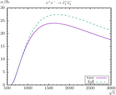
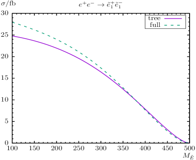
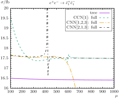
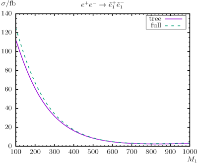
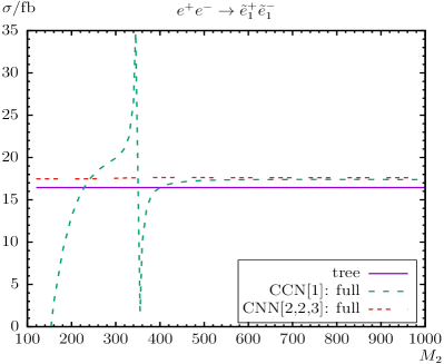
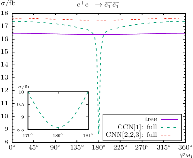
Figure 9: $\sigma(e^{+}e^{-}\to\tilde{e}^{+}_{1}\tilde{e}^{-}_{1})$. Tree-level and full one-loop corrected cross sections are shown with parameters chosen according to $\mathcal{S}$; see Tab. 1. The upper plots show the cross sections with $\sqrt{s}$ (left) and $M_{\tilde{E}}$ (right) varied; the middle plots show $\mu$ (left) and $|M_{1}|$ (right) varied; the lower plots show $M_{2}$ (left) and $\varphi_{M_{1}}$ (right) varied. All masses and energies are in GeV.

With increasing $\mu$ in $\mathcal{S}$ (middle left plot) we find a decrease of the loop corrected production cross section within CCN[1] (green dashed line). The relative loop corrections reach $\sim+18\,\%$ at $\mu=100\,\,\mathrm{GeV}$ (at the border of the experimental exclusion bounds) and $\sim+7\,\%$ at $\mu=600$-$1000\,\,\mathrm{GeV}$. One can see the expected breakdown of the CCN[1] scheme for $\mu=M_{2}$, i.e. in our case at $\mu\approx M_{2}=600\,\,\mathrm{GeV}$ (see also Refs. [32, 33]). Therefore, in the middle left plot of Fig. 9 also the corresponding results are shown for the CNN[1,2,3] (yellow dash-dotted line) and CNN[2,1,3] (black dash-dotted line) schemes, which are smooth at $\mu=M_{2}$. Outside the region of $\mu\sim M_{2}$ the scheme CCN[1] is expected to be reliable, since each of the three OS conditions is strongly connected to one of the three input parameters, $|M_{1}|$, $M_{2}$ and $\mu$. Similarly, CNN[1,2,3] is expected to be reliable for $\mu$ smaller than $M_{2}$, as in this case, again each of the three OS renormalization conditions is strongly connected to the three input parameters. This behavior can be observed in the plot: for $\mu\;\raisebox{-3.00003pt}{$\stackrel{{\scriptstyle\displaystyle<}}{{\sim}}$}\;M_{2}=600\,\,\mathrm{GeV}$ CNN[1,2,3] is reliable, while for $\mu\;\raisebox{-3.00003pt}{$\stackrel{{\scriptstyle\displaystyle>}}{{\sim}}$}\;M_{2}=600\,\,\mathrm{GeV}$ it becomes unreliable. While $\delta\mu$ in the CNN[2,1,3] scheme has a strong minimum at $\mu\approx 421\,\,\mathrm{GeV}$, dominating the loop corrections, it approximates CCN[1] very good for $\mu\;\raisebox{-3.00003pt}{$\stackrel{{\scriptstyle\displaystyle>}}{{\sim}}$}\;500\,\,\mathrm{GeV}$. A rising deviation between the schemes can be observed for $\mu<250\,\,\mathrm{GeV}$, where the schemes CNN[1,2,3] and CNN[2,1,3] are nearly constant, i.e. independent of $\mu$. Overall, it is possible to find for every value of $\mu$ a renormalization scheme that behaves stable and “flat” w.r.t. the tree-level cross section.

With increasing $|M_{1}|$ in $\mathcal{S}$ (middle right plot) we find a strong decrease of the production cross section, due to the change in the interference of the $\tilde{\chi}_{1}^{0}$ (dominant for $|M_{1}|\;\raisebox{-3.00003pt}{$\stackrel{{\scriptstyle\displaystyle<}}{{\sim}}$}\;340\,\,\mathrm{GeV}$), $\tilde{\chi}_{3}^{0}$ (dominant for $340\,\,\mathrm{GeV}\;\raisebox{-3.00003pt}{$\stackrel{{\scriptstyle\displaystyle<}}{{\sim}}$}\;|M_{1}|\;\raisebox{-3.00003pt}{$\stackrel{{\scriptstyle\displaystyle<}}{{\sim}}$}\;610\,\,\mathrm{GeV}$), and $\tilde{\chi}_{4}^{0}$ (dominant for $|M_{1}|\;\raisebox{-3.00003pt}{$\stackrel{{\scriptstyle\displaystyle>}}{{\sim}}$}\;610\,\,\mathrm{GeV}$) in the $t$-channel. It should be noted that there is no tree crossing in this plot. The loop corrections decrease from $\sim+11\%$ at $|M_{1}|=100\,\,\mathrm{GeV}$ to $\sim+3.8\%$ at $|M_{1}|=530\,\,\mathrm{GeV}$ and then increase to $\sim+15\%$ at $|M_{1}|=920\,\,\mathrm{GeV}$. However, for $|M_{1}|\;\raisebox{-3.00003pt}{$\stackrel{{\scriptstyle\displaystyle>}}{{\sim}}$}\;700\,\,\mathrm{GeV}$ the production cross section becomes relatively small.

The dependence $M_{2}$ of the cross section in $\mathcal{S}$ is shown in the lower left plot. One can clearly see the expected breakdown of the CCN[1] scheme for $M_{2}=\mu$, i.e. in our case at $M_{2}\approx\mu=350\,\,\mathrm{GeV}$ (see also Refs. [32, 33]) and the smooth behavior of CNN[2,2,3] (red dashed line) around $M_{2}\sim\mu=350\,\,\mathrm{GeV}$. Within CCN[1] the cross section even turns out to be negative for $M_{2}<154\,\,\mathrm{GeV}$ due to a maximum of $\delta M_{1}$ at $M_{2}\approx 20\,\,\mathrm{GeV}$, dominating the loop corrections. This renders the CCN[1] scheme to be unreliable for $M_{2}\;\raisebox{-3.00003pt}{$\stackrel{{\scriptstyle\displaystyle<}}{{\sim}}$}\;\mu$. For $M_{2}\;\raisebox{-3.00003pt}{$\stackrel{{\scriptstyle\displaystyle>}}{{\sim}}$}\;\mu$, on the other hand, the scheme CCN[1] is expected to be reliable, since each of the three OS conditions is strongly connected to one of the three input parameters, $|M_{1}|$, $M_{2}$ and $\mu$. The loop corrections at the level of $\sim+6\,\%$ are found to be nearly independent of $M_{2}$ for $M_{2}\;\raisebox{-3.00003pt}{$\stackrel{{\scriptstyle\displaystyle>}}{{\sim}}$}\;\mu$ within the CCN[1] scheme. And corrections of $\sim+7\,\%$ are found to be (nearly) independent of $M_{2}$ within the CNN[2,2,3] scheme.

Now we turn to the complex phase dependence. We find that the phase dependence $\varphi_{M_{1}}$ of the cross section in $\mathcal{S}$ is large for CCN[1] (lower right plot, green dashed line). Loop corrections at the level of $\sim+6\,\%$ at $\varphi_{M_{1}}=0^{\circ},360^{\circ}$ and $\sim-48\,\%$ at $\varphi_{M_{1}}=180^{\circ}$ are found. It should be noted here, that there is no divergency or threshold at $\varphi_{M_{1}}=180^{\circ}$, the cross section is smooth/finite; see the inlay in the lower right plot. This large structure is caused by a strong (local) minimum of the renormalization constant $\delta M_{1}$ at $\varphi_{M_{1}}=180^{\circ}$, dominating the loop corrections. Using another renormalization scheme (e.g. CNN[2,2,3]) the dip disappears, as can be seen in the plot. The one-loop corrections then reach $\sim+7\,\%$ and are nearly independent from $\varphi_{M_{1}}$. The loop effects of $\varphi_{A_{\mathrm{e}_{g}}}$, on the other hand, are tiny and therefore not shown explicitely.

The relative corrections for the process $e^{+}e^{-}\to\tilde{e}^{\pm}_{1}\tilde{e}^{\mp}_{2}$, as shown in Fig. 10, are rather large for the parameter set chosen; see Tab. 1. In the upper left plot of Fig. 10 the relative corrections grow from $\sim+16.6\,\%$ at $\sqrt{s}\approx 1000\,\,\mathrm{GeV}$ (i.e. $\mathcal{S}$) up to $\sim+35\,\%$ at $\sqrt{s}\approx 3000\,\,\mathrm{GeV}$. The tree crossing takes place at $\sqrt{s}\approx 730\,\,\mathrm{GeV}$ (where the higher-order corrections are relatively small around the crossing) and the maximum cross section of $52\,\mbox{fb}$ is reached at $\sqrt{s}\approx 850\,\,\mathrm{GeV}$.

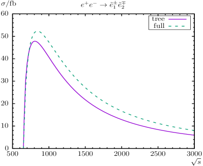
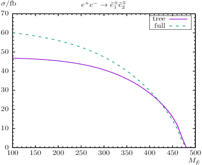
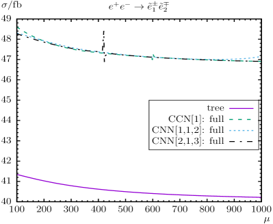
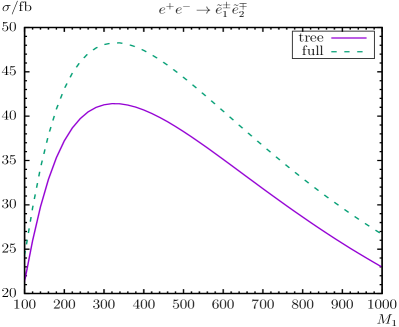
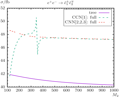
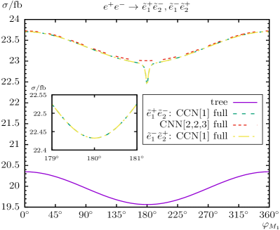
Figure 10: $\sigma(e^{+}e^{-}\to\tilde{e}^{\pm}_{1}\tilde{e}^{\mp}_{2})$. Tree-level and full one-loop corrected cross sections are shown with parameters chosen according to $\mathcal{S}$; see Tab. 1. The upper plots show the cross sections with $\sqrt{s}$ (left) and $M_{\tilde{E}}$ (right) varied; the middle plots show $\mu$ (left) and $|M_{1}|$ (right) varied; the lower plots show $M_{2}$ (left) and $\varphi_{M_{1}}$ (right) varied. All masses and energies are in GeV.

The dependence on $M_{\tilde{E}}$ is shown in the upper right plot of Fig. 10 and follows the same pattern as for $e^{+}e^{-}\to\tilde{e}^{+}_{1}\tilde{e}^{-}_{1}$, i.e. a strong decrease with increasing $M_{\tilde{E}}$ as obvious from kinematics. The loop corrections decrease from $\sim+28\%$ at $M_{\tilde{E}}=100\,\,\mathrm{GeV}$ to $\sim-31\%$ at $M_{\tilde{E}}=470\,\,\mathrm{GeV}$ (the latter is due to the smallness of the tree-level cross section), with a tree crossing at $M_{\tilde{E}}=425\,\,\mathrm{GeV}$.

The Higgs mixing parameter $\mu$ dependence is shown in the middle left plot. It is rather linear and decreasing from $\sim 48.6\,\mbox{fb}$ at small $\mu$ down to $\sim 46.9\,\mbox{fb}$ at $\mu=1000\,\,\mathrm{GeV}$. The relative corrections are $\sim+17.5\,\%$ at $\mu=100\,\,\mathrm{GeV}$ and $\sim 16.6\,\%$ at $\mu=1000\,\,\mathrm{GeV}$. In this case the (expected) breakdown of the CCN[1] scheme for $\mu\approx M_{2}=600\,\,\mathrm{GeV}$ is rather weakly pronounced. The corresponding results are shown for the CNN[1,1,2] and CNN[2,1,3] schemes, which are smooth at $\mu=M_{2}$. For small and large values of $\mu$ CNN[1,1,2] differs from CCN[1], whereas the other scheme, CNN[2,1,3], is very close to CCN[1]. While the CNN[2,1,3] scheme has a strong (local) minimum of $\delta\mu$ at $\mu\approx 421\,\,\mathrm{GeV}$, dominating the loop corrections, it approximates CCN[1] rather good for all other values of $\mu$.

The dependence on $|M_{1}|$ is shown in the middle right plot of Fig. 10. A strong dependence of the tree-level cross section can be observed (from the dominant neutralino $t$-channel exchange), which is amplified at the one-loop level. The size of the loop corrections varies from $\sim+16.6\%$ at $|M_{1}|=350\,\,\mathrm{GeV}$ (i.e. $\mathcal{S}$) to $\sim+15.2\%$ at $|M_{1}|=750\,\,\mathrm{GeV}$ and then increase again to $\sim+16.1\%$ at $|M_{1}|=1000\,\,\mathrm{GeV}$.

The cross section dependence of $M_{2}$ in $\mathcal{S}$ is shown in the lower left plot. Again, one can see the (expected) breakdown of the CCN[1] scheme for $M_{2}\approx\mu=350\,\,\mathrm{GeV}$ and the smooth behavior of CNN[2,2,3] around $M_{2}\approx\mu=350\,\,\mathrm{GeV}$. For $M_{2}\;\raisebox{-3.00003pt}{$\stackrel{{\scriptstyle\displaystyle>}}{{\sim}}$}\;\mu$ the scheme CCN[1] is expected to be reliable, while CNN[2,2,3] is reliable for all values of $M_{2}$; see above. The combined (reliable) one-loop corrections of CCN[1] and CNN[2,2,3] at the level of $\sim+16\,\%$ are found to be only weakly dependent of $M_{2}$.

The phase dependence $\varphi_{M_{1}}$ of the cross section in $\mathcal{S}$ is shown in the lower right plot of Fig. 10. In this case it turns out to be substantial, already changing the tree-level cross section by up to $3.7\,\%$. The relative loop corrections ($\sigma_{\text{loop}}/\sigma_{\text{tree}}$) vary with $\varphi_{M_{1}}$ between $\sim+14.6\,\%$ at $\varphi_{M_{1}}=180^{\circ}$ and $\sim+17.3\,\%$ at $\varphi_{M_{1}}=158^{\circ},203^{\circ}$ for CCN[1]. Again, the cross section does not diverge at $\varphi_{M_{1}}=180^{\circ}$. This structure is caused by a minimum of $\delta M_{1}$ at $\varphi_{M_{1}}=180^{\circ}$, dominating the loop corrections. Using the CNN[2,2,3] scheme (red dashed line) the dip disappears, as can be seen in the plot. The relative loop corrections reach $\sim+17.7\,\%$ at $\varphi_{M_{1}}=180^{\circ}$. For our parameter set $\mathcal{S}$, with the complex phase $\varphi_{M_{1}}$, the ${\cal CP}$ asymmetry turn out to be (numerically) zero, which can be seen from the identical green dashed ($\tilde{e}^{+}_{1}\tilde{e}^{-}_{2}$) and yellow dash-dotted ($\tilde{e}^{-}_{1}\tilde{e}^{+}_{2}$) lines. Finally the variation with $\varphi_{A_{\mathrm{e}_{g}}}$ is again negligible and not shown here.

We now turn to the process $e^{+}e^{-}\to\tilde{e}^{+}_{2}\tilde{e}^{-}_{2}$ shown in Fig. 11, which is found to be of ${\cal O}(10\,\mbox{fb})$. As a function of $\sqrt{s}$ (upper left plot) the loop corrections range from $\sim-3\,\%$ at $\sqrt{s}=1000\,\,\mathrm{GeV}$ (i.e. $\mathcal{S}$) to $\sim-10\,\%$ at $\sqrt{s}=3000\,\,\mathrm{GeV}$.

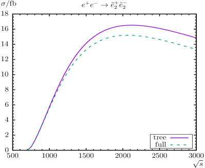
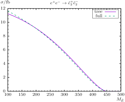
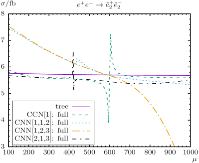
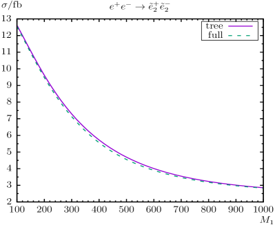
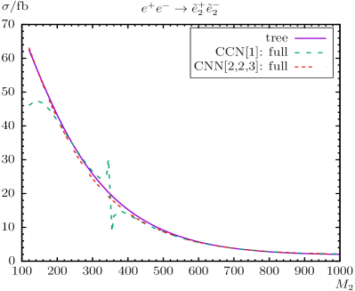
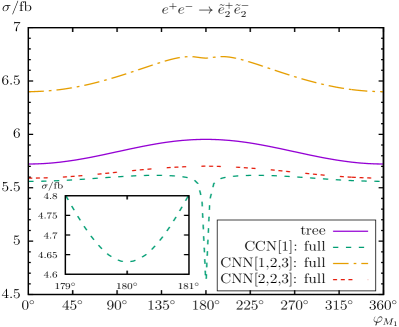
Figure 11: $\sigma(e^{+}e^{-}\to\tilde{e}^{+}_{2}\tilde{e}^{-}_{2})$. Tree-level and full one-loop corrected cross sections are shown with parameters chosen according to $\mathcal{S}$; see Tab. 1. The upper plots show the cross sections with $\sqrt{s}$ (left) and $M_{\tilde{E}}$ (right) varied; the middle plots show $\mu$ (left) and $|M_{1}|$ (right) varied; the lower plots show $M_{2}$ (left) and $\varphi_{M_{1}}$ (right) varied. All masses and energies are in GeV.

The cross sections are decreasing with increasing $M_{\tilde{E}}$ due to kinematics, and the full one-loop result has its maximum of $\sim 11.6\,\mbox{fb}$ at $M_{\tilde{E}}=100\,\,\mathrm{GeV}$. Analogously the relative corrections are decreasing from $\sim+4\,\%$ at $M_{\tilde{E}}=100\,\,\mathrm{GeV}$ to $\sim-23\%$ at $M_{\tilde{E}}=440\,\,\mathrm{GeV}$. The tree crossing takes place at $M_{\tilde{E}}\approx 190\,\,\mathrm{GeV}$. For higher $M_{\tilde{E}}$ values the loop corrections are negative, where the relative size becomes large due to the (relative) smallness of the tree-level results, which goes to zero for $M_{\tilde{E}}\approx 450\,\,\mathrm{GeV}$ due to kinematics. For the other parameter variations one can conclude that a cross section twice as large can be possible for very low $M_{\tilde{E}}$ (which however are challenged by the current ATLAS/CMS exclusion bounds).

The dependence on $\mu$ (middle left plot) is rather small. The one-loop corrections within the CCN[1] scheme are $\sim+2\,\%$ at $\mu=100\,\,\mathrm{GeV}$, $\sim-2\,\%$ at $\mu=1000\,\,\mathrm{GeV}$ and have a tree crossing at $\mu\approx 150\,\,\mathrm{GeV}$. The corresponding smooth results CNN[1,1,2] and CNN[1,2,3] are shown, but both differ for small values (and CNN[1,2,3] also for large values) of $\mu$ significantly from CCN[1]. Therefore, in addition we also show the CNN[2,1,3] scheme (black dash-dotted line) which approximates CCN[1] very good for all values of $\mu$ except for $\mu\approx 421\,\,\mathrm{GeV}$ where $\delta\mu$ has a strong (local) minimum, that dominates the loop corrections in this part of the parameter space.

With increasing $|M_{1}|$ in $\mathcal{S}$ (middle right plot) we find again a strong decrease of the production cross section, due to the change in the interference of the (dominant) neutralinos in the $t$-channel. It should be noted that there is no tree crossing in this plot. The loop corrections are rather small and decrease from $\sim-0.6\%$ at $|M_{1}|=100\,\,\mathrm{GeV}$ to $\sim-3\%$ at $|M_{1}|=470\,\,\mathrm{GeV}$ and then increase to $\sim-0.9\%$ at $|M_{1}|=1000\,\,\mathrm{GeV}$.

The dependence $M_{2}$ of the cross section in $\mathcal{S}$ is shown in the lower left plot of Fig. 11. The tree cross section decreases strongly from $\sim 62\,\mbox{fb}$ at $M_{2}=120\,\,\mathrm{GeV}$ down to $\sim 2\,\mbox{fb}$ at $M_{2}=1000\,\,\mathrm{GeV}$, because of the change in the interference of the $\tilde{\chi}_{1}^{0}$ (dominant for $M_{2}\;\raisebox{-3.00003pt}{$\stackrel{{\scriptstyle\displaystyle<}}{{\sim}}$}\;300\,\,\mathrm{GeV}$), $\tilde{\chi}_{3}^{0}$ (dominant for $300\,\,\mathrm{GeV}\;\raisebox{-3.00003pt}{$\stackrel{{\scriptstyle\displaystyle<}}{{\sim}}$}\;M_{2}\;\raisebox{-3.00003pt}{$\stackrel{{\scriptstyle\displaystyle<}}{{\sim}}$}\;480\,\,\mathrm{GeV}$), and $\tilde{\chi}_{4}^{0}$ (dominant for $M_{2}\;\raisebox{-3.00003pt}{$\stackrel{{\scriptstyle\displaystyle>}}{{\sim}}$}\;480\,\,\mathrm{GeV}$) in the $t$-channel. As before, one can see the breakdown of the CCN[1] scheme for $M_{2}\approx\mu=350$, and the smooth behavior of CNN[2,2,3] (red dashed line) around $M_{2}\approx\mu=350\,\,\mathrm{GeV}$. Again, CCN[1] is reliable for $M_{2}\;\raisebox{-3.00003pt}{$\stackrel{{\scriptstyle\displaystyle>}}{{\sim}}$}\;400\,\,\mathrm{GeV}$ while CNN[2,2,3] is reliable for all values of $M_{2}$ and very close to CCN[1]. The (reliable) one-loop corrections of CCN[1] and CNN[2,2,3] are at the level of $\sim\pm 5\,\%$. The CNN[1,2,3] scheme (not shown) is also smooth for all values of $M_{2}$ and can reach $\sim+20\,\%$ at $M_{2}\approx 800\,\,\mathrm{GeV}$.

Now we turn to the complex phase dependence. We find that the phase dependence $\varphi_{M_{1}}$ of the cross section in $\mathcal{S}$ is rather large (lower right plot) for the CCN[1] scheme. Loop corrections at the level of $\sim-3\,\%$ at $\varphi_{M_{1}}=0^{\circ},360^{\circ}$ and $\sim-22\,\%$ at $\varphi_{M_{1}}=180^{\circ}$ are found. It should be noted again, that there is no divergency or threshold at $\varphi_{M_{1}}=180^{\circ}$, the cross section does not diverge; see the inlay in the lower right plot. This large structure is caused by a strong minimum of $\delta M_{1}$ at $\varphi_{M_{1}}=180^{\circ}$, dominating the loop corrections. The CNN[2,2,3] scheme (red dashed line) is close to CCN[1] at the level of $\sim-3\,\%$ without this peculiar structure. In contrast the full corrections of CNN[1,2,3] reach $\sim+13\,\%$. The loop effects of $\varphi_{A_{\mathrm{e}_{g}}}$, on the other hand, are tiny and therefore not shown explicitely.

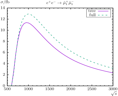
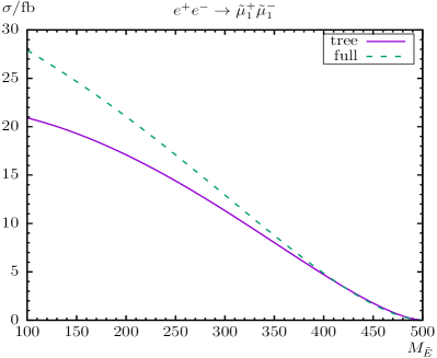
Figure 12: $\sigma(e^{+}e^{-}\to\tilde{\mu}^{+}_{1}\tilde{\mu}^{-}_{1})$. Tree-level and full one-loop corrected cross sections are shown with parameters chosen according to $\mathcal{S}$; see Tab. 1. The plots show the cross sections with $\sqrt{s}$ (left) and $M_{\tilde{E}}$ (right) varied. All masses and energies are in GeV.

We now turn to the second generation charged slepton production. The process $e^{+}e^{-}\to\tilde{\mu}^{+}_{1}\tilde{\mu}^{-}_{1}$ is shown in Fig. 12, which is found in $\mathcal{S}$ at the level of $10\,\mbox{fb}$, but can be substantially larger by roughly a factor of two for small $M_{\tilde{E}}$; see below. Away from the production threshold, loop corrections of $\sim+14\,\%$ at $\sqrt{s}=1000\,\,\mathrm{GeV}$ (i.e. $\mathcal{S}$) are found. They reach their maximum of $\sim+35\,\%$ at $\sqrt{s}=3000\,\,\mathrm{GeV}$. The tree crossing takes place at $\sqrt{s}\approx 725\,\,\mathrm{GeV}$.

The cross section depends strongly on $M_{\tilde{E}}$, as can be seen in the right plot. It is decreasing with increasing $M_{\tilde{E}}$ and the full correction has its maximum of $\sim 28\,\mbox{fb}$ at $M_{\tilde{E}}=100\,\,\mathrm{GeV}$. The variation of the relative corrections are rather large, $\sim+33\,\%$ at $M_{\tilde{E}}=100\,\,\mathrm{GeV}$, with a tree crossing at $M_{\tilde{E}}=440\,\,\mathrm{GeV}$, and $\sim-25\,\%$ at $M_{\tilde{E}}=490\,\,\mathrm{GeV}$ where the cross section goes to zero due to kinematics.

The dependence on the remaining parameters is (rather) negligible and therefore we have omitted showing the corresponding plots here.

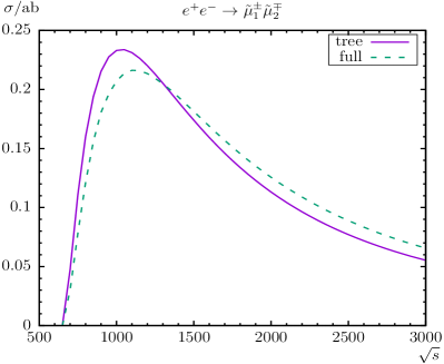
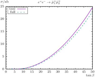
Figure 13: $\sigma(e^{+}e^{-}\to\tilde{\mu}^{\pm}_{1}\tilde{\mu}^{\mp}_{2})$. Tree-level and full one-loop corrected cross sections are shown with parameters chosen according to $\mathcal{S}$; see Tab. 1. The plots show the cross sections with $\sqrt{s}$ (left) and $M_{\tilde{E}}$ (right) varied. All masses and energies are in GeV and the cross sections are in atobarn.

The process $e^{+}e^{-}\to\tilde{\mu}^{\pm}_{1}\tilde{\mu}^{\mp}_{2}$ is shown in Fig. 13. It should be noted that the smuon (and stau) tree-level process consist of only one $Z$ exchange diagram (see Fig. 1) and is

$$\sigma_{\text{tree}} \propto|U^{\mathrm{\tilde{e}}_{g}}_{22}U^{\mathrm{\tilde{e}}_{g}*}_{12}|^{2}=|-U^{\mathrm{\tilde{e}}_{g}}_{21}U^{\mathrm{\tilde{e}}_{g}*}_{11}|^{2}=\frac{m_{\mathrm{e}_{g}}^{2}|A_{\mathrm{e}_{g}}-\mu^{*}t_{\beta}|^{2}}{(m_{\mathrm{\tilde{e}}_{g1}}^{2}-m_{\mathrm{\tilde{e}}_{g2}}^{2})^{2}}\,,$$ (25)

with the generation index $g=2,3$. (In the case of selectrons there is an additional tree-level diagram with neutralino exchange; see Fig. 1.) Setting $M_{\tilde{L}}=M_{\tilde{E}}+m$ and neglecting off-diagonal contributions, $D$-terms, and $m_{\mathrm{e}_{g}}^{2}$ contributions in the slepton mass matrix, yields

$$(m_{\mathrm{\tilde{e}}_{g1}}^{2}-m_{\mathrm{\tilde{e}}_{g2}}^{2})^{2} =m^{2}\,(2M_{\tilde{E}}+m+\ldots)^{2}+\ldots\,,$$ (26)

and consequently

$$\sigma_{\text{tree}} \propto\frac{m_{\mathrm{e}_{g}}^{2}|A_{\mathrm{e}_{g}}-\mu^{*}t_{\beta}|^{2}}{m^{2}\,(2M_{\tilde{E}}+m+\ldots)^{2}+\ldots}\propto\frac{m_{\mathrm{e}_{g}}^{2}}{m^{2}}\,.$$ (27)

For vanishing $m$ the cross section can be relatively large (but remains finite).

In our scenario $\mathcal{S}$ we have chosen a (more realistic) setting with $M_{\tilde{L}}\neq M_{\tilde{E}}$ (with an off-set of $m=50\,\,\mathrm{GeV}$). Therefore within this scenario the cross section for $e^{+}e^{-}\to\tilde{\mu}^{\pm}_{1}\tilde{\mu}^{\mp}_{2}$ turns out to be strongly suppressed by $m_{\mu}^{2}/m^{2}$, of ${\cal O}(0.1\,\mbox{ab})$; see the left plot in Fig. 13. This is below the reach of a linear collider. For this reason we refrain from a more detailed discussion here. The only expected exception is the variation with $t_{\beta}$ (see footnote 10) which we show in the right plot of Fig. 13. The loop corrected cross section increases from ${\cal O}(0.01\,\mbox{ab})$ at small $t_{\beta}$ to $\sim 23\,\mbox{ab}$ at $t_{\beta}=50$, as expected. The relative corrections for the $t_{\beta}$ dependence are increasing from $\sim-12\,\%$ at $t_{\beta}=10$ to $\sim-7\,\%$ at $t_{\beta}=50$.

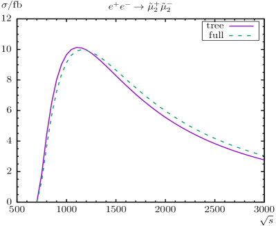
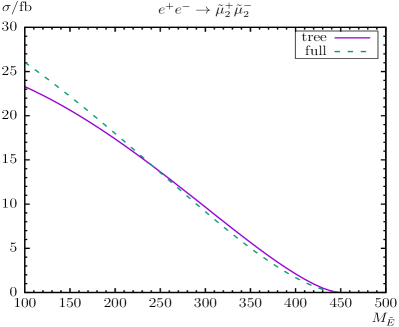
Figure 14: $\sigma(e^{+}e^{-}\to\tilde{\mu}^{+}_{2}\tilde{\mu}^{-}_{2})$. Tree-level and full one-loop corrected cross sections are shown with parameters chosen according to $\mathcal{S}$; see Tab. 1. The plots show the cross sections with $\sqrt{s}$ (left) and $M_{\tilde{E}}$ (right) varied. All masses and energies are in GeV.

Now we turn to the process $e^{+}e^{-}\to\tilde{\mu}^{+}_{2}\tilde{\mu}^{-}_{2}$ shown in Fig. 14. As a function of $\sqrt{s}$ (left plot) we find relative corrections of $\sim-5\,\%$ at $\sqrt{s}=1000\,\,\mathrm{GeV}$ (i.e. $\mathcal{S}$), and $\sim+10\,\%$ at $\sqrt{s}=3000\,\,\mathrm{GeV}$ with a tree crossing at $\sqrt{s}\approx 1200\,\,\mathrm{GeV}$.

In the analysis as a function of $M_{\tilde{E}}$ (right plot) the cross section is decreasing with increasing $M_{\tilde{E}}$, but can vary roughly by a factor of two w.r.t. $\mathcal{S}$. The full (relative) one-loop correction has its maximum of $\sim 26\,\mbox{fb}$ ($\sim+12\,\%$) at $M_{\tilde{E}}=100\,\,\mathrm{GeV}$, decreasing to $\sim 0.1\,\mbox{fb}$ ($\sim-40\,\%$) at $M_{\tilde{L}}=440\,\,\mathrm{GeV}$ with a tree crossing at $M_{\tilde{E}}\approx 245\,\,\mathrm{GeV}$.

The dependence on the other parameters is again (rather) negligible and therefore not shown here.

Turning to the third generation charged slepton production, the process $e^{+}e^{-}\to\tilde{\tau}^{+}_{1}\tilde{\tau}^{-}_{1}$ is shown in Fig. 15. As a function of $\sqrt{s}$ we find loop corrections of $\sim+14\,\%$ at $\sqrt{s}=1000\,\,\mathrm{GeV}$ (i.e. $\mathcal{S}$), a tree crossing at $\sqrt{s}\approx 725\,\,\mathrm{GeV}$ (where the one-loop corrections are between $\pm 10\,\%$ for $\sqrt{s}\;\raisebox{-3.00003pt}{$\stackrel{{\scriptstyle\displaystyle<}}{{\sim}}$}\;900\,\,\mathrm{GeV}$) and $\sim+35\,\%$ at $\sqrt{s}=3000\,\,\mathrm{GeV}$, very similar to $e^{+}e^{-}\to\tilde{\mu}^{+}_{1}\tilde{\mu}^{-}_{1}$.

In the analysis as a function of $M_{\tilde{E}}$ (upper right plot) the cross sections are decreasing with increasing $M_{\tilde{E}}$ as obvious from kinematics and the full corrections have their maximum of $\sim 28\,\mbox{fb}$ at $M_{\tilde{E}}=100\,\,\mathrm{GeV}$, more than two times larger than in $\mathcal{S}$. The relative corrections are changing from $\sim+33\,\%$ at $M_{\tilde{E}}=100\,\,\mathrm{GeV}$ to $\sim-25\,\%$ at $M_{\tilde{E}}=490\,\,\mathrm{GeV}$ with a tree crossing at $M_{\tilde{E}}=415\,\,\mathrm{GeV}$.

Here we show in the lower left plot of Fig. 15 the dependence on $t_{\beta}$. Contrary to other slepton production cross sections analyzed before, $\sigma_{\text{full}}(e^{+}e^{-}\to\tilde{\tau}^{+}_{1}\tilde{\tau}^{-}_{1})$ increases with $t_{\beta}$. The relative corrections for the $t_{\beta}$ dependence vary between $\sim+14.2\,\%$ at $t_{\beta}=5$ and $\sim+13.4\,\%$ at $t_{\beta}=50$.

The phase dependence $\varphi_{A_{\mathrm{e}_{g}}}$ of the cross section in $\mathcal{S}$ is shown in the lower right plot of Fig. 15. The loop correction increases the tree-level result by $\sim+14\,\%$. The phase dependence of the relative loop correction is very small and found to be below $0.2\,\%$. The variation with $\varphi_{M_{1}}$ is negligible and therefore not shown here.

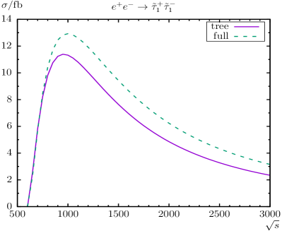
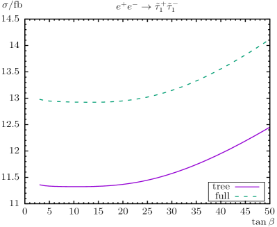
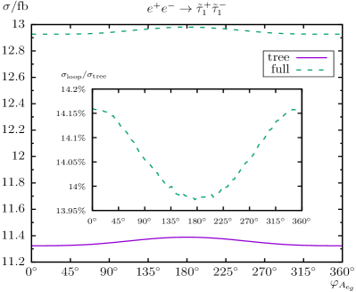
Figure 15: $\sigma(e^{+}e^{-}\to\tilde{\tau}^{+}_{1}\tilde{\tau}^{-}_{1})$. Tree-level and full one-loop corrected cross sections are shown with parameters chosen according to $\mathcal{S}$; see Tab. 1. The upper plots show the cross sections with $\sqrt{s}$ (left) and $M_{\tilde{E}}$ (right) varied; the lower plots show $t_{\beta}$ (left) and $\varphi_{A_{\mathrm{e}_{g}}}$ (right) varied. All masses and energies are in GeV.

The process $e^{+}e^{-}\to\tilde{\tau}^{\pm}_{1}\tilde{\tau}^{\mp}_{2}$ is shown in Fig. 16. The overall size of this cross section turns out to be rather small, including all analyzed parameter variations, but enhanced w.r.t. $e^{+}e^{-}\to\tilde{\mu}^{\pm}_{1}\tilde{\mu}^{\mp}_{2}$ by about a factor of $m_{\tau}^{2}/m_{\mu}^{2}$; see Eq. (27). The loop corrections have a noticeable impact, as can be seen in all six panels of Fig. 16, but never lift the cross section above $2\,\mbox{fb}$.

As a function of $\sqrt{s}$ (upper left plot) we find relative corrections of $\sim-11\,\%$ at $\sqrt{s}=1000\,\,\mathrm{GeV}$ (i.e. $\mathcal{S}$), and $\sim+19\,\%$ at $\sqrt{s}=3000\,\,\mathrm{GeV}$ with a tree crossing at $\sqrt{s}\approx 1300\,\,\mathrm{GeV}$.

As for other slepton production cross sections, $\sigma(e^{+}e^{-}\to\tilde{\tau}^{\pm}_{1}\tilde{\tau}^{\mp}_{2})$ depends strongly on $M_{\tilde{E}}$, where values one order of magnitude larger than in $\mathcal{S}$ (with $M_{\tilde{E}}=300\,\,\mathrm{GeV}$) are possible for small $M_{\tilde{E}}$. One can see that the full corrections have their maximum of $\sim 0.8\,\mbox{fb}$ at $M_{\tilde{E}}=100\,\,\mathrm{GeV}$. The relative corrections are decreasing from $\sim+6\,\%$ at $M_{\tilde{E}}=100\,\,\mathrm{GeV}$ to $\sim-51\,\%$ at $M_{\tilde{E}}=470\,\,\mathrm{GeV}$ with a tree crossing at $M_{\tilde{E}}\approx 170\,\,\mathrm{GeV}$.

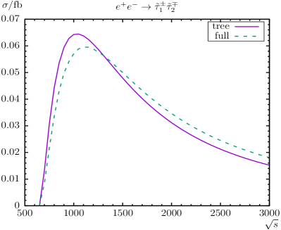
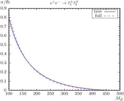
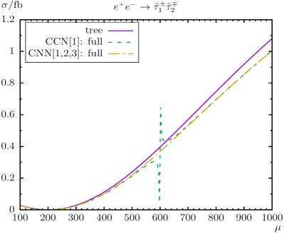
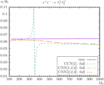
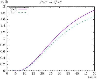
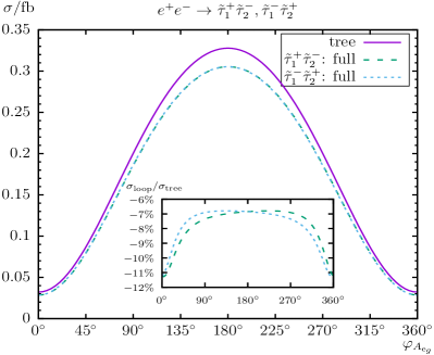
Figure 16: $\sigma(e^{+}e^{-}\to\tilde{\tau}^{\pm}_{1}\tilde{\tau}^{\mp}_{2})$. Tree-level and full one-loop corrected cross sections are shown with parameters chosen according to $\mathcal{S}$; see Tab. 1. The upper plots show the cross sections with $\sqrt{s}$ (left) and $M_{\tilde{E}}$ (right) varied; the middle plots show $\mu$ (left) and $M_{2}$ (right) varied; the lower plots show $t_{\beta}$ (left) and $\varphi_{A_{\mathrm{e}_{g}}}$ (right) varied. All masses and energies are in GeV.

With increasing $\mu$ in $\mathcal{S}$ (middle left plot) we find a nearly linear increase of the production cross section. While the CCN[1] scheme has its expected singularity at $\mu=600\,\,\mathrm{GeV}$, the CNN[1,2,3] scheme is smooth around this point. The relative loop corrections are nearly identical for both schemes and reach $\sim-10\,\%$ at $\mu=350\,\,\mathrm{GeV}$ (i.e. $\mathcal{S}$) and go up to $\sim-7\,\%$ at $\mu=1000\,\,\mathrm{GeV}$. It should be noted that the tree cross section is zero at $\mu=200\,\,\mathrm{GeV}$ where $U^{\mathrm{\tilde{e}}_{3}}_{11,22}=0$ ($U^{\mathrm{\tilde{e}}_{3}}_{12,21}=1$); see Eq. (25).

The $M_{2}$ dependence of the cross section in $\mathcal{S}$ is shown in the middle right plot. One can see again the (expected) breakdown of the CCN[1] scheme for $M_{2}=\mu=350\,\,\mathrm{GeV}$ and the smooth behavior of CNN[1,2,3] and CNN[2,2,3] around $M_{2}\sim\mu=350\,\,\mathrm{GeV}$. The loop corrections at the level of $\sim-5\,\%$ at $M_{2}=120\,\,\mathrm{GeV}$ and $\sim-7\,\%$ at $M_{2}=1000\,\,\mathrm{GeV}$ are found to be rather independent of $M_{2}$ within all three schemes. The tiny dip (hardly visible) at $M_{2}\approx 644\,\,\mathrm{GeV}$ in all three schemes is the chargino production threshold $m_{\tilde{\chi}_{1}^{\pm}}+m_{\tilde{\chi}_{2}^{\pm}}=\sqrt{s}=1000\,\,\mathrm{GeV}$.

Here we also show the variation with $t_{\beta}$ in the lower left plot of Fig. 16. The loop corrected cross section increases from ${\cal O}(0.1\,\mbox{ab})$ at small $t_{\beta}$ to $\sim 1.7\,\mbox{fb}$ at $t_{\beta}=50$. The relative corrections for the $t_{\beta}$ dependence are changing from $\sim-12\,\%$ at $t_{\beta}=10$ to $\sim-10\,\%$ at $t_{\beta}=50$.

The phase dependence $\varphi_{A_{\mathrm{e}_{g}}}$ of the cross section in $\mathcal{S}$ is shown in the lower right plot of Fig. 16. It is very pronounced and can vary $\sigma_{\text{full}}(e^{+}e^{-}\to\tilde{\tau}^{\pm}_{1}\tilde{\tau}^{\mp}_{2})$ from $0.03\,\mbox{fb}$ to $0.3\,\mbox{fb}$. The (relative) loop corrections are at the level of $\sim 10\,\%$ and vary with $\varphi_{A_{\mathrm{e}_{g}}}$ below $\pm 4.5\,\%$ w.r.t. the tree cross section. For our parameter set $\mathcal{S}$, with the complex phase $\varphi_{A_{\mathrm{e}_{g}}}$, the ${\cal CP}$ asymmetry turn out to be very small, as can be seen in the inlay.

Finally we turn to the process $e^{+}e^{-}\to\tilde{\tau}^{+}_{2}\tilde{\tau}^{-}_{2}$ shown in Fig. 17, which turns out to be sizable at the level of $10\,\mbox{fb}$. As a function of $\sqrt{s}$ (upper left plot) we find loop corrections of $\sim-5\,\%$ at $\sqrt{s}=1000\,\,\mathrm{GeV}$ (i.e. $\mathcal{S}$), and $\sim+10\,\%$ at $\sqrt{s}=3000\,\,\mathrm{GeV}$, with a tree crossing at $\sqrt{s}\approx 1200\,\,\mathrm{GeV}$.

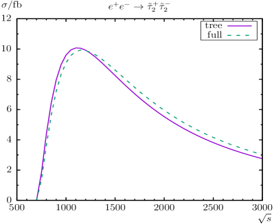
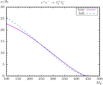
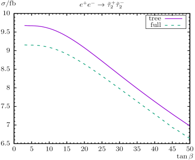
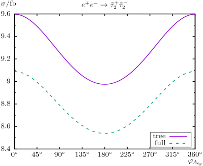
Figure 17: $\sigma(e^{+}e^{-}\to\tilde{\tau}^{+}_{2}\tilde{\tau}^{-}_{2})$. Tree-level and full one-loop corrected cross sections are shown with parameters chosen according to $\mathcal{S}$; see Tab. 1. The upper plots show the cross sections with $\sqrt{s}$ (left) and $M_{\tilde{E}}$ (right) varied; the lower plots show $t_{\beta}$ (left) and $\varphi_{A_{\mathrm{e}_{g}}}$ (right) varied. All masses and energies are in GeV.

The dependence on $M_{\tilde{E}}$ is shown in the upper right plot. The relative corrections are $\sim+12\,\%$ at $M_{\tilde{E}}=100\,\,\mathrm{GeV}$, $\sim-5\,\%$ at $M_{\tilde{E}}=300\,\,\mathrm{GeV}$ (i.e. $\mathcal{S}$), and $\sim-39\,\%$ at $M_{\tilde{E}}=440\,\,\mathrm{GeV}$, where the cross section goes to zero at $\mu=450\,\,\mathrm{GeV}$ (because of the choice $M_{\tilde{L}}=M_{\tilde{E}}+50\,\,\mathrm{GeV}$). The tree crossing is found at $\mu\approx 245\,\,\mathrm{GeV}$.

Again, here we show in the lower left plot of Fig. 17 the dependence on $t_{\beta}$. Contrary to other slepton production cross sections analyzed before, $\sigma_{\text{full}}(e^{+}e^{-}\to\tilde{\tau}^{+}_{2}\tilde{\tau}^{-}_{2})$ decreases with $t_{\beta}$. The relative corrections for the $t_{\beta}$ dependence vary between $\sim-5.4\,\%$ at $t_{\beta}=5$ and $\sim-4.4\,\%$ at $t_{\beta}=34$. A dip (not visible) in the dotted line at $t_{\beta}\approx 46$ is the threshold $m_{\tilde{\tau}_{1}}+M_{h}=m_{\tilde{\tau}_{2}}$.

The phase dependence $\varphi_{A_{\mathrm{e}_{g}}}$ of the cross section in $\mathcal{S}$ is shown in the lower right plot of Fig. 17. The loop correction decreases the tree-level result by $\sim-5\,\%$. The phase dependence of the relative loop correction is small and found to be below $0.5\,\%$. The variation with $\varphi_{M_{1}}$ is (again) negligible and therefore not shown here.

Overall, for the charged slepton pair production we observed a decreasing cross section $\propto\ln{(s)}/s$ for the first and $\propto 1/s$ for the second and third slepton generations for $s\to\infty$; see Ref. [40]. The (loop corrected) cross sections for the slepton pair production can reach a level of ${\cal O}(10\,\mbox{fb})$, depending on the SUSY parameters, but is very small for the production of two different smuons $\mathrm{\tilde{\mu}}_{1}\mathrm{\tilde{\mu}}_{2}$ at the ${\cal O}(10\,\mbox{ab})$. This renders these processes difficult to observe at an $e^{+}e^{-}$ collider. The full one-loop corrections are very roughly $15\,\%$ of the tree-level results, but vary strongly on the size of $M_{\tilde{E}}$ and in the case of selectrons also on the size of $M_{1}$ and $M_{2}$. Depending on the size of in particular these parameters the loop corrections can be either positive or negative. This shows that the loop corrections, while being large, have to be included point-by-point in any precision analysis. The dependence on $\varphi_{M_{1}}$ ($\varphi_{A_{\mathrm{e}_{g}}}$) was found at the level of $\sim 15\,\%$ ($\sim 8\,\%$), but can go up to $\sim 18\,\%$ ($\sim 14\,\%$) for the extreme cases. The relative loop corrections varied by up to $2\,\%$ ($4\,\%$) with $\varphi_{M_{1}}$ ($\varphi_{A_{\mathrm{e}_{g}}}$). Consequently, the complex phase dependence must be taken into account as well. Finally, for our parameter set $\mathcal{S}$ the ${\cal CP}$ asymmetries turn out to be very small, well below $\pm 1\,\%$ (hardly measurable in future $e^{+}e^{-}$ collider experiments).

For all parameter choices it was possible to identify at least one renormalization scheme that exhibited a “smooth” behavior. It appears to be possible for any parameter variation to find a combination of schemes that yield a numerically stable (and nearly constant) one-loop level contribution. A detailed analysis of which scheme yields this desired behavior as a function of the underlying SUSY parameters, however, is beyond the scope of this paper.

4.3 The process $e^{+}e^{-}\to\tilde{\nu}_{g}\tilde{\nu}_{g}^{*}$

In Figs. 18 – (20) we present the results for scalar neutrino production at $e^{+}e^{-}$ colliders. It should be noted that for $s\to\infty$ decreasing cross sections $\propto\ln{(s)}/s$ for the first and $\propto 1/s$ for the second and third slepton generations are expected; see Ref. [41]. We start with the process $e^{+}e^{-}\to\tilde{\nu}_{e}\tilde{\nu}_{e}^{*}$ that is shown in Fig. 18.

In the analysis of the production cross section as a function of $\sqrt{s}$ (upper left plot) we find the expected behavior: a strong rise close to the production threshold, followed by a decrease with increasing $\sqrt{s}$, where the $s$-channel dominates. We find a very small shift w.r.t. $\sqrt{s}$ around the production threshold. Away from the production threshold, loop corrections of $\sim-12\,\%$ at $\sqrt{s}=1000\,\,\mathrm{GeV}$ are found in scenario $\mathcal{S}$ (see Tab. 1). The relative size of the loop corrections increase up to $\sim-8\,\%$ at $\sqrt{s}=1650\,\,\mathrm{GeV}$ and then reach $\sim-10\,\%$ at $\sqrt{s}=3000\,\,\mathrm{GeV}$.

The cross section as a function of $M_{\tilde{E}}$ is shown in the upper right plot of Fig. 18. The masses of the electron sneutrinos are governed by $M_{\tilde{L}}=M_{\tilde{E}}+50\,\,\mathrm{GeV}$. Consequently, a strong, nearly linear decrease can be observed from $\sim 140\,\mbox{fb}$ down to zero for $M_{\tilde{E}}=450\,\,\mathrm{GeV}$ (i.e. the sneutrino production threshold), as can be expected from kinematics. In scenario $\mathcal{S}$ we find a non-negligible decrease of the cross sections from the loop corrections. They start at $M_{\tilde{E}}=100\,\,\mathrm{GeV}$ with $\sim-3\,\%$ and reach $\sim-53\,\%$ at $M_{\tilde{E}}\approx 450\,\,\mathrm{GeV}$. In the latter case these large loop corrections are due to the (relative) smallness of the tree-level results, which goes to zero at the sneutrino production threshold.

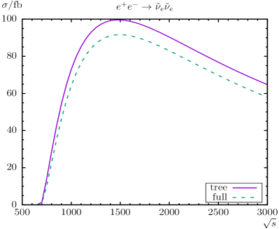
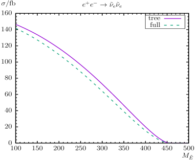
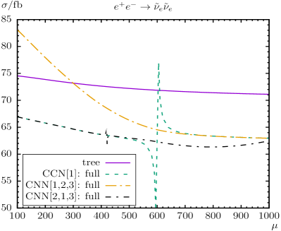
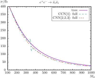
Figure 18: $\sigma(e^{+}e^{-}\to\tilde{\nu}_{e}\tilde{\nu}_{e}^{*})$. Tree-level and full one-loop corrected cross sections are shown with parameters chosen according to $\mathcal{S}$; see Tab. 1. The upper plots show the cross sections with $\sqrt{s}$ (left) and $M_{\tilde{E}}$ (right) varied; the lower plots show $\mu$ (left) and $M_{2}$ (right) varied. All masses and energies are in GeV.

With increasing $\mu$ in $\mathcal{S}$ (lower left plot) we find a small, rather linear decrease of the production cross section within CCN[1], mainly induced by the change in the chargino $t$-channel contribution ($\tilde{\chi}_{2}^{\pm}$ is dominant for $\mu\;\raisebox{-3.00003pt}{$\stackrel{{\scriptstyle\displaystyle<}}{{\sim}}$}\;570\,\,\mathrm{GeV}$ and $\tilde{\chi}_{1}^{\pm}$ dominant for $\mu\;\raisebox{-3.00003pt}{$\stackrel{{\scriptstyle\displaystyle>}}{{\sim}}$}\;570\,\,\mathrm{GeV}$). The relative loop corrections within CCN[1] (green dashed line) reach $\sim-10\,\%$ at $\mu=100\,\,\mathrm{GeV}$ (at the border of the experimental limit), $\sim-12\,\%$ at $\mu=350\,\,\mathrm{GeV}$ (i.e. $\mathcal{S}$) and $\sim-11.5\,\%$ at $\mu=1000\,\,\mathrm{GeV}$. While CCN[1] is unreliable for $500\,\,\mathrm{GeV}<\mu<700\,\,\mathrm{GeV}$, CNN[2,1,3] (black dash-dotted line) yields reliable higher-order corrections for $\mu<600\,\,\mathrm{GeV}$ and CNN[1,2,3] (yellow dash-dotted line) for $\mu>600\,\,\mathrm{GeV}$; as can be seen in the lower left plot of Fig. 18. Again, in the CNN[2,1,3] scheme $\delta\mu$ has a strong minimum at $\mu\approx 421\,\,\mathrm{GeV}$, dominating the loop corrections.

The dependence $M_{2}$ of the cross section in $\mathcal{S}$ is shown in the lower right plot of Fig. 18, where again the chargino $t$-channel exchange plays a dominant role ($\tilde{\chi}_{1}^{\pm}$ is dominant for $M_{2}\;\raisebox{-3.00003pt}{$\stackrel{{\scriptstyle\displaystyle<}}{{\sim}}$}\;380\,\,\mathrm{GeV}$ and $\tilde{\chi}_{2}^{\pm}$ dominant for $M_{2}\;\raisebox{-3.00003pt}{$\stackrel{{\scriptstyle\displaystyle>}}{{\sim}}$}\;380\,\,\mathrm{GeV}$). Again, one can see the (expected) breakdown of the CCN[1] scheme for $M_{2}=\mu=350\,\,\mathrm{GeV}$. Outside the region $M_{2}\approx\mu$ the scheme CCN[1] is expected to be reliable, since each of the three OS conditions is strongly connected to one of the three input parameters, $|M_{1}|$, $M_{2}$ and $\mu$. The loop corrections are $\sim-12\,\%$ at $M_{2}=600\,\,\mathrm{GeV}$ (i.e. $\mathcal{S}$) and $\sim-14\,\%$ at $M_{2}=1000\,\,\mathrm{GeV}$, with a tree crossing at $M_{2}\approx 130\,\,\mathrm{GeV}$. The CNN[2,2,3] scheme (red dashed line) is smooth for all values of $M_{2}$ shown and a perfect approximation for CCN[1].

Due to the absence of $\varphi_{M_{1}}$ in the tree-level production cross section the effect of this complex phase is expected to be small. Correspondingly we find that the phase dependence $\varphi_{M_{1}}$ of the cross section in our scenario is tiny. The same holds for the variation with $\varphi_{A_{\mathrm{e}_{g}}}$, it also remains tiny and unobservable. Therefore we omit showing these two complex phases explicitely.

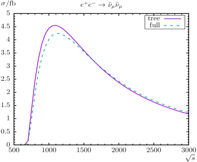
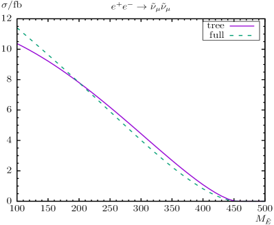
Figure 19: $\sigma(e^{+}e^{-}\to\tilde{\nu}_{\mu}\tilde{\nu}_{\mu}^{*})$. Tree-level and full one-loop corrected cross sections are shown with parameters chosen according to $\mathcal{S}$; see Tab. 1. The plots show the cross sections with $\sqrt{s}$ (left) and $M_{\tilde{E}}$ (right) varied. All masses and energies are in GeV.

In Fig. 19 we present the cross sections $\sigma(e^{+}e^{-}\to\tilde{\nu}_{\mu}\tilde{\nu}_{\mu}^{*})$. In the analysis as a function of $\sqrt{s}$ (left plot) we find as before a tiny shift w.r.t. $\sqrt{s}$, where the position of the maximum cross section shifts by about $+50\,\,\mathrm{GeV}$. The relative corrections are found to be of $\sim-9\,\%$ at $\sqrt{s}=1000\,\,\mathrm{GeV}$ (i.e. $\mathcal{S}$), and $\sim+5\,\%$ at $\sqrt{s}=3000\,\,\mathrm{GeV}$.

As a function of $M_{\tilde{E}}$ (right plot) the cross section decreases rather linearly. The relative corrections change from $\sim+10\,\%$ at $M_{\tilde{E}}=100\,\,\mathrm{GeV}$ to $\sim-60\,\%$ at $M_{\tilde{E}}=450\,\,\mathrm{GeV}$, with a tree crossing at $M_{\tilde{E}}\approx 200\,\,\mathrm{GeV}$.

The dependence on the other parameters is (again) negligible and therefore not shown here.

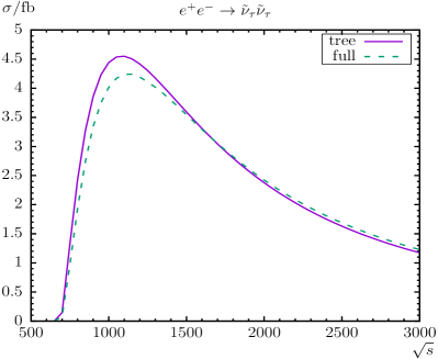
Figure 20: $\sigma(e^{+}e^{-}\to\tilde{\nu}_{\tau}\tilde{\nu}_{\tau}^{*})$. Tree-level and full one-loop corrected cross sections are shown with parameters chosen according to $\mathcal{S}$; see Tab. 1. The plots show the cross sections with $\sqrt{s}$ (left) and $M_{\tilde{E}}$ (right) varied. All masses and energies are in GeV.

We finish the $e^{+}e^{-}\to\tilde{\nu}_{g}\tilde{\nu}_{g}^{*}$ analysis with $\sigma(e^{+}e^{-}\to\tilde{\nu}_{\tau}\tilde{\nu}_{\tau}^{*})$ in Fig. 20. The results are very similar as for $\sigma(e^{+}e^{-}\to\tilde{\nu}_{\mu}\tilde{\nu}_{\mu}^{*})$ (see above), since the sneutrino masses are the same for all three generations, as are the contributing higher-order diagrams.

Overall, for the sneutrino pair production we observed a decreasing cross section $\propto\ln{(s)}/s$ for the first and $\propto 1/s$ for the second and third slepton generations for $s\to\infty$; see Ref. [41]. The full one-loop corrections are very roughly $10\,\%$ of the tree-level results, but depend strongly on the size of $M_{\tilde{E}}$, where larger values result even in negative loop corrections. The cross sections are largest for $e^{+}e^{-}\to\tilde{\nu}_{e}\tilde{\nu}_{e}^{*}$ and roughly smaller by one order of magnitude for $e^{+}e^{-}\to\tilde{\nu}_{\mu}\tilde{\nu}_{\mu}^{*}$ and $e^{+}e^{-}\to\tilde{\nu}_{\tau}\tilde{\nu}_{\tau}^{*}$. This is caused by the absence of the chargino $t$-channel diagram (i.e. a $\tilde{\chi}_{c}^{\mp}\,e^{\pm}\,\tilde{\nu}_{g}$ coupling), which only contributes to $e^{+}e^{-}\to\tilde{\nu}_{e}\tilde{\nu}_{e}^{*}$; see Fig. 1. The variation of the cross sections with $\varphi_{M_{1}}$ and $\varphi_{A_{\mathrm{e}_{g}}}$ is found extremely small and have not been shown explicitely.

As for charged slepton production, for all parameter choices it was possible to identify at least one renormalization scheme that exhibited a “smooth” behavior. Also for sneutrino production it appears to be possible for any parameter variation to find a combination of schemes that yield numerically stable (and nearly constant) one-loop level contributions.

5 Conclusions

We have evaluated all slepton production modes at $e^{+}e^{-}$ colliders with a two-particle final state, i.e. $e^{+}e^{-}\to\mathrm{\tilde{e}}^{\pm}_{gs}\mathrm{\tilde{e}}^{\mp}_{gs^{\prime}}$ and $e^{+}e^{-}\to\tilde{\nu}_{g}\tilde{\nu}_{g}^{*}$ allowing for complex parameters. In the case of discovery of sleptons a subsequent precision measurement of their properties will be crucial to determine their nature and the underlying (SUSY) parameters. In order to yield sufficient accuracy, one-loop corrections to the various slepton production modes have to be considered. This is particularly the case for the anticipated high accuracy of the slepton property determination at $e^{+}e^{-}$ colliders [22].

The evaluation of the processes (1) and (2) is based on a full one-loop calculation, also including hard, soft and collinear QED radiation. The renormalization is chosen to be identical as for the slepton decay calculations [28], or slepton production from heavy Higgs-boson decay [29], as well as from chargino and neutralino decays [30, 31, 32, 33]. Consequently, the predictions for the production and decay can be used together in a consistent manner (e.g., in a global phenomenological analysis of the slepton sector at the one-loop level).

We first briefly reviewed the relevant sectors including some details of the one-loop renormalization procedure of the cMSSM, which are relevant for our calculation. In most cases we follow Ref. [49]. We have discussed the calculation of the one-loop diagrams, the treatment of UV, IR, and collinear divergences that are canceled by the inclusion of (hard, soft, and collinear) QED radiation. As far as possible we have checked our result against the literature, and in most cases where a meaningful comparison could be performed we found good agreement; parts of the differences can be attributed to problems with input parameters and/or different renormalization schemes (conversions).

For the analysis we have chosen a standard parameter set (see Tab. 1), which allows for the production of all combinations of sleptons at an $e^{+}e^{-}$ collider with a center-of-mass energy up to $\sqrt{s}=1000\,\,\mathrm{GeV}$. In the analysis we investigated the variation of the various production cross sections with the center-of-mass energy $\sqrt{s}$, the Higgs mixing parameter $\mu$, the gaugino mass parameters $|M_{1}|$ and/or $M_{2}$, the slepton soft SUSY-breaking parameter $M_{\tilde{E}}$ ($M_{\tilde{L}}=M_{\tilde{E}}+50\,\,\mathrm{GeV}$) and the complex phases $\varphi_{A_{\mathrm{e}_{g}}}$ (of the trilinear Higgs-slepton coupling, $A_{\mathrm{e}_{g}}$; $g=1,2,3$) and $\varphi_{M_{1}}$ (of the gaugino mass parameter $M_{1}$), respectively. Where relevant we also showed the variation with $t_{\beta}$.

In our numerical scenarios we compared the tree-level production cross sections with the full one-loop corrected cross sections. The numerical results we have shown are, of course, dependent on the choice of the SUSY parameters. Nevertheless, they give an idea of the relevance of the full one-loop corrections. For the slepton pair production, $e^{+}e^{-}\to\mathrm{\tilde{e}}^{\pm}_{gs}\mathrm{\tilde{e}}^{\mp}_{gs^{\prime}}$ and $e^{+}e^{-}\to\tilde{\nu}_{g}\tilde{\nu}_{g}^{*}$ we observed for $s\to\infty$ a decreasing cross section $\propto\ln{(s)}/s$ for the first and $\propto 1/s$ for the second and third slepton generations. The (loop corrected) cross sections for the charged slepton pair production can reach a level of $10\,\mbox{fb}$, depending on the SUSY parameters, but is very small for the production of two different smuons $\mathrm{\tilde{\mu}}_{1}\mathrm{\tilde{\mu}}_{2}$ at the ${\cal O}(10\,\mbox{ab})$ (and with the cross section of ${\tilde{\tau}_{1}}{\tilde{\tau}_{2}}$ enhanced by a factor of $m_{\tau}^{2}/m_{\mu}^{2}$). This renders these processes difficult to observe at an $e^{+}e^{-}$ collider. The full one-loop corrections are very roughly $15\,\%$ of the tree-level results, but vary strongly on the size of $M_{\tilde{E}}$ and in the case of selectrons also on the size of $M_{1}$ and $M_{2}$. Depending on the size of in particular these parameters the loop corrections can be either positive or negative. The dependence on $\varphi_{M_{1}}$ ($\varphi_{A_{\mathrm{e}_{g}}}$) was found at the level of $\sim 15\,\%$ ($\sim 8\,\%$), but can go up to $\sim 18\,\%$ ($\sim 14\,\%$) for the extreme cases. The relative loop corrections varied by up to $2\,\%$ ($4\,\%$) with $\varphi_{M_{1}}$ ($\varphi_{A_{\mathrm{e}_{g}}}$). This shows that the loop corrections, including the complex phase dependence, have to be included point-by-point in any precision analysis, or any precise determination of SUSY parameters from the production of cMSSM sleptons at $e^{+}e^{-}$ linear colliders.

Concerning scalar neutrino production, the full one-loop corrections are very roughly $10\,\%$ of the tree-level results, but depend strongly on the size of $M_{\tilde{E}}$, where larger values result even in negative loop corrections. The cross sections are largest for $e^{+}e^{-}\to\tilde{\nu}_{e}\tilde{\nu}_{e}^{*}$ and roughly smaller by one order of magnitude for $e^{+}e^{-}\to\tilde{\nu}_{\mu}\tilde{\nu}_{\mu}^{*}$ and $e^{+}e^{-}\to\tilde{\nu}_{\tau}\tilde{\nu}_{\tau}^{*}$. The variation of the cross sections with $\varphi_{M_{1}}$ and $\varphi_{A_{\mathrm{e}_{g}}}$ is found extremely small. Also for scalar neutrino production the loop corrections have to be included point-by-point in any precision analysis at $e^{+}e^{-}$ linear colliders.

For all cross section calculations and for all parameter choices it was possible to identify at least one renormalization scheme that exhibited a “smooth” behavior. It appears to be possible for any parameter variation to find a combination of schemes that yield numerically stable (and nearly constant) one-loop level contributions. A detailed analysis of which scheme yields this desired behavior as a function of the underlying SUSY parameters, however, is beyond the scope of this paper.

We emphasize again that our full one-loop calculation can readily be used together with corresponding full one-loop corrections to slepton decays [28] or other slepton production modes [29, 30, 31, 32, 33].

Acknowledgements

We thank T. Hahn and F. von der Pahlen for helpful discussions. The work of S.H. is supported in part by the MEINCOP Spain under contract FPA2016-78022-P, in part by the “Spanish Agencia Estatal de Investigaci?n” (AEI) and the EU “Fondo Europeo de Desarrollo Regional” (FEDER) through the project FPA2016-78022-P, and in part by the AEI through the grant IFT Centro de Excelencia Severo Ochoa SEV-2016-0597.

References

- [1]
- [2] H. Nilles, Phys. Rept. 110 (1984) 1.
- [3] R. Barbieri, Riv. Nuovo Cim. 11 (1988) 1.
- [4] H. Haber, G. Kane, Phys. Rept. 117 (1985) 75.
- [5] J. Gunion, H. Haber, Nucl. Phys. B 272 (1986) 1.
- [6] G. Aad et al. [ATLAS Collaboration], Phys. Lett. B 716 (2012) 1 [arXiv:1207.7214 [hep-ex]].
- [7] S. Chatrchyan et al. [CMS Collaboration], Phys. Lett. B 716 (2012) 30 [arXiv:1207.7235 [hep-ex]].
- [8] H. Goldberg, Phys. Rev. Lett. 50 (1983) 1419.
- [9] J. Ellis, J. Hagelin, D. Nanopoulos, K. Olive, M. Srednicki, Nucl. Phys. B 238 (1984) 453.
- [10] A. Pilaftsis, Phys. Rev. D 58 (1998) 096010 [arXiv:hep-ph/9803297].
- [11] A. Pilaftsis, Phys. Lett. B 435 (1998) 88 [arXiv:hep-ph/9805373].
- [12] D. A. Demir, Phys. Rev. D 60 (1999) 055006 [arXiv:hep-ph/9901389].
- [13] A. Pilaftsis, C. E. M. Wagner, Nucl. Phys. B 553 (1999) 3 [arXiv:hep-ph/9902371].
- [14] S. Heinemeyer, Eur. Phys. J. C 22 (2001) 521 [arXiv:hep-ph/0108059].
- [15] https://twiki.cern.ch/twiki/bin/view/AtlasPublic/SupersymmetryPublicResults .
- [16] https://twiki.cern.ch/twiki/bin/view/CMSPublic/PhysicsResultsSUS .
- [17] H. Baer et al., The International Linear Collider Technical Design Report - Volume 2: Physics, arXiv:1306.6352 [hep-ph].
-
[18]
R.-D. Heuer et al. [TESLA Collaboration],
TESLA Technical Design Report, Part III: Physics at an Linear Collider,
arXiv:hep-ph/0106315, see:
http://tesla.desy.de/new_pages/TDR_CD/start.html . - [19] K. Ackermann et al., Proceedings Summer Colloquium, Amsterdam, Netherlands, 4 April 2003, DESY-PROC-2004-01.
- [20] J. Brau et al. [ILC Collaboration], ILC Reference Design Report Volume 1 - Executive Summary, arXiv:0712.1950 [physics.acc-ph].
- [21] A. Djouadi et al. [ILC Collaboration], International Linear Collider Reference Design Report Volume 2: Physics at the ILC, arXiv:0709.1893 [hep-ph].
- [22] G. Moortgat-Pick et al., Eur. Phys. J. C 75 (2015) 8, 371 [arXiv:1504.01726 [hep-ph]].
- [23] L. Linssen, A. Miyamoto, M. Stanitzki, H. Weerts, arXiv:1202.5940 [physics.ins-det].
- [24] H. Abramowicz et al. [CLIC Detector and Physics Study Collaboration], Physics at the CLIC Linear Collider – Input to the Snowmass process 2013, arXiv:1307.5288 [hep-ex].
- [25] G. Weiglein et al. [LHC/ILC Study Group], Phys. Rept. 426 (2006) 47 [arXiv:hep-ph/0410364].
- [26] A. De Roeck et al., Eur. Phys. J. C 66 (2010) 525 [arXiv:0909.3240 [hep-ph]].
- [27] A. De Roeck, J. Ellis, S. Heinemeyer, CERN Cour. 49N10 (2009) 27.
- [28] S. Heinemeyer, C. Schappacher, Eur. Phys. J. C 72 (2012) 2136 [arXiv:1204.4001 [hep-ph]].
- [29] S. Heinemeyer, C. Schappacher, Eur. Phys. J. C 75 (2015) 5, 198 [arXiv:1410.2787 [hep-ph]].
- [30] S. Heinemeyer, F. von der Pahlen, C. Schappacher, Eur. Phys. J. C 72 (2012) 1892 [arXiv:1112.0760 [hep-ph]].
- [31] S. Heinemeyer, F. von der Pahlen, C. Schappacher, arXiv:1202.0488 [hep-ph].
- [32] A. Bharucha, S. Heinemeyer, F. von der Pahlen, C. Schappacher, Phys. Rev. D 86 (2012) 075023 [arXiv:1208.4106 [hep-ph]].
- [33] A. Bharucha, S. Heinemeyer, F. von der Pahlen, Eur. Phys. J. C 73 (2013) 2629 [arXiv:1307.4237 [hep-ph]].
- [34] D. H. Schiller, D. Wähner, Nucl.Phys. B 255 (1985) 505.
- [35] B. de Carlos, M. A. Diaz, Phys. Lett. B 417 (1998) 72 [arXiv:hep-ph/9511421].
- [36] S. Y. Choi, M. Drees, B. Gaissmaier, J. S. Lee, Phys. Rev. D 64 (2001) 095009 [arXiv:hep-ph/0103284].
- [37] A. Freitas, D. J. Miller, P. M. Zerwas, Eur. Phys. J. C 21 (2001) 361 [arXiv:hep-ph/0106198].
- [38] A. Freitas, “Production of scalar leptons at linera colliders”, PhD thesis, Hamburg, Germany, 2002.
- [39] C. Blöchinger, H. Fraas, G. Moortgat-Pick, W. Porod, Eur. Phys. J. C 24 (2002) 297 [arXiv:hep-ph/0201282].
- [40] A. Freitas, A. von Manteuffel, P. M. Zerwas, Eur. Phys. J. C 34 (2004) 487 [arXiv:hep-ph/0310182].
- [41] A. Freitas, A. von Manteuffel, P. M. Zerwas, Eur. Phys. J. C 40 (2005) 435 [arXiv:hep-ph/0408341].
- [42] A. Arhrib, W. Hollik, JHEP 0404 (2004) 073 [arXiv:hep-ph/0311149].
- [43] K. Kovařík, C. Weber, H. Eberl, W. Majerotto, Phys. Lett. B 591 (2004) 242 [arXiv:hep-ph/0401092].
- [44] K. Kovařík, “Precise predictions for sfermion pair production at a linear collider”, PhD thesis, Bratislava, Slovakia, 2005.
- [45] K. Kovařík, C. Weber, H. Eberl, W. Majerotto, Phys. Rev. D 72 (2005) 053010 [arXiv:hep-ph/0506021].
- [46] J. Küblbeck, M. Böhm, A. Denner, Comput. Phys. Commun. 60 (1990) 165.
- [47] T. Hahn, Comput. Phys. Commun. 140 (2001) 418 [arXiv:hep-ph/0012260].
-
[48]
T. Hahn, C. Schappacher,
Comput. Phys. Commun. 143 (2002) 54
[arXiv:hep-ph/0105349].
Program, user’s guide and model files are available via: http://www.feynarts.de . - [49] T. Fritzsche, T. Hahn, S. Heinemeyer, F. von der Pahlen, H. Rzehak, C. Schappacher, Comput. Phys. Commun. 185 (2014) 1529 [arXiv:1309.1692 [hep-ph]].
-
[50]
T. Hahn, M. Pérez-Victoria,
Comput. Phys. Commun. 118 (1999) 153
[arXiv:hep-ph/9807565].
Program and user’s guide are available via: http://www.feynarts.de/formcalc/ . - [51] T. Hahn, S. Paßehr, C. Schappacher, PoS LL2016 (2016) 068, J. Phys. Conf. Ser. 762 (2016) 1, 012065 [arXiv:1604.04611 [hep-ph]].
- [52] S. Heinemeyer, C. Schappacher, Eur. Phys. J. C 75 (2015) 5, 230 [arXiv:1503.02996 [hep-ph]].
- [53] S. Heinemeyer, H. Rzehak, C. Schappacher, Phys. Rev. D 82 (2010) 075010 [arXiv:1007.0689 [hep-ph]].
- [54] S. Heinemeyer, H. Rzehak, C. Schappacher, PoSCHARGED 2010 (2010) 039 [arXiv:1012.4572 [hep-ph]].
- [55] T. Fritzsche, S. Heinemeyer, H. Rzehak, C. Schappacher, Phys. Rev. D 86 (2012) 035014 [arXiv:1111.7289 [hep-ph]].
- [56] S. Heinemeyer, C. Schappacher, Eur. Phys. J. C 72 (2012) 1905 [arXiv:1112.2830 [hep-ph]].
- [57] S. Heinemeyer, C. Schappacher, Eur. Phys. J. C 76 (2016) 4, 220 [arXiv:1511.06002 [hep-ph]].
- [58] S. Heinemeyer, C. Schappacher, Eur. Phys. J. C 76 (2016) 10, 535 [arXiv:1606.06981 [hep-ph]].
- [59] S. Heinemeyer, C. Schappacher, Eur. Phys. J. C 77 (2017) 9, 649 [arXiv:1704.07627 [hep-ph]].
- [60] M. Frank, T. Hahn, S. Heinemeyer, W. Hollik, H. Rzehak, G. Weiglein, JHEP 0702 (2007) 047 [arXiv:hep-ph/0611326].
- [61] A. Denner, S. Dittmaier, M. Roth, D. Wackeroth, Nucl. Phys. B 560 (1999) 33 [arXiv:hep-ph/9904472].
- [62] F. del Aguila, A. Culatti, R. Muñoz-Tapia, M. Pérez-Victoria, Nucl. Phys. B 537 (1999) 561 [arXiv:hep-ph/9806451].
- [63] W. Siegel, Phys. Lett. B 84 (1979) 193.
- [64] D. Capper, D. Jones, P. van Nieuwenhuizen, Nucl. Phys. B 167 (1980) 479.
- [65] D. Stöckinger, JHEP 0503 (2005) 076 [arXiv:hep-ph/0503129].
- [66] W. Hollik, D. Stöckinger, Phys. Lett. B 634 (2006) 63 [arXiv:hep-ph/0509298].
- [67] A. Denner, Fortsch. Phys. 41 (1993) 307 [arXiv:0709.1075 [hep-ph]].
- [68] K. Fabricius, I. Schmitt, G. Kramer, G. Schierholz, Zeit. Phys. C 11 (1981) 315.
- [69] G. Kramer, B. Lampe, Fortschr. Phys. 37 (1989) 161.
- [70] H. Baer, J. Ohnemus, J. Owens, Phys. Rev. D 40 (1989) 2844.
- [71] B. Harris, J. Owens, Phys. Rev. D 65 (2002) 094032 [arXiv:hep-ph/0102128].
- [72] T. Hahn, Comput. Phys. Commun. 168 (2005) 78 [arXiv:hep-ph/0404043].
-
[73]
T. Hahn,
arXiv:1408.6373 [physics.comp-ph].
The program is available via: http://www.feynarts.de/cuba/ . - [74] S. Heinemeyer, W. Hollik and G. Weiglein, Comput. Phys. Commun. 124 (2000) 76 [arXiv:hep-ph/9812320].
- [75] S. Heinemeyer, W. Hollik and G. Weiglein, Eur. Phys. J. C 9 (1999) 343 [arXiv:hep-ph/9812472].
- [76] G. Degrassi, S. Heinemeyer, W. Hollik, P. Slavich and G. Weiglein, Eur. Phys. J. C 28 (2003) 133 [arXiv:hep-ph/0212020].
- [77] T. Hahn, S. Heinemeyer, W. Hollik, H. Rzehak and G. Weiglein, Comput. Phys. Commun. 180 (2009) 1426.
- [78] T. Hahn, S. Heinemeyer, W. Hollik, H. Rzehak and G. Weiglein, Phys. Rev. Lett. 112 (2014) 14, 141801 [arXiv:1312.4937 [hep-ph]].
- [79] H. Bahl and W. Hollik, Eur. Phys. J. C 76 (2016) 499 [arXiv:1608.01880 [hep-ph]].
- [80] H. Bahl, S. Heinemeyer, W. Hollik and G. Weiglein, Eur. Phys. J. C 78 (2018) no.1, 57 [arXiv:1706.00346 [hep-ph]].
- [81] R. Mertig, M. Böhm and A. Denner, Comput. Phys. Commun. 64 (1991) 345.
- [82] B. C. Allanach et al., Eur. Phys. J. C 25 (2002) 113 [arXiv:hep-ph/0202233].
- [83] C. Patrignani et al. (Particle Data Group), Chin. Phys. C 40 (2016 and 2017 update) 100001.
-
[84]
ATLAS Collaboration, ATLAS-CONF-2017-039, see:
https://atlas.web.cern.ch/Atlas/GROUPS/PHYSICS/CONFNOTES/ATLAS-CONF-2017-039 . -
[85]
CMS Collaboration, CMS-PAS-SUS-17-004, see:
http://cms-results.web.cern.ch/cms-results/public-results/preliminary-results/SUS-17-004/index.html . -
[86]
CMS Collaboration, CMS-PAS-SUS-16-039, see:
http://cms-results.web.cern.ch/cms-results/public-results/preliminary-results/SUS-16-039/index.html . - [87] J. Frère, D. Jones, S. Raby, Nucl. Phys. B 222 (1983) 11.
- [88] M. Claudson, L. Hall, I. Hinchliffe, Nucl. Phys. B 228 (1983) 501.
- [89] C. Kounnas, A. Lahanas, D. Nanopoulos, M. Quiros, Nucl. Phys. B 236 (1984) 438.
- [90] J. Gunion, H. Haber, M. Sher, Nucl. Phys. B 306 (1988) 1.
- [91] J. Casas, A. Lleyda, C. Muñoz, Nucl. Phys. B 471 (1996) 3 [arXiv:hep-ph/9507294].
- [92] P. Langacker, N. Polonsky, Phys. Rev. D 50 (1994) 2199 [arXiv:hep-ph/9403306].
- [93] A. Strumia, Nucl. Phys. B 482 (1996) 24 [arXiv:hep-ph/9604417].
- [94] M. Frank et al., Phys. Rev. D 88 (2013) 5, 055013 [arXiv:1306.1156 [hep-ph]].
- [95] S. Dimopoulos, S. Thomas, Nucl. Phys. B 465 (1996) 23 [arXiv:hep-ph/9510220].
- [96] M. Dugan, B. Grinstein, L. Hall, Nucl. Phys. B 255 (1985) 413.
- [97] D. Demir, O. Lebedev, K. Olive, M. Pospelov, A. Ritz, Nucl. Phys. B 680 (2004) 339 [arXiv:hep-ph/0311314].
- [98] D. Chang, W. Keung, A. Pilaftsis, Phys. Rev. Lett. 82 (1999) 900 [Erratum-ibid. 83 (1999) 3972] [arXiv:hep-ph/9811202].
- [99] A. Pilaftsis, Phys. Lett. B 471 (1999) 174 [arXiv:hep-ph/9909485].
- [100] O. Lebedev, K. Olive, M. Pospelov, A. Ritz, Phys. Rev. D 70 (2004) 016003 [arXiv:hep-ph/0402023].
- [101] W. Hollik, J. Illana, S. Rigolin, D. Stöckinger, Phys. Lett. B 416 (1998) 345 [arXiv:hep-ph/9707437].
- [102] W. Hollik, J. Illana, S. Rigolin, D. Stöckinger, Phys. Lett. B 425 (1998) 322 [arXiv:hep-ph/9711322].
- [103] P. Nath, Phys. Rev. Lett. 66 (1991) 2565.
- [104] Y. Kizukuri, N. Oshimo, Phys. Rev. D 46 (1992) 3025.
- [105] T. Ibrahim, P. Nath, Phys. Lett. B 418 (1998) 98 [arXiv:hep-ph/9707409].
- [106] T. Ibrahim, P. Nath, Phys. Rev. D 57 (1998) 478 [Erratum-ibid. D 58 (1998) 019901] [Erratum-ibid. D 60 (1998) 079903] [Erratum-ibid. D 60 (1999) 119901] [arXiv:hep-ph/9708456].
- [107] M. Brhlik, G. Good, G. Kane, Phys. Rev. D 59 (1999) 115004 [arXiv:hep-ph/9810457].
- [108] S. Abel, S. Khalil, O. Lebedev, Nucl. Phys. B 606 (2001) 151 [arXiv:hep-ph/0103320].
- [109] Y. Li, S. Profumo, M. Ramsey-Musolf, JHEP 1008 (2010) 062 [arXiv:1006.1440 [hep-ph]].
- [110] N. Yamanaka, Phys. Rev. D 87 (2013) 011701 [arXiv:1211.1808 [hep-ph]].
- [111] V. Barger, T. Falk, T. Han, J. Jiang, T. Li, T. Plehn, Phys. Rev. D 64 (2001) 056007 [arXiv:hep-ph/0101106].
- [112]