Numerical study of goal-oriented error control for stabilized finite element methods

Abstract

The efficient and reliable approximation of convection-dominated problems continues to remain a challenging task. To overcome the difficulties associated with the discretization of convection-dominated equations, stabilization techniques and a posteriori error control mechanisms with mesh adaptivity were developed and studied in the past. Nevertheless, the derivation of robust a posteriori error estimates for standard quantities and in computable norms is still an unresolved problem and under investigation. Here we combine the Dual Weighted Residual (DWR) method for goal-oriented error control with stabilized finite element methods. By a duality argument an error representation is derived on that an adaptive strategy is built. The key ingredient of this work is the application of a higher order discretization of the dual problem in order to make a robust error control for user-chosen quantities of interest feasible. By numerical experiments in 2D and 3D we illustrate that this interpretation of the DWR methodology is capable to resolve layers and sharp fronts with high accuracy and to further reduce spurious oscillations.

Keywords: Convection-dominated problems, stabilized finite element methods, mesh adaptivity, goal-oriented a posteriori error control, Dual Weighted Residual method, duality techniques

1 Introduction

From the second half of the last century to nowadays, especially in the pioneering works of the 1980’s (cf., e.g., [13, 21]), strong efforts and great progress were made in the development of accurate and efficient approximation schemes for convection-dominated problems. For a review of fundamental concepts related to their analysis and approximation and a presentation of prominent robust numerical methods we refer to the monograph [30]. Convection-dominated problems arise in many branches of technology and science. Applications can be found in fluid dynamics including turbulence modelling, heat transport, oil extraction from underground reservoirs, electro-magnetism, semi-conductor devices, environmental and civil engineering as well as in chemical and biological sciences. The solutions of convection-dominated transport problems are typically characterized by the occurrence of sharp moving fronts and interior or boundary layers. The key challenge for the accurate numerical approximation of solutions to convection-dominated problems is thus the development of discretization schemes with the ability to capture strong gradients of solutions without producing spurious oscillations or smearing effects.

A possible remedy is the application of one of the numerous stabilization concepts that have been proposed and studied for various discretization techniques in the recent years; cf. [30]. Here we focus on using finite element discretizations along with residual-based stabilizations. Among theses techniques, we choose the streamline upwind Petrov–Galerkin (SUPG) method [20, 13], which aims at reducing non-physical oscillations in streamline direction. Besides the class of residual-based stabilization techniques, flux-corrected transport schemes (cf., e.g., [28]) have recently been developed and investigated strongly. They have shown their potential to handle the characteristics of convection-dominated problems and resolve sharp fronts with high accuracy; cf. [25]. Recently, numerical analyses of these methods were presented; cf. [7]. In contrast to residual-based stabilizations, flux-corrected transport schemes aim at a stabilization on the algebraic level. In [25], a competitive numerical investigation of the performance properties of these and further stabilization concepts is given. In [25] and many other works of the literature authors conclude that spurious oscillations in the numerical approximation of convection-dominated problems can be reduced by state-of-the-art stabilization techniques, but nevertheless the results are not satisfactory yet, in particular, if applications of practical interest and in three space dimensions are considered.

A further and widespread technique to capture singular phenomena and sharp profiles of solutions is the application of adaptive mesh refinement based on an a posteriori error control mechanism. For a review of a posteriori error estimation techniques for finite element methods and automatic mesh generation we refer, for instance, to the monograph [32]. The design of an adaptive method requires the availability of an appropriate a posteriori error estimator. For convection-dominated problems, the derivation of such an error estimator, that is robust with respect to the small perturbation parameter of the partial differential equation, is delicious and has borne out to be a considerable source of trouble. Existing a posteriori error estimates are typically either non-robust with respect to the perturbation parameter or provide a control of quantities that are typically not of interest in practice or a control in non-computable error norms; cf. [16, 24]. Consequently, the quality of adaptively refined grids is often not satisfactory yet. Further, only a few contributions have been published for convection-dominated problems and the considered type of stabilized finite element discretizations. For a more detailed discussion we refer to [24].

In this work we use an adaptive method that is based on dual weighted residual a posteriori error estimation [11, 12, 6]. The Dual Weighted Residual method (DWR) aims at the economical computation of arbitrary quantities of physical interest, point-values or line/surface integrals for instance, by properly adapting the computational mesh. Thus, the mesh adaptation process can be based on the computation and control of a physically relevant goal quantity instead of a control in the traditional energy- or $L^{2}$-norm. In particular in the context of convection-dominated transport, the control of local quantities is typically of greater importance than the one of global quantities arguing for the application of DWR based techniques. The DWR approach relies on a variational formulation of the discrete problem and uses duality techniques to provide a rigorous a posteriori error representation from that a computable error indicator can be derived. Of course, such an error estimation can also be obtained with respect to global quantities and norms, e.g., the $L^{2}$-norm or energy norm; cf. [4]. The exact error representation within the DWR method cannot be evaluated directly, since it depends on the unknown exact solution of a so called dual or adjoint problem. The dual solution is used for weighting the local residuals within the error representation and has to be computed numerically. This approximation cannot be done in the finite element space of the primal problem, since it would result in an useless vanishing approximation of the error quantity; cf. [6]. Approximation by higher-order methods, approximation by higher-order interpolation, approximation by difference quotients and approximation by local residual problems have been considered so far as suitable approaches for the approximation of the dual solution; cf. [6].

In this work we combine the DWR approach with SUPG stabilized approximations of convection-dominated problems. Even though the DWR approach has been applied to many classes of partial differential equations, our feeling is that its potential for the numerical approximation of convection-dominated problems has not been completely understood and explored yet. For simplicity, we restrict ourselves to stationary convection-dominated problems here. This is done in order to focus on the interaction of stabilization and error control in a simplified framework rather than considering sophisticated problems. In [18], higher-order finite elements and a partition-of-unity technique are used to get the local error estimations within the DWR method for a class of elliptic problems. Similarly to [18], we solve the dual problem by using higher-order finite element techniques, which is a key ingredient of this work. However, we differ from [18] with respect to the computation of the local error indicator. Here, we follow the classical way of the DWR philosophy, receiving the error representation on every mesh element by a cell-wise integration by parts. Due to the specific character of convection-dominated problems our computational experience is that the error control needs a particular care in regions with interior and boundary layers and in regions with sharp fronts in order to get an accurate quantification of the numerical errors. This is in contrast to other works of the literature on the DWR method in that strong effort is put onto the reduction of the computational costs for solving the dual problem. In numerical experiments we will illustrate the high impact of the proper choice of the weights and thereby of the dual solution on the mesh adaptation process. The key motivation in this work is to reduce sources of inaccuracies and non-sharp estimates in the a posteriori error representation as far as possible in order to avoid numerical artefacts. Thereby we aim to improve the quality of the numerical approximation and error control in particular in regions with sharp fronts and sensitive solution profiles where the application of interpolation techniques is expected to be highly defective. We note that in the case of nonlinear problems, like the Navier–Stokes equations, the computational costs for solving the primal problem dominate, since here a Newton or fixed-point iteration has to be applied, whereas the dual problem always remains a linear one. Therefore, in the case of nonlinear problems a higher order approach for the dual problem does not necessarily dominate the overall computational costs. Our approach is elaborated by careful numerical investigations in two and three space dimensions that represent a further ingredient of this work.

This work is organized as follows. In Sect. 2 we introduce our model problem together with some global assumptions and our notation. Further we present a short derivation of the DWR approach as well as the finite element approximation in space. We conclude Sect. 2 by presenting the SUPG stabilized form of the discrete scheme. In Sect. 3 we derive a localized error representation in terms of a user chosen target quantity. In Sect. 4 some implementational issues and our adaptive solution algorithm are addressed. Finally, in Sect. 5 the results of numerical computations in two and three space dimensions are presented in order to illustrate the feasibility and potential of the proposed approach.

2 Problem formulation and stabilized discretization

In this section we first present our model problems. Then we sketch the stabilized approximation of the primal and dual problem within the DWR framework.

2.1 Model problem and variational fomulation

In this work we consider the steady linear convection-diffusion-reaction problem

$$\begin{array}[]{r@{\;}c@{\;}l@{\hspace*{2ex}}l}-\nabla\cdot\left(\varepsilon\nabla u\right)+\boldsymbol{b}\cdot\nabla u+\alpha u&=&f\hfil\hskip 8.61108pt&\mbox{in }\Omega\,,\\[4.30554pt] u&=&0\hfil\hskip 8.61108pt&\mbox{on }\partial\Omega\,.\end{array}$$ (2.1)

We assume that $\Omega\subset\mathbb{R}^{d}$, with $d=2$ or $d=3$, is a polygonal or polyhedral bounded domain with Lipschitz boundary $\partial\Omega\,.$ For brevity, problem (2.1) is equipped with homogeneous Dirichlet boundary conditions. In our numerical examples in Sect. 5, we also consider other types of boundary conditions. In Remark 3.6, the incorporation of nonhomogeneous Dirichlet and Neumann boundary conditions is briefly addressed. Problem (2.1) is considered as a prototype model for more sophisticated equations of practical interest, for instance, for the Navier–Stokes equations of incompressible viscous flow. For an application of our approach to semilinear problems with nonlinear reactive terms we refer to [31].

Here, $0<\varepsilon\ll 1$ is a small positive diffusion coefficient, $\boldsymbol{b}\in(H^{1}(\Omega))^{d}\cap(L^{\infty}(\Omega))^{d}$ is the flow field or convection tensor, $\alpha\in L^{\infty}(\Omega)$ is the reaction coefficient, and $f\in L^{2}(\Omega)$ is a given outer source of the unknown scalar quantity $u\,.$ Furthermore, we assume that the following condition is fulfilled:

$$\nabla\cdot\boldsymbol{b}(\boldsymbol{x})=0\;\;\text{and}\;\;\alpha(\boldsymbol{x})\geq 0 \quad\forall\boldsymbol{x}\in\Omega\,.$$ (2.2)

It is well known that problem (2.1) along with condition (2.2) admits a unique weak solution $u\in V=H_{0}^{1}:=\big{\{}v\in H^{1}(\Omega)\big{|}\;v|_{\partial\Omega}=0\big{\}}$ that satisfies the following variational formulation; cf., e.g. [30, 2, 24].

Find $u\in V$ such that

$$A(u)(\varphi)=F(\varphi)\quad\forall\varphi\in V\,,$$ (2.3)

where the bilinear form $A:V\times V\mapsto\mathbb{R}$ and the linear form $F:V\mapsto\mathbb{R}$ are given by

$$A(u)(\varphi) := (\varepsilon\nabla u,\nabla\varphi)+(\boldsymbol{b}\cdot\nabla u,\varphi)+(\alpha u,\varphi)\,,$$

$$F(\varphi) := (f,\varphi)\,.$$

We denote by $(\cdot,\cdot)$ the inner product of $L^{2}(\Omega)$ and by $\|\cdot\|$ the associated norm with $\|v\|=(v,v)^{\frac{1}{2}}=(\int_{\Omega}|v|^{2}d\boldsymbol{x})^{\frac{1}{2}}\,.$

2.2 The Dual Weighted Residual approach

The DWR method aims at the control of an error in an arbitrary user-chosen target functional $J$ of physical relevance. To get an error representation with respect to this target functional, an additional dual problem has to be solved. Before we focus on this error representation, we introduce the derivation of the dual problem of (2.3) needed below in the DWR approach. For this, we consider the Euler-Lagrangian method of constrained optimization. For some given functional $J:V\mapsto\mathbb{R}$ we consider solving

$$J(u)=\min\{J(v)\,,\;v\in V\,,\;\text{where}\;A(v)(\varphi)=F(\varphi)\;\forall\varphi\in V\}\,.$$

For this we define the corresponding Lagrangian functional $\mathcal{L}:V\times V\mapsto\mathbb{R}$ by

$$\mathcal{L}(u,z):=J(u)+F(z)-A(u)(z)\,,$$ (2.4)

where we refer to $z\in V$ as the dual variable (or Lagrangian multiplier), cf. [6]. We determine a stationary point $\{u,z\}\in V\times V$ of $\mathcal{L}(\cdot,\cdot)$ by the condition that

$$\mathcal{L}^{\prime}(u,z)(\psi,\varphi)=0\quad\forall\{\psi,\varphi\}\in V\times V\,,$$ (2.5)

or, equivalently, by the system of equations that

$$A^{\prime}(u)(\psi,z) =J^{\prime}(u)(\psi)\quad\forall\psi\in V\,,$$ (2.6)

$$A(u)(\varphi) =F(\varphi)\quad\quad\;\;\forall\varphi\in V\,.$$ (2.7)

Eq. (2.7), the $z$-component of the stationary condition (2.5), is just the given primal problem (2.3) whereas Eq. (2.6), the $u$-component of (2.5), is called the dual or adjoint problem. In strong form, the dual problem reads as

$$\begin{array}[]{r@{\;}c@{\;}l@{\hspace*{2ex}}l}-\nabla\cdot\left(\varepsilon\nabla z\right)-\boldsymbol{b}\cdot\nabla z+\alpha z&=&j\hfil\hskip 8.61108pt&\mbox{in }\Omega\,,\\[4.30554pt] z&=&0\hfil\hskip 8.61108pt&\mbox{on }\partial\Omega\,,\end{array}$$ (2.8)

where $j\in L^{2}(\Omega)$ is a $L^{2}$-representation of the target function $J(\cdot)$ that is supposed to exist; cf. Eq. (2.12). The bilinear form $A^{\prime}$ is given by

$$A^{\prime}(u)(\psi,z)=(\varepsilon\nabla\psi,\nabla z)+(\boldsymbol{b}\cdot\nabla\psi,z)+(\alpha\psi,z)=A(\psi)(z)\,.$$

Applying integration by parts to the convective term along with the condition (2.2) yields for $A^{\prime}(u)(\psi,z)$ the representation that

$$A^{\ast}(z)(\psi):=A^{\prime}(u)(\psi,z)=(\varepsilon\nabla z,\nabla\psi)-(\boldsymbol{b}\cdot\nabla z,\psi)+(\alpha z,\psi)\,.$$ (2.9)

Thus we have the following Euler-Lagrange system.

Find ${\{u,z\}\in V\times V}$ such that

$$A(u)(\varphi) = \;F(\varphi)\quad\forall\varphi\in V\,,$$ (2.10)

$$A^{\ast}(z)(\psi) = \;J(\psi)\quad\forall\psi\in V\,,$$ (2.11)

where the functional $J(\cdot)$ is supposed to admit the $L^{2}$-representation

$$J(\psi):=(j(u),\psi)\,.$$ (2.12)

2.3 Discretization in space

Here we present the spatial discretization of (2.1). We use Lagrange type finite element spaces of continuous functions that are piecewise polynomials. For the discretization in space, we consider a decomposition $\mathcal{T}_{h}$ of the domain $\Omega$ into disjoint elements $K$, such that $\bar{\Omega}=\cup_{K\in\mathcal{T}_{h}}\bar{K}$. Here, we choose the elements $K\in\mathcal{T}_{h}$ to be quadrilaterals for $d=2$ and hexahedrals for $d=3$. We denote by $h_{K}$ the diameter of the element $K$. The global space discretization parameter $h$ is given by $h:=\max_{K\in\mathcal{T}_{h}}h_{K}$. Our mesh adaptation process yields locally refined and coarsened cells, which is facilitated by using hanging nodes [14]. We point out that the global conformity of the finite element approach is preserved since the unknowns at such hanging nodes are eliminated by interpolation between the neighboring ’regular’ nodes, cf. [6].

The construction of the approximating function spaces is done on the reference element $\hat{K}:=[0,1]^{d}\,,d=2,3$. Therefore, we introduce the mapping $\mathcal{T}_{K}:\hat{K}\rightarrow K$ from the reference element $\hat{K}$ onto an element $K\in\mathcal{T}_{h}$. On that reference domain $\hat{K}$, we introduce the following finite element spaces

$$\begin{array}[]{r@{\,}c@{\,}l}\hat{\mathcal{Q}}_{h}^{p_{1},p_{2}}&:=&\Bigg{\{}\hat{\varphi}:[0,1]^{2}\rightarrow\mathbb{R}\,\Bigg{|}\,\hat{\varphi}(\hat{\boldsymbol{x}}):=\displaystyle\sum_{i=0}^{p_{1}}\sum_{j=0}^{p_{2}}\hat{\varphi}_{i,j}x_{1}^{i}x_{2}^{j}\,,\text{ with }\hat{\varphi}_{i,j}\in\mathbb{R}\Bigg{\}}\quad\text{and}\\[19.37494pt] \hat{\mathcal{Q}}_{h}^{p_{1},p_{2},p_{3}}&:=&\Bigg{\{}\hat{\varphi}:[0,1]^{3}\rightarrow\mathbb{R}\,\Bigg{|}\,\hat{\varphi}(\hat{\boldsymbol{x}}):=\displaystyle\sum_{i=0}^{p_{1}}\sum_{j=0}^{p_{2}}\sum_{k=0}^{p_{3}}\hat{\varphi}_{i,j,k}x_{1}^{i}x_{2}^{j}x_{3}^{k}\,,\text{ with }\hat{\varphi}_{i,j,k}\in\mathbb{R}\Bigg{\}}\,.\end{array}$$

Then, for an arbitrary polynomial degree $p\geq 0$, the approximating finite element spaces are defined by

$$V_{h}^{p}:=\begin{cases}\big{\{}v\in V\cap C(\bar{\Omega})\big{|}v|_{K}\circ\mathcal{T}^{-1}_{K}\in\hat{\mathcal{Q}}_{h}^{p,p}\,,\forall K\in\mathcal{T}_{h}\big{\}}\,,&d=2\,,\\[4.30554pt] \big{\{}v\in V\cap C(\bar{\Omega})\big{|}v|_{K}\circ\mathcal{T}^{-1}_{K}\in\hat{\mathcal{Q}}_{h}^{p,p,p}\,,\forall K\in\mathcal{T}_{h}\big{\}}\,,&d=3\,.\end{cases}$$ (2.13)

2.4 Streamline upwind Petrov-Galerkin stabilization

In order to reduce spurious and non-physical oscillations of the discrete solutions, arising close to layers or sharp fronts, we apply the SUPG method, a well-known residual based stabilization technique for finite element approximations; cf. [30, 1, 25, 9]. The SUPG approach aims at an stabilization in the streamline direction; cf. [30]. In particular, existing a priori error analysis ensure its convergence in the natural norm of the scheme including the control of the approximation error in streamline direction; cf. [30, Thm. 3.27]. Applying the SUPG approach to the discrete counterpart of (2.10) and (2.11) yields the following stabilized discrete system of equations.

Find $\{u_{h},z_{h}\}~{}\in~{}V_{h}^{p}~{}\times~{}V_{h}^{p+s}\,,~{}s\geq~{}1\,,$ such that

$$A_{S}(u_{h})(\varphi_{h}) = \;F(\varphi_{h})\quad\forall\varphi_{h}\in V_{h}^{p}\,,$$ (2.14)

$$A_{S}^{\ast}(z_{h})(\psi_{h}) = \;J(\psi_{h})\quad\forall\psi_{h}\in V_{h}^{p+s}\,,s\geq 1\,,$$ (2.15)

where the stabilized bilinear forms are given by

$$A_{S}(u_{h})(\varphi_{h}) := A(u_{h})(\varphi_{h})+S(u_{h})(\varphi_{h})\,,$$

$$A_{S}^{\ast}(z_{h})(\psi_{h}) := A^{\ast}(z_{h})(\psi_{h})+S^{\ast}(z_{h})(\psi_{h})\,,$$

and the stabilized terms are defined by

$$S(u_{h})(\varphi_{h}) := \sum_{K\in\mathcal{T}_{h}}\delta_{K}(R(u_{h}),\boldsymbol{b}\cdot\nabla\varphi_{h})_{K}\,,$$

$$R(u_{h}) := -\nabla\cdot(\varepsilon\nabla u_{h})+\boldsymbol{b}\cdot\nabla u_{h}+\alpha u_{h}-f\,,$$

$$S^{\ast}(z_{h})(\psi_{h}) := \sum_{K\in\mathcal{T}_{h}}\delta_{K}^{\ast}(R^{\ast}(z_{h}),-\boldsymbol{b}\cdot\nabla\psi_{h})_{K}\,,$$

$$R^{\ast}(z_{h}) := -\nabla\cdot(\varepsilon\nabla z_{h})-\boldsymbol{b}\cdot\nabla z_{h}+\alpha z_{h}-j(u_{h})\,.$$

Remark 2.1.

The proper choice of the stabilization parameters $\delta_{K}$ and $\delta_{K}^{\ast}$ is an important issue in the application of the SUPG approach; cf. [23, 22] and the discussion therein. As proposed by the analysis of stabilized finite element methods in [29, 9], we choose the parameter $\delta_{K}$ and $\delta_{K}^{\ast}$ as

$$\delta_{K},\delta_{K}^{\ast}\sim\text{min}\bigg{\{}\frac{h_{K}}{p\|\boldsymbol{b}\|_{L^{\infty}(K)}};\frac{h_{K}^{2}}{p^{4}\varepsilon};\frac{1}{\alpha}\bigg{\}}\,.$$

Here, the symbol $\sim$ denotes the equivalence up to a multiplicative constant independent of $K$. This constant has to be understood as a numerical tuning parameter.

Remark 2.2.

We note that the stabilization within the dual problem acts in the negative direction of the flow field $\boldsymbol{b}$; cf. Eq. (2.9). The discrete dual probleme (2.15) is based on a first dualize and then stabilize (FDTS) principle in that the dual problem of the weak equation (2.11) is derived first. The stabilization is then implemented by applying the SUPG method to the discrete counterpart of the dual problem. The alternative strategy first stabilize and then dualize (FSTD) of transposing the stabilized fully discrete equation (2.14) requires differentiation of the stabilization terms. In general, the strategies FDTS and FSTD do not commute with each other. In the literature (cf. [10]) the possibility of stability problems is noted for the FSTD strategy. In our performed numerical experiments the FSTD strategy did not show any lack of stability but led to slightly weaker results; cf. [31]. For these reasons we focus on the FDTS strategy only in this work.

3 Error Estimation

In this section our aim is to derive a localized (i.e. elementwise) a posteriori error representation for the stabilized finite element approximation in terms of the target quantity $J(\cdot)$ by using the concepts of the DWR approach briefly introduced in Subsect. 2.2. Afterwards, an adaptive mesh refinement process is built upon the thus given error representation. Refining and coarsening of the finite element mesh is considered. To achieve this aim, some abstract results are needed. First, we show an error representation by means of the Lagrangian functional. From this, an error representation in terms of the primal and dual residual is deduced. In the final step the dual residual is substituted by the primal residual and some stabilization terms.

To start with, we put

$$x := \{u,z\}\,,\,y:=\{\psi,\varphi\}\in V\times V\,,$$ (3.1)

$$x_{h} := \{u_{h},z_{h}\}\,,\,y_{h}:=\{\psi_{h},\varphi_{h}\}\in V_{h}^{p}\times V_{h}^{p}\,,$$ (3.2)

and

$$\mathcal{S}(x_{h})(y_{h}):=S(u_{h})(\varphi_{h})+S^{\ast}(z_{h})(\psi_{h})\,.$$

The discrete solution $x_{h}\in V_{h}^{p}\times V_{h}^{p}$ then satisfies the variational equation

$$\mathcal{L}^{\prime}(x_{h})(y_{h})=\mathcal{S}(x_{h})(y_{h})\quad\forall y_{h}\in V_{h}^{p}\times V_{h}^{p}\,.$$ (3.3)

Now we develop the error in terms of the Lagrangian functional.

Theorem 3.1.

Let $X$ be a function space and $\mathcal{L}:X\rightarrow\mathbb{R}\;$ be a three times differentiable functional on $X$. Suppose that $x_{c}\in X_{c}$ with some (”continuous”) function space $X_{c}\subset X$ is a stationary point of $\mathcal{L}$. Suppose that $x_{d}\in X_{d}$ with some (”discrete”) function space $X_{d}\subset X\,,$ with not necessarily $X_{d}\subset X_{c}\,,$ is a Galerkin approximation to $x_{c}$ being defined by the equation

$$\mathcal{L}^{\prime}(x_{d})(y_{d})=\mathcal{S}(x_{d})(y_{d})\quad\forall y_{d}\in X_{d}\,.$$ (3.4)

In addition, suppose that the auxiliary condition

$$\mathcal{L}^{\prime}(x_{c})(x_{d})=0$$ (3.5)

is satisfied. Then there holds the error representation

$$\mathcal{L}(x_{c})-\mathcal{L}(x_{d})=\frac{1}{2}\mathcal{L}^{\prime}(x_{d})(x_{c}-y_{d})+\frac{1}{2}\mathcal{S}(x_{d})(y_{d}-x_{d})+\mathcal{R}\quad\forall y_{d}\in X_{d}\,,$$

where the remainder $\mathcal{R}$ is defined by

$$\mathcal{R}=\frac{1}{2}\int_{0}^{1}\mathcal{L}^{\prime\prime\prime}(x_{d}+se)(e,e,e)\cdot s\cdot(s-1)\,\mathrm{d}s\,,$$ (3.6)

with the notation $e:=x_{c}-x_{d}$.

Proof.

We let $e=x_{c}-x_{d}$. By the fundamental theorem of calculus it holds that

$$\mathcal{L}(x_{c})-\mathcal{L}(x_{d})=\int_{0}^{1}\mathcal{L}^{\prime}(x_{d}+se)(e)\,\mathrm{d}s\,.$$

Approximating the integral by the trapezoidal rule yields that

$$\mathcal{L}(x_{c})-\mathcal{L}(x_{d})=\frac{1}{2}\mathcal{L}^{\prime}(x_{d})(x_{c}-x_{d})+\frac{1}{2}\mathcal{L}^{\prime}(x_{c})(x_{c}-x_{d})+\mathcal{R}\,,$$ (3.7)

with $\mathcal{R}$ being defined by (3.6) . By the supposed stationarity of $\mathcal{L}$ in $x_{c}$ along with the assumption (3.5) the second of the terms on the right-hand side of (3.7) vanishes. Together with eq. (3.4) we then get that

$$\mathcal{L}(x_{c})-\mathcal{L}(x_{d}) = \frac{1}{2}\mathcal{L}^{\prime}(x_{d})(x_{c}-y_{d})+\frac{1}{2}\mathcal{L}^{\prime}(x_{d})(y_{d}-x_{d})+\mathcal{R}$$

$$= \frac{1}{2}\mathcal{L}^{\prime}(x_{d})(x_{c}-y_{d})+\frac{1}{2}\mathcal{S}(x_{d})(y_{d}-x_{d})+\mathcal{R}\,,$$

for all $y_{d}\in X_{d}$. This completes the proof of the theorem. ∎

For the subsequent theorem we introduce the primal and dual residuals by

$$\rho(u_{h})(\varphi) := \;F(\varphi)-A(u_{h})(\varphi)\;\quad\quad\quad\forall\varphi\in V\,,$$ (3.8)

$$\rho^{\ast}(z_{h})(\psi) := \;J^{\prime}(u_{h})(\psi)-A^{\ast}(z_{h})(\psi)\quad\forall\psi\in V\,.$$ (3.9)

Theorem 3.2.

Suppose that $\{u,z\}\in V\times V$ is a stationary point of the Lagrangian functional $\mathcal{L}$ defined in (2.4) such that (2.5) is satisfied. Let $\{u_{h},z_{h}\}\in V_{h}^{p}\times V_{h}^{p}$ denote its Galerkin approximation being defined by (2.14) and (2.15) such that (3.3) is satisfied. Then there holds the error representation that

$$J(u)-J(u_{h})=\frac{1}{2}\rho(u_{h})(z-\varphi_{h})+\frac{1}{2}\rho^{\ast}(z_{h})(u-\psi_{h})+\mathcal{R}_{\mathcal{S}}+\mathcal{R}_{J}\,,$$ (3.10)

for arbitrary functions $\{\varphi_{h},\psi_{h}\}\in V_{h}^{p}\times V_{h}^{p}$, where the remainder terms are defined by

$$\mathcal{R}_{\mathcal{S}}:=\frac{1}{2}S(u_{h})(\varphi_{h}+z_{h})+\frac{1}{2}S^{\ast}(z_{h})(\psi_{h}-u_{h})\,,$$

and

$$\mathcal{R}_{J}:=\frac{1}{2}\int_{0}^{1}J^{\prime\prime\prime}(u_{h}+s\cdot e)(e,e,e)\cdot s\cdot(s-1)\,\mathrm{d}s\,,$$ (3.11)

with $e=u-u_{h}$.

Proof.

Let $x$, defined by (3.1), be a stationary point of $\mathcal{L}$ in (2.4) such that (2.5) is satisfied. Let $x_{h}$, defined by (3.2), denote the Galerkin approximation of $x$ that is given by (2.14) and (2.15), respectively. From (2.4) along with (2.5) and (2.14) we conclude that

$$J(u)-J(u_{h})=\mathcal{L}(x)-\mathcal{L}(x_{h})+S(u_{h})(z_{h})\,.$$

Using Thm. 3.1 we get that

$$J(u)-J(u_{h})=\frac{1}{2}\mathcal{L}^{\prime}(x_{h})(x-y_{h})+\frac{1}{2}\mathcal{S}(x_{h})(y_{h}-x_{h})+S(u_{h})(z_{h})+\mathcal{R}\,,$$ (3.12)

for all $\{\psi_{h},\varphi_{h}\}\in V_{h}^{p}\times V_{h}^{p}$ with the remainder $\mathcal{R}$ being defined by (3.6). Recalling the definition (2.4) of $\mathcal{L}$ yields for the remainder $\mathcal{R}$ the asserted representation (3.11), due to the fact that all parts of the third derivative of $\mathcal{L}$ vanish except the third derivative of $J$.

Taking into account that $\mathcal{L}_{u}(u,z)(\psi)+\mathcal{L}_{z}(u,z)(\varphi)=0$,where $\mathcal{L}_{u}$ and $\mathcal{L}_{z}$ denote the $u$-component and $z$-component, respectively, of the stationary condition (2.5), we can write the Fréchet derivative of the Lagrangian functional as

$$\mathcal{L}^{\prime}(u_{h},z_{h})(u-\psi_{h},z-\varphi_{h}) = \;J^{\prime}(u_{h})(u-\psi_{h})-A^{\ast}(z_{h})(u-\psi_{h})$$

$$+\;F(z-\varphi_{h})-A(u_{h})(z-\varphi_{h})$$

$$= \;\rho^{\ast}(z_{h})(u-\psi_{h})+\rho(u_{h})(z-\varphi_{h})\,,$$

for all $\{\psi_{h},\varphi_{h}\}\in V_{h}^{p}\times V_{h}^{p}$. Substituting this identity into (3.12) yields that

$$\begin{split}J(u)-J(u_{h})=&\frac{1}{2}\rho^{\ast}(z_{h})(u-\psi_{h})+\frac{1}{2}\rho(u_{h})(z-\varphi_{h})\\ &+\frac{1}{2}\mathcal{S}(x_{h})(y_{h}-x_{h})+S(u_{h})(z_{h})+\mathcal{R}_{J}\,.\end{split}$$ (3.13)

Finally, we note that

$$\frac{1}{2}\mathcal{S}(x_{h})(y_{h}-x_{h})+S(u_{h})(z_{h})$$

$$=\frac{1}{2}S(u_{h})(\varphi_{h}-z_{h})+\frac{1}{2}S^{\ast}(z_{h})(\psi_{h}-u_{h})+S(u_{h})(z_{h})$$

$$=\frac{1}{2}S(u_{h})(\varphi_{h}+z_{h})+\frac{1}{2}S^{\ast}(z_{h})(\psi_{h}-u_{h})\,.$$ (3.14)

Combining (3.13) with (3.14) proves the assertion of the theorem. ∎

In the error respresentation (3.10) the continuous solution $u$ is required for the evaluation of the adjoint residual. In the following theorem we show that the adjoint residual coincides with the primal residual up to a quadratic remainder. This observation will be used below to find our final error respresentation in terms of the goal quantity $J$ and a suitable linearization for its computational evaluation or approximation, respectively.

Theorem 3.3.

Under the assumptions of Thm. 3.2, and with the definitions (3.8) and (3.9) of the primal and dual residual, respectively, there holds that

$$\begin{split}\rho^{\ast}(z_{h})(u-\psi_{h})&=\rho(u_{h})(z-\varphi_{h})+S(u_{h})(\varphi_{h}-z_{h})+S^{\ast}(z_{h})(u_{h}-\psi_{h})+\Delta\rho_{J}\,,\end{split}$$

for all $\{\psi_{h},\varphi_{h}\}\in V_{h}^{p}\times V_{h}^{p}$, where the remainder term is given by

$$\Delta\rho_{J}:=-\int_{0}^{1}J^{\prime\prime}(u_{h}+s\cdot e)(e,e)\,\mathrm{d}s\,,$$ (3.15)

with $e:=u-u_{h}$.

Proof.

Let $e:=u-u_{h}$ and $e^{\ast}:=z-z_{h}$ denote the primal and dual error, respectively. For arbitrary $\psi_{h}\in V_{h}^{p}$ we put

$$k(s):=J^{\prime}(u_{h}+s\cdot e)(u-\psi_{h})-A^{\ast}(z_{h}+s\cdot e^{\ast})(u-\psi_{h})\,.$$

We have that

$$k(1):=J^{\prime}(u)(u-\psi_{h})-A^{\ast}(z)(u-\psi_{h})=0\,.$$

From (3.9) we get that

$$k(0)=J^{\prime}(u_{h})(u-\psi_{h})-A^{\ast}(z_{h})(u-\psi_{h})=\rho^{\ast}(z_{h})(u-\psi_{h})\,.$$

Further, we conclude that

$$k^{\prime}(s)=J^{\prime\prime}(u_{h}+s\cdot e)(e,u-\psi_{h})-A^{\ast}(e^{\ast})(u-\psi_{h})\,.$$

Using (2.15) and (3.9) we find that

$$\rho^{\ast}(z_{h})(u-\psi_{h}) = \;J^{\prime}(u_{h})(u-\psi_{h})-A^{\ast}(z_{h})(u-\psi_{h})+S^{\ast}(z_{h})(\psi_{h})-S^{\ast}(z_{h})(\psi_{h})$$ (3.16)

$$-J^{\prime}(u_{h})(u_{h})+A^{\ast}(z_{h})(u_{h})+S^{\ast}(z_{h})(u_{h})$$

$$= \;\rho^{\ast}(z_{h})(u-u_{h})+S^{\ast}(z_{h})(u_{h}-\psi_{h})$$

$$= \;\rho^{\ast}(z_{h})(e)+S^{\ast}(z_{h})(u_{h}-\psi_{h})\,.$$

From (3.16) along with the theorem of calculus $\int\limits_{0}^{1}k^{\prime}(s)\,\mathrm{d}s=k(1)-k(0)$ it follows that

$$\rho^{\ast}(z_{h})(u-\psi_{h}) = \rho^{\ast}(z_{h})(e)+S^{\ast}(z_{h})(u_{h}-\psi_{h})$$ (3.17)

$$= \;k(0)-k(1)+S^{\ast}(z_{h})(u_{h}-\psi_{h})$$

$$= \;\int_{0}^{1}\Big{(}A^{\ast}(e^{\ast})(e)+-J^{\prime\prime}(u_{h}+s\cdot e)(e,e)\Big{)}\,\mathrm{d}s+S^{\ast}(z_{h})(u_{h}-\psi_{h})$$

$$= \;A^{\ast}(e^{\ast})(e)+S^{\ast}(z_{h})(u_{h}-\psi_{h})+\Delta\rho_{J}\,.$$

Next, for the first term on the right-hand side of (3.17) we get that

$$A^{\ast}(e^{\ast})(e) = \;(\varepsilon\nabla e^{\ast},\nabla e)-(\boldsymbol{b}\cdot\nabla e^{\ast},e)+(\alpha e^{\ast},e)$$ (3.18)

$$= \;(\varepsilon\nabla e,\nabla e^{\ast})+(\boldsymbol{b}\cdot\nabla e,e^{\ast})+(\alpha e,e^{\ast})$$

$$= \;F(e^{\ast})-A(u_{h})(e^{\ast})$$

$$= \;\rho(u_{h})(z-z_{h})=\rho(u_{h})(z-\varphi_{h})+S(u_{h})(\varphi_{h}-z_{h})\,,$$

for all $\varphi_{h}\in V_{h}^{p}$. Combining (3.17) with (3.18) yields that

$$\begin{split}\rho^{\ast}(z_{h})(u-\psi_{h})&=\rho(u_{h})(z-\varphi_{h})+S(u_{h})(\varphi_{h}-z_{h})+S^{\ast}(z_{h})(u_{h}-\psi_{h})+\Delta\rho_{J}\,,\end{split}$$

for all $\{\psi_{h},\varphi_{h}\}\in V_{h}^{p}\times V_{h}^{p}$ with $\Delta\rho_{J}$ being defined by (3.15). This proves the assertion of the theorem. ∎

We summarize the results of the previous two theorems in the following corollary.

Corollary 3.4.

Under the assumptions of Thm. 3.2 with the definitions (3.8) and (3.9) of the primal and dual residual, respectively, there holds the error representation that

$$J(u)-J(u_{h})=\rho(u_{h})(z-\varphi_{h})+S(u_{h})(\varphi_{h})+\mathcal{R}_{J}+\frac{1}{2}\Delta\rho_{J}\,,$$ (3.19)

for arbitrary functions $\varphi_{h}\in V_{h}^{p}$, where the remainder term $\mathcal{R}_{J}$ is given by (3.11) and the linearization error $\Delta\rho_{J}$ is defined by (3.15).

In the final step we derive a localized or elementwise approximation of the error that is then used for the design of the adaptive algorithm.

Theorem 3.5 (Localized error representation).

Let the assumptions of Thm. 3.2 be satisfied. Neglecting the higher order error terms in (3.19), then there holds as a linear approximation the cell-wise error representation

$$J(u)-J(u_{h})\doteq\sum\limits_{K\in\mathcal{T}_{h}}\Big{\{}\big{(}\mathcal{R}(u_{h}),z-\varphi_{h}\big{)}_{K}-\delta_{K}\big{(}\mathcal{R}(u_{h}),\boldsymbol{b}\cdot\nabla\varphi_{h}\big{)}_{K}-\big{(}\mathcal{E}(u_{h}),z-\varphi_{h}\big{)}_{\partial K}\Big{\}}\,.$$ (3.20)

The cell- and edge-wise residuals are defined by

$$\mathcal{R}(u_{h})_{|K} := f+\nabla\cdot(\varepsilon\nabla u_{h})-\boldsymbol{b}\cdot\nabla u_{h}-\alpha u_{h}\,,$$ (3.21)

$$\mathcal{E}(u_{h})_{|\Gamma} := \left\{\begin{array}[]{cl}\frac{1}{2}\boldsymbol{n}\cdot[\varepsilon\nabla u_{h}]&\mbox{ if }\Gamma\subset\partial K\backslash\partial\Omega\,,\\[2.15277pt] 0&\mbox{ if }\Gamma\subset\partial\Omega\,,\\ \end{array}\right.$$ (3.24)

where $[\nabla u_{h}]:=\nabla u_{h}{}_{|\Gamma\cap K}-\nabla u_{h}{}_{|\Gamma\cap K^{\prime}}$ defines the jump of $\nabla u_{h}$ over the inner edges $\Gamma$ with normal unit vector $\boldsymbol{n}$ pointing from $K$ to $K^{\prime}$.

Proof.

The assertion directly follows from (3.19) by neglecting the higher order remainder terms $\mathcal{R}_{J}$ and $\Delta\rho_{J}$ as well as applying integration by parts on each cell $K\in\mathcal{T}_{h}$ to the diffusion term in the primal residual (3.8). ∎

Remark 3.6.

(Nonhomogeneous Dirichlet and Neumann boundary conditions) We briefly address the incorporation of further types of boundary conditions. First, we consider problem (2.1) equipped with the nonhomogeneous Dirichlet condition

$$u=g_{D}\;\;\text{on}\;\;\partial\Omega$$

for a given function $g\in H^{\frac{1}{2}}(\partial\Omega)\,.$ For this, let $\tilde{g}_{D}\in H^{1}(\Omega)$ be an extension of $g_{D}$ in the sense that the trace of $\tilde{g}_{D}$ equals $g_{D}$ on $\partial\Omega$. Further, let the discrete function $\tilde{g}_{D,h}$ be an appropriate finite element approximation of the extension $\tilde{g}_{D}$. Then, the trace on $\partial\Omega$ of $\tilde{g}_{D,h}$ represents a discretization of $g_{D}$. For instance, a nodal interpolation of $g_{D}$ and an extension in the finite element space can be used. This allows us to recast the weak form of problem (2.1) and its discrete counterpart in terms of $w=u-\tilde{g}_{D}\in H^{1}_{0}(\Omega)$ and $w_{h}=u_{h}-\tilde{g}_{D,h}\in V_{h}^{p}\subset H^{1}_{0}(\Omega)$. The previous calculations and the derivation of the a posteriori error estimator are then done for the weak problem and its discrete counterpart rewritten in terms of $w$ and $w_{h}$. This yields the result that

$$\begin{array}[]{r@{}l}J(u)-J(u_{h})\doteq&{}\displaystyle\sum\limits_{K\in\mathcal{T}_{h}}\Big{\{}\big{(}\mathcal{R}(u_{h}),z-\varphi_{h}\big{)}_{K}-\delta_{K}\big{(}\mathcal{R}(u_{h}),\boldsymbol{b}\cdot\nabla\varphi_{h}\big{)}_{K}\\[4.30554pt] &{}-\big{(}\mathcal{E}(u_{h}),z-\varphi_{h}\big{)}_{\partial K}\Big{\}}-\big{(}(g_{D}-\tilde{g}_{D,h}),\varepsilon\nabla z\cdot\boldsymbol{n}\big{)}_{\partial\Omega}\,,\end{array}$$ (3.25)

where $\mathcal{R}(u_{h})$ and $\mathcal{E}(u_{h})$ are given by (3.21) and (3.24), respectively. The result of Thm. 3.5 is thus extended by the last term of (3.25). If a homogeneous Neumann condition is prescribed on a part $\partial\Omega_{N}$ of the boundary $\partial\Omega=\partial\Omega_{D}\cup\partial\Omega_{N}$, with Dirichlet part $\partial\Omega_{D}$, then the derivation has to be done analogously for the solution space $V=\{v\in H^{1}(\Omega)\mid v=0\text{ on }\Gamma_{D}\}$ and its discrete counterpart and the resulting variational problems.

4 Practical Aspects

In this section we present practical aspects regarding the application of the result given in Thm. 3.5 in computational studies of convection-dominated problems. In particular, we present our mesh adaptation strategy that is based on (3.20). We note that the concepts described here can be generalized to nonstationary problems; cf. [27].

The error representation (3.20), rewritten as

$$J(u)-J(u_{h}) \doteq \sum\limits_{K\in\mathcal{T}_{h}}\Big{\{}\big{(}\mathcal{R}(u_{h}),z-\varphi_{h}\big{)}_{K}-\delta_{K}\big{(}\mathcal{R}(u_{h}),\boldsymbol{b}\cdot\nabla\varphi_{h}\big{)}_{K}-\big{(}\mathcal{E}(u_{h}),z-\varphi_{h}\big{)}_{\partial K}\Big{\}}$$ (4.1)

$$= \eta:=\sum\limits_{K\in\mathcal{T}_{h}}\eta_{K}\,,$$

depends on the discrete primal solution $u_{h}$ as well as on the exact dual solution $z$. For the application of (4.1) in computations, the unknown dual solution $z$ has to be approximated which results in an approximate error indicator $\tilde{\eta}$. As noted before, and as a consequence of (3.19) and (3.20), respectively, the approximation of the dual solution cannot be done in the same finite element space as used for the primal problem, since this would result in an useless vanishing error representation $\tilde{\eta}=0$, due to the Galerkin orthogonality. As a key ingredient of this work, for the numerical approximation of the dual solution $z\in V$ we use a finite element approach that is of higher polynomial order than the one of the discretization of the primal problem. Again, to overcome the difficulties associated with the convection-dominance the SUPG method (2.15) is here applied to the discrete dual problem as well. Thus, we determine an approximation $z_{h}$ of the the dual solution $z\in V$ in the space $V_{h}^{p+s}$ for some $s\geq 1$. In contrast to many other works of the literature we thus use a higher order approach for the approximation of the dual solution, i.e. $z_{h}\in V_{h}^{p+s}$ with $s\geq 1$ whereas $u_{h}\in V_{h}^{p}$, which however leads to higher computational costs; cf. [8, 26] for algorithmic formulations and analyses. In the literature, the application of higher order interpolation instead of usage of higher order finite element spaces is often suggested for the DWR approach; cf. [6, 4]. For convection-dominated problems such an interpolation might be defective and lead to tremendous errors close to sharp layers and fronts. Higher order techniques show more stability and reduce spurious oscillations (cf. [9]) which is our key motivation for using a higher order approach for the approximation of the dual solution. We also refer to our remark in Sect. 1 regarding the computational costs if the DWR is applied to nonlinear problems as they typically arise in applications of practical interest.

In order to define the localized error contributions $\tilde{\eta}_{K}$ we consider a hierarchy of sequentially refined meshes $\mathcal{M}_{i}$, with $i\geq 1$ indexing the hierarchy. The corresponding finite element spaces are denoted by $V_{h}^{p+s,i}\,,s\geq 1\,,$ (cf. (2.13)) with the additional index $i$ denoting the mesh hierarchy. We calculate the cell-wise contributions to the linearized error representation (4.1) and (3.20), respectively, by means of

$$\tilde{\eta}_{K}=\;\big{(}\mathcal{R}(u_{h}^{i}),z_{h}^{i}-\mathcal{I}_{h}z_{h}^{i}\big{)}_{K}-\delta_{K}\big{(}\mathcal{R}(u_{h}^{i}),\boldsymbol{b}\cdot\nabla\mathcal{I}_{h}z_{h}^{i}\big{)}_{K}-\big{(}\mathcal{E}(u_{h}^{i}),z_{h}^{i}-\mathcal{I}_{h}z_{h}^{i}\big{)}_{\partial K}\,,$$ (4.2)

where the cell and edge residuals are given in (3.21) and (3.24), respectively. By $\mathcal{I}_{h}z_{h}^{i}\in V_{h}^{p,i}$ we denote the nodal based Lagrange interpolation of the higher order approximation $z_{h}^{i}\in V_{h}^{p+s,i}$, $s\geq 1$ into the lower order finite element space $V_{h}^{p}$. Our adaptive mesh refinement algorithm based on (4.2) is summarized in the following.

Adaptive solution algorithm (Refining and Coarsening)

Initialization Set $i=0$ and generate the initial finite element spaces for the primal and dual problem.

1. Solve the primal problem: Find $u^{i}_{h}\in V^{p,i}_{h}$ such that

   $$A_{S}(u^{i}_{h})(\varphi_{h})=F(\varphi_{h})\hskip 34.14322pt\forall\varphi_{h}\in V^{p,i}_{h}\,.$$

2. Solve the dual problem: Find $z^{i}_{h}\in V^{p+s,i}_{h}\supset V^{p,i}_{h}\,,s\geq 1\,,$ such that

   $$A^{\ast}_{S}(z^{i}_{h})(\psi_{h})=J(\psi_{h})\hskip 34.14322pt\forall\psi_{h}\in V^{p+s,i}_{h}\,,s\geq 1\,.$$

   Here, $V^{p+s,i}_{h}$ denotes the finite element space of piecewise polynomials of higher order on the mesh $\mathcal{M}_{i}$.

3. Evaluate the a posteriori error indicator

   $$\tilde{\eta} := \sum_{K\in\mathcal{T}_{h}}\tilde{\eta}_{K}\,,$$

   $$\tilde{\eta}_{K} = \big{(}\mathcal{R}(u^{i}_{H}),z^{i}_{h}-\mathcal{I}_{h}z^{i}_{h}\big{)}_{K}-\delta_{K}\big{(}\mathcal{R}(u^{i}_{H}),\boldsymbol{b}\cdot\nabla\mathcal{I}_{h}z^{i}_{h}\big{)}_{K}-\big{(}\mathcal{E}(u^{i}_{H}),z^{i}_{h}-\mathcal{I}_{h}z^{i}_{h}\big{)}_{\partial K}\,,$$

   where the cell and edge residuals are given in (3.21) and (3.24). By $u^{i}_{H}$ we denote the nodal based Lagrange interpolation of $u^{i}_{h}$ in $V_{h}^{p+s,i}$. Further, $z^{i}_{h}$ is the computed dual solution and $\mathcal{I}_{h}z^{i}_{h}$ is the interpolation of $z^{i}_{h}$ in the finite element space $V_{h}^{p,i}$ of the primal problem.

4. Histogram based refinement strategy:

   Choose $\theta\in(0.25,5)$. Put $\tilde{\eta}_{\text{max}}=\displaystyle\max_{K\in\mathcal{T}_{h}}|\tilde{\eta}_{K}|$ and

   $$\mu=\theta\frac{\displaystyle\sum_{K\in\mathcal{T}_{h}}|\tilde{\eta}_{K}|}{\displaystyle{\#K}}\,.$$

   
   

   While $\mu>\tilde{\eta}_{\text{max}}$:

   $$\mu:=\frac{\mu}{2}\,.$$

   Mark the elements $\tilde{K}$ with $|\tilde{\eta}_{\tilde{K}}|>\mu$ to be refined and those two percent of the elements $\hat{K}$ that provide the smallest contribution to $\tilde{\eta}$ to be coarsened. Generate a new mesh $\mathcal{M}_{i+1}$ by regular coarsening and refinement.

5. Check the stopping condition:

   If $\tilde{\eta}_{\text{max}}<\text{tol}$ or $\tilde{\eta}<\text{tol}$ is satisfied, then the adaptive solution algorithm is terminated; Else, $i$ is increased to $i+1$ and it is jumped back to Step 1.

Remark 4.1.

Regarding the choice of the numerical tuning parameter $\theta$ in Step 4 of the previous algorithm we made the computational experience that a value of $\theta$ between 0.25 and 5 typically leads to good results. Further, we note that the performance properties of adaptive algorithms are strongly affected by the marking strategy. Here, marking is implemented in Step 4. We carefully analyzed the cell-wise distribution of the magnitude of the error indicators defined in Step 3 of the previous algorithm. The presented histogram based remeshing strategy of Step 4 yielded the best results. The so called Dörfler marking (cf. [17]) or the marking of the largest local error indicators represent further popular marking strategies. For a further discussion of this issue we refer to, e.g., [6].

Remark 4.2.

According to the adaptive solution algorithm presented above, we use the same mesh for solving the primal and dual problem, more precisely we use the same triangulation for both problems, but different polynomial degrees for the underlying shape functions of the respective finite element space.

For measuring the accuracy of the error estimator, we will study in our numerical experiments the effectivity index

$$\mathcal{I}_{\mathrm{eff}}=\left|\frac{\tilde{\eta}}{J(u)-J(u_{h})}\right|$$ (4.3)

as the ratio of the estimated error $\tilde{\eta}$ of (4.1) over the exact error. Desirably, the index $\mathcal{I}_{\mathrm{eff}}$ should be close to one.

5 Numerical studies

In this section we illustrate and investigate the performance properties of the proposed approach of combining the Dual Weighted Residual method with stabilized finite element approximations of convection-dominated problems. We demonstrate the potential of the DWR method with regard to resolving solution profiles admitting sharp layers as they arise in convection-dominated problems. Further we investigate the mesh adaptation processes by prescribing various target functionals or goal quantities, respectively. For this, standard benchmark problems of the literature for studying the approximation of convection-dominated transport are applied. For the implementation and our numerical computations we use our DTM++ frontend software [26, Chapter 4] that is based on the open source finite element library deal.II; cf. [3, 5].

5.1 Example 1 (Hump with circularly layer, 2d)

In the first numerical experiment we focus on studying the accuracy of our error estimator and the impact of approximating the weights of the dual solution within the error indicators (4.2). For this, we consider different combinations of polynomial orders for the finite element spaces of the primal and dual solution. We study problem (2.1) with the prescribed solution (cf. [25, 9, 1])

$$u(\boldsymbol{x})=16x_{1}(1-x_{1})x_{2}(1-x_{2})\cdot\bigg{\{}\frac{1}{2}+\dfrac{\arctan\big{(}2\varepsilon^{-1/2}\big{[}r_{0}^{2}-(x_{1}-x_{1}^{0})^{2}-(x_{2}-x_{2}^{0})^{2}\big{]}\big{)}}{\pi}\bigg{\}}\,.$$ (5.1)

where $\Omega:=(0,1)^{2}$ and $z_{0}=0.25$, $x_{1}^{0}=x_{2}^{0}=0.5$. We choose the parameter $\varepsilon=10^{-6}$, $\boldsymbol{b}=(2,3)^{\top}$ and $\alpha=1.0$. For the solution (5.1) the right-hand side function $f$ is calculated from the partial differential equation. Boundary conditions are given by the exact solution. Our target quantity is chosen as

$$J(u)=\frac{1}{\|e\|_{L^{2}(\Omega)}}(e,u)_{\Omega}\,.$$ (5.2)

In Fig. 5.1a we compare the convergence behavior of the proposed DWR approach with a global mesh refinement strategy. The corresponding solution profiles are visualized in Fig. 5.2. The adaptively generated mesh is presented in Fig. 5.1b. The DWR based adaptive mesh adaptation is clearly superior to the global refinement in terms of accuray over degrees of freedom. While the globally refined solution is still perturbed by undesired oscillations within the circular layer and behind the hump in the direction of the flow field $\boldsymbol{b}$, the adaptively computed solution exhibits an almost perfect solution profile for even less degrees of freedom.

(a) $L^{2}$-error over degrees of freedom for global and DWR adaptive mesh refinement.

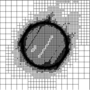
(b) Adaptive mesh for target quantity (5.2) with 56222 degrees of freedom.

Figure 5.1: Comparison of $L^{2}$-errors and visualization of the adaptive mesh for Example 5.1.

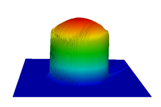
(a) Global Refinement.

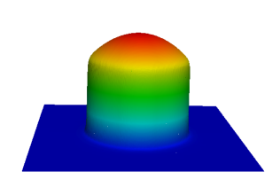
(b) Adaptive Refinement.

Figure 5.2: Stabilized solution profile on a globally refined mesh with 66049 degrees of freedom (5.2a) and on an adaptively refined mesh with error control by the target quantity (5.2) with 56222 degrees of freedom (5.2b) for Example 5.1.

In Fig. 5.3 we present the calculated effectivity indices (4.3) for solving the primal and dual problem in different pairs of finite element spaces based on the $Q_{k}$ element of polynomials of maximum degree $k$ in each variable. Considering the $Q_{1}$ based approximation of the primal problem, we note that by increasing the polynomial degree of the dual solution from $Q_{2}$ to $Q_{4}$ the mesh adaptation process reaches the stopping criterion faster and requires less degrees of freedom. This observation is reasonable, since a higher order approximation of the dual problem is closer to its exact solution of the dual problem, which is part of the error representation (3.20). Thus we conclude that a better approximation of the weights provides a higher accuracy of the error estimator. This observation is also confirmed by the pairs of $Q_{2}/Q_{3}$ with $Q_{2}/Q_{4}$ based finite element spaces. Nevertheless, the difference for using higher-order finite elements for solving the dual problem is not that significant, even less if we take into account the higher computational costs for solving the algebraic form of the dual problem for an increasing order of the piecewise polynomials. Using pairs of $Q_{k}/Q_{k+1}$ based elements for the approximation of the primal and dual problem, the error estimator gets worse for increasing values of the parameter $k$. This observation is in good agreement with the results in [18, Example 3]. A reason for this behavior is given by the observation that for increasing values of $k$ the mesh is less refined for the same number of degrees of freedom. Therefore less cells are available to capture the strong gradients of the exact solution. This argues for choosing smaller values of $k$ in the application of our DWR based approach.

Figure 5.3: Effectivity indices over degrees of freedom for the target quantity (5.2) and different polynomial degrees for Example 5.1.

5.2 Example 2 (Point-value error control, 2d).

In this example we study the application of our approach for different target functionals and a sequence of decreasing diffusion coefficients. Thereby we aim to analyze the robustness of the approach with respect to the small perturbation parameter $\varepsilon$ in (2.1). If convection-dominated problems are considered, or also often for applications of practical interest, local quantities are of greater interest than global ones. The DWR approach offers the appreciable advantage over standard a posteriori error estimators that an error control in an arbitrary user-chosen quantity and not only in the global $L^{2}$ norm, as in Example 1, or a norm of energy type can be obtained. Since the error representation is exact up to higher order terms (cf. Thm. 3.5), robustness with respect to the perturbation parameter $\varepsilon$ can be expected to be feasible. Of course, the approximation of the dual solution $z$ in (3.20) adds a source of uncertainty in the error representation. In the sequel, we evaluate the potential of our approach with respect to these topics for different target functionals. As a benchmark problem we consider problem (2.1) for the solution (cf. [29, Example 4.2])

$$u(\boldsymbol{x})=\frac{1}{2}\left(1-\operatorname{tanh}\frac{2x_{1}-x_{2}-0.25}{\sqrt{5\varepsilon}}\right)$$ (5.3)

with corresponding right-hand side function $f$. Further, $\Omega=(0,1)^{2}$, $\alpha=1.0$, $\boldsymbol{b}=\frac{1}{\sqrt{5}}(1,2)^{\top}$. The Dirichlet boundary condition is given by the exact solution. The solution is characterized by an interior layer of thickness $\mathcal{O}(\sqrt{\varepsilon}|\operatorname{ln}\varepsilon|)$. We study the target functionals

$$J_{L^{2}}(u)=\frac{1}{\|e\|_{L^{2}(\Omega)}}(e,u)_{\Omega}\,,\qquad J_{1}(u)=\int_{\Omega}u\,\mathrm{d}\boldsymbol{x}\qquad\mbox{and}\qquad J_{2}(u)=u(\boldsymbol{x}_{e})\,,$$

where $e:=u-u_{h}$ and with a user-prescribed control point $\boldsymbol{x}_{e}=\left(\frac{5}{16},\frac{3}{8}\right)$ that is located in the interior of the layer. In our computations we regularize $J_{2}(\cdot)$ by

$$J_{r}(u)=\frac{1}{|B_{r}|}\int_{B_{r}}u(\boldsymbol{x})\,\mathrm{d}\boldsymbol{x}\,,$$

where the ball $B_{r}$ is defined by $B_{r}=\left\{\boldsymbol{x}\in\Omega\mid\|\boldsymbol{x}-\boldsymbol{x}_{e}\|<r\right\}$ with small radius $r>0$.

Here, all test cases are solved by using the $Q_{1}/Q_{2}$ pair of finite elements for the primal and dual problem which is due to the observations depicted in Example 1. In Table 5.1 and Fig. 5.4 we present the effectivity indices of the proposed DWR approach applied to the stabilized approximation scheme (2.14) for a sequence of vanishing diffusion coefficients. For the target functionals $J_{L^{2}}(\cdot)$ and $J_{1}(\cdot)$ the effectivity indices nicely converge to one for an increasing number of degrees of freedom. Moreover, the expected convergence behavior is robust with respect to the small diffusion parameter $\varepsilon$. For the more challenging error control of a point-value, which however can be expected to be of higher interest in practice, the effectivity indices also convergences nicely to one. This is in good agreement with effectivity indices for point-value error control that are given in other works of the literature for the pure Poisson problem; cf. [6, p. 45]. We note that in the case of a point-value error control the target functional lacks the regularity of the right-hand side term in the dual problem that is typically needed to ensure the existence and regularity of weak solutions; cf. [19, Chapter 6.2]. However, no impact of this lack of regularity is observed in the computational studies. Thus, for all target functionals a robust convergence behavior is ensured for this test case.

$\varepsilon=10^{-6}$						$\varepsilon=10^{-7}$						$\varepsilon=10^{-8}$
$J_{L^{2}}$		$J_{1}$		$J_{r}$		$J_{L^{2}}$		$J_{1}$		$J_{r}$		$J_{L^{2}}$		$J_{1}$		$J_{r}$
dofs	$\mathcal{I}_{\mathrm{eff}}$	dofs	$\mathcal{I}_{\mathrm{e}ff}$	dofs	$\mathcal{I}_{\mathrm{e}ff}$	dofs	$\mathcal{I}_{\mathrm{eff}}$	dofs	$\mathcal{I}_{\mathrm{e}ff}$	dofs	$\mathcal{I}_{\mathrm{e}ff}$	dofs	$\mathcal{I}_{\mathrm{eff}}$	dofs	$\mathcal{I}_{\mathrm{e}ff}$	dofs	$\mathcal{I}_{\mathrm{e}ff}$
4531	0.72	5355	0.14	4334	1.09	1643	0.32	4034	0.12	753	0.73	1477	0.46	2810	0.56	1841	1.00
7603	0.84	9458	1.92	6468	1.16	2772	0.37	8383	6.38	1841	0.99	5668	0.54	10925	0.90	3301	1.22
13319	0.92	16067	1.73	13851	1.58	5094	0.43	16314	0.01	6358	1.34	10005	0.56	22028	0.05	6411	1.46
24418	0.98	28584	0.85	19670	1.19	10086	0.53	28310	0.13	12674	1.23	17974	0.59	41088	1.72	12904	1.72
42174	1.00	52024	3.06	38002	0.99	21071	0.67	44111	0.61	25558	1.09	41402	0.66	71646	0.26	27039	1.74
76341	1.01	95006	1.07	51603	1.20	46172	0.84	72705	1.07	54549	0.96	90486	0.78	141031	1.96	58254	1.46
126757	0.99	179893	1.01	119171	0.94	103077	0.97	178757	0.85	139531	1.31	253203	0.90	305855	1.01	123436	1.24
224160	1.01	307864	1.00	357046	0.90	240672	1.02	433232	1.00	387749	1.27	502287	1.00	608497	1.04	274188	1.13
409008	0.99	560046	1.00	571577	1.14	580812	1.00	1003495	1.00	1181627	1.01	801381	1.01	856320	1.01	691860	1.08

Table 5.1: Effectivity indices for the target quantities $J_{L^{2}}$  $J_{1}$ and $J_{r}$ and different decreasing perturbation parameters for Example 5.2.

Figure 5.4: Effectivity indices over degrees of freedom for different target functionals and decreasing diffusion coefficient for Example 5.2.

For completeness, in Figure 5.5 we visualize the computed solution profiles and adaptive meshes for an error control based on the local target functional $J_{r}(\cdot)$ and the global target functional $J_{L^{2}}(\cdot)$, respectively. This test case nicely illustrates the potential of the DWR approach. For the point-value error control the refined mesh cells are located close to the specified point of interest and along those cells that affect the point-value error by means of transport in the direction of the flow field $\boldsymbol{b}$. Furthermore, the mesh cells without strong impact on the solution close to the control point are coarsened further. Even though a rough approximation of the sharp interface is obtained in downstream direction from the viewpoint of the control point, in its neighborhood an excellent approximation of the sharp layer is ensured by the approach. A highly economical mesh along with a high quality in the computation of the user-specified goal quantity is thus obtained. In contrast to this, the global error control of $J_{L^{2}}(\cdot)$ provides a good approximation of the solution in the whole domain by adjusting the mesh along the complete layer.

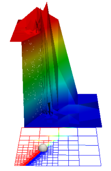
(a) Point-value error control.

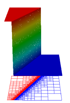
(b) Global error control.

Figure 5.5: Point-value error control by $J_{2}$ (5.5a) and global error control by $J_{L^{2}}$ (5.5b) by the DWR approach for Example 5.2.

5.3 Example 3 (Variable convection field, 3D).

In our last test case we apply the approach to a three-dimensional test case which represents a more challenging task. Moreover, we consider a velocity field $\boldsymbol{b}$ depending on the space variable $\boldsymbol{x}$. Precisely, we consider problem (2.1) with the unit cube $\Omega=(0,1)^{3}$, $\varepsilon=10^{-6}$, $\alpha=1$, $\boldsymbol{b}=(-x_{2},x_{1},0)^{\top}$ and $f\equiv 0$. The boundary conditions are given by $\frac{\partial u}{\partial\boldsymbol{n}}=0$ on $\Gamma_{N}=\{\boldsymbol{x}~{}\in~{}\Omega\mid x_{1}=0\}$, $u=1$ on $\Gamma_{D_{1}}=\{\boldsymbol{x}\in\Omega\mid 0.4\leq x_{1}\leq 0.6,x_{2}=0,0.4\leq x_{3}\leq 0.6\}$, and $u=0$ on $\Gamma_{D_{2}}=\partial\Omega\backslash\{\Gamma_{N}\cup\Gamma_{D_{1}}\}$. Thus, by the boundary part $\Gamma_{D_{1}}$ we model an inflow region (area) where the transport quantity modelled by the unknown $u$ is injected; cf. Fig. 5.6. $\Gamma_{N}$ models an outflow boundary. Prescribing a homogeneous Dirichlet condition on $\Gamma_{D_{2}}$ is done for the sake of simplicity and of no real relevance for the test setting. The target functional aims at the control of the solution’s mean value in a smaller, inner domain $\Omega_{In}=[0,0.1]\times[0.4,0.6]\times[0.4,0.6]$, and is given by

$$J_{4}(u)=\int_{\Omega_{In}}u\,\mathrm{d}\boldsymbol{x}\,.$$

In the context of applications, the transport quantity $u$ is thus measured and controlled in the small region of interest $\Omega_{In}$.

Figure 5.6 illustrates the computed adaptively generated meshes for some of the DWR iteration steps. For visualization purposes, two surfaces with corresponding mesh distribution are shown for each grid, the bottom surface and the surface in the domain’s center with respect to the $x_{3}$ direction. We note that the postprocessed solutions are visualized on a grid for the respective surfaces. The cells on the surfaces are triangular-shaped since the used visualization software ParaView is based on triangular-shaped elements. Similar to the previous test case of a point-value error control, the refinement is located on those cells that affect the mean value error control. Here, the cells close to the two inner layers aligned in the flow direction $\boldsymbol{b}$ are strongly refined. This refinement process is obvious since the inner and control domain $\Omega_{In}$ is chosen to have exactly the same dimensions as the channel-like extension of the boundary segment $\Gamma_{D_{1}}$ along the flow direction into the domain $\Omega$. Outside the inner domain $\Omega_{In}$ and the channel-like domain of transport the mesh cells are coarsened for an increasing number of DWR iteration steps.

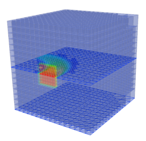
(a)

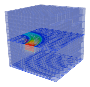
(b)

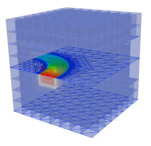
(c)

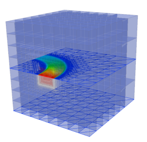
(d)

Figure 5.6: Adaptive grids after first (5.6a), third (5.6b), fifth (5.6c) and seventh (5.6d) iteration step of the DWR approach with coarsening and refinement with target functional $J_{1}$ for Example 5.3.

6 Summary

In this work we developed an adaptive approach for stabilized finite element approximations of stationary convection-dominated problems. It is based on the Dual Weighted Residual method for goal-oriented a posteriori error control. A first dualize and then stabilize philosophy was applied for combining the mesh adaptation process in the course of the DWR approach with the stabilization of the finite element techniques. In contrast to other works of the literature we used a higher order approximation of the dual problem instead of a higher order interpolation of a lower order approximation of the dual solution. Thereby we aim to eliminate sources of inaccuracies in regions with layers and close to sharp fronts. In numerical experiments we could prove that spurious oscillations that typically arise in numerical approximations of convection-dominated problems could be reduced significantly. Robust effectivity indices very close to one were obtained for the specified test target quantities. We demonstrated the efficiency of the approach also for three space dimensions. The presented approach offers large potential for combining goal-oriented error control and selfadaptivity with stabilized finite element methods in the approximation of convection-dominated transport. The application of the approach to nonlinear, nonstationary and more sophisticated problems of multiphysics is our ongoing work. Moreover, the efficient computation of the higher order approximation to the dual problem offers potential for optimization. This will also be our work for the future.

References

- [1] Ahmed, N., John, V.: Adaptive time step control for higher order variational time discretizations applied to convection-diffusion equations. Comput. Methods Appl. Mech. Engrg. 285, 83–101 (2015)
- [2] Angermann, L.: Balanced a posteriori error estimates for finite-volume type discretizations of convection-dominated elliptic problems. Computing. 55(4), 305–323 (1995)
- [3] Arndt, D., Bangerth, W., Davydov, D., Heister, T., Heltai, L., Kronbichler, M., Maier, M., Pelteret, J.-P., Turcksin, B., Wells, D.: The deal.II Library, Version 8.5. J. Numer. Math. 25(3), 137–146 (2017). doi:10.1515/jnma-2016-1045
- [4] Bangerth, W., Geiger, M., Rannacher, R.: Adaptive Galerkin finite element methods for the wave equation. Comput. Methods Appl. Math. 10, 3–48 (2010)
- [5] Bangerth, W., Hartmann, R., Kanschat, G.: deal.II-A general purpose object oriented finite element library. ACM Trans. Math. Software 33(4), 24/1–24/27 (2007). doi:10.1145/1268776.1268779
- [6] Bangerth, W., Rannacher, R.: Adaptive Finite Element Methods for Differential Equations. Birkhäuser, Basel (2003)
- [7] Barrenechea, G. R., John, V., Knobloch, P.: Analysis of algebraic flux correction schemes. SIAM J. Numer. Anal. 54(4), 2427–2451 (2016)
- [8] Bause, M., Köcher, U.: Variational time discretization for mixed finite element approximations of nonstationary diffusion problems. J. Comput. Appl. Math. 289, 208–224 (2015)
- [9] Bause, M., Schwegler, K.: Analysis of stabilized higher order finite element approximation of nonstationary and nonlinear convection-diffusion-reaction equations. Comput. Methods Appl. Mech. Engrg. 209–212, 184–196 (2012)
- [10] Becker, R.: An optimal-control approach to a posteriori error estimation for finite element discretizations of the Navier–Stokes equations, East-West J. Numer. Math. 8, 257–274 (2000)
- [11] Becker, R., Rannacher, R.: Weighted a posteriori error control in FE methods. In: Bock, H. G. et al. (eds.) ENUMATH 97. Proceedings of the 2nd European Conference on Numerical Mathematics and Advanced Applications, pp. 621–637. World Scientific, Singapore (1998)
- [12] Becker, R., Rannacher, R.: An optimal control approach to a posteriori error estimation in finite element methods. Acta Numer. 10, 1–102 (2001)
- [13] Brooks, A. N., Hughes, T. J. R.: Streamline upwind/Petrov-Galerkin formulations for convection dominated flows with particular emphasis on the incompressible Navier-Stokes equations. Comput. Methods Appl. Mech. Engrg. 32(1-3), 199–259 (1982)
- [14] Carey, G. F., Oden, J. T.: Finite Elements, Computational Aspects, Vol. III (The Texas finite element series). Prentice-Hall, Englewood Cliffs, New Jersey (1984)
- [15] Ciarlet, P. G.: Basic error estimates for elliptic problems. In: Ciarlet, P. G., Lions, J. L. (eds.) Handbook of Numerical Analysis, vol. 2, pp. 17-351, North-Holland, Amsterdam (1991)
- [16] Dolejší, V., Ern, A., Vohralkík, M.: A framework for robust a posteriori error control in unsteady nonlinear advection-diffusion problems. SIAM J. Numer. Anal. 51(2), 773–793 (2013)
- [17] Dörfler, W.: A convergent adaptive algorithm for Poisson’s equation. SIAM J. Numer. Anal. 33, 1106–1124 (1996)
- [18] Endtmayer, B., Wick, T.: A partition-of-unity dual-weighted residual approach for multi-objective goal functional error estimation applied to elliptic problems. Comput. Methods Appl. Math. 17(4), published online (2017). doi:10.1515/cmam-2017-0001
- [19] Evans, L. C.: Partial Differential Equations. American Mathematical Society, Providence, Rhode Island (2010)
- [20] Hughes, T. J. R., Brooks, A. N.: A multidimensional upwind scheme with no crosswind diffusion. In: Hughes, T. J. R. (eds.) Finite Element Methods for Convection Dominated Flows, AMD, vol. 34, pp. 19–35. Amer. Soc. Mech. Engrs. (ASME) (1979)
- [21] Hughes, T. J. R., Mallet, M., Mizukami, A.: A new finite element formulation for computational fluid dynamics: II. Beyond SUPG. Comput. Methods Appl. Mech. Engrg. 54, 341–355 (1986)
- [22] John, V., Knobloch, P.: Adaptive computation of parameters in stabilized methods for convection-diffusion problems. In: Cangiani, A. et al. (eds.) Numerical Mathematics and Advanced Applications 2011, Springer, Heidelberg (2013)
- [23] John, V., Knobloch, P., Savescu, S. B.: A posteriori optimization of parameters in stabilized methods for convection-diffusion problems - Part I. Comput. Methods Appl. Mech. Engrg. 200, 2916–2929 (2011)
- [24] John, V., Novo, J.: A robust SUPG norm a posteriori error estimator for stationary convection-diffusion equations. Comput. Methods Appl. Mech. Engrg. 255, 289–305 (2013)
- [25] John, V., Schmeyer, E.: Finite element methods for time-dependent convection-diffusion-reaction equations with small diffusion Comput. Methods Appl. Mech. Engrg. 198, 475–494 (2008)
- [26] Köcher, U.: Variational space-time methods for the elastic wave equation and the diffusion equation, Dissertation, Helmut Schmidt University Hamburg, urn:nbn:de:gbv:705-opus-31129, 2015.
- [27] Köcher, U, Bruchhäuser, M. P., Bause, M.: Efficient and scaleable data structures and algorithms for goal-oriented adaptivity of space–time FEM codes. In progress, 1–6 (2018).
- [28] Kuzmin, D., Löhner, R., Turek, S.: Flux-Corrected Transport: Principles, Algorithms, and Applications. Springer, Berlin (2012)
- [29] Lube, G., Rapin, G.: Residual-based stabilized higher-order FEM for advection-dominated problems. Comput. Methods Appl. Mech. Engrg. 195, 4124–4138 (2006)
- [30] Roos, H.-G., Stynes, M., Tobiska, L.: Robust Numerical Methods for Singularly Perturbed Differential Equations. Springer, Berlin (2008)
- [31] Schwegler, K.: Adaptive goal-oriented error control for stabilized approximations of convection-dominated problems, Dissertation, Helmut Schmidt University Hamburg, http://edoc.sub.uni-hamburg.de/hsu/volltexte/2014/3086/, 2014.
- [32] Verfürth, R.: A posteriori error estimation techniques for finite element methods. Oxford University Press, Oxford (2013)