On the importance of the nonequilibrium ionization of Si IV and O IV and the line-of-sight in solar surges

Abstract

Surges are ubiquitous cool ejections in the solar atmosphere that often appear associated with transient phenomena like UV bursts or coronal jets. Recent observations from the Interface Region Imaging Spectrograph (IRIS) show that surges, although traditionally related to chromospheric lines, can exhibit enhanced emission in Si IV with brighter spectral profiles than for the average transition region (TR). In this paper, we explain why surges are natural sites to show enhanced emissivity in TR lines. We performed 2.5D radiative-MHD numerical experiments using the Bifrost code including the nonequilibrium ionization of silicon and oxygen. A surge is obtained as a by-product of magnetic flux emergence; the TR enveloping the emerged domain is strongly affected by nonequilibrium effects: assuming statistical equilibrium would produce an absence of Si IV and O IV ions in most of the region. Studying the properties of the surge plasma emitting in the Si IV 1402.77 Å and O IV 1401.16 Å lines, we find that a) the timescales for the optically-thin losses and heat conduction are very short, leading to departures from statistical equilibrium, and b) the surge emits in Si IV more and has an emissivity ratio of Si IV to O IV larger than a standard TR. Using synthetic spectra, we conclude the importance of line-of-sight effects: given the involved geometry of the surge, the line-of-sight can cut the emitting layer at small angles and/or cross it multiple times, causing prominent, spatially intermittent brightenings both in Si IV and O IV.

1 Introduction

The solar atmosphere contains a wide variety of chromospheric ejections that cover a large range of scales: from the smallest ones with maximum size of a few megameters, such as penumbral microjets (e.g., Katsukawa et al., 2007; Drews & Rouppe van der Voort, 2017), or spicules (Hansteen et al., 2006; De Pontieu et al., 2007; Pereira et al., 2012, among others); up to ejections that can reach, in extreme cases, several tens of megameters, like surges (e.g., Canfield et al., 1996; Kurokawa et al., 2007; Guglielmino et al., 2010; Yang et al., 2014) and macrospicules (Bohlin et al., 1975; Georgakilas et al., 1999; Murawski et al., 2011; Kayshap et al., 2013). Surges, in particular, are often associated with magnetic flux emergence from the solar interior. They are typically observed as darkenings in images taken in the H$\alpha$ blue/red wings with line-of-sight (LOS) velocities of a few to several tens of km s^-1, and are usually related to other explosive phenomena like EUV and X-ray jets, UV bursts and Ellerman bombs (see Nóbrega-Siverio et al., 2017, hereafter NS2017, and references therein). Although observationally known for several decades now, the understanding of surges has progressed slowly and various aspects like, e.g., their impact on the transition region (TR) and corona concerning the mass and energy budget, are still poorly known.

From the theoretical point of view, the first explanation of the surge phenomenon came through 2.5D numerical models (Shibata et al., 1992; Yokoyama & Shibata, 1995, 1996), where a cold ejection was identified next to a hot jet as a consequence of a magnetic reconnection process between the magnetic field in plasma emerged from the interior and the preexisting coronal field. Nishizuka et al. (2008) used a similar numerical setup to associate the surge with jet-like features seen in Ca II H+K observations by means of morphological image comparisons. Further 2.5D models that include the formation of a cool chromospheric ejection are those of Jiang et al. (2012) (canopy-type coronal magnetic field), and Yang et al. (2013, 2018), who study the cool jets resulting from the interaction between moving magnetic features at the base of their experiment and the preexisting ambient field in the atmosphere. Turning to three dimensional models, in the magnetic flux emergence experiment of Moreno-Insertis & Galsgaard (2013), a dense wall-like surge appeared surrounding the emerged region with temperatures from $10^{4}$ K to a few times $10^{5}$ K and speeds around $50$ km s^-1. MacTaggart et al. (2015) found similar velocities for the surges in their 3D model of flux emergence in small-scale active regions. The availability of a radiation-MHD code like Bifrost (Gudiksen et al., 2011) has opened up the possibility of much more detailed modeling of the cool ejections than before. Bifrost has a realistic treatment of the material properties of the plasma, calculates the radiative transfer in the photosphere and chromosphere and includes the radiative and heat conduction entropy sources in the corona. Using that code, Nóbrega-Siverio et al. (2016), hereafter NS2016, argued that entropy sources play an important role during the surge formation and showed that a relevant fraction of the surge could not be obtained in previous and more idealized experiments.

The realistic treatment of surges may require an even larger degree of complication. The solar atmosphere is a highly dynamical environment; the evolution sometimes occurs on short timescales that bring different atomic species out of equilibrium ionization, thus complicating both the modeling and the observational diagnostics (e.g., Griem, 1964; Raymond & Dupree, 1978; Joselyn et al., 1979; Hansteen, 1993). For hydrogen, for instance, using 2D numerical experiments, Leenaarts et al. (2007, 2011) found that the temperature variations in the chromosphere can be much larger than for statistical equilibrium (SE), which has an impact on, e.g., its coolest regions (the so-called cool pockets). For helium, Golding et al. (2014, 2016) described how nonequilibrium (NEQ) ionization leads to higher temperatures in wavefronts and lower temperatures in the gas between shocks. For heavy elements, Bradshaw & Mason (2003); Bradshaw & Cargill (2006); Bradshaw & Klimchuk (2011); Reep et al. (2016) showed, through 1D hydrodynamic simulations, that there are large departures from SE balance in cooling coronal loops, nanoflares and other impulsive heating events that affects the EUV emissivity. Through 3D experiments, Olluri et al. (2013a) found that deduced electron densities for O IV can be up to an order of magnitude higher when NEQ effects are taken into account. Also in 3D, Olluri et al. (2015) discussed the importance of the NEQ ionization of coronal and TR lines to reproduce absolute intensities, line widths, ratios, among others, observed by, e.g., Chae et al. (1998); Doschek (2006); Doschek et al. (2008). De Pontieu et al. (2015) were able to explain the correlation between non-thermal line broadening and intensity of TR lines only when including NEQ ionization in their 2.5D numerical experiments. Martínez-Sykora et al. (2016) studied the statistical properties of the ionization of silicon and oxygen in different solar contexts: quiet Sun, coronal hole, plage, quiescent active region, and flaring active region, finding similarities with the observed intensity ratios only if NEQ effects are taken into account. Given their highly time-dependent nature and the relevance of the heating and cooling mechanisms in their evolution, surges are likely to be affected by NEQ ionization. Motivated by this fact, NS2017 included the NEQ ionization of silicon to compare synthetic Si IV spectra of two 2.5D numerical experiments with surge observations obtained by the Interface Region Imaging Spectrograph (IRIS, De Pontieu et al., 2014) and the Swedish 1-m Solar Telescope (SST, Scharmer et al., 2003). The results showed that the experiments were able to reproduce major features of the observed surge; nonetheless, the theoretical aspects to understand the enhanced Si IV emissivity within the numerical surge and its properties were not addressed in that publication.

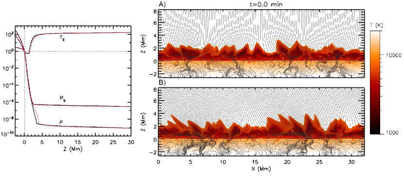
Figure 1: Left: Horizontal averages for the initial stratification of $\rho$, $P_{g}$, and $T$ normalized to their photospheric values at $z=0$ Mm, namely, $\rho_{ph}=3.1\times 10^{-7}$ g cm^-3, $P_{g_{ph}}=1.1\times 10^{5}$ erg cm^-3 and $T_{ph}=5.7\times 10^{3}$  K. Solid black line represents the stratification for the vertical coronal field experiment; the red dotted, for the slanted one. The horizontal and vertical dotted lines mark the reference normalization values at $z=0$ Mm. Right: 2D maps for the initial temperature with magnetic field lines in black for the vertical experiment (top) and slanted experiment (bottom). The maps only show temperatures below $2\times 10^{4}$ K (although the range varies from 1660 K up to $\sim$ 1 MK) and heights between $-2.6\leq z\leq 8.0$ Mm (the top of the domain reaches $z=30$ Mm). The solar surface is roughly at $z=0$ Mm (white dashed horizontal line).

The aim of the present paper is to provide theoretical explanations concerning the relevance of the NEQ ionization for surges and the corresponding impact on the emissivity of TR lines. We use 2.5D numerical experiments carried out with the Bifrost code (Gudiksen et al., 2011) including the module developed by Olluri et al. (2013b) that solves the time-dependent rate equations to calculate the ionization states of different elements, thus allowing for departures from SE. Here we apply this module to determine the ionization levels of silicon and oxygen. We conclude that consideration of NEQ is necessary to get the proper population levels of the ions and, consequently, the right emissivity to interpret observations. A statistical analysis of temperature is provided to constrain the plasma properties involved in the emissivity of relevant lines of Si IV and O IV within the surges. Through detailed Lagrange tracing, we are able to determine the origin of the emitting plasma and the role of the optically thin radiation and thermal conduction to explain the departure of SE of the relevant ions. Furthermore, we compute synthetic profiles to understand previous observational results and predict future ones, highlighting the surge regions that are more likely to be detected and addressing the importance of the angle of LOS.

The layout of the paper is as follows. Section 2 describes the physical and numerical models. Section 3 explains the general features of the time evolution of the experiments. In Section 4, we show the main results of the paper splitting the section in a) the relevance of the NEQ ionization of Si IV , and also O IV, in surges (Section 4.1); b) the consequences of the NEQ ionization for the surge plasma emitting in those TR lines, analyzing its properties and compare them with a generic quiet TR (Section 4.2); and c) the origin of the NEQ plasma, addressing the role of the entropy sources (Section 4.3). In Section 5, we have calculated absolute intensities and synthetic spectral profiles for diagnostic purposes and comparison with observations, emphasizing also the importance of the surge geometry and LOS. Finally, Section 6 contains a summary and conclusions.

2 The physical and numerical model

We have run two 2.5D numerical flux emergence experiments in which surges are a natural consequence of magnetic reconnection processes. Those two experiments were also used by NS2017 and Rouppe van der Voort et al. (2017) to compare the synthetic profiles with the complex profiles observed with IRIS and SST.

This section is divided into two parts: (1) the numerical code, and (2) the description of the model underlying our experiments.

2.1 The numerical code

The two experiments have been carried out with the 3D radiation-MHD (R-MHD) Bifrost code (Gudiksen et al., 2011; Carlsson & Leenaarts, 2012; Hayek et al., 2010), which treats the radiative transfer from the photosphere to the corona and thermal conduction in a self-consistent manner (see also NS2016 for further details of this code applied to surge experiments). Furthermore, we have enabled in the code a module developed by (Olluri et al., 2013b) to follow the NEQ ionization states of elements with atomic number greater than 2. This module solves the rate equations for those elements using the temperature, mass density, electronic number density $n_{e}$ and velocity values of the simulation without modifying the results of the R-MHD calculation, so there is no feedback, e.g., on the energy equation terms such as the optically thin losses (see the discussion in Section 6.1). In particular, we have employed it to calculate the NEQ ionization fraction for silicon and oxygen, using abundances from Asplund et al. (2009), 7.52 and 8.69, respectively, in the customary astronomical scale where 12 corresponds to hydrogen.

2.2 Description of the models

2.2.1 Physical domain and initial condition

In the two experiments, we began with a statistically stationary 2D snapshot that spans from the uppermost layers of the solar interior to the corona, and whose physical domain is $0.0$ Mm $\leq x\leq$ $32.0$ Mm and $-2.6$ Mm $\leq z\leq$ $30.0$ Mm, where $z=0$ Mm corresponds to the solar surface. The grid is uniform in the $x$-direction with $\Delta x=31$ km, but it is nonuniform in the vertical direction in order to better resolve the photosphere and chromosphere: the vertical grid spacing is $20$ km from the photosphere to the transition region, and increases gradually in the corona up to $147$ km at the top of the domain.

The left panel in Figure 1 contains the horizontal averages for the initial density, $\rho$, gas pressure, $P_{g}$, and temperature, $T$, for both experiments normalized to photospheric values, namely, $\rho_{ph}=3.1\times 10^{-7}$ g cm^-3, $P_{g_{ph}}=1.1\times 10^{5}$ erg cm^-3 and $T_{ph}=5.7\times 10^{3}$  K. The corona has a temperature around $1$ MK and a magnetic field with a strength of $10$ G, with the difference that one of the experiments (hereafter the vertical experiment) has a vertical magnetic field in the corona while in the other (the slanted experiment), the magnetic field in the corona is inclined $30$° with respect to the vertical direction (see magnetic field lines superimposed in black in the 2D temperature maps for the initial snapshot in Figure 1).

2.2.2 Chemical elements calculated in NEQ and their spectral lines

We have used the NEQ module of Olluri et al. (2013b) mentioned in the Introduction to compute the nonequilibrium ionization of silicon in both numerical experiments. Furthermore, in the vertical experiment we also calculate the NEQ ionization of oxygen, with the goal of predicting future observational results. Once the NEQ populations are obtained, we are able to compute the emissivity using

$$\epsilon_{\lambda} = \frac{h\,c}{4\,\pi\,\lambda}\,n_{u}\,A_{ul},$$ (1)

where $h$ is the Planck’s constant, $c$ the light speed, $\lambda$ is the wavelength of the spectral line, $n_{u}$ the population density of the upper level of the transition (i.e., the number density of emitters), and $A_{ul}$ the Einstein coefficient for spontaneous de-excitation given by

$$A_{ul} = \frac{8\,\pi^{2}\,e^{2}\,}{m_{e}\,c}\frac{1}{\lambda^{2}}\,\frac{g_{l}}{g_{u}}\,f_{lu},$$ (2)

where $e$ is the electron charge, $m_{e}$ the electron mass, $g_{l}$ and $g_{u}$ the statistical weights of the lower and upper states respectively, and $f_{lu}$ the oscillator strength. The units used in this paper for the emissivity $\epsilon$ are erg cm^-3 sr^-1 s^-1. For the sake of compactness, we will refer to it in the following as $\epsilon_{{}_{CGS}}$.

Since we are interested in understanding the response of the TR to chromospheric phenomena like surges, we have chosen the following IRIS lines: Si IV 1402.77 Å, which is the weakest of the two silicon resonance lines; and O IV 1401.16 Å, the strongest of the forbidden oxygen lines that IRIS is able to observe. The corresponding formation temperature peaks in statistical equilibrium, $T_{{}_{SE}}$, and other relevant parameters to calculate the Einstein coefficient (Equation 2) and the corresponding emissivity (Equation 1) of these lines are shown in Table 1. Under optically thin conditions, Si IV 1393.76 Å is twice stronger than 1402.77 Å, so the results we obtain in this paper can also be applied to Si IV 1393.76 Å. Furthermore, the study of Si IV 1402.77 Å can provide theoretical support to our previous paper NS2017. In turn, the choice of the 1401.16 Å line for oxygen is because the O IV lines are faint and require longer exposure times to be observed (De Pontieu et al., 2014). Thus, in order to make any prediction that could be corroborated in future IRIS analysis, we focus on the strongest of the oxygen lines, which has a better chance to be detected. For simplicity, hereafter we refer to the Si IV 1402.77 Å and O IV 1401.16 Å emissivities as the Si IV and O IV emissivities, respectively.

Table 1: Relevant parameters for the studied emission lines

Line	$T_{{}_{SE}}$ (K)	$g_{u}$	$g_{l}$	$f_{lu}$	$n_{u}/\epsilon_{\lambda}$
Si IV 1402.77 Å	$10^{4.9}$	$2$	$2$	$2.7\times 10^{-1}$	$974$
O IV 1401.16 Å	$10^{5.2}$	$6$	$4$	$5.1\times 10^{-7}$	$7.62\times 10^{8}$

2.2.3 Boundary conditions

We are imposing periodicity at the side boundaries; for the vertical direction, characteristic conditions are implemented at the top, whereas an open boundary is maintained at the bottom keeping a fixed value of the entropy of the incoming plasma. Additionally, in order to produce flux emergence, we inject a twisted magnetic tube through the bottom boundary following the method described by Martínez-Sykora et al. (2008). The parameters of the tube (specifically, the initial location of the axis, $x_{0}$ and $z_{0}$; the field strength there, $B_{0}$; the tube radius $R_{0}$; and the amount of field line twist $q$) are identical in both experiments and given in Table 2.2.3. The total axial magnetic flux is $\Phi_{0}=6.3\times 10^{18}$ Mx, which is in the range of an ephemeral active region (Zwaan, 1987). Details about this kind of setup are provided in the paper by NS2016.

Table 2: Parameters of the initial twisted magnetic tube for both experiments

$x_{0}$ (Mm)	$z_{0}$ (Mm)	$R_{0}$ (Mm)	$q$ (Mm-1)	$B_{0}$ (kG)
15.0	-2.8	0.10	2.4	20

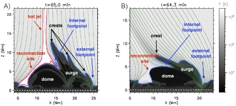
Figure 2: Image (taken from NS2017) showing 2D temperature maps for the context of the surge experiments and the regions of interest. A) The vertical coronal magnetic field experiment at $t=65.0$ minute. B) The slanted coronal magnetic case at $t=64.3$ minute. Additionally, magnetic field lines (green), temperature contours for the $T_{{}_{SE}}=7.9\times 10^{4}$ of Si IV K (blue), and for $T=1.2\times 10^{6}$ K (red) are added.

3 General features of the time evolution of the experiments

The numerical experiments start with the injection of the twisted magnetic tube through the bottom boundary ($t=0$ minute). Within the convection zone, the tube rises with velocities of $\lesssim 2$ km s^-1 and suffers deformations due to the convection flows, mainly in the regions where the downflows are located. The twisted tube continues rising until it reaches the surface. There, the magnetized plasma accumulates until it develops a buoyancy instability ($t\approx 40$ minute) in a similar way as explained by NS2016.

The subsequent phases of evolution are characterized by the emergence and expansion of the magnetized plasma into the solar atmosphere, producing a dome-like structure of cool and dense matter ($t\sim 50$ minute). During the expansion process, the dome interior becomes rarefied due to gravitational flows. Simultaneously, the magnetic field of the emerged plasma collides with the preexisting coronal ambient field and, as a consequence, non-stationary magnetic reconnection occurs, forming and ejecting several plasmoids. Our vertical experiment has recently been used by Rouppe van der Voort et al. (2017) to show that the Si IV spectral synthesis of those plasmoids is able to reproduce the highly broadened line profiles, often with non-Gaussian and triangular shapes, seen in IRIS observations.

As an indirect consequence of the magnetic reconnection, a surge is obtained in both experiments. This is illustrated in Figure 2 through temperature maps with overlying magnetic field lines for each experiment: panel A, the vertical experiment at $t=65.0$ minute, and panel B, the slanted one at $t=64.3$ minute. Those are representative instants when the surge is clearly distinguishable as an elongated structure detached from the dome. For later reference, different regions have been marked in the figure that will be seen below to correspond to prominent features of the surge in terms of NEQ ionization and brightness in the spectra: the internal footpoint, which is located at the base of a wedge created by the detachment process that separates the surge from the dome (NS2016); the external footpoint, which is just the external boundary of the surge, and the flanks and top of the crests. Although not directly discussed in this paper, another region is probably worth mentioning, namely the hot jet: in the vertical experiment, it is shown clearly through the red temperature contour of $T=1.2\times 10^{6}$ K; in the slanted one, the temperatures of the high-speed collimated ejection are not distinguishable from the rest of the corona. The difference between both experiments may be due to the fact that the slanted case has a denser emerged dome and, perhaps, the entropy sources in it are less efficient in heating the plasma that passes through the magnetic reconnection site.

4 The role of the nonequilibrium (NEQ) ionization

The importance of the NEQ ionization is studied in this section from a triple perspective: (a) the comparison of the NEQ number densities with those calculated under the SE approximation (Section 4.1); (b) the consequences for the emissivity of the plasma (Section 4.2); and (c) the key mechanisms that cause the departure from statistical equilibrium in the surge plasma (Section 4.3).

4.1 The SE and NEQ number densities

The results of the current paper are obtained by solving the equation rates for the relevant ionization states of Si and O, i.e., taking into account nonequilibrium effects using the Olluri et al. (2013b) module mentioned in earlier sections: the number densities of emitters $n_{u}$ thus calculated will be indicated with the symbol $n_{{}_{NEQ}}$. In order to test the accuracy of the SE approximation, we have also calculated the $n_{u}$ that would be obtained imposing statistical equilibrium in the Olluri et al. (2013b) module: those will be indicated with the symbol $n_{{}_{SE}}$. The accuracy or otherwise of the SE approximation is measured here through the following ratio:

$$r = \frac{n_{{}_{SE}}-n_{{}_{NEQ}}}{n_{{}_{SE}}+n_{{}_{NEQ}}},$$ (3)

The parameter $r$ varies between -1 and 1; its meaning is as follows:

1. If $r\approxeq 0$, the number density of emitters obtained imposing SE would be approximately equal to the one allowing NEQ rates ($n_{{}_{SE}}\approxeq n_{{}_{NEQ}}$), so in those regions the SE approximation to calculate the state of ionization would be valid.

2. If clearly $r<0$, this means that $n_{{}_{SE}}<n_{{}_{NEQ}}$, so the approximation of SE ionization would underestimate the real population. As $r$ becomes more negative, the NEQ effects would be more prominent and the SE approximation would become less accurate. In the extreme case ($r=-1$), the assumption of SE would mistakenly result in an absence of ions in the ionization state of interest!

3. On the other hand, if $r>0$, it follows that $n_{{}_{SE}}>n_{{}_{NEQ}}$, so the computation of the ionization in SE would be wrong again, but in this case because it would overestimate the real population. When $r=1$, SE would give as a result a totally fictitious population, since the full NEQ calculation indicates that there are no ions!

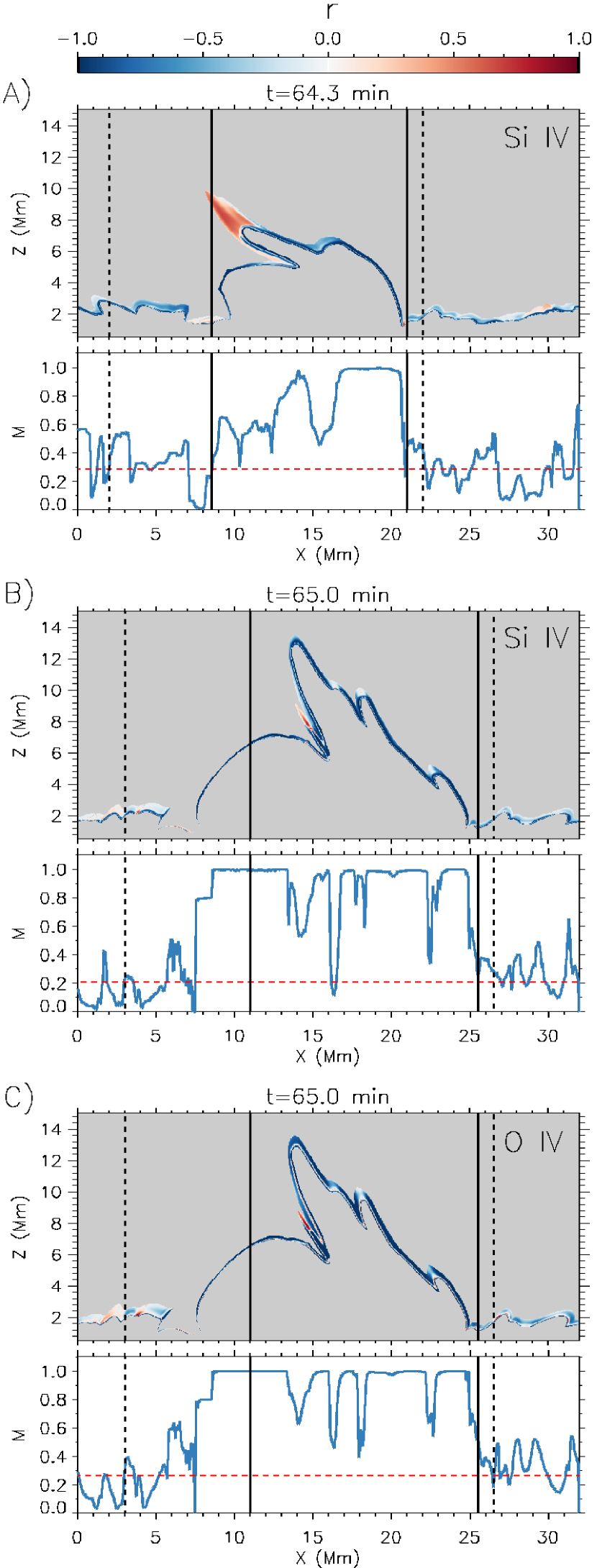
Figure 3: 2D maps of the ratio $r$ from Equation (3) for the Si IV population for (A) the slanted experiment at $t=64.3$ minute and (B) the vertical one at $t=65.0$ minute. Panel C shows $r$ for the O IV population in the vertical experiment at $t=65.0$ minute. A gray color mask is overplotted where the emissivity obtained from the NEQ computation is $\epsilon_{{}_{CGS}}<10^{-10}$. Below each 2D map, the median M of $|r|$ in the high-emissivity region (i.e., outside of the mask) is shown. Solid and dashed vertical lines delimit the ETR and QTR regions, respectively. The horizontal line in the M panels marks the average value of M within the QTR.

The ratio $r$ is plotted in Figure 3 for the two experiments described in this paper. The upper panels in each block contain 2D maps of $r$, namely, for (A) Si IV in the slanted experiment at $t=64.3$ minute; (B) Si IV in the vertical experiment at $t=65$ minute; and (C) O IV also in the vertical experiment at $t=65$ minute. To limit the diagram to the relevant regions, a grey mask is overplotted and only those pixels with emissivity obtained from the NEQ computation above a threshold ($\epsilon_{{}_{CGS}}\geq 10^{-10}$) are being shown. The bottom panel in each block contains a line plot for the median M of the absolute value of $r$ in the regions not covered by the mask in each column. Using the absolute value of the ratio elucidates the areas where NEQ ionization is important, either because SE underestimates ($r<0$) or overestimates ($r>0$) the real number density of emitters $n_{u}$. In the figure, two regions can be clearly distinguished:

1. The Quiet Transition Region (hereafter QTR). We define it as the transition region that has not been perturbed by the flux emergence and subsequent surge and/or jet phenomena. The horizontal extent of the QTR is marked in the figure with dashed vertical lines and corresponds to the region located between $0.0\leq x\leq 2.0$ and $22.0\leq x\leq 32.0$ Mm, for the slanted experiment; and $0.0\leq x\leq 3.0$ and $26.5\leq x\leq 32.0$ Mm, for the vertical one. In this domain, $r$ mostly shows negative values (blue color in the image) in a thin layer in the transition region ($z\sim 2$ Mm). The corresponding M value is on average between $0.2$ and $0.3$ (horizontal dashed line in red in the panels), which indicates that both Si IV and O IV suffer significant departures from statistical equilibrium.

2. The second region corresponds to the main result of this section: the emerged domain, namely, the dome and surge, are severely affected by the NEQ ionization both for silicon and oxygen (see the dark blue color which corresponds to $r\approx-1$, and corresponding M value close to 1). The value $r\approx-1$ is found either in cold regions with $T\sim 2\times 10^{4}$ K and also in hot domains ($T\sim 5\times 10^{5}$ K). Also, on the left of the surge, we also find some regions where $r>0$ (red), especially in the slanted experiment, which indicates that the SE approximation is overestimating the real population. Since our main goal is to study the surge, we focus on its surroundings, and, in particular, on the domain marked in the figure with solid lines, i.e., $8.5\leq x\leq 21.0$ Mm, for the slanted experiment, and $11.0\leq x\leq 25.5$ Mm, for the vertical one. In the following, we refer to this range as the Enhanced Transition Region (ETR). In the associated 1D panels, we see that M shows larger values than in the QTR; in fact, the median reaches values close to one in many places of the ETR . There are some specific locations within the ETR where M shows substantially lower values, e.g., $x=16.2$ Mm or $x=18.1$ Mm in the B and C panels . Looking at the 2D panels, we realize that in those locations, part of the TR has $r$ close to zero (white patch above the blue line). Consequently, the median in that vertical columns decreases. Note, however, that even in those locations the M values in the ETR are larger than, or at least comparable to, the largest ones found in the QTR. This finding highlights the relevance of including the NEQ calculation for eruptive phenomena like surges, since without it, the calculated Si IV and O IV populations would be totally erroneous. This would translate into wrong emissivity values and therefore mistaken synthesis diagnostics.

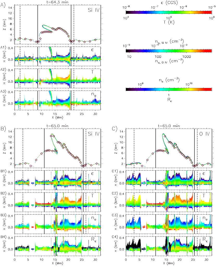
Figure 4: Maps of the 2D emissivity $\epsilon$ for A) Si IV in the slanted experiment, B) Si IV in the vertical one, and C) O IV also for the vertical experiment. Diamonds have been superimposed on the region of high emissivity to mark the position of $z_{max}$ (see Equation 4). A color scale at the right column of the figure contains the translation from emissivity to number densities of emitters $n_{u}$. In each of the blocks, secondary panels for $\epsilon$, $T$, and $n_{e}$ have been inserted that use $H$ as vertical scale. Additionally, a panel of the ratio of the Si IV and O IV emissivities, $R_{\epsilon}$, is added for B and C blocks. All the maps only show places where $\epsilon_{{}_{CGS}}\geq 10^{-8}$. The instants in the panels and the vertical lines are the same as in Figure 3. The accompanying animation shows the time evolution of the three experiments from the early stages of the surge until the its decay phase. (An animation of the figure is available)

4.2 Characterizing the plasma in NEQ

Once we have studied the NEQ effects on the two different domains of our experiments (ETR, QTR), we now turn to the associated question of the emissivity, in particular, for the Si IV and O IV lines. To that end, we start by showing 2D maps of the emissivity in Figure 4 (top panel in each block) for the same instants as in Figure 3. In this case, we have constrained the maps to values of $\epsilon_{{}_{CGS}}>10^{-8}$, just to focus on the layer with the largest emission, which is the natural candidate to be observed. Since the emitting layer is really thin, we are adding small 2D maps at the bottom of each block containing a blow-up of the emissivity, $\epsilon$, and, additionally, of the temperature, $T$; electronic number density, $n_{e}$; and the ratio between the Si IV and O IV emissivities, $R_{\epsilon}$. More precisely, for each vertical column we define a height coordinate $H$ centered at the position [called $z_{max}(x)$ in the following] of the maximum emissivity in that column:

$$H = z-z_{max},$$ (4)

and use it, instead of $z$, in the maps. For clarity, in the top panel we have indicated the location of $z_{max}$ at selected columns using symbols. Since emissivities can be converted into number densities of emitters $n_{u}$ via simple multiplication with a constant factor (Equation 1 and Table 1), a color bar with $n_{u}$ both for Si IV and O IV has been added in the figure.

By comparing the two emissivity panels in each block of Figure 4 (see also associated movie), we find that the region of high emissivity at the footpoints and crests of the surge covers a larger vertical range than in other regions. This is mainly caused by the varying mutual angle of the vertical with the local tangent to the TR, so, in some sense, it is a line-of-sight (LOS) effect: full details of different LOS effects are discussed in Section 5.2. Inspecting the lower panels of $\epsilon$ of each block, some locations (e.g., the internal footpoint, $x\approx 15$ Mm, in O IV at $t=65.0$ minute) are seen to have enhanced emissivity by a factor 2 or 3 in comparison to the maximum values usually seen at positions of the QTR and ETR; nonetheless, this behavior is sporadic as seen in the accompanying movie.

We also notice that both Si IV and O IV show similar values of emissivity, in spite of the huge contrast in the corresponding number density of emitters (see second color scale at the right-top corner of the image). This is due to the difference in the oscillator strengths $f_{lu}$, which for O IV is six orders of magnitude weaker than for Si IV (see Table 1). In panels B4 and C4, we have plotted the emissivity ratio of Si IV to O IV, $R_{\epsilon}$, finding that the typical values in the locations with the highest emissivity within the ETR are around 2 (although it can reach up to factors around 5), while in the QTR the average $R_{\epsilon}$ is close to 1. On the other hand, in the locations with low emissivity and high temperature, especially in the QTR, we appreciate that $R_{\epsilon}$ is lower than unity, which is not surprising since O IV can be found at higher temperatures. Note that this is a ratio of emissivities and does not correspond to the intensity ratio commonly used for density diagnostics (e.g., Hayes & Shine, 1987; Feldman et al., 2008; Polito et al., 2016).

We cannot find in the emissivity maps the same sort of drastic contrast between QTR and ETR that we found for the $r$ parameter in the previous section; nonetheless, we do appreciate differences between both regions in terms of temperature and electronic number density: the range of $T$ and $n_{e}$ in the ETR is larger than in the QTR. This is especially evident in the hot and low-density part, where the $T$ and $n_{e}$ of the ETR reach values around 1 MK and $10^{9}$ cm^-3, respectively (Note that the $n_{e}$ provided is obtained from local thermodynamic equilibrium (LTE) since the ionization of the main contributors for electrons, such as hydrogen and helium, are computed in LTE according to the equation-of-state table of Bifrost). In order to further explore those differences, we resort to a statistical study of the values of emissivity and temperature in the different regions (QTR, ETR) and for the two ions, which is presented in the following. The statistics is based on all plasma elements with $\epsilon_{{}_{CGS}}\geq 10^{-8}$ in the time span between surge formation ($t=55.0$ minute) and decay ($t=70.7$ minute). The resulting sample contains $4\times 10^{6}$ elements. Figure 5 shows the corresponding Joint Probability Density Functions (JPDFs) for emissivity $\epsilon$ and temperature $T$ for the vertical experiment. For Si IV we could also show results for the statistical distributions for the slanted experiment, but the resulting JPDFs are very similar to those presented here. This similarity suggests that, although the vertical and slanted experiments differ in terms of magnetic configuration, size of the emerged dome, and shape of the surge (compare the two panels of Figure 2), the results described below could be applicable to different surge scenarios. In the following, we explain the results first for Si IV (Section 4.2.1), and then for O IV (Section 4.2.2).

4.2.1 Plasma emitting in Si IV

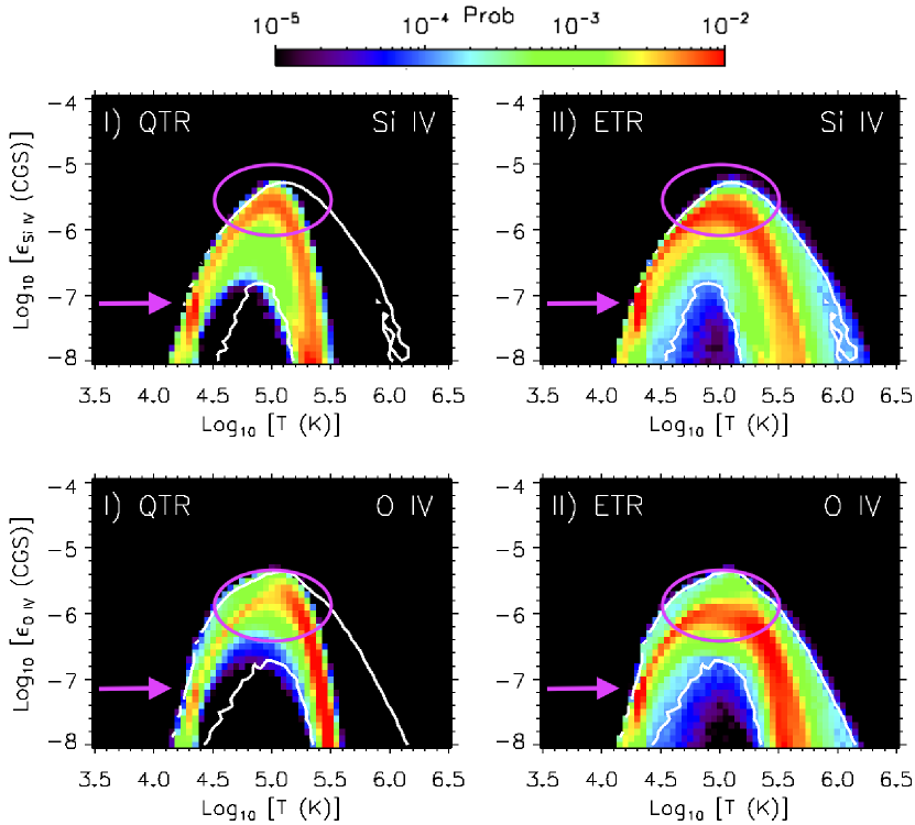
Figure 5: JPDFs of emissivity and temperature in the QTR and ETR in the vertical experiment for Si IV (top row) and O IV (bottom row) for the time range $t=55.0$ minute to $t=70.7$ minute. The size of the sample is $4\times 10^{6}$ elements. The white lines are isocontours of probability equal to $10^{-4}$ in the ETR distribution. The areas marked by ovals and arrows are discussed in the text.

We start analyzing the QTR and ETR distributions for the Si IV emissivity (see top row of Figure 5). The main result is that in the region with the largest emissivity values the ETR is more densely populated than the QTR (see the region marked by a pink oval around $\epsilon_{{}_{CGS}}\sim 10^{-5.6}$), i.e., the boundaries of the surges are more likely to show signal in Si IV observations than the QTR. This helps explain why, in the IRIS observations of our previous paper NS2017, we could detect the surge as an intrinsically brighter structure than the rest of the TR. Furthermore, both the QTR and ETR have the greatest values of emissivity in the temperature range between $10^{5.0}$ and $10^{5.1}$ K. This differs from what one would expect in SE, where the maximum emissivity is located at the peak formation temperature ($T_{{}_{SE}}=10^{4.9}$ K, see Table 1), again an indicator of the importance of taking into account NEQ effects. Additionally, the distribution both for QTR and ETR is more spread in temperature than what one would expect from a transition region distribution computed in SE (see, e.g., Figure 15 of the paper by Olluri et al., 2015). The mass density found both for QTR and ETR around the maximum Si IV emissivity is $\rho\sim 6.3\times 10^{-15}$ g cm^-3.

As part of the analysis, we have also found other features worth mentioning:

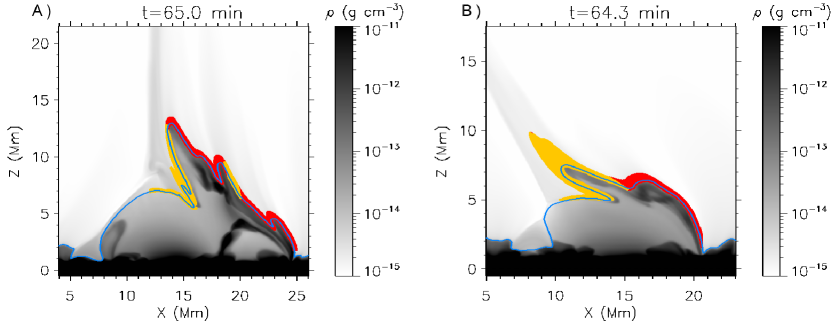
Figure 6: Density map showing the basic distribution of the (approximately) 6000 Lagrange tracers used in the text, distributed into two parts drawn with yellow and red dots corresponding to the two populations discussed in Section 4.3. The accompanying animation shows the evolution of the Lagrange tracers in the two experiments from early stages of the surge formation ($t\approx 55.0$ minute) until the its decay phase ($t\approx 70.0$ minute). (An animation of this figure is available.)

• The ETR has a broader temperature distribution than the QTR. In order to illustrate this fact, all the panels of Figure 5 contain isolines in white for the probability $10^{-4}$ in the ETR. The comparison of those contours with the QTR distribution shows that the ETR has a wider distribution in temperature, specially above $10^{5.5}$ K. Although not shown in the figure, the mass density values for most of the emitting plasma (more precisely: the mass density values with probability above $10^{-4}$) are constrained to similar ranges for both the QTR and ETR: approximately at [$2.0\times 10^{-15}$, $7.9\times 10^{-14}$] g cm^-3, for the vertical experiment; and at [$1.0\times 10^{-15}$, $6.0\times 10^{-14}$] g cm^-3, for the slanted one.

• A secondary probabilty maximum is located $\epsilon_{{}_{CGS}}\sim 10^{-7.2}$ and T $\sim 10^{4.3}$ K (see the arrows in the panels). This corresponds to the temperature of the second ionization of helium according to the LTE equation-of-state of Bifrost: the energy deposited in the plasma is used to ionize the element instead of heating the plasma. Including the NEQ ionization of helium should scatter the density probability in temperatures, as shown by Golding et al. (2016) in the TR of their numerical experiments (the equivalent to our QTR); nevertheless, the NEQ computation of helium and a detailed discussion of their effects are out of scope of this paper.

4.2.2 Plasma emitting in O IV

Focusing now on the statistical properties of the O IV emission (see bottom row of Figure 5), we see that, like for Si IV, the probability distributions for both QTR and ETR differ from what we could expect for a SE distribution, since they are centered at temperatures between $10^{4.9}$ and $10^{5.0}$ K instead of $T_{{}_{SE}}=10^{5.2}$ K (see Table 1). Furthermore, also here, the ETR and QTR distributions are broader in temperature than what one would expect from SE. Further noteworthy features of the plasma emitting in O IV are:

• The QTR exhibits larger probability than the ETR ($>10^{-3}$) in the maximum values of the emissivities ($\epsilon_{{}_{CGS}}=10^{-5.8}$); nevertheless, this fact changes around $\epsilon_{{}_{CGS}}=10^{-6.0}$, where the ETR shows larger emissivity (compare the region within the colored oval). Due to this complex behavior, we need to integrate the emissivity to know whether the ETR can be detected as a brighter structure compared to the QTR. In Section 5 we discuss this fact analyzing the obtained synthetic profiles.

• The ETR shows emissivity in O IV in a larger range of temperatures than the QTR, which is akin to the result for Si IV described in Section 4.2.1. This difference in the ranges is apparent mainly in hot coronal temperatures comparing the probability contours of the ETR (in white) with the QTR distribution.

• We find the same secondary probability maximum as in the Si IV panels at the temperature of the second ionization of helium (see the pinks arrows).

• Comparing the O IV panels with the Si IV ones, we see that the O IV distribution is more populated in hot temperatures, and correspondingly, lower densities. This is something we could expect since the ionization of this particular oxygen ion occurs at higher temperatures than Si IV.

4.3 Lagrange tracing: how the entropy sources affect the NEQ ionization

We focus now on the role of the entropy sources in the emissivity and NEQ ionization. To that end, we follow in time $\approx 6000$ plasma elements of the ETR through Lagrange tracing. In the following, we explain the set up for the Lagrange elements (Section 4.3.1) and the results obtained from their tracing (Section 4.3.2).

4.3.1 The choice of the Lagrange elements

The Lagrange elements are selected at a given instant, corresponding to an intermediate evolutionary stage when the surge is clearly distinguishable as a separate structure from the dome. The selected instants are $t=64.3$ minute for the slanted experiment and $t=65.0$ minute for the vertical experiment, which are the same times used for Figures 2, 3, and 4. In order to focus on the domain in and near the surge, we limit the selection to the rectangular areas: $12.0\leq x\leq 25.2$, $2.2\leq z\leq 15.0$ (vertical experiment); and $7.0\leq x\leq 19.0$, $5.0\leq z\leq 15.0$, and $19.0\leq x\leq 20.5$, $1.5\leq z\leq 15.0$ (slanted experiment). On those rectangles we lay a grid with uniform spacing $\Delta x=\Delta z=40$  km: the Lagrange elements are chosen among the pixels in that grid. A further criterion is then introduced: we are interested in studying the origin and evolution of the plasma elements with strong emission in Si IV and O IV. Thus, a lower bound in the Si IV and O IV emissivity is established, namely $\epsilon_{{}_{CGS}}>10^{-10}$, discarding all the pixels with emissivities below that value at the instants mentioned in the previous bullet point. The resulting choice of Lagrange tracers is shown in Figure 6 as red and yellow dots (the colors serve to distinguish the populations described below). Once the distribution is set, we then follow the tracers backward in time for 10 minutes, to study their origin, and forward in time for 5.7 minutes, to see the whole surge evolution until the decay phase, with a high temporal cadence of $0.2$ seconds (see the accompanying animation to Figure 6).

4.3.2 Plasma populations and role of the entropy sources

Studying the time evolution of the Lagrange tracers, in particular their thermal properties, one can distinguish two populations that are the source of the Si IV and O IV emission: one originating in the emerged dome (yellow plasma population in Figure 6) and the other one originating in the corona (red population). By carefully inspecting the tracers of each population, we find that their behavior is well defined: the major difference between the elements within the same population is not the nature or order of the physical events described below, but rather the starting time of the evolution for each tracer. Figure 7 contains the time evolution of different quantities as measured following a representative Lagrange element of each population, namely temperature, $T$, (green); Si IV emissivity, $\epsilon_{{}_{Si\ IV}}$, (dark blue); O IV emissivity, $\epsilon_{{}_{O\ IV}}$, (light blue); characteristic time of the optically thin losses, $\tau_{thin}$, (black); and characteristic time for the thermal conduction, $\tau_{Spitz}$ (red).

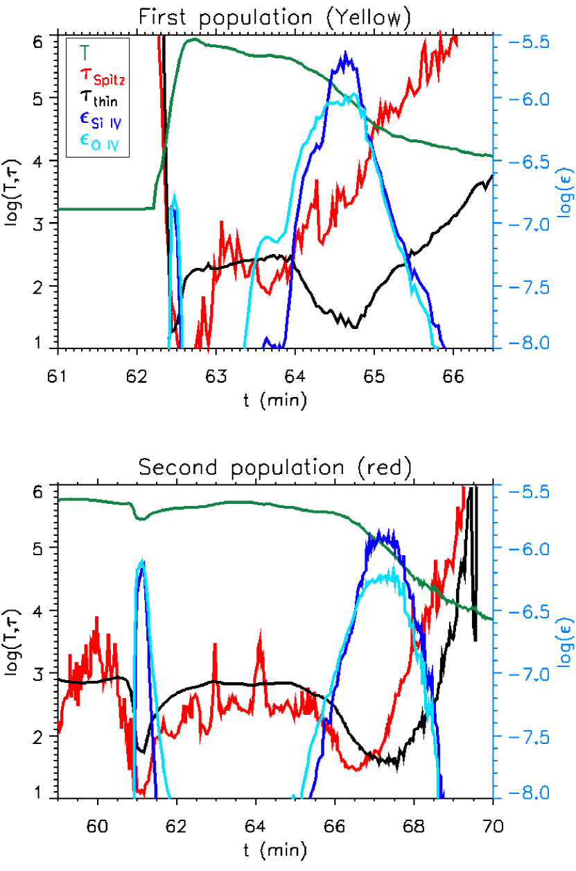
Figure 7: Time evolution of key physical quantities for representative Lagrange tracers in the vertical experiment of Figure 5. Top: Lagrange element coming from the emerged dome (yellow population in Figure 6). Bottom: Lagrange originating in the corona (red population in Figure 6). The curves show (left ordinate axis) the logarithm of temperature $T$ (green); of the characteristic time of the optically thin losses $\tau_{thin}$ (black); and of the characteristic time for the thermal conduction $\tau_{Spitz}$ (red); and (right ordinate axis) the logarithm of the Si IV emissivity (dark blue); and of the O IV emissivity (light blue). All quantities are in CGS units.

The first population (top panel of Figure 7, corresponding to the elements marked in yellow in Figure 6), starts as cool and dense plasma coming from the emerged dome with extremely low emissivity (see the curves for the temperature in green, and for the emissivities in dark and light blue). At some point that plasma approaches the reconnection site and passes through the current sheet, thereby suffering strong Joule and viscous heating and quickly reaching TR temperatures. The sharp spike in the Si IV and O IV emissivity (blue curves) around $t\sim 62.5$ minute corresponds to this phase: the temperature increase leads to the appearance of those ionic species, but, as the plasma continues being heated, it reaches high temperatures (maximum around $10^{6}$ K) and the number densities $n_{u}$ of Si IV and O IV decrease again. At those high temperatures the entropy sinks become efficient, with short characteristic times: see the red ($\tau_{Spitz}$) and black ($\tau_{thin}$) curves. The plasma thus enters a phase of gradual cooling, going again through TR temperatures, renewed formation of the Si IV and O IV ions, and increase in the corresponding emissivity (broad maximum in the blue curves in the right half of the panel). The plasma elements, finally, cool down to chromospheric temperatures, with the emissivity decreasing again to very low values.

The defining feature of the second population (bottom panel of Figure 7, red dots in Figure 6) is that it originates in the corona as apparent in the temperature curve (green). This population starts at heights far above the reconnection site, with standard coronal temperature and density. During the magnetic reconnection process, its associated field line changes connectivity, becoming attached to the cool emerged region. Consequently, a steep temperature gradient arises along the field line, so the thermal conduction starts to cool down the plasma; given the temperature range, also the optically thin losses contribute to the cooling, although to a lesser extent (see the $\tau_{Spitz}$ and $\tau_{thin}$ curves around $t\sim 61$ minute, in red and black, respectively). The temperature drops to values around T $\sim 10^{5.5}$ K, which, according to the JPDFs of Figure 5, makes it sufficiently likely that the Si IV and O IV emissivities from the Lagrange element are high. This explains the large increase, by a few orders of magnitude, in the blue emissivity curves around $t\sim 61$ minute (although a small factor $\sim 4$ is due to the simultaneous increase in the mass density, which is reflected in a linear fashion in the emissivity). This cooling to TR temperatures, however, is short lived: as the plasma element itself passes near the current sheet, it can be heated because of the Joule and viscous terms and the temperature climbs again to values where the emissivities are low: hence the sharp spike in the blue curves between $t\sim 61$ and $t\sim 61.5$ minute. There ensues a phase of gradual cooling from $t\sim 64$ onward, similar to what happened to the previous population, with characteristic cooling times of a few to several hundred seconds (see red and black curves), passage through TR temperatures, broad maximum in the emissivity curves and with the plasma finally reaching chromospheric temperatures.

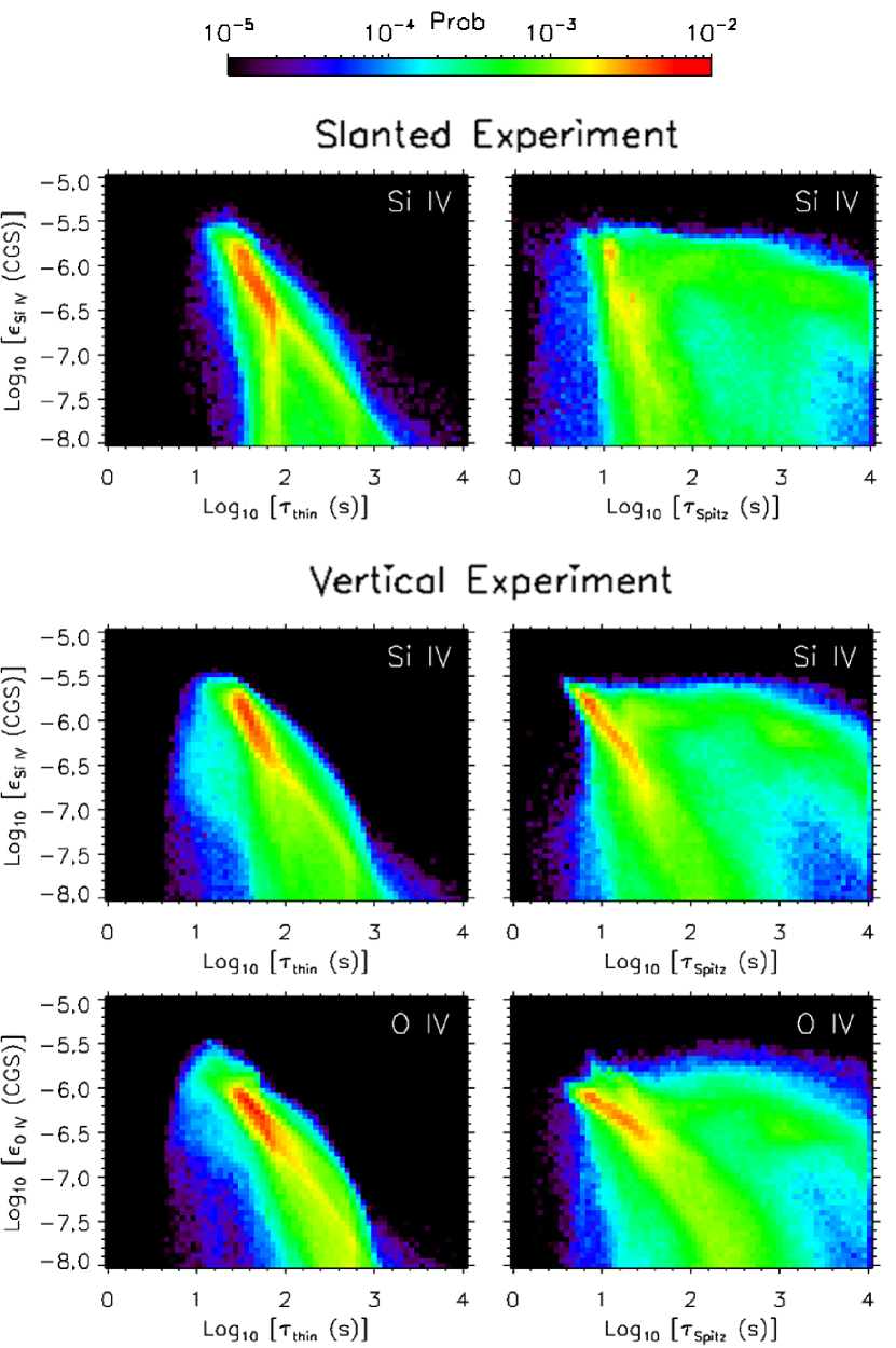
Figure 8: JPDFs for the Si IV and O IV emissivity of the Lagrange tracers over $15.7$ minutes versus the characteristic time of the optically thin losses ($\tau_{thin}$, left column) and the thermal conduction ($\tau_{Spitz}$, right column).

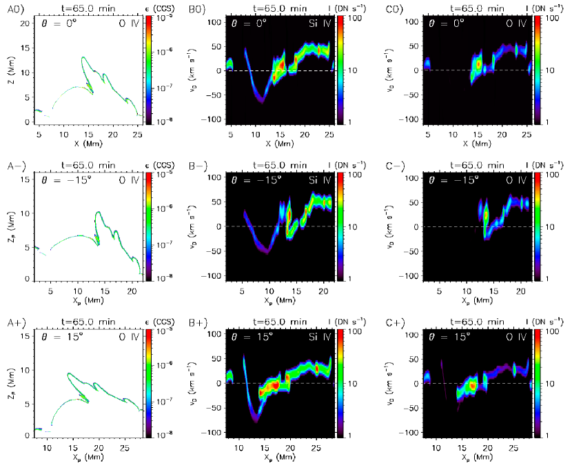
Figure 9: Synthetic profiles for the vertical experiment at different times for various LOS ($\theta$). A) 2D map of the $\epsilon_{{}_{CGS}}$ for O IV to show the context; B) synthetic spectral intensity for Si IV, and ; C) synthetic spectral intensity for O IV. To identify the LOS of each panel, we have added the symbols $0$, $-$, and $+$ respectively to $\theta=0,-15$ and $15$ °. In the $\theta\neq 0$ rows, $z_{P}$ and $x_{P}$ are, respectively, the vertical and horizontal coordinates of the rotated figures. The animation of this figure shows the time evolution of the surge from its origin ($t=61$ minute) up to its decay phase ($t=70.7$ minute) in the vertical experiment for the three LOS. (An animation of this figure is available.)

In our previous paper (NS2016) we found that surges were constituted by four different populations according to their thermal evolution. In the current paper, we see that only two of them, labelled Populations B and D in the NS2016 paper, are behind the enhanced emissivity of TR lines like those from silicon and oxygen discussed here. The other two populations described by NS2016 (A and C) keep cool chromospheric temperatures during their evolution and do not play any role for the TR elements.

Using the Lagrange tracing method developed here, we can produce conclusive evidence of enhanced Si IV and O IV emissivity and occurrence of fast evolution due to short-time scales in the entropy sources associated with heat conduction or optically thin radiative cooling. Figure 8 contains double PDFs for $\epsilon{{}_{CGS}}$ versus $\tau_{thin}$ (left panels) and $\tau_{Spitz}$ (right panels) using as statistical sample the values of those quantities for all Lagrange tracers along their evolution. The choice of the ionic species (Si IV, O IV) and experiment (slanted, vertical) in the panels is as in Figures 3 and 4. The figure clearly shows that when the entropy sources act on short time scales, the (Si IV, O IV) emissivities are large. In fact, the maximum values of $\epsilon{{}_{CGS}}$ correspond to characteristic cooling times between $20-100$ s for $\tau_{thin}$ and between $4-40$ s for $\tau_{Spitz}$. Those changes are fast enough for the ionization levels of those elements to be far from statistical equilibrium.

5 Observational consequences

In the paper by NS2017, different observed Si IV signatures within the surge were analyzed. Moreover, counterparts to the observational features were identified in the synthetic spectral profiles obtained from the numerical model; however, a theoretical analysis to understand the origin of the spectral features and the reason for the brightness in the various regions of the surge was not addressed. In the following subsection a theoretical study is carried out trying to quantify the impact of the NEQ ionization of silicon and oxygen on the spectral and total intensities and the observational consequences thereof (Section 5.1). Then, given the involved geometry of the surge, the particular LOS for the (real or synthetic) observation turns out to be crucial for the resulting total intensity and spectra. This is studied in Section 5.2.

5.1 Synthetic profiles

Figure 9 contains the synthetic profiles obtained by integrating the emissivity along the line of sight for different wavelengths in the Si IV $1402.77$ Å and O IV $1401.16$ Å spectral region and for the vertical experiment. The three rows of the figure correspond to different inclination angles $\theta$ for the LOS: from top to bottom, 0°, -15° and 15°, respectively. The panels in each row contain A) the context of the experiment through a 2D map of the O IV emissivity; B) the synthetic spectral intensity for Si IV with the spectral dimension in ordinates and in the form of Doppler shifts from the central wavelength; and C) the corresponding synthetic spectral intensity for O IV. Those spectra are obtained taking into account the Doppler shift due to the plasma velocity and applying a spatial and spectral PSF (Gaussian) degradation as explained in detail by Martínez-Sykora et al. (2016), their section 3.1, and by NS2017, their section 2.2. In this way, we will be able to directly compare the results with IRIS observations. In order to ease the identification of the LOS in each panel, we have added to the labels on it, the symbols $0$, $-$, and $+$ respectively to $\theta=0,-15$ and $15$ °. In the middle and bottom rows of the image, $x_{P}$ and $z_{P}$ are, respectively, the horizontal and vertical coordinates of the rotated figures.

To extend the analysis, it is also of interest to consider the total emitted intensity for each vertical column, i.e.,

$$I_{\epsilon}(x) = \int_{z_{0}}^{z_{f}}{\epsilon\;dz}\;,$$ (5)

which, following Equation 1, is equal to the column density of the emitting species along the LOS except for a constant factor). Equation (5) has been calculated separately for Si IV and O IV and with the emissivities obtained assuming either NEQ or SE ionization, to better gauge the importance of disregarding the NEQ effects. The results are shown in the middle and bottom panel of Figure 10 for Si IV and O IV , respectively. The top panel of the image contains the 2D map of the emissivity for Si IV for context identification. Combining Figures 9 and 10, we are able to discern and describe characteristic features of the spectral profiles.

• The most prominent feature in the synthetic profiles of Figure 9 is the brightening associated with the location of the internal footpoint of the surge. In the corresponding movie, we can see how that footpoint is formed at around $t=64$ minute, as the surge detaches from the emerged dome. During those instants, the associated synthetic profiles are characterized by large intermittent intensities and bidirectional behavior with velocities of tens of km s^-1, as apparent, e.g., in the B0 and C0 panels at $x\in[15,16]$ Mm. In Si IV and O IV (B and C panels), we find that the internal footpoint is usually the brightest region, although there are some instants in which the brightest points can be located in the crests or the external footpoint. This is a potentially important result from the observational point of view because it can help us to unravel the spatial geometry of the surge in future observational studies: if strong brightenings are detected in Si IV and also in O IV within the surge, it would be reasonable to think that they correspond to the internal footpoint of the surge. In this region, the intensity ratio between Si IV and O IV ranges between 2 and 7, approximately. Note that, in general, the intensity ratio values vary depending on the observed region and features (Martínez-Sykora et al., 2016).

  In Section 5.2 we will see that LOS effects play a major role in causing the large brightness of the internal footpoint (and other bright features) compared to the rest of the surge. Here we consider the parallel question of the role of NEQ: what would be obtained for the intensity of the internal footpoint if SE were assumed? Comparing the values for Si IV in Figure 10 (middle panel, $13.8\leq x\leq 16.1$), there is roughly a factor $2$, in the average, between the NEQ and SE intensities; for O IV (bottom panel), there is no major difference in the intensity between both calculations. One could conclude that while NEQ is important for the Si IV diagnostics, SE could be applied for the O IV case; nonetheless, even in the latter case, although the NEQ and SE intensities are similar, one would make a mistake in the determination of derived quantities like the number densities of emitters (Section 4.1) and temperatures (Section 4.2).

  Further distinctive brightenings in the spectral profiles appear at the site of the crests and of the external footpoint of the surge. The brightness of those regions is clear in the Si IV profiles (B0, B$-$ and B$+$ panels of Figure 9) through their large intensity, and is sometimes comparable or greater than that of the internal footpoint (see, e.g., the locations at $x\sim 13$, $18$, $23$ and $25$ Mm in the top row, or, $x\sim 14,19$ and $25$ Mm in the bottom row). In the O IV profiles (C0, C$-$ and C$+$ panels), although faint in comparison with Si IV (around a factor 5 less intense), most of those features are still slightly brighter than the rest of the surge. This difference in intensities between Si IV and O IV can also be used to understand the observations: if strong signals are observed in Si IV associated with some moderate signal in O IV, it could indicate that we are detecting the crests or the external footpoint. Concerning the NEQ/SE comparison of the intensity (Figure 10), the crests and footpoints show the same behavior as the internal footpoint.

• The intensity of the rest of the surge is small in comparison with that of the footpoints and crests just described, so we wonder whether one could see it as a bright structure in actual observations and distinguish it from the rest of the TR. In the middle panel of Figure 10, comparing the $I_{\epsilon}$ values for Si IV within the ETR against those in the QTR, we can see that all the regions in the surge have a higher intensity than the QTR; outside of the brightest features, the excess emission of Si IV in the surge may be just a factor 2 or 3 above the QTR, but that can provide enough contrast to tell the two regions apart observationally, as found in the NS2017 paper. Note, importantly, that there is a large difference between the NEQ and SE results for Si IV in the surge, up to a factor 10, so the SE assumption would seriously underestimate the intensity. In fact, in most of the places Si IV would be similar or fainter than O IV if SE were valid as shown also, e.g. by Dudík et al. (2014) and Dzifčáková et al. (2017). On the other hand, for O IV (bottom panel), the prominent features are the footpoints and crests of the surge, while the other parts have $I_{\epsilon}$ comparable to the QTR. As a consequence and from an observational point of view, while in Si IV we could find enhanced emission in the whole surge (which is compatible with the NS2017 observation), for O IV only the brightest regions would stand out, namely, the internal footpoints and, to a lesser extent, the crests and external footpoints.

  The underlying reason for the enhanced brightness of all those features, mainly the footpoints and crests of the surges, is not just the presence of additional numbers of ions due to NEQ effects: the complex geometry of the surge TR has important consequences when integrating the emissivity along the line of sight to obtain intensities . This is discussed in the next section.

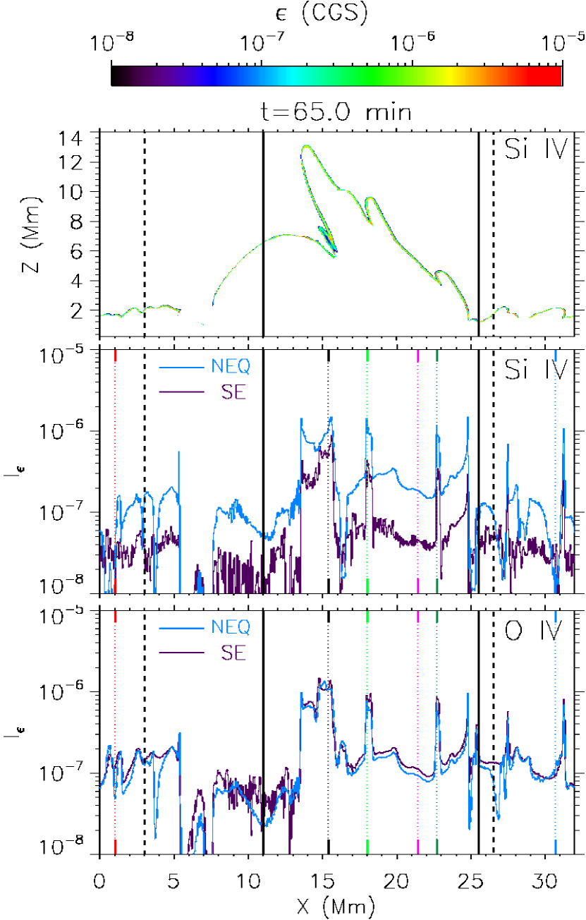
Figure 10: Top panel: 2D map of the Si IV emissivity. The vertically integrated intensity $I_{\epsilon}$ is shown both for Si IV (middle panel) and O IV (bottom panel) assuming NEQ ionization (light blue curve) and SE (purple). Solid and dashed lines are overplotted in the image to delimit the ETR and QTR regions as in previous figures. Dotted vertical lines are superimposed in the middle and bottom panel correspondingly to the cuts shown in Figure 11.

5.2 The role of the LOS

The observation of TR lines generated in the surge strongly depends on the particular LOS. We show this here through two different effects:

1. The alignment of the LOS with respect to the orientation of the surge’s TR. We can appreciate this effect, e.g., in A0 panel of Figure 9. There, considering, e.g., the crests situated at $x=13.5$, $x=18$ or $x=23$ Mm, we see that a vertical LOS grazing the left side of the crest will include contributions from a much larger length of the TR than if the crossing were perpendicular or nearly so. The same can be said of the external footpoint at $x=24.8$ Mm and also of the internal footpoint around $x=16$ Mm. This effect clearly enhances the brightenings seen in those values of $x$ in panels B0 and C0. Further evidence can be found by checking the $I_{\epsilon}$ curves in the middle and bottom panels of Figure 10; in fact, since the effect is purely geometrical, the contribution to brightness can be seen both in the NEQ and SE curves in the two panels of the figure. Varying the angle of the LOS, we can reach enhancement factors between 2 and 4; nonetheless, discerning which part of that factor is exclusively due to the LOS is complicated, since variations in the angle of integration imply integrations along slightly different emitting layers. Additionally, the inclination of the LOS with respect to the surge’s TR may be important for the apparent horizontal size of the brightenings. This can be seen through comparison of the three rows of Figure 9: considering the size of the brightening associated with the internal footpoint, we see that it covers a larger horizontal range in the $\theta=0$° and $\theta=15$° cases (top and bottom rows), than in the $\theta=-15$° case (middle row), since the good alignment of the latter is lost in the former.

2. The multiple crossings of the TR by individual lines of sight. Given that the TR of the surge is folded, there are horizontal ranges in which the LOS crosses it more than once (typically three times, in some limited ranges even five times). Given the optically thin approximation, the emitted intensity in those lines of sight may be a few, or several, times larger than the value in a single crossing.

To further illustrate those two effects, we use Figure 11. The top panel contains a 2D map of the Si IV emissivity in which vertical cuts in different regions of interest are overplotted through colored and labelled lines. The corresponding Si IV emissivity distribution along those cuts is shown in panel B. Additionally, a similar plot but for the O IV distribution is shown in panel C. Those vertical cuts are also shown in panels B and C of Figure 10 for comparison purposes. The light and dark green cuts (numbers 3 and 5) are typical examples of the effect of the tangency between the LOS and the surge’s TR at the crests: note the enhanced width of the maximum on the right in those two cuts due to tangency effects. Those cuts and the one in black (number 2) further show the effect of multiple crossings of the TR by the LOS. In particular, the LOS drawn in black crosses the folded TR near the internal footpoint four times ($5.5<z<8$ Mm), and an additional time at the the top of the surge ($z\sim 11$ Mm). For the sake of completeness, we have added a dashed line for the crests (3 and 5) in the middle and lower panels showing the emissivity if SE had been assumed: the thickness of the high-emissivity TR would be much smaller. Finally, in contrast to all the foregoing cases, the rest of the surge (pink line, label 4) and the QTR (red and blue lines, labels 1 and 6, respectively) show a simpler geometry, there is no TR-LOS alignment and there is just a single crossing.

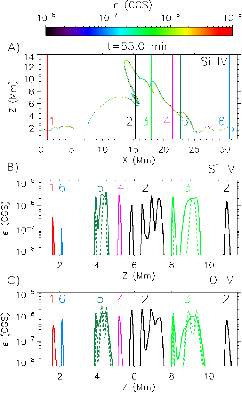
Figure 11: Illustration of the multiple crossings of the transition region by a single LOS. A) 2D map of the Si IV emissivity with colored and labelled lines overplotted in regions of interest. The lines corresponds to different vertical cuts used in panels B and C. B) Si IV emissivity versus the height $Z$ for the different vertical cuts shown in the 2D map. C) Like panel B but for the O IV emissivity. Additionally, for the cuts labelled 3 and 5 we have added as a dashed line the corresponding emissivity if SE had been assumed.

6 Discussion

In this paper, we have carried out two 2.5D radiative-MHD numerical experiments of magnetic flux emergence through granular convection and into the solar atmosphere. The experiments were performed with Bifrost, including an extra module of the code that computes the nonequilibrium ionization (NEQ) of silicon and oxygen. The time evolution of the two experiments leads to the formation of a cool and dense surge. We have studied the relevance of the NEQ ionization for the presence of Si IV and O IV in the periphery of the surge and how it affects the corresponding emissivities. The properties of the surge plasma emitting in Si IV and O IV were then characterized and compared with those of the general TR plasma outside of the surge. We have also analyzed the role of the heat conduction and optically-thin radiative cooling in the NEQ ionization. Furthermore, through forward modelling, we have understood different features of the synthetic spectral profiles of Si IV and O IV, explaining the importance of the shape of the transition region surrounding the surge combined with the different possible angles of the LOS and providing predictions for future observational studies.

In the following, we first address the implications of the importance of the NEQ ionization in numerical experiments of eruptive phenomena in which heating and cooling are key mechanisms. (Section 6.1). We then discuss their relevance for present and future observations (Section 6.2).

6.1 On the importance of the nonequilibrium (NEQ) ionization

The main result of this paper is that the envelope of the emerged domain, more specifically, of the dome and surge, are strongly affected by NEQ ionization (Section 4.1). Focusing on the boundaries of the surge, comparing the number densities of emitters computed via detailed solution of the NEQ rate equations with those obtained assuming statistical equilibrium (SE) we have concluded that the SE assumption would produce an erroneous result in the population of Si IV and O IV, mainly because it leads to a gross underestimate of the number density of emitters. The transition region outside of the flux emergence site is also affected by NEQ, but to a smaller extent.

The above result has consequences in the corresponding emissivity (Section 4.2) and therefore, in the interpretation of the observations. By means of statistical analysis, we have shown that the boundaries of the surge have greater values of the Si IV emissivity than the region outside of the flux emergence site. Correspondingly, we have given the name enhanced transition region (ETR) to the former and quiet transition region (QTR) to the latter (Section 4.2.1). This difference is part of the explanation of why the surge is a brighter structure than the rest of the transition region in the IRIS observations by NS2017. Furthermore, the joint probability distributions for emissivity and temperature are not centered at the peak formation temperature of Si IV or O IV in SE (see $T_{{}_{SE}}$ in Table 1 and Section 4.2.2). This reinforces earlier results (e.g., Olluri et al., 2015) about the inaccuracies inherent in the process of deducing temperature values from observations in transition region lines using SE considerations.

In Section 4.3 we have found that there are two different populations concerning the thermal evolution that leads to the Si IV and O IV emissivity. They have very different origins (one in the emerged plasma dome, the other in coronal heights) but both are characterized by the fact that they go through a period of rapid thermal change caused by the optically thin losses and thermal conduction: the maximum values of the Si IV and O IV emissivity in them are related to short characteristic cooling times: $20-100$ s for $\tau_{thin}$ and around $4-40$ s for $\tau_{Spitz}$. Those characteristic times are compatible with the theoretical results by Smith & Hughes (2010), who found that for typical densities of the active corona and the transition region, the solar plasma can be affected by NEQ effects if changes occur on timescales shorter than about $10-100$ s. Those results highlight the role of optically thin losses and thermal conduction because a) they provide the physical mechanism to diminish the entropy and, consequently, obtain plasma with the adequate temperatures to form ions of Si IV or O IV ($\sim 10^{5}$ K ); and b) they are fast enough to produce important departures from SE. On the other hand, the ion populations calculated through the present NEQ module in Bifrost are not used in the energy equation of the general R-MHD calculation (see Section 2.1), so this could underestimate the effects of the entropy sinks in the experiments. In fact, Hansteen (1993) found deviations of more than a factor two in the optically thin losses when considering nonequilibrium effects in his loop model, so $\tau_{thin}$ could be even more efficient.

Our results indicate that surges, although traditionally described as chromospheric phenomena, show important emission in transition region lines due to the NEQ ionization linked to the quick action of the cooling processes, so the response of the transition region is intimately tied to the surge dynamics and energetics. In fact, the same statement may apply for other eruptive phenomena, in which impulsive plasma heating and cooling occurs (see Dudík et al., 2017, for a review of NEQ processes in the solar atmosphere).

6.2 Understanding observations and predictions for the future

From the number density of emitters and emissivity results of Section 4 we gather that calculating heavy element populations directly through the rate equations instead of via the assumption of statistical equilibrium can be important to understand the observations of surges (and of other fast phenomena which reach TR temperatures in their periphery like spicules De Pontieu et al. 2017, or UV bursts Hansteen et al. 2017). In that section, analyzing the Si IV and O IV emissivities of the plasma elements, we find that the ratio between them is approximately 2 in the regions with the highest emission within the ETR. Even though the intensity ratio is more commonly used (Hayes & Shine, 1987; Feldman et al., 2008; Polito et al., 2016, among others), the emissivity ratio can also be a valuable tool to understand the behavior of the ions in different regions of the Sun. In particular, we see that in the ETR this ratio is larger than in the transition region that has not been perturbed by the flux emergence and subsequent surge and/or jet phenomena (QTR).

To provide theoretical support to the NS2017 observations and predictions for future ones, in Section 5 we have therefore computed the synthetic profiles of Si IV 1402.77 Å and O IV 1401.16 Å, taking into account the Doppler shift because of the plasma velocity and degrading the spatial and spectral resolutions to the IRIS ones. A line-of-sight integration of the emissivities has also been carried out, to provide a measure for the total intensity emitted by the different regions of the surge. The strongest brightenings in Si IV and O IV have been located at the site of the internal footpoint, followed by the crests and the external footpoint (Figure 9, Section 5.1). The intensity ratio between Si IV and O IV in those regions is, approximately, 5 (although it can range from 2 and 7). Those values are between those for a coronal hole and a quiescent active region obtained by Martínez-Sykora et al. (2016), which is consistent since we are mimicking an initial stratification similar to a coronal hole in which a total axial magnetic flux in the range of an ephemeral active region (Zwaan, 1987) has been injected. The comparison of the total intensity for the NEQ and SE cases (Figure 10, Section 5.1) leads to a further indication of the importance of using NEQ equations to determine the number density of Si IV: the NEQ calculation yields intensities coming out of the surge which are a factor between $2$ and $10$ larger than when SE is assumed. For O IV, instead, the NEQ and SE calculations yield similar integrated intensities. For O IV, therefore, the NEQ calculations are important mainly to determine derived quantities like number densities of emitters $n_{u}$ (Section 4.1) and temperatures (Section 4.2). In addition, we have found that for Si IV all the regions in the surge have a greater intensity than the QTR: this can explain why the surge can be observationally distinguished from the QTR, as found in the NS2017 paper.

The high brightness of various features in the surge has been seen to arise in no small part from different LOS effects tied to the peculiarly irregular shape of its TR, and, in particular, to its varying inclination and the folds that develop in it (Section 5.2). On the one hand, whenever LOS and tangent plane to the TR are not mutually orthogonal, the issuing intensity collects emissivity from a larger number of plasma elements in the TR (alignment effect); on the other hand, given that the surge’s TR is variously folded, forming crests and wedges, the LOS crosses the emitting layer multiple times (multiple-crossing effect). The alignment and multiple-crossing effects are quite evident in the footpoints and crests. This explains their remarkable brightness and makes clear their potential as beacons to indicate the presence of those special features in surge-like phenomena when observed in TR lines like Si IV (Figure 11). Additionally, the multiple crossings can also have an impact on the observed Doppler shifts since we could be integrating various emitting layers with different dynamics. So, when confronted with a TR observation of a region where a surge is taking place, the detection of strong brightenings in Si IV and O IV could help unravel the geometry of the surge. Furthermore, since the internal footpoint of the surge is close to the reconnection site, we might also find observational evidences of reconnection in the neighborhood. This provides theoretical support to the location of the brightenings in the IRIS observations by NS2017. In addition, if strong signals are observed in Si IV related to some moderate signal in O IV, they could correspond to the crests and the external footpoint of the surge; nonetheless, the rest of the surge structure could be only differentiated from the transition region in Si IV.

References

- Asplund et al. (2009) Asplund, M., Grevesse, N., Sauval, A. J., & Scott, P. 2009, ARA&A, 47, 481
- Bohlin et al. (1975) Bohlin, J. D., Vogel, S. N., Purcell, J. D., Sheeley, Jr., N. R., Tousey, R., & Vanhoosier, M. E. 1975, ApJ, 197, L133
- Bradshaw & Cargill (2006) Bradshaw, S. J., & Cargill, P. J. 2006, A&A, 458, 987
- Bradshaw & Klimchuk (2011) Bradshaw, S. J., & Klimchuk, J. A. 2011, ApJS, 194, 26
- Bradshaw & Mason (2003) Bradshaw, S. J., & Mason, H. E. 2003, A&A, 401, 699
- Canfield et al. (1996) Canfield, R. C., Reardon, K. P., Leka, K. D., Shibata, K., Yokoyama, T., & Shimojo, M. 1996, ApJ, 464, 1016
- Carlsson & Leenaarts (2012) Carlsson, M., & Leenaarts, J. 2012, A&A, 539, A39
- Chae et al. (1998) Chae, J., Schühle, U., & Lemaire, P. 1998, ApJ, 505, 957
- De Pontieu et al. (2017) De Pontieu, B., De Moortel, I., Martinez-Sykora, J., & McIntosh, S. W. 2017, ApJ, 845, L18
- De Pontieu et al. (2015) De Pontieu, B., McIntosh, S., Martinez-Sykora, J., Peter, H., & Pereira, T. M. D. 2015, ApJ, 799, L12
- De Pontieu et al. (2007) De Pontieu, B., et al. 2007, PASJ, 59, 655
- De Pontieu et al. (2014) —. 2014, Sol. Phys.
- Doschek (2006) Doschek, G. A. 2006, ApJ, 649, 515
- Doschek et al. (2008) Doschek, G. A., Warren, H. P., Mariska, J. T., Muglach, K., Culhane, J. L., Hara, H., & Watanabe, T. 2008, ApJ, 686, 1362
- Drews & Rouppe van der Voort (2017) Drews, A., & Rouppe van der Voort, L. 2017, A&A, 602, A80
- Dudík et al. (2014) Dudík, J., Del Zanna, G., Dzifčáková, E., Mason, H. E., & Golub, L. 2014, ApJ, 780, L12
- Dudík et al. (2017) Dudík, J., et al. 2017, Sol. Phys., 292, 100
- Dzifčáková et al. (2017) Dzifčáková, E., Vocks, C., & Dudík, J. 2017, A&A, 603, A14
- Feldman et al. (2008) Feldman, U., Landi, E., & Doschek, G. A. 2008, ApJ, 679, 843
- Georgakilas et al. (1999) Georgakilas, A. A., Koutchmy, S., & Alissandrakis, C. E. 1999, A&A, 341, 610
- Golding et al. (2014) Golding, T. P., Carlsson, M., & Leenaarts, J. 2014, ApJ, 784, 30
- Golding et al. (2016) Golding, T. P., Leenaarts, J., & Carlsson, M. 2016, ApJ, 817, 125
- Griem (1964) Griem, H. R. 1964, Plasma spectroscopy
- Gudiksen et al. (2011) Gudiksen, B. V., Carlsson, M., Hansteen, V. H., Hayek, W., Leenaarts, J., & Martínez-Sykora, J. 2011, A&A, 531, A154+
- Guglielmino et al. (2010) Guglielmino, S. L., Bellot Rubio, L. R., Zuccarello, F., Aulanier, G., Vargas Domínguez, S., & Kamio, S. 2010, ApJ, 724, 1083
- Hansteen (1993) Hansteen, V. 1993, ApJ, 402, 741
- Hansteen et al. (2017) Hansteen, V. H., Archontis, V., Pereira, T. M. D., Carlsson, M., Rouppe van der Voort, L., & Leenaarts, J. 2017, ApJ, 839, 22
- Hansteen et al. (2006) Hansteen, V. H., De Pontieu, B., Rouppe van der Voort, L., van Noort, M., & Carlsson, M. 2006, Apj, 647, L73
- Hayek et al. (2010) Hayek, W., Asplund, M., Carlsson, M., Trampedach, R., Collet, R., Gudiksen, B. V., Hansteen, V. H., & Leenaarts, J. 2010, A&A, 517, A49+
- Hayes & Shine (1987) Hayes, M., & Shine, R. A. 1987, ApJ, 312, 943
- Jiang et al. (2012) Jiang, R.-L., Fang, C., & Chen, P.-F. 2012, ApJ, 751, 152
- Joselyn et al. (1979) Joselyn, J. A., Munro, R. H., & Holzer, T. E. 1979, ApJS, 40, 793
- Katsukawa et al. (2007) Katsukawa, Y., et al. 2007, Science, 318, 1594
- Kayshap et al. (2013) Kayshap, P., Srivastava, A. K., Murawski, K., & Tripathi, D. 2013, ApJ, 770, L3
- Kurokawa et al. (2007) Kurokawa, H., Liu, Y., Sano, S., & Ishii, T. T. 2007, in Astronomical Society of the Pacific Conference Series, Vol. 369, New Solar Physics with Solar-B Mission, ed. K. Shibata, S. Nagata, & T. Sakurai, 347
- Leenaarts et al. (2011) Leenaarts, J., Carlsson, M., Hansteen, V., & Gudiksen, B. V. 2011, A&A, 530, A124
- Leenaarts et al. (2007) Leenaarts, J., Carlsson, M., Hansteen, V., & Rutten, R. J. 2007, A&A, 473, 625
- MacTaggart et al. (2015) MacTaggart, D., Guglielmino, S. L., Haynes, A. L., Simitev, R., & Zuccarello, F. 2015, A&A, 576, A4
- Martínez-Sykora et al. (2016) Martínez-Sykora, J., De Pontieu, B., Hansteen, V. H., & Gudiksen, B. 2016, ApJ, 817, 46
- Martínez-Sykora et al. (2008) Martínez-Sykora, J., Hansteen, V., & Carlsson, M. 2008, ApJ, 679, 871
- Moreno-Insertis & Galsgaard (2013) Moreno-Insertis, F., & Galsgaard, K. 2013, ApJ, 771, 20
- Murawski et al. (2011) Murawski, K., Srivastava, A. K., & Zaqarashvili, T. V. 2011, A&A, 535, A58
- Nishizuka et al. (2008) Nishizuka, N., Shimizu, M., Nakamura, T., Otsuji, K., Okamoto, T. J., Katsukawa, Y., & Shibata, K. 2008, ApJ, 683, L83
- Nóbrega-Siverio et al. (2017) Nóbrega-Siverio, D., Martínez-Sykora, J., Moreno-Insertis, F., & Rouppe van der Voort, L. 2017, ApJ, 850, 153
- Nóbrega-Siverio et al. (2016) Nóbrega-Siverio, D., Moreno-Insertis, F., & Martínez-Sykora, J. 2016, ApJ, 822, 18
- Olluri et al. (2013a) Olluri, K., Gudiksen, B. V., & Hansteen, V. H. 2013a, ApJ, 767, 43
- Olluri et al. (2013b) —. 2013b, AJ, 145, 72
- Olluri et al. (2015) Olluri, K., Gudiksen, B. V., Hansteen, V. H., & De Pontieu, B. 2015, ApJ, 802, 5
- Pereira et al. (2012) Pereira, T. M. D., De Pontieu, B., & Carlsson, M. 2012, ApJ, 759, 18
- Polito et al. (2016) Polito, V., Del Zanna, G., Dudík, J., Mason, H. E., Giunta, A., & Reeves, K. K. 2016, A&A, 594, A64
- Raymond & Dupree (1978) Raymond, J. C., & Dupree, A. K. 1978, ApJ, 222, 379
- Reep et al. (2016) Reep, J. W., Warren, H. P., Crump, N. A., & Simões, P. J. A. 2016, ApJ, 827, 145
- Rouppe van der Voort et al. (2017) Rouppe van der Voort, L., et al. 2017, ApJ, 851, L6
- Scharmer et al. (2003) Scharmer, G. B., Bjelksjo, K., Korhonen, T. K., Lindberg, B., & Petterson, B. 2003, in Society of Photo-Optical Instrumentation Engineers (SPIE) Conference Series, Vol. 4853, Society of Photo-Optical Instrumentation Engineers (SPIE) Conference Series, ed. S. L. Keil & S. V. Avakyan, 341–350
- Shibata et al. (1992) Shibata, K., Nozawa, S., & Matsumoto, R. 1992, PASJ, 44, 265
- Smith & Hughes (2010) Smith, R. K., & Hughes, J. P. 2010, ApJ, 718, 583
- Yang et al. (2014) Yang, H., Chae, J., Lim, E.-K., Lee, K.-s., Park, H., Song, D.-u., & Cho, K. 2014, ApJ, 790, L4
- Yang et al. (2013) Yang, L., He, J., Peter, H., Tu, C., Zhang, L., Feng, X., & Zhang, S. 2013, ApJ, 777, 16
- Yang et al. (2018) Yang, L., Peter, H., He, J., Tu, C., Wang, L., Zhang, L., & Yan, L. 2018, ApJ, 852, 16
- Yokoyama & Shibata (1995) Yokoyama, T., & Shibata, K. 1995, Nature, 375, 42
- Yokoyama & Shibata (1996) —. 1996, PASJ, 48, 353
- Zwaan (1987) Zwaan, C. 1987, ARA&A, 25, 83