Abstract

Cold trapped Bose-condensed atoms, interacting via hard-sphere repulsive potentials are considered. Simple mean-field approximations show that the condensate distribution inside a harmonic trap always has the shape of a hump with the maximum condensate density occurring at the trap center. However Monte Carlo simulations at high density and strong interactions display the condensate depletion at the trap center. The explanation of this effect of local condensate depletion at trap center is suggested in the frame of self-consistent theory of Bose-condensed systems. The depletion is shown to be due to the existence of the anomalous average that takes into account pair correlations and appears in systems with broken gauge symmetry.

Keywords: cold trapped atoms, Bose-Einstein condensate, local condensate depletion, gauge symmetry

^∗Corresponding author: V.I. Yukalov

E-mail: yukalov@theor.jinr.ru

1 Introduction

Bose-Einstein condensed systems of cold trapped atoms with hard-core repulsive interactions are usually studied for small gas parameter $\gamma\equiv\rho^{1/3}a_{s}$, where $\rho$ is average density and $a_{s}$ is $s$-wave scattering length (hard-core diameter) (see, e.g., [1, 2, 3, 4, 5]. This assumes low average density and weak interactions. The standard Thomas-Fermi approximation [1], gives, under these conditions, hump-shaped equilibrium spatial distribution of condensed atoms inside a trap, with the maximal local density $\rho_{0}(0)$ at the trap center ${\bf r}=0$. The Bogolubov theory [6], describing experimentally observable condensate depletion due to higher order momentum states [7], also shows that the condensate profile exhibits a maximum at the trap center [8].

Moreover, the Thomas-Fermi approximation is known to be asymptotically exact for large coupling parameters, which assumes that the same situation, with the maximal condensate density at the trap center, should remain for arbitrarily strong interactions. This also concerns other, more refined, solutions of the nonlinear Schrodinger (NLS) equation, such as the optimized variational approximation [9]. A very accurate solution of the NLS equation is achieved by employing self-similar approximants [10], which alow for obtaining accurate solutions in the whole range of the coupling parameter, correctly interpolating between weak-coupling and strong-coupling asymptotic forms [11]. In all these cases, the ground-state condensate density distribution reaches a maximum at the trap center.

Contrary to these solutions, Monte Carlo simulations [12, 13] demonstrate that, although at small gas parameters the condensate density maximum is really at the trap center, but starting from the gas parameter $\gamma\approx 0.3$ the condensate at the trap center becomes depleted, so that at the trap center there appears a local minimum of the condensate density. This result also was obtained in the slave-boson approach [14].

Since, as is emphasized above, different solutions of the NLS equation always lead to the condensate fraction distribution with a maximum at the trap center [15, 16], there exists the general belief that the local condensate depletion at the trap center cannot be explained by any mean-field approximation.

The aim of the present paper is to demonstrate that the effect of local condensate depletion at trap center can be straightforwardly explained in the frame of self-consistent approach even on the level of Thomas-Fermi approximation. Let us emphasize that we consider this effect of trap-center condensate depletion for atoms interacting through isotropic short-range potentials, such as contact potentials that model the hard-core potentials. The situation for long-range dipolar condensates is rather different due to the anisotropy of interactions [17, 18, 19, 20], which is not touched here.

Throughout the paper, we use the system of units with the Planck and Boltzmann constants set to unity.

2 Main equations

Here we briefly mention the basic points of the self-consistent approach [21, 22, 23] to be used below.

We consider the contact interaction potential

$$\Phi({\bf r})=\Phi_{0}\delta({\bf r})\;,\qquad\Phi_{0}=4\pi\;\frac{a_{s}}{m}\;,$$ (1)

in which $a_{s}>0$ is $s$-wave scattering length and $m$ is mass. The energy Hamiltonian for a system of $N$ Bose atoms reads as

$$\hat{H}=\int\hat{\psi}^{\dagger}({\bf r})\left[-\;\frac{\nabla^{2}}{2m}+U({\bf r})\right]\hat{\psi}({\bf r})\;d{\bf r}+\frac{1}{2}\;\Phi_{0}\int\hat{\psi}^{\dagger}({\bf r})\hat{\psi}^{\dagger}({\bf r})\hat{\psi}({\bf r})\hat{\psi}({\bf r})\;d{\bf r}\;,$$ (2)

where $U(\bf r)$ is a trapping potential. Time dependence of the field operators, for the compactness of notation, is suppressed.

Under Bose-Einstein condensation, the global gauge symmetry of the system becomes broken, which is the necessary and sufficient condition for Bose condensation [24, 25, 26]. The simplest way of gauge symmetry breaking can be done by means of the Bogolubov shift [27, 28, 29]

$$\hat{\psi}({\bf r})=\eta({\bf r})+\psi_{1}({\bf r})\;,$$ (3)

where $\eta(\bf r)$ is the condensate function and $\psi_{1}(\bf r)$ is the field operator of uncondensed atoms, satisfying the Bose commutation relations. It is worth stressing that equation (3) is an exact canonical transformation [30], but not an approximation, as one sometimes writes. The functional variables of condensed and uncondensed atoms are mutually orthogonal. The condensate function plays the role of a functional order parameter, which implies for the statistical averages the equalities

$$\eta({\bf r})\equiv\langle\hat{\psi}({\bf r})\rangle\;,\qquad\langle\psi_{1}({\bf r})\rangle=0\;.$$ (4)

The condensate function is normalized to the number of condensed atoms

$$N_{0}=\int|\eta({\bf r})|^{2}\;d{\bf r}\;,$$ (5)

while the number of uncondensed atoms is given by the statistical average

$$N_{1}=\langle\hat{N}_{1}\rangle\;,\qquad\hat{N}_{1}=\int\psi_{1}^{\dagger}({\bf r})\psi_{1}({\bf r})\;d{\bf r}\;,$$ (6)

the total number of atoms being $N=N_{0}+N_{1}$.

The evolution equations are prescribed by the extremization of an effective action, under the validity of the above conditions (4), (5) and (6), which is equivalent to the equations of motion for the condensate function

$$i\;\frac{\partial}{\partial t}\;\eta({\bf r},t)=\left\langle\frac{\delta H}{\delta\eta^{*}({\bf r},t)}\right\rangle$$ (7)

and for the operator of uncondensed atoms

$$i\;\frac{\partial}{\partial t}\;\psi_{1}({\bf r},t)=\frac{\delta H}{\delta\psi_{1}^{\dagger}({\bf r},t)}\;,$$ (8)

where the grand Hamiltonian

$$H=\hat{H}-\mu_{0}N_{0}-\mu_{1}\hat{N}_{1}-\hat{\Lambda}\;,$$ (9)

with

$$\hat{\Lambda}\equiv\int\left[\lambda({\bf r})\psi_{1}^{\dagger}({\bf r})+\lambda^{*}({\bf r})\psi_{1}({\bf r})\right]\;d{\bf r}\;,$$

includes the Lagrange multipliers $\mu_{0}$, $\mu_{1}$, and $\lambda(\bf r)$ that guarantee the validity of the required conditions (4), (5), and (6).

For an equilibrium system, the statistical operator is defined as the minimizer of the information functional, under the given conditions, which results in the operator

$$\hat{\rho}=\frac{1}{Z}\;e^{-\beta H}\;,\qquad Z\equiv{\rm Tr}e^{-\beta H}\;,$$ (10)

with the same grand Hamiltonian (9) and $\beta\equiv 1/T$ being the inverse temperature. The statistical operator (10), taking into account the conditions uniquely representing the system, together with the Fock space ${\cal F}(\psi_{1})$, generated by the field operator $\psi_{1}$, forms the representative statistical ensemble $\{\mathcal{F}(\psi_{1}),\hat{\rho}\}$. More details can be found in the review articles [16, 31].

It is important to stress that the self-consistent approach, delineated above, respects all conservation laws and thermodynamic relations, at the same time yielding a gapless spectrum of collective excitations, in agreement with the theorems by Bogolubov [27, 28] and Hugenholtz and Pines [32], thus, resolving the Hohenberg-Martin [33] dilemma of conserving versus gapless theories.

3 Equilibrium system

In the case of an equilibrium system in a slowly varying trapping potential, a reasonably accurate description can be done by resorting to the local-density approximation [1, 16, 26, 34]. Then one can treat the trapped atomic cloud in a way similar to the uniform case, with the spatial dependence coming through the local densities. Note that there exist the traps, in which the density distribution is almost uniform [35].

Below, we use the local density approximation combined with the Hartree-Fock-Bogolubov (HFB) approximation. For homogeneous Bose-condensed systems, the HFB approximation, in the frame of the self-consistent approach, sketched in Sec. 2, was shown to provide an accurate description, being in a very good quantitative agreement with Monte Carlo simulations [36, 37, 38] for Bose-Einstein condensate fraction and ground-state energy in the whole range of the gas parameter form zero up to its values corresponding to the system freezing [39]. And the Bose condensation phase transition was shown [40] to be of second order, as it has to be for this class of $XY$ equivalence [41, 42]. The phase transition critical temperature in the mean-filed HFB approximation coincides with that of the ideal Bose gas, which is again the general feature of mean-field approximations. To find the critical temperature shift, caused by atomic interactions, one needs to go above the mean-field approach, as is discussed in the review articles [43, 44, 45].

In numerical Monte Carlo simulations, one employs the hard-core interaction potential [36, 37, 38]. In theoretical calculations, the divergent hard-core potential is treated by means of t-matrix approximation [46, 47] or by the method of smoothed potentials [48]. The hard-core interaction potential is known to well represent more realistic interaction potentials, such as the Lennard-Jones potential, even for rather dense fluids, e.g. for liquid helium [49]. At small values of the gas parameter, the system properties have been shown to be universal, being almost independent of the particular shapes of interaction potentials, which makes it possible to use the contact potential [36]. Moreover, it has also been demonstrated [39] that in the frame of the self-consistent HFB approximation the contact potential (1) well represents the results, obtained for the hard-core potential, even for sufficiently large gas parameters.

Thus, below we employ the local-density HFB approximation, with the interaction potential (1).

The density of condensed atoms is

$$\rho_{0}({\bf r})\equiv|\eta({\bf r})|^{2}\;.$$ (11)

The density of uncondensed atoms is given by

$$\rho_{1}({\bf r})\equiv\langle\psi_{1}^{\dagger}({\bf r})\psi_{1}({\bf r})\rangle\;.$$ (12)

And the anomalous average is denoted as

$$\sigma_{1}({\bf r})\equiv\langle\psi_{1}({\bf r})\psi_{1}({\bf r})\rangle\;.$$ (13)

The condensate function equation (7), for an equilibrium system, takes the form

$$\hat{H}({\bf r})\eta({\bf r})=\mu_{0}\eta({\bf r})\;,$$ (14)

where

$$\hat{H}({\bf r})=-\;\frac{\nabla^{2}}{2m}+U({\bf r})+\Phi_{0}[\rho_{0}({\bf r})+2\rho_{1}({\bf r})+\sigma_{1}({\bf r})]\;.$$ (15)

The density of uncondensed atoms and the anomalous average (13) can be represented through the integrals

$$\rho_{1}({\bf r})=\int n_{k}({\bf r})\;\frac{d{\bf k}}{(2\pi)^{3}}\;,\qquad\sigma_{1}({\bf r})=\int\sigma_{k}({\bf r})\;\frac{d{\bf k}}{(2\pi)^{3}}\;$$ (16)

in which the local momentum distribution of uncondensed atoms is

$$n_{k}({\bf r})=\frac{\omega_{k}({\bf r})}{2\varepsilon_{k}({\bf r})}\;{\rm coth}\left(\frac{\varepsilon_{k}({\bf r})}{2T}\right)-\;\frac{1}{2}$$ (17)

and the local anomalous average, depending on momentum, is

$$\sigma_{k}({\bf r})=-\;\frac{mc^{2}({\bf r})}{2\varepsilon_{k}({\bf r})}\;{\rm coth}\left(\frac{\varepsilon_{k}({\bf r})}{2T}\right)\;.$$ (18)

Here the notation

$$\omega_{k}({\bf r})\equiv\frac{k^{2}}{2m}+mc^{2}$$

is used. And $\varepsilon_{k}(\bf r)$ is the local spectrum of collective excitations

$$\varepsilon_{k}({\bf r})=\sqrt{c^{2}({\bf r})k^{2}+\left(\frac{k^{2}}{2m}\right)^{2}}\;.$$ (19)

The local sound velocity $c(\bf r)$ satisfies the equation

$$mc^{2}({\bf r})=\Phi_{0}[\rho_{0}({\bf r})+\sigma_{1}({\bf r})]\;.$$ (20)

The total local density of atoms is the sum

$$\rho({\bf r})=\rho_{0}({\bf r})+\rho_{1}({\bf r})\;.$$ (21)

Keeping in mind the case of zero temperature, the density of uncondensed atoms reads as

$$\rho_{1}({\bf r})=\frac{m^{3}}{3\pi^{2}}\;c^{3}({\bf r})\qquad(T=0)\;.$$ (22)

In the Bogolubov approximation [27, 28], valid for asymptotically weak interactions, the anomalous average is negligibly small as compared to the density $\rho_{0}\simeq\rho$. Then equation (20) reduces to the Bogolubov sound

$$c_{B}({\bf r})=\frac{1}{m}\;\sqrt{m\Phi_{0}\rho({\bf r})}\;.$$ (23)

But, in general, the existence of the anomalous average is extremely important. First of all, the appearance of the anomalous average occurs simultaneously with the arising Bose-Einstein condensate, both of them being caused by the global gauge symmetry breaking. It is possible to show [16] that, strictly speaking, if $\sigma_{1}$ is set to zero, then the condensate fraction also becomes zero. If this self-consistency is broken by setting the anomalous average to zero, while keeping a finite condensate fraction, then there appears a number of unreasonable consequences: the Bose condensation transition becomes of incorrect first order, superfluid fraction becomes negative, isothermal compressibility diverges, meaning instability [16, 23, 26, 44]. In addition, as we show below, the presence of the anomalous average explains the effect of local trap center depletion under strong interactions.

Calculating the anomalous average for atoms with contact interaction potential, one meets the problem of divergence. However, this problem can be overcome by resorting to some kind of regularization [50]. We find it the most convenient to employ dimensional regularization [16, 26, 43]. This regularization is exact under asymptotically weak interactions, and can be analytically continued to finite interaction strength. The related procedure, at zero temperature, leads [16, 39] to the iterative equation

$$\sigma_{1}^{(n+1)}({\bf r})=\frac{m^{2}}{\pi^{2}}\;c_{B}^{2}({\bf r})\left\{m\Phi_{0}\left[\rho_{0}({\bf r})+\sigma_{1}^{(n)}({\bf r})\right]\right\}^{1/2}$$ (24)

for the averages of $n$-th order. To second order, we obtain

$$\sigma_{1}({\bf r})=\frac{m^{2}}{\pi^{2}}\;c_{B}^{2}({\bf r})\left\{m\Phi_{0}\left[\rho_{0}({\bf r})+\frac{m^{2}}{\pi^{2}}\;c_{B}^{2}({\bf r})\;\sqrt{m\Phi_{0}\rho_{0}({\bf r})}\right]\right\}^{1/2}.$$ (25)

In the following, we use this expression for the anomalous average that can also be rewritten as

$$\sigma_{1}({\bf r})=\frac{m^{3}}{\pi^{2}}\;c_{B}^{2}({\bf r})\;\sqrt{c_{0}^{2}({\bf r})+\frac{m^{2}}{\pi^{2}}\;\Phi_{0}c_{B}^{2}({\bf r})c_{0}({\bf r})}\;,$$

where

$$c_{0}({\bf r})\equiv\frac{1}{m}\;\sqrt{m\Phi_{0}\rho_{0}({\bf r})}\;.$$

The anomalous average (25) enjoys the necessary conditions: It becomes zero together with the condensate density, when gauge symmetry is not broken, and is finite as soon as the condensate density is nonzero, when gauge symmetry is broken, thus satisfying the symmetry breaking condition

$$\sigma_{1}({\bf r})\rightarrow 0\qquad(\rho_{0}\rightarrow 0)\;.$$ (26)

And it tends to zero in the limit of zero interactions, when the system turns into ideal Bose gas, that is, obeying the ideal gas condition,

$$\sigma_{1}({\bf r})\rightarrow 0\qquad(\Phi_{0}\rightarrow 0)\;.$$ (27)

The total number of atoms

$$N=\int\rho({\bf r})\;d{\bf r}=N_{0}+N_{1}$$ (28)

is the sum of the numbers of condensed and uncondensed atoms,

$$N_{0}=\int\rho_{0}({\bf r})\;d{\bf r}\;,\qquad N_{1}=\int\rho_{1}({\bf r})\;d{\bf r}\;.$$ (29)

The mean condensate fraction and the fraction of uncondensed atoms are

$$\overline{n}_{0}\equiv\frac{N_{0}}{N}=\frac{1}{N}\int\rho_{0}({\bf r})\;d{\bf r}\;,\qquad\overline{n}_{1}\equiv\frac{N_{1}}{N}=\frac{1}{N}\int\rho_{1}({\bf r})\;d{\bf r}$$ (30)

respectively. As is clear,

$$\overline{n}_{0}+\overline{n}_{1}=1\;.$$

4 Thomas-Fermi approximation

In the Thomas-Fermi approximation, one neglects kinetic energy as compared to the potential energy of atoms [1]. This approximation is asymptotically exact in the limit of large gas parameters and provides a reasonable description even at rather small interactions [51].

Neglecting the kinetic term in the condensate function equation (14) yields

$$\rho_{0}({\bf r})=\frac{\mu_{0}-U({\bf r})}{\Phi_{0}}\;-\;2\rho_{1}({\bf r})-\sigma_{1}({\bf r})\;,$$ (31)

which is valid inside the Thomas-Fermi volume, where this expression is non-negative. The boundary conditions are

$$\rho_{0}({\bf r}_{TF})=\rho_{1}({\bf r}_{TF})=\sigma_{1}({\bf r}_{TF})=0\;,$$ (32)

where ${\bf r}_{TF}$ is the Thomas-Fermi boundary vector running over the Thomas-Fermi surface. From this boundary condition, it follows

$$\mu_{0}=U({\bf r}_{TF})\;.$$ (33)

Assuming a spherically symmetric harmonic trapping potential

$$U({\bf r})=\frac{m}{2}\;\omega_{0}^{2}|{\bf r}|^{2}$$ (34)

gives the chemical potential

$$\mu_{0}=\frac{m}{2}\;\omega_{0}^{2}r_{TF}^{2}\;,$$ (35)

with the Thomas-Fermi radius

$$r_{TF}\equiv|{\bf r}_{TF}|=\sqrt{\frac{2\mu_{0}}{m\omega_{0}^{2}}}\;.$$ (36)

The ratio

$$\frac{r_{TF}}{l_{0}}=\sqrt{\frac{2\mu_{0}}{\omega_{0}}}\qquad\left(l_{0}\equiv\frac{1}{\sqrt{m\omega_{0}}}\right)$$

can be larger than one, since the Thomas-Fermi radius is usually larger than the oscillator length $l_{0}$ because of atomic interactions.

It is convenient to introduce the dimensionless spherical variable

$$r\equiv\frac{|{\bf r}|}{r_{TF}}\qquad(0\leq r\leq 1)\;.$$ (37)

The dimensionless fractions of condensed and uncondensed atoms are

$$n_{0}(r)\equiv\frac{\rho_{0}({\bf r})}{\rho}\;,\qquad n_{1}(r)\equiv\frac{\rho_{1}({\bf r})}{\rho}\;,$$ (38)

where $\rho\equiv N/V$ is average atomic density. The dimensionless total density reads as

$$n(r)\equiv\frac{\rho({\bf r})}{\rho}=n_{0}(r)+n_{1}(r)\;.$$ (39)

Also, we define the dimensionless anomalous average

$$\sigma(r)\equiv\frac{\sigma_{1}({\bf r})}{\rho}\;.$$ (40)

The interaction strength is characterized by the gas parameter

$$\gamma\equiv\rho^{1/3}a_{s}\;.$$ (41)

The dimensionless sound velocity and its Bogolubov approximation are

$$s(r)\equiv\frac{mc({\bf r})}{\rho^{1/3}}$$ (42)

and, respectively,

$$s_{B}(r)\equiv\frac{mc_{B}({\bf r})}{\rho^{1/3}}=\sqrt{4\pi\gamma n({\bf r})}\;.$$ (43)

The dimensionless chemical potential is

$$\mu\equiv\frac{m\mu_{0}}{\rho^{2/3}}=\frac{m^{2}\omega_{0}^{2}}{2\rho^{2/3}}\;r_{TF}^{2}\;.$$ (44)

Then equation (31) is reduced to the form

$$n_{0}(r)=\frac{\mu}{4\pi\gamma}\;(1-r^{2})-2n_{1}(r)-\sigma(r)\;,$$ (45)

with the local fraction of uncondensed atoms

$$n_{1}(r)=\frac{s^{3}(r)}{3\pi^{2}}\;,$$ (46)

local anomalous average

$$\sigma(r)=\frac{s_{B}^{2}(r)}{\pi^{2}}\left\{4\pi\gamma\left[n_{0}(r)+\frac{s_{B}^{2}(r)}{\pi^{2}}\;\sqrt{4\pi\gamma n_{0}(r)}\right]\right\}^{1/2}\;,$$ (47)

and the sound velocity defined by the equation

$$s^{2}(r)=4\pi\gamma[n_{0}+\sigma(r)]\;.$$ (48)

In view of notation (43), the anomalous average takes the form

$$\sigma(r)=\frac{8}{\sqrt{\pi}}\;\gamma^{3/2}n(r)\left[n_{0}(r)+\frac{8}{\sqrt{\pi}}\;\gamma^{3/2}n(r)\sqrt{n_{0}(r)}\right]^{1/2}.$$ (49)

The mean fractions of condensed and uncondensed atoms can be represented as

$$\overline{n}_{0}=\frac{4\pi}{N}\;\rho r_{TF}^{3}\int_{0}^{1}n_{0}(r)r^{2}\;dr\;,\qquad\overline{n}_{1}=\frac{4\pi}{N}\;\rho r_{TF}^{3}\int_{0}^{1}n_{1}(r)r^{2}\;dr\;.$$ (50)

The normalization condition (28) yields

$$\frac{4\pi}{N}\;\rho r_{TF}^{3}\int_{0}^{1}n(r)r^{2}\;dr=1\;.$$ (51)

The atomic cloud occupies the Thomas-Fermi volume $V=V_{TF}$, so that the mean density reads as

$$\rho=\frac{N}{V_{TF}}\;,\qquad V_{TF}=\frac{4\pi}{3}\;r_{TF}^{3}\;.$$ (52)

Therefore the mean fractions (50) are defined by the expressions

$$\overline{n}_{0}=3\int_{0}^{1}n_{0}(r)r^{2}\;dr\;,\qquad\overline{n}_{1}=3\int_{0}^{1}n_{1}(r)r^{2}\;dr\;.$$ (53)

And the normalization condition (51) becomes

$$3\int_{0}^{1}n(r)r^{2}\;dr=1\;,$$ (54)

which defines the chemical potential

$$\mu=\frac{1}{2}\;\left(\frac{4\pi}{3N}\right)^{2/3}\left(\frac{r_{TF}}{l_{0}}\right)^{4}\;.$$ (55)

We solve numerically the system of seven equations (39), (45), (46), (48), (49), (50), and (54) with the boundary conditions

$$n_{0}(1)=n_{1}(1)=\sigma(1)=0\;.$$

The chemical potential, shown in Fig. 1, is a monotonically increasing function of the gas parameter. The dimensionless sound velocity $s(r)$, as a function of the dimensionless spatial variable $r$, is presented in Fig. 2 for different gas parameters. The sound velocity increases for larger gas parameters. The spatial dependence of the dimensionless anomalous average $\sigma(r)$, for different gas parameters, is shown in Fig. 3. Note that the anomalous average is not monotonic with respect to $\gamma$, first increasing for $\gamma$ between $0$ and approximately $0.5$, but then decreasing. The spatial fraction of uncondensed atoms in Fig. 4 is maximal at the center, similarly to the total density. As a function of the gas parameter, it monotonically increases with respect to $\gamma$.

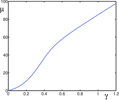
Figure 1: Dimensionless chemical potential $\mu$ as a function of the dimensionless gas parameter $\gamma$.

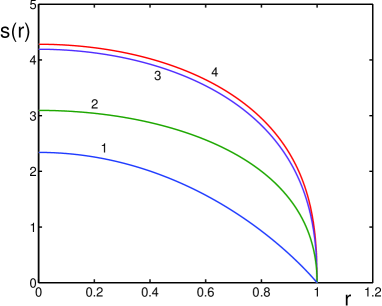
Figure 2: Dimensionless sound velocity $s(r)$, as a function of the spatial variable $r$, for different gas parameters: $\gamma=0.1$ (line 1), $\gamma=0.25$ (line 2), $\gamma=0.5$ (line 3), and $\gamma=1$ (line 4).

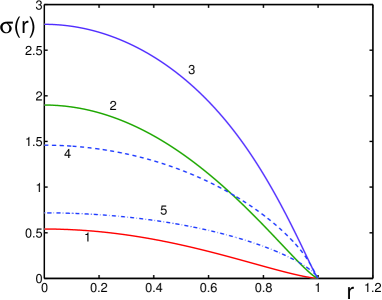
Figure 3: Dimensionless anomalous average $\sigma(r)$, as a function of the spatial variable $r$, for different gas parameters: $\gamma=0.1$ (line 1), $\gamma=0.25$ (line 2), $\gamma=0.5$ (line 3), $\gamma=1$ (line 4), and $\gamma=2$ (line 5).

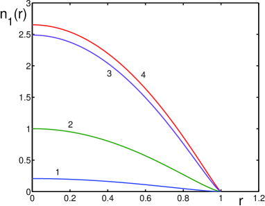
Figure 4: Spatial dependence of the fraction $n_{1}(r)$ of uncondensed atoms for different gas parameters: $\gamma=0.1$ (line 1), $\gamma=0.25$ (line 2), $\gamma=0.5$ (line 3), and $\gamma=1$ (line 4).

A very interesting is the behaviour of the condensate fraction $n_{0}$ as a function of the spatial variable. For small gas parameters $\gamma<0.3$, the condensate fraction exhibits a maximum at the trap center, as in Fig. 5a. While, starting from $\gamma\approx 0.3$, the condensate fraction has a local minimum at the trap center, as in Fig. 5b. This trap-center depletion deepens with the increase of $\gamma$, and the condensate is pushed out of the trap center to its boundary, as is demonstrated in Fig. 6. Such a behaviour of the condensate fraction is in agreement with the Monte Carlo simulations [12, 13].

                 

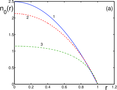
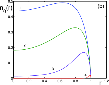
Figure 5: Spatial dependence of the condensate fraction $n_{0}(r)$ for different gas parameters: (a) no trap-center depletion for small $\gamma<0.3$; here $\gamma=0.01$ (line 1), $\gamma=0.1$ (line 2), and $\gamma=0.25$ (line 3); (b) trap-center depletion for $\gamma>0.3$; here $\gamma=0.35$ (line 1), $\gamma=0.4$ (line 2), $\gamma=0.5$ (line 3), and $\gamma=1$ (line 4).

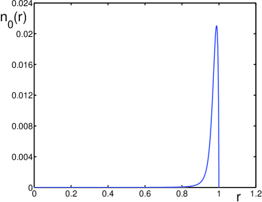
Figure 6: For $\gamma=1$, the condensate fraction is pushed out of the trap center and is located close to the boundary.

The effect of the trap-center depletion is due to the presence in the equation for the condensate fraction (45) of the negative terms, describing the fraction of uncondensed atoms, and the anomalous average. In the Bogolubov approximation, when both these terms are absent, the appearance of the trap-center depletion is impossible, as is evident from equation (45). This effect also does not occur, if one omits the anomalous average, while keeping the fraction of uncondensed atoms, as is illustrated in Fig. 7. This emphasizes the necessity of accurately taking into account the anomalous average that in our case is given by equation (49). Other forms of the anomalous average, which can be met in literature, e.g. in [52, 53], also do not lead to the trap-center depletion.

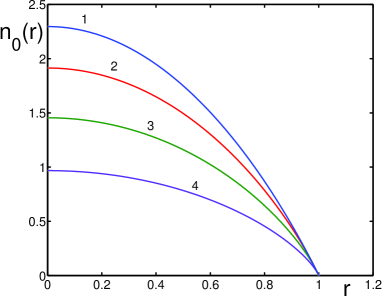
Figure 7: Role of the anomalous average in the effect of trap-center depletion. Omitting in equation (45) the anomalous average results in the spatial behaviour of the condensate fraction with a maximum at the trap center for all gas parameters: $\gamma=0.1$ (line 1), $\gamma=0.25$ (line 2), $\gamma=0.5$ (line 3), and $\gamma=1$ (line 4).

The mean condensate fraction in the trap, defined in equation (53), is presented in Fig. 8, where it is compared with the results of the Bogolubov approximation (BA) [8] and of the diffusion Monte Carlo (DMC) analysis [13] listed in Table 1. The Bogolubov approximation essentially overestimates the condensate fraction for $\gamma<0.5$, but becomes zero at $\gamma=0.654$, where the DMC simulations still show the condensate fraction of $10\%$. The condensate fraction, defined in equation (53), is a bit lower than the DMC results.

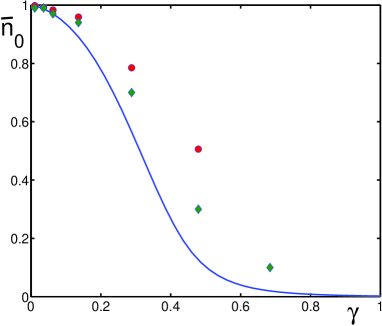
Figure 8: Mean condensate fraction in a trap as a function of the gas parameter (solid line), compared to the Bogolubov approximation (fat dots) and the diffusion Monte Carlo simulation (diamonds).

$\gamma$	$BA$ [8]	$DMC$ [13]
0.011	0.998	0.99
0.036	0.992	0.99
0.063	0.983	0.97
0.136	0.959	0.94
0.288	0.785	0.7
0.479	0.506	0.3
0.684	$-$	0.1

Table 1: Numerical results for the mean condensate fraction of the trapped Bose gas in the Bogolubov approximation (BA) [8] and in the diffusion Monte Carlo (DMC) analysis [13]. For $\gamma=0.684$, the BA predicts a negative condensate fraction.

Although a finite system, corresponding to a trapped Bose-condensed gas, is not the same as a homogeneous superfluid, it is interesting to compare the condensate fractions in these two cases. The atoms of ⁴He at saturated vapor pressure are well represented [49] by hard spheres of diameter $a_{s}=2.203$ Å, which translates into the gas parameter $\gamma=0.59$. The DMC simulations for the related $\gamma$ estimate the condensate fraction of $18\%$. The recent experiments with bulk liquid helium [54, 55] give the zero temperature value $n_{0}=(7.25\pm 0.75)\%$ at saturated vapor pressure and $n_{0}=(2.8\pm 0.2)\%$ at the pressure close to solidification. In our case, for the gas parameter $\gamma=0.59$, we find $n_{0}=4.4\%$.

5 Discussion

We have analyzed the effect of the local condensate trap-center depletion, when for the gas parameter $\gamma>0.3$ the spatial distribution of the condensate fraction exhibits a local minimum at the trap center, contrary to the maximum at the trap center for lower gas parameters $\gamma<0.3$, as has been observed in Monte Carlo simulations [12, 13]. This effect cannot be described by solving the nonlinear Schrödinger equation, either in the Thomas-Fermi approximation or in more refined approximations.

But this effect can be explained employing the self-consistent approach to Bose-condensed systems [16, 21, 22, 23, 26, 39, 40], which is applied here for trapped atoms. In the frame of this approach, we use the Thomas-Fermi approximation. Since the critical gas parameter, when the local-depletion effect develops, is $\gamma\approx 0.3$, one may ask whether the Thomas-Fermi approximation is applicable in this range of $\gamma$. To this end, we remember that the Thomas-Fermi approximation, neglecting the kinetic energy term, is justified, when the interaction energy is much larger than kinetic energy. The interaction energy per atom is of the order $E_{int}\sim\rho\Phi_{0}\sim 4\pi\rho a_{s}/m$. And the effective kinetic energy of an atom is $E_{kin}\sim 1/2ma^{2}\sim\rho^{2/3}/2m$, where $a$ is mean interatomic distance. Therefore, $E_{int}/E_{kin}\sim 8\pi\gamma$. The interaction energy is much larger than the kinetic energy, provided that $\gamma\gg 1/8\pi=0.0398$. The critical value of $\gamma=0.3$ is an order larger than $0.04$, hence for the values of $\gamma$ around $0.3$ and higher, where the local depletion effect arises, the Thomas-Fermi approximation is certainly valid.

The important role in the explanation of the local-depletion effect is played by the existence of the anomalous average, without which the effect does not occur. From the form of the anomalous average (13) it follows that the modulus $|\sigma_{1}(\bf r)|$ of the anomalous average $\sigma_{1}(\bf r)$ defines the density of pair-correlated atoms [16, 26]. In that sense, the anomalous average is connected with pair correlations. The relation of the anomalous average to pair correlations can also be illustrated by considering the two-body scattering matrix [56]

$$S_{k}=\int\Phi({\bf r}-{\bf r}^{\prime})\;\langle\;\varphi_{k}^{*}({\bf r})\varphi_{-k}^{*}({\bf r}^{\prime})\hat{\psi}({\bf r}^{\prime})\hat{\psi}({\bf r})\;\rangle\;d{\bf r}d{\bf r}^{\prime}$$

describing the scattering of two particles from the medium to the momentum states $\varphi_{k}({\bf r})$. With the contact interaction potential (1), the scattering matrix becomes

$$S_{k}=\Phi_{0}\int|\;\varphi_{k}({\bf r})\;|^{2}\left[\eta^{2}({\bf r})+\sigma_{1}({\bf r})\right]\;d{\bf r}\;,$$

where the Bogolubov shift (3) is used and the anomalous average is defined in equation (13). Although the physical origin of the effect is rather clear, as being due to strong interatomic interactions pushing the condensate out of the trap center, but its theoretical description is quite delicate, requiring an accurate description of the anomalous average.

One more question that can arise when analyzing the results of the calculations, is whether strong atomic interactions push uncondensed atoms from the trap center? To the first glance, looking at Fig. 4, one does not see a spreading of uncondensed atoms from the trap center under increasing interactions. However, one should not forget that in the figures we use the dimensionless units. While in dimensional form the atomic cloud radius depends on the interaction strength as

$$r_{TF}=\sqrt{\frac{2\mu_{0}}{m\omega_{0}^{2}}}\;\approx\;\left(15\;\frac{a_{s}}{l_{0}}\;N\right)^{1/5}\;l_{0}\;.$$

Therefore, under strengthening interactions, that is increasing the scattering length $a_{s}$, the cloud radius also increases. In that sense, atomic interactions do push atoms out of the trap center. Then the cloud shape becomes more flat. But the maximal density of uncondensed atoms remains at the trap center because normal atoms always prefer to gather at the location of the minimal external potential, just spreading in space by enlarging the cloud size for reducing their density and interaction energy. Notice that employing dimensional quantities, we would have to fix two additional parameters, the trap oscillator frequency $\omega_{0}$ and the number of atoms $N$. While the scaling we have employed requires just the single gas parameter $\gamma$, which makes the consideration essentially more general.

The found threshold gas parameter $\gamma=0.3$ for the occurrence of the trap-center depletion of condensed atoms is in agreement with the Monte Carlo analysis [13]. The mean condensate fraction as a function of the gas parameter is close to the dependence found in Monte Carlo simulations.

References

- [1] Pethick C J and Smith H 2008 Bose-Einstein Condensation in Dilute Gases (Cambridge: Cambridge University)
- [2] Bloch I, Dalibard J and Zwerger W 2008 Rev. Mod. Phys. 80 885
- [3] Yurovsky V A, Olshanii M and Weiss D S 2008 Adv. At. Mol. Opt. Phys. 55 61
- [4] Krems R V, Friedrich B and Stwalley W C (eds.) 2009 Cold Molecules: Theory, Experiment, Applications (Boca Raton: CRC Press)
- [5] Cote R, Gould P L, Rozman M G and, Smith W W (eds.) 2009 Pushing the Frontiers of Atomic Physics (Singapore: World Scientific)
- [6] Bogolubov N N 1947 J. Phys. (Moscow) 11 23
- [7] Xu K, Liu Y, Miller D E, Chin J K, Setiawan W and Ketterle W 2006 Phys. Rev. Lett. 96 180405
- [8] Javanainen J 1996 Phys. Rev. A 54 3722
- [9] Yukalov V I, Yukalova E P and Bagnato V S 2002 Phys. Rev. A 66 043602
- [10] Yukalov V I, Yukalova E P and Gluzman S 1998 Phys. Rev. A 58 96
- [11] Yukalov V I, Yukalova E P and Bagnato V S 2002 Phys. Rev. A 66 025602
- [12] DuBois J L and Glyde H R 2001 Phys. Rev. A 63 023602
- [13] DuBois J L and Glyde H R 2003 Phys. Rev. A 68 033602
- [14] Ziegler K and Shukla A 1997 Phys. Rev. A 56 1438
- [15] Proukakis N P and Jackson B 2008 J. Phys. B 41 203002
- [16] Yukalov V I 2016 Laser Phys. 26 062001
- [17] Griesmaier A 2007 J. Phys. B 40 R91
- [18] Baranov M A 2008 Phys. Rep. 464 71
- [19] Baranov M A, Dalmonte M, Pupillo G and Zoller P 2012 Chem. Rev. 112 5012
- [20] Gadway B and Yan B 2016 J. Phys. B 49 152002
- [21] Yukalov V I 2005 Phys. Rev. E 72 066119
- [22] Yukalov V I 2006 Phys. Lett. A 359 712
- [23] Yukalov V I 2008 Ann. Phys. (N.Y.) 323 461
- [24] Lieb E H, Seiringer R, Solovej J P and Yngvason J 2005 The Mathematics of the Bose Gas and its Condensation (Basel: Birkhäuser)
- [25] Yukalov V I 2007 Laser Phys. Lett. 4 632
- [26] Yukalov V I 2011 Phys. Part. Nucl. 42 460
- [27] Bogolubov N N 1967 Lectures on Quantum Statistics vol 1 (New York: Gordon and Breach)
- [28] Bogolubov N N 1970 Lectures on Quantum Statistics vol 2 (New York: Gordon and Breach)
- [29] Bogolubov N N 2015 Quantum Statistical Mechanics (Singapore: World Scientific)
- [30] Yukalov V I 2006 Laser Phys. 16 511
- [31] Yukalov V I 2013 Laser Phys. 23 062001
- [32] Hugenholtz N M and Pines D 1959 Phys. Rev. 116 489
- [33] Hohenberg P C and Martin P C 1965 Ann. Phys. (N.Y.) 34 291
- [34] Purwanto W and Zhang S 2005 Phys. Rev. A 72 053610
- [35] Gotlibovych I, Schmidutz T F, Gaunt A L, Navon N, Smith R P and Hadzibabic Z 2014 Phys. Rev. A 89 061604
- [36] Giorgini S, Boronat J and Casulleras J 1999 Phys. Rev. A 60 5129
- [37] Pilati S, Sakkos K, Boronat J, Casulleras J and Giorgini S 2006 Phys. Rev. A 74 043621
- [38] Rossi M and Salasnich L 2013 Phys. Rev. A 88, 053617
- [39] Yukalov V I and Yukalova E P 2014 Phys. Rev. A 90 013627
- [40] Yukalov V I and Yukalova E P 2014 J. Phys B 47 095302
- [41] Matsubara T and Matsuda K 1956 Prog. Theor. Phys. 16 569
- [42] Floerchinger S and Wetterich C 2009 Phys. Rev. A 79 063602
- [43] Andersen J O 2004 Rev. Mod. Phys. 76 599
- [44] Yukalov V I 2004 Laser Phys. Lett. 1 435
- [45] Yukalov V I 2017 Laser Phys. Lett. 14 073001
- [46] Kim H, Kim C S, Huang C L, Song H S and Yi X X 2012 Phys. Rev. A 85 033611
- [47] Kim H, Kim C S, Huang C L, Song H S and Yi X X 2012 Phys. Rev A 85 053629
- [48] Yukalov V I 2016 Phys. Rev. E 94 012106
- [49] Kalos M H, Levesque D and Verlet L 1974 Phys. Rev. A 9 2178
- [50] Olshani M and Pricoupenko L 2002 Phys. Rev. Lett. 88 010402
- [51] Caracanhas M A, Seman J A, Ramos E R F, Henn E A I, Magalhaes K M F, Helmerson K and Bagnato V S 2009 J. Phys. B 42 145304
- [52] Boudjemâa A and Benarous M 2011 Phys. Rev. A 84 043633
- [53] Boudjemâa A and Guebli N 2017 J. Phys. A 50 425004
- [54] Glyde H R, Diallo S O, Azuah R T, Kirichek O and Taylor J W 2011 Phys. Rev. B 84 184506
- [55] Diallo S O, Azuah R T, Abernathy D L, Rota R, Boronat J and Glyde H R 2012 Phys. Rev. B 85 140505
- [56] Bogolubov N N, Logunov A A and Todorov I T 1975 Introduction to Axiomatic Quantum Field Theory (London: Benjamin)