DJAM: distributed Jacobi asynchronous method for learning personal models

Abstract

Processing data collected by a network of agents often boils down to solving an optimization problem. The distributed nature of these problems calls for methods that are, themselves, distributed. While most collaborative learning problems require agents to reach a common (or consensus) model, there are situations in which the consensus solution may not be optimal. For instance, agents may want to reach a compromise between agreeing with their neighbors and minimizing a personal loss function. We present DJAM, a Jacobi-like distributed algorithm for learning personalized models. This method is implementation-friendly: it has no hyperparameters that need tuning, it is asynchronous, and its updates only require single-neighbor interactions. We prove that DJAM converges with probability one to the solution, provided that the personal loss functions are strongly convex and have Lipschitz gradient. We then give evidence that DJAM is on par with state-of-the-art methods: our method reaches a solution with error similar to the error of a carefully tuned ADMM in about the same number of single-neighbor interactions.

I Learning personal models

Consider $n$ agents, each with a personal loss function: $f_{i}:{\mbox{\bf R}}^{p}\rightarrow{\mbox{\bf R}}$, $\theta_{i}\mapsto f_{i}(\theta_{i})$, for agent $i=1,\ldots,n$. For example, $f_{i}(\theta_{i})$ could be the loss of a model parameterized by $\theta_{i}$ on agent $i$’s personal dataset. The agents are the nodes of an undirected, connected network.

Each agent aims to find a model that minimizes both the mismatch with its neighbors’ models and its personal loss. More specifically, agents aim to solve

$$\min_{\theta_{1},\ldots,\theta_{n}}\hskip 11.38092pt\frac{1}{2}\sum_{i<j}^{n}W_{ij}\|\theta_{i}-\theta_{j}\|^{2}+\sum_{i=1}^{n}f_{i}(\theta_{i}),$$ (1)

where $W=\left(W_{ij}\right)\in{\mbox{\bf R}}^{n\times n}$ is a symmetric matrix that mirrors the topology of the network: $W_{ij}~{}\geq~{}0$ if agents $i$ and $j$ are connected in the network; $W_{ij}=0$ otherwise. The weight $W_{ij}$ controls the degree of agreement we want between agents $i$ and $j$: a larger $W_{ij}$ enforces more similarity between the corresponding agents’ models.

Problem (1) can model a number of applications, including peer-network recomender systems, distributed (linear) classification [1], opinion propagation, and field estimation [2]; the latter is discussed in Section IV. The weights $W_{ij}$ may be chosen, for instance, based on the spatial distance between pairs of agents, or according to the similarity of their personal datasets.

Closest related works. Optimization problem (1) has been addressed in [1]. For convex loss functions $f_{i}$ that are quadratic, the authors suggest a distributed algorithm, which we refer to as Model Propagation Algorithm (MPA). In each round of MPA, an agent wakes up at random, interacts with one of its neighbours, and both go back to sleep; the pattern repeats for the following rounds. MPA is an algorithm that is easy to implement because it is asynchronous (each agent has its own clock to wake up), has no parameter to tune, and involves only single-neighbour interactions (the agent that wakes up does not need to coordinate message-passing with several neighbours). The authors in [1] prove that MPA converges to the solution of (1) in expectation (mean-value), for quadratic loss functions; for these functions, the iterations of the method we propose coincide with those of MPA. For more general loss functions, those authors suggest a different algorithm, based on ADMM, which needs parameter tuning to reach optimal performance. This ADMM-based algorithm for collaborative learning (CL-ADMM), will be compared with our algorithm in Section IV.

Problem (1), with the same kind of asynchronous single-neighbour interactions, can also be tackled by the algorithm proposed in [2]. In the language of [2], this corresponds to having agents deviate from the “rational” decision at each round (the rational decision would require each agent to interact will all its neighbors). For such “irrational” decisions, the authors show that, with probability one, the iterations of their algorithm will visit infinitely often a neighborhood of the solution of (1), although the iterations may continually escape that neighborhood. Finally, a recent follow-up on [1] is [3], where a block coordinate descent method with broadcast communications is used to solve problem (1).

Contributions. We show that a simple Jacobi-like distributed algorithm, which we call DJAM, can solve (1) with the same kind of asynchronous single-neighbor interactions. DJAM, which can also be seen as a randomized block-coordinate method, has no parameters that need tuning. For continuously differentiable personal loss functions that are strongly convex and have Lipschitz gradient, that is, such that, for all $i$,

$$(\nabla f_{i}(x)-\nabla f_{i}(y))^{T}(x-y)\geq m_{i}\|x-y\|^{2}$$ (2)

for some $m_{i}>0$ and all $x,y$, and

$$\|\nabla f_{i}(x)-\nabla f_{i}(y)\|\leq M_{i}\|x-y\|$$ (3)

for some $M_{i}\geq 0$ and all $x,y$, we show that DJAM converges to the solution of (1) with probability one. The values of $m_{i}$ and $M_{i}$ are used for proving convergence but need not be known when implementing DJAM.

DJAM improves on MPA not only because it applies to a larger class of functions than quadratics, but also because it converges in a stronger sense: as the proof of Theorem 1 ahead shows, the DJAM iterations are uniformly bounded; thus, the convergence in expectation in [1] follows by the dominated convergence theorem from our convergence with probability one. Our result only applies to a (somewhat) more restricted class of functions than the one of [2], but our convergence mode is stronger than the one of [2]. Also, unlike in [3], our method does not require knowing the values of $M_{i}$ upon implementation.

Other related work. Although [1, 2] are the closest works that we are aware of, many other distributed algorithms solve variations of problem (1). We now mention some representative work.

A number of distributed algorithms allow agents to solve an underlying optimization problem by reaching consensus on the solution. They use techniques ranging from distributed (sub)gradient descent [4], [5] to more elaborate techniques such as EXTRA [6], distributed ADMM [7, 8], dual averaging [9], and distributed Augmented Lagrangean (AL) [10]. Some algorithms aim at more specific optimization tasks such as distributed lasso regression [11], distributed SVMs [12], and distributed RFVL networks [13]. All of these methods aim at reaching consensus solutions—all agents converge to the same value. Conversely, in problem (1), agents want to find different (personalized) values.

The related problem of network lasso is dealt with in [14]; however, the cost in [14] puts a strong emphasis on neighbouring models being exactly equal, whereas in our case we want them to be similar, but not necessarily equal. The methods proposed in [15] and [16] can tackle more general problems, but both require that agents communicate with all their neighbors before updating, while our method needs only communications between two agents at a time. Problem (1) is also referred to as multitask problem; this problem is solved in [17] for a more restricted class of personal losses than ours.

II DJAM

A naive Jacobi-like approach to solve (1) would work as follows: at each round $t$, one agent $i$, picked at random, would update its model according to

$$\theta_{i}(t+1)=\arg\min_{\theta_{i}}\frac{1}{2}\sum_{k\in\mathcal{N}_{i}}W_{ik}\|\theta_{i}-\theta_{k}(t)\|^{2}+f_{i}(\theta_{i}),$$

where ${\mathcal{N}}_{i}$ is the set of neighbors of agent $i$. This naive approach, however, has a major drawback: it requires that agent $i$ communicates with all its neighbors—to receive their up-to-date models $\theta_{k}(t)$—before updating its own model. Coordinating such message-passing, at each round, is cumbersome. A lighter scheme, involving only a single pair of agents at a time, is simpler to implement in practice, and requires fewer communications, at the expense of slowing down convergence.

The key idea, which we borrow from [1], is to have each agent $i$ keep its own model $\Theta_{i}^{i}$ as well as (often outdated) versions of its neighbors’ models, $\Theta_{i}^{k}$ for $k\in\mathcal{N}_{i}$. The versions of each pair of neighbors are updated whenever they communicate with each other. More specifically, at each round $t$, agent $i$ wakes up and chooses a neighbor $j\in\mathcal{N}_{i}$ to communicate with. They begin by exchanging information on their models, meaning that $\Theta_{i}^{j}(t+1)=\Theta_{j}^{j}(t)$ and $\Theta_{j}^{i}(t+1)=\Theta_{i}^{i}(t)$. All other variables remain unchanged. Afterwards, both agents update their own model via

$$\Theta_{l}^{l}(t+1)=\arg\min_{\theta_{l}}\frac{1}{2}\sum_{k\in\mathcal{N}_{l}}W_{lk}\|\theta_{l}-\Theta_{l}^{k}(t+1)\|^{2}+f_{l}(\theta_{l})$$ (4)

for $l\in\{i,j\}$.

For the purpose of analyzing DJAM, we merge these two steps into a single one. Since the personal model $\Theta_{i}^{i}$ can be created at any time at agent $i$ via (4), it need not be stored. This means that, at round $t$ of DJAM, two neighboring agents $i$ and $j$ will compute and share their own models with each other:

$$\Theta_{i}^{j}(t+1)=\arg\min_{\theta_{j}}\frac{1}{2}\sum_{k\in\mathcal{N}_{j}}W_{jk}\|\theta_{j}-\Theta_{j}^{k}(t)\|^{2}+f_{j}(\theta_{j}),$$ (5)

and similarly for $\Theta_{j}^{i}$. Mind that the right-hand side of (5) is computed by agent $j$ and sent to agent $i$, who stores the result in the variable on the left-hand side of (5).

III Proof of convergence for DJAM

We now prove that DJAM, the algorithm with updates given by (5), converges with probability one to the solution of (1). We omit some laborious (but otherwise painless) technical steps that would make the notation and proofs too lengthy.

Let ${\mathcal{E}}$ be the set of edges of the network that links the agents. The network need not be fully connected: each agent is connected only to a subset of the remaining agents. We assume that at each round (A1) one edge of ${\mathcal{E}}$ is chosen at random, independently of previous choices; and (A2) each edge in $\mathcal{E}$ has a fixed, positive probability of being chosen. It is easy to verify that, under assumptions (A1) and (A2), each edge in $\mathcal{E}$ is chosen infinitely often with probability one.

The number of times a given edge $(i,j)$ is chosen between rounds $s$ and $t$ (with $s\leq t$) is a random variable defined as $S_{(i,j)}(s,t):=\sum_{\tau=s}^{t}Y_{(i,j)}(\tau)$, where $Y_{(i,j)}(\tau)=1$ if edge $(i,j)$ is chosen at round $\tau$, and zero otherwise. We now define a useful family of stopping times $\left(T_{m}\right)_{m\geq 0}$. We let $T_{0}:=0$ and, for $m\geq 0$,

$$T_{m+1}\mathrel{\vbox{\hbox{\scriptsize.}\hbox{\scriptsize.}}}=\min\left\{t\mid S_{(i,j)}(T_{m}+1,t)\geq 1,\forall(i,j)\in\mathcal{E}\right\}.$$

In words, $T_{m+1}$ is the first round after $T_{m}$ by which all edges have been chosen at least once. Assumptions (A1) and (A2) imply that any $T_{m}$ is finite for any $m$. Addtionally, $T_{m}\rightarrow\infty$ as $m\rightarrow\infty$ with probability one.

We first state an important consequence of assumptions (2) and (3) on each personal loss function $f_{j}$.

Lemma 1.

Let $w_{j}\mathrel{\vbox{\hbox{\scriptsize.}\hbox{\scriptsize.}}}=\sum_{k\in\mathcal{N}_{j}}W_{jk}$, and take the function $F_{j}(x)=f_{j}(x)+\frac{1}{2}w_{j}\|x\|^{2}$. Note that $\nabla F_{j}$ is a bijective map (with inverse map $(\nabla F_{j})^{-1}$) because, from standard convex theory, $\nabla f_{j}$ is. Then, for any $a$ and $b$,

$$\|(\nabla F_{j})^{-1}(a)-(\nabla F_{j})^{-1}(b)\|\leq\left(m_{j}+w_{j}\right)^{-1}\|a-b\|.$$

Proof.

Choose $x=(\nabla F_{j})^{-1}(a)$ and $y=(\nabla F_{j})^{-1}(b)$. Clearly, $a-b=(\nabla f_{j}(x)-\nabla f_{j}(y))+w_{j}(x-y)$. Multiplying both sides of this equality by $(x-y)^{T}$ yields $(x-y)^{T}(a-b)\geq(m_{j}+w_{j})\|x-y\|^{2}$, where the inequality is due to the strong convexity of $f_{j}$, property (2). By the Cauchy-Schwartz inequality, $\|x-y\|\|a-b\|\geq(x-y)^{\top}(a-b)$, and, thus, $\|x-y\|\|a-b\|\geq(m_{j}+w_{j})\|x-y\|^{2}$. Inserting the definitions of $x$ and $y$ yields $\|a-b\|\geq(m_{j}+w_{j})\left\|(\nabla F_{j})^{-1}(a)-(\nabla F_{j})^{-1}(b)\right\|$. ∎

We now give our main convergence result.

Theorem 1 (DJAM converges with probability one).

Let $\Theta^{*}=(\Theta_{1}^{*},\ldots,\Theta_{n}^{*})$ be the solution of (1). Let $\Theta_{i}^{j}(t+1)$, $i=1,\ldots,n$, $j\in\mathcal{N}_{i}$, be updated via (5) whenever edge $(i,j)$ is chosen at round $t$, and similarly for $\Theta_{j}^{i}(t+1)$. Then, for any pair of agents $(i,j)$, $\Theta_{i}^{j}(t)\rightarrow\Theta_{j}^{*}$ as $t\rightarrow\infty$, with probability one.

Proof.

Let $F_{j}$, and $w_{j}$ be defined as in Lemma 1. Suppose edge $(i,j)$ is chosen at time $t$. It can be verified from (5) and from the first order condition for optimality that $\Theta_{i}^{j}(t~{}+~{}1)~{}=~{}(\nabla F_{j})^{-1}\left(\sum_{k\in\mathcal{N}_{j}}W_{jk}\Theta_{j}^{k}(t)\right)$, where $F_{j}$ is as defined in Lemma 1; similarly, we have that $\Theta_{j}^{*}=(\nabla F_{j})^{-1}\left(\sum_{k\in\mathcal{N}_{j}}W_{jk}\Theta_{k}^{*}\right)$ for each component of the solution.

Lemma 1 allows us to find that

$$\|\Theta_{i}^{j}(t+1)-\Theta_{j}^{*}\|$$ (6)

$$\leq (m_{j}+w_{j})^{-1}\|\sum W_{jk}(\Theta_{j}^{k}(t)-\Theta_{k}^{*})\|$$

$$\leq (m_{j}+w_{j})^{-1}\sum W_{jk}\|\Theta_{j}^{k}(t)-\Theta_{k}^{*}\|$$

$$\leq (m_{j}+w_{j})^{-1}w_{j}\max_{k}\|\Theta_{j}^{k}(t)-\Theta_{k}^{*}\|$$

$$\leq (m_{j}+w_{j})^{-1}w_{j}V(t),$$

where $V(t):=\max_{l,k}\|\Theta_{l}^{k}(t)-\Theta_{k}^{*}\|$ is the maximum error at round $t$ between the agents’ estimates and the solution.

If edge $(i,j)$ is chosen at round $t$, we have, by the derivation above, that

$$\|\Theta_{i}^{j}(t+1)-\Theta_{j}^{*}\|\leq V(t).$$ (7)

If that edge is not chosen, then $\Theta_{i}^{j}(t+1)=\Theta_{i}^{j}(t)$ and, by definition of $V(t)$, $\|\Theta_{i}^{j}(t+1)-\Theta_{j}^{*}\|\leq V(t)$. We conclude that (7) holds for any pair $(i,j)$ and, so, $V(t+1)~{}\leq~{}V(t)$. Since $V(t)\geq 0$, the limit (which is a random variable) $V\mathrel{\vbox{\hbox{\scriptsize.}\hbox{\scriptsize.}}}=\lim_{t\rightarrow\infty}V(t)$ is thus always well defined. The goal of the proof is to show that $V=0$ with probability one.

Recall that $T_{m+1}$ denotes the first round after $T_{m}$ by which all edges were selected at least once. It should be clear to the reader that the remainder of the proof holds almost surely, since $T_{m}$ is finite for all $m$ with probability one. Suppose edge $(i,j)$ was selected at round $T_{m}+s$. Then

$$\|\Theta_{i}^{j}(T_{m}+s)-\Theta_{j}^{*}\|\leq(m_{j}+w_{j})^{-1}w_{j}V(T_{m}),$$ (8)

cf. inequality (6). Since, by definition of $T_{m}$ and $T_{m+1}$, all edges $(i,j)$ in the graph were selected at least once between $T_{m}$ and $T_{m+1}$, inequality (8) holds for all $(i,j)\in\mathcal{E}$ when $T_{m}+s=T_{m+1}$. In other words,

$$\|\Theta_{i}^{j}(T_{m+1})-\Theta_{j}^{*}\|\leq(m_{j}+w_{j})^{-1}w_{j}V(T_{m})$$

for all edges $(i,j)\in\mathcal{E}$. It follows, by the definition of $V(T_{m+1})$, that

$$V(T_{m+1})\leq\beta V(T_{m}),$$ (9)

where $\beta~{}\mathrel{\vbox{\hbox{\scriptsize.}\hbox{\scriptsize.}}}=~{}\max_{i}\ \{(m_{i}+w_{i})^{-1}w_{i}\}\in[0,1)$.

Let us take the limit $m\rightarrow\infty$ in (9). We know that $T_{m}\rightarrow\infty$, and it follows from (9) that $V\leq\beta V$. Thus, owing to $0\leq\beta<1$, we must have $V=0$, which implies $\Theta_{i}^{j}(t)\rightarrow\Theta_{j}^{*}$ as $t\rightarrow\infty$, for any $(i,j)$. ∎

Inequality (9) implies that $V(t)\leq V(0)$. The iterations $\left(\Theta_{k}^{l}(t)\right)_{t\geq 0}$ are, thus, uniformly bounded. We conclude (by the dominated convergence theorem) that our result implies the convergence in expectation result in [1].

IV Field estimation example

Setup. Following [2], we consider a field estimation setup that leads to a problem of the form (1). The $n$ agents are spread in a region and wish to profile a certain quantity, say, temperature, over the region: agent $i$ cares only about the value of the quantity at its location, $\theta_{i}$. Assume that the true values of the temperatures, $\theta=(\theta_{1},\ldots,\theta_{n})$, are drawn from a prior distribution: a normal distribution with known mean and covariance $\Sigma$; as in [2], we assume that the off-diagonal elements of $\Sigma^{-1}$ match the sparsity of the network, that is, $(\Sigma^{-1})_{ij}>0$ if and only if $(i,j)\in\mathcal{E}$. Agent $i$ measures $y_{i}=\theta_{i}+\nu_{i}$, where $\nu_{i}$ models identically distributed sensor noise (for simplicity), which is independent across agents.

MAP estimation. A maximum a posteriori (MAP) approach seeks the $\theta=(\theta_{1},\ldots,\theta_{n})$ that maximizes $\sum_{i=1}^{n}\log\mathop{\bf Prob}(y_{i}\mid\theta_{i})+\log\mathop{\bf Prob}(\theta_{1},\ldots,\theta_{n})$; or, equivalently, the $\theta$ that minimizes

$$\frac{1}{2}\left(\sum_{i\sim j}\sigma_{ij}(\theta_{i}-\theta_{j})^{2}+\sum_{i=1}^{n}\sigma_{ii}\theta_{i}^{2}\right)+\sum_{i=1}^{n}\phi(y_{i}-\theta_{i}),$$ (10)

where $\sigma_{ij}:=(\Sigma^{-1})_{ij}$ and $\phi$ depends on the distribution of the noise $\nu_{i}$. We let $\phi$ be a Huber penalty function to handle outliers [18]. Finally, defining the personal loss functions as $f_{i}(\theta_{i})\mathrel{\vbox{\hbox{\scriptsize.}\hbox{\scriptsize.}}}=\phi(y_{i}-\theta_{i})+\frac{1}{2}\sigma_{ii}\theta_{i}^{2}$ puts (10) in the form (1). Also, assumptions (2) and (3) hold.

Results: comparing DJAM with CL-ADMM. Since the algorithm MPA from [1] applies only to quadratic functions, we use the ADMM-based algorithm CL-ADMM from [1] to compare with DJAM. Note that both CL-ADMM and DJAM converge to the solution with probability one. The algorithm CL-ADMM, however, being based on ADMM, has a parameter to tune—the parameter in the quadratic penalization part of the augmented Lagrangian function. This parameter, which we refer to as $\rho$, is known to affect noticeably the convergence speed of ADMM.

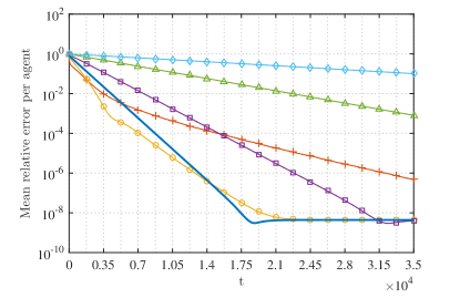
Figure 1: Mean relative error $\left(\left\|\Theta_{i}^{i}(t)-\Theta_{i}^{*}\right\|/\left\|\Theta_{i}^{*}\right\|\right)$ per agent on the smooth field estimation problem for an instance with $n=30$ agents; the mean was obtained by averaging over 100 Monte Carlo trials. Our method, DJAM, corresponds to the blue line with no markers. The other lines correspond to CL-ADMM with $\rho$ equal to 0.1 (red $+$), 0.316 (yellow $\ocircle$), 1.0 (violet $\square$), 3.16 (green $\vartriangle$), and 10 (cyan $\lozenge$). All methods stop improving after reaching a relative error slightly above $10^{-9}$, which we believe is due to rounding errors.

The results for a field estimation instance are shown in Figure 1. It shows, across rounds $t$, the relative error between an agent’s private model $\Theta_{i}^{i}(t)$ and the solution component $\Theta_{i}^{*}$: $\left\|\Theta_{i}^{i}(t)-\Theta_{i}^{*}\right\|/\left\|\Theta_{i}^{*}\right\|$. The relative error was averaged over agents and over 100 Monte Carlo trials where, in each Monte Carlo run, we choose a different set of edges along time.

Figure 1 confirms that the speed of convergence of CL-ADMM varies with the parameter $\rho$ noticeably. In fact, we verified in other simulations (omitted due to lack of space) that the optimal $\rho$ varied significantly with the number of agents, with the range of values for $\sigma_{ij}$, and with the noise distribution—we found the optimal $\rho$ for those simulations by careful hand-tuning. In contrast, DJAM is on par with the best $\rho$ in Figure 1, and needs no parameter tuning.

References

- [1] P. Vanhaesebrouck, A. Bellet, and M. Tommasi, “Decentralized collaborative learning of personalized models over networks,” in Proceedings of the 20th International Conference on Artificial Intelligence and Statistics (A. Singh and J. Zhu, eds.), vol. 54 of Proceedings of Machine Learning Research, (Fort Lauderdale, FL, USA), pp. 509–517, PMLR, 20–22 Apr 2017.
- [2] C. Eksin and A. Ribeiro, “Distributed network optimization with heuristic rational agents,” IEEE Transactions on Signal Processing, vol. 60, pp. 5396–5411, Oct 2012.
- [3] A. Bellet, R. Guerraoui, M. Taziki, and M. Tommasi, “Personalized and private peer-to-peer machine learning,” in International Conference on Artificial Intelligence and Statistics, AISTATS 2018, 9-11 April 2018, Playa Blanca, Lanzarote, Canary Islands, Spain, pp. 473–481, 2018.
- [4] K. Kvaternik and L. Pavel, “Lyapunov analysis of a distributed optimization scheme,” in International Conference on NETwork Games, Control and Optimization (NetGCooP 2011), pp. 1–5, Oct 2011.
- [5] A. Nedić and A. Ozdaglar, “Distributed subgradient methods for multi-agent optimization,” IEEE Transactions on Automatic Control, vol. 54, no. 1, pp. 48–61, 2009.
- [6] W. Shi, Q. Ling, G. Wu, and W. Yin, “EXTRA: An exact first-order algorithm for decentralized consensus optimization,” SIAM Journal on Optimization, vol. 25, no. 2, pp. 944–966, 2015.
- [7] S. Boyd, N. Parikh, E. Chu, B. Peleato, and J. Eckstein, “Distributed optimization and statistical learning via the alternating direction method of multipliers,” Foundations and Trends® in Machine Learning, vol. 3, no. 1, pp. 1–122, 2011.
- [8] E. Wei and A. Ozdaglar, “On the O(1/k) convergence of asynchronous distributed alternating direction method of multipliers,” IEEE Global Conference on Signal and Information Processing (GlobalSIP), 2013.
- [9] I. Colin, A. Bellet, J. Salmon, and S. Clémençon, “Gossip dual averaging for decentralized optimization of pairwise functions,” in Proceedings of the 33rd International Conference on International Conference on Machine Learning - Volume 48, ICML’16, pp. 1388–1396, JMLR.org, 2016.
- [10] D. Jakovetić, J. M. F. Moura, and J. M. F. Xavier, “Linear convergence rate of a class of distributed augmented lagrangian algorithms,” IEEE Transactions on Automatic Control, vol. 60, no. 4, pp. 922–936, 2015.
- [11] G. Mateos, J. A. Bazerque, and G. B. Giannakis, “Distributed sparse linear regression,” IEEE Trans. Signal Processing, vol. 58, no. 10, pp. 5262–5276, 2010.
- [12] P. A. Forero, A. Cano, and G. B. Giannakis, “Consensus-based distributed support vector machines,” J. Mach. Learn. Res., vol. 11, pp. 1663–1707, Aug. 2010.
- [13] S. Scardapane, D. Wang, M. Panella, and A. Uncini, “Distributed learning for random vector functional-link networks,” Information Sciences, vol. 301, pp. 271 – 284, 2015.
- [14] D. Hallac, J. Leskovec, and S. Boyd, “Network lasso: Clustering and optimization in large graphs,” in International Conference on Knowledge Discovery & Data Mining, KDD: proceedings / International Conference on Knowledge Discovery & Data Mining, pp. 387–396, 2015.
- [15] F. Facchinei, G. Scutari, and S. Sagratella, “Parallel selective algorithms for nonconvex big data optimization,” IEEE Transactions on Signal Processing, vol. 63, pp. 1874–1889, April 2015.
- [16] I. Necoara and D. Clipici, “Parallel random coordinate descent method for composite minimization: Convergence analysis and error bounds,” SIAM Journal on Optimization, vol. 26, no. 1, pp. 197–226, 2016.
- [17] J. Chen, C. Richard, and A. H. Sayed, “Multitask diffusion adaptation over networks,” IEEE Transactions on Signal Processing, vol. 62, pp. 4129–4144, Aug 2014.
- [18] P. Huber, J. Wiley, and W. InterScience, Robust statistics. Wiley New York, 1981.