Antigravity from a spacetime defect

Abstract

We argue that there may exist spacetime defects embedded in Minkowski spacetime, which have negative active gravitational mass. One such spacetime defect then repels a test particle, corresponding to what may be called “antigravity.”

I Introduction

It is possible that a “quantum-spacetime” phase has given rise to the classical spacetime of the present Universe. If that is the case, then it is also possible that there have appeared small imperfections in the emerging classical spacetime. These remnant imperfections may be called “spacetime defects,” by analogy with defects in an atomic crystal.

We have studied a soliton-type spacetime defect which has nontrivial topology for both the spacetime manifold and the matter-field configuration. Specifically, we have constructed a new type of Skyrmion classical solution Klinkhamer2014-prd , for which the nontrivial topology of the $SO(3)$ matter field matches the nontrivial topology of space [essentially $\mathbb{R}P^{3}\sim SO(3)$].

Even before the final soliton was constructed, there were hints that the soliton could have an unusual asymptotic property, namely, a negative active gravitational mass Klinkhamer2013 . This was confirmed by a detailed numerical analysis Guenther2017 . The goal, now, is to understand the origin of this negative gravitational mass.

II Theory and Ansätze

The details of the spacetime manifold and matter fields of the Skyrmion spacetime defect solution have been given in Sec. II of Ref. Klinkhamer2014-prd , which also contains further references. Here, we recall the main results, mainly in order to establish our notation.

The four-dimensional spacetime manifold has the topology

$$M_{4} = \mathbb{R}\times M_{3}\,,$$ (1a)

$$M_{3} = \mathbb{R}P^{3}-p_{\infty}\,,$$ (1b)

where $p_{\infty}$ corresponds to the “point at spatial infinity.”

A particular covering of the manifold $M_{3}$ uses three charts of coordinates, labeled by $n=1,\,2,\,3$. The explicit coordinate charts are discussed in Sec. 2 and App. A of Ref. Klinkhamer2014-mpla . These three sets of coordinates $(X_{n},\,Y_{n},\,Z_{n})$ are invertible and infinitely-differentiable functions of each other in their respective overlap regions (details and further results can be found in Chap. 5 of Ref. Schwarz2010 and a brief summary appears in Sec. 2.1.2 of Ref. Guenther2017 ). At this moment, we will focus on the $n=2$ chart, the other charts being similar. Specifically, the chart-2 coordinates have the following ranges:

$$X_{2}\in(0,\,\pi)\,,\quad Y_{2}\in(-\infty,\,\infty)\,,\quad Z_{2}\in(0,\,\pi)\,,$$ (2)

where $Y_{2}=0$ gives the position of the defect surface (an $\mathbb{R}P^{2}$ submanifold). Henceforth, we will drop the suffix $2$.

The action reads ($c=\hbar=1$)

$$S = \int_{M_{4}}d^{4}X\,\sqrt{-g}\,\Bigg{[}\frac{1}{16\pi G_{N}}\>R+\frac{f^{2}}{4}\>\text{tr}\Big{(}\omega_{\mu}\,\omega^{\mu}\Big{)}+\frac{1}{16e^{2}}\>\text{tr}\Big{(}\left[\omega_{\mu},\,\omega_{\nu}\right]\left[\omega^{\mu},\,\omega^{\nu}\right]\Big{)}\Bigg{]},$$ (3a)

$$\omega_{\mu} \equiv \Omega^{-1}\,\partial_{\mu}\,\Omega\,,$$ (3b)

in terms of the Ricci curvature scalar $R$ and the scalar field $\Omega(X)\in SO(3)$, together with the definition $g\equiv\det g_{\mu\nu}$. In addition to having Newton’s gravitational coupling constant $G_{N}$, there is an energy scale $f$ from the kinetic matter term in (3a). Furthermore, the quartic Skyrme term comes with a dimensionless coupling constant $1/e^{2}$.

The spherically symmetric Ansatz for the metric over the chart-2 domain is given by Klinkhamer2014-prd

$$ds^{2} = -\big{[}\mu(W)\big{]}^{2}\,dT^{2}+\big{(}1-b^{2}/W\big{)}\,\big{[}\sigma(W)\big{]}^{2}\,(dY)^{2}+W\Big{[}(dZ)^{2}+\sin^{2}Z\,(dX)^{2}\Big{]}\,,$$ (4a)

$$W \equiv b^{2}+Y^{2}\,.$$ (4b)

Remark that, compared to Eq. (8) of Ref. Klinkhamer2014-prd , we have dropped the suffix $2$ on the spatial coordinates in (4) and have removed the tildes on the two finite metric functions, $\mu(W)$ and $\sigma(W)$. The metric from the Ansatz (4) is degenerate at $W=b^{2}$ (or $Y=0$), with a vanishing determinant of the metric at the defect surface. This particular Ansatz avoids running into curvature singularities; see Ref. KlinkhamerSorba2014 for a discussion of manifolds with the same topology (1) but inequivalent differential structures. For further remarks on degenerate metrics in general relativity, see Sec. VI.

The Skyrmion-type Ansatz for the $SO(3)$ scalar field is given by Klinkhamer2014-prd

$$\Omega(X) = \cos\big{[}F(W)\big{]}\;\openone_{3}-\sin\big{[}F(W)\big{]}\;\widehat{x}\cdot\vec{S}+\big{(}1-\cos\big{[}F(W)\big{]}\big{)}\;\widehat{x}\otimes\widehat{x}\,,$$ (5a)

$$F(b^{2}) = \pi\,,\quad F(\infty)=0\,,$$ (5b)

$$S_{1} \equiv \left(\begin{array}[]{ccc}0&0&0\\ 0&0&1\\ \;0&-1&\;0\\ \end{array}\right)\,,\quad S_{2}\equiv\left(\begin{array}[]{ccc}\;0&\;0&-1\\ 0&0&0\\ 1&0&0\\ \end{array}\right)\,,\quad S_{3}\equiv\left(\begin{array}[]{ccc}0&1&0\\ -1&\;0&\;0\\ 0&0&0\\ \end{array}\right)\,,$$ (5l)

with the unit 3-vector $\widehat{x}\equiv\vec{x}/|\vec{x}|$ from the Cartesian coordinates $\vec{x}$ defined in terms of the coordinates $X$, $Y$, and $Z$ (see App. A of Ref. Klinkhamer2014-mpla ). Remark that, compared to Eq. (9) of Ref. Klinkhamer2014-prd , we have removed the tilde on the Ansatz function $F(W)$ in (5). The boundary conditions (5b) make for unit winding number of the compactified map $\overline{\Omega(X)}$. Further details and discussion can be found in Ref. Klinkhamer2014-prd .

There are two dimensionless model parameters in the theory (3),

$$\widetilde{\eta} \equiv 8\pi\,G_{N}\,f^{2}\geq 0\,,$$ (6a)

$$e \in (0,\,\infty)\,.$$ (6b)

Regarding the inequality of (6a), we assume $f^{2}>0$ and allow for $G_{N}\geq 0$. Numerical calculations can use the following dimensionless variables:

$$w \equiv (e\,f)^{2}\;W=(y_{0})^{2}+y^{2}\,,$$ (7a)

$$y \equiv e\,f\;Y\,,$$ (7b)

$$y_{0} \equiv e\,f\;b\,.$$ (7c)

Inserting the above Ansätze into the Einstein and matter field equations from the action (3) gives the corresponding reduced expressions. The reduced field equation (13a) from Ref. Klinkhamer2014-prd contains, however, an error Guenther2017 . The corrected reduced field equations correspond to the following three dimensionless ordinary differential equations (ODEs):

$$4\,w\,\sigma^{\prime}(w) = +\sigma(w)\,\left[\left[1-\sigma^{2}(w)\right]+\widetilde{\eta}\,\frac{2}{w}\,\Big{(}A(w)\,\sigma^{2}(w)+C(w)\,\left[w\,F^{\prime}(w)\right]^{2}\Big{)}\right]\,,$$ (8a)

$$4\,w\,\mu^{\prime}(w) = -\mu(w)\,\left[\left[1-\sigma^{2}(w)\right]+\widetilde{\eta}\,\frac{2}{w}\,\Big{(}A(w)\,\sigma^{2}(w)-C(w)\,\left[w\,F^{\prime}(w)\right]^{2}\Big{)}\right]\,,$$ (8b)

$$w^{2}\,F^{\prime\prime}(w) = +\frac{1}{C(w)}\,\sigma^{2}(w)\,\sin F(w)\,\left(\sin^{2}\frac{F(w)}{2}+\frac{w}{2}\right)$$ (8c)

$$-\frac{1}{2}\,\sigma^{2}(w)\,w\,F^{\prime}(w)\,\left[1-4\,\widetilde{\eta}\,\frac{1}{w}\,\sin^{2}\frac{F(w)}{2}\,\left(\sin^{2}\frac{F(w)}{2}+w\right)\right]$$

$$-\frac{1}{C(w)}\,w\,F^{\prime}(w)\,\Big{[}w\,F^{\prime}(w)\,\sin F(w)+w\Big{]}\,,$$

with definitions Guenther2017

$$A(w) \equiv 2\,\sin^{2}\frac{F(w)}{2}\left(\sin^{2}\frac{F(w)}{2}+w\right)\,,$$ (9a)

$$B(w) \equiv w^{2}\,C(w)\equiv w^{2}\,\left(4\,\sin^{2}\frac{F(w)}{2}+w\right)\,.$$ (9b)

The prime in (8) stands for differentiation with respect to $w$.

The ODEs (8) can be solved numerically with boundary conditions (5b) and appropriate boundary conditions $\mu(b^{2})$ and $\sigma(b^{2})$. For a given value of $\widetilde{\eta}$, the solution space has been found to be two-dimensional Guenther2017 , characterized by the coefficients $\{k,\,l\}$ of the asymptotic behavior $F(w)\sim k/w$ and $\sigma(w)\sim 1+l/(2\sqrt{w})$ for $w\to\infty$.

III Remnant spacetime defect

As our focus will be on the asymptotic Schwarzschild mass of the spacetime defect (considered to be a possible left-over from an earlier phase), we introduce the following dimensionless mass-type variable:

$$l(w)\equiv\sqrt{w}\,\left(1-\frac{1}{\sigma^{2}(w)}\right)\,,$$ (10)

which corresponds to a Schwarzschild-type behavior of the square of the metric function, $\sigma^{2}(w)=1/[1-l(w)/\sqrt{w}\,]$. From the ODE (8a), we get

$$l^{\prime}(w) = \widetilde{\eta}\,w^{-3/2}\;\left(A(w)+C(w)\,\frac{\left[w\,F^{\prime}(w)\right]^{2}}{\sigma^{2}(w)}\right)\,,$$ (11)

where the prime again denotes the derivative $d/dw$ and the auxiliary functions $A(w)$ and $C(w)$ have already been defined in (9). As the right-hand side of (11) is nonnegative, the interpretation is that the mass-type variable $l(w)$ can only increase by the addition of positive energy density from the matter fields.

Still, the boundary condition on $\sigma(w)$ at $w=(y_{0})^{2}$ [or, equivalently, on $l(w)$ at $w=(y_{0})^{2}$] is essentially different from what happens with a relativistic star in a simply-connected space. Recall that, for an $\mathbb{R}\times\mathbb{R}^{3}$ spacetime manifold with standard radial coordinate $r\in[0,\,\infty)$, the metric at the origin $r=0$ of the relativistic star is Minkowskian, as the local contribution of the matter vanishes (assuming a finite energy density at the origin). With the standard spherically symmetric metric over $\mathbb{R}\times\mathbb{R}^{3}$,

$$ds^{2}=-\big{[}\widehat{\mu}(r)\big{]}^{2}\,dt^{2}+\big{[}\widehat{\sigma}(r)\big{]}^{2}\,dr^{2}+r^{2}\,\Big{[}d\theta^{2}+\sin^{2}\theta\,d\phi^{2}\Big{]}\,,$$ (12)

the $rr$-component metric function $\widehat{\sigma}(r)$ then has boundary condition

$$\widehat{\sigma}(0)=1\,,$$ (13)

and the same holds for the $tt$-component metric function, $\widehat{\mu}(0)=1$. Note that $\widehat{\sigma}(0)\neq 1$ in the metric (12) would give rise to a conical singularity.

For the nonsimply-connected manifold $M_{3}$ of our defect, the $YY$-component metric function $\sigma(W)$ can a priori take any value at $W=b^{2}$ :

$$\sigma(b^{2})\in(0,\,\infty)\,,$$ (14)

where the value zero has been excluded, in order that the field equations be well-defined at $Y=0$ (see Sec. 3.3.1 of Ref. Guenther2017 ). Note that, as long as $b^{2}>0$, the function value (14) in the metric (4) does not give rise to singularities of the Ricci and Kretschmann curvature scalars; see Eqs. (B1a) and (B1b) of Ref. Klinkhamer2014-prd for the reduced expressions of these scalars.

We now proceed as follows. In Sec. IV, we describe the type of solutions obtained from the “standard” boundary condition $\sigma(b^{2})=1$. In Sec. V, we then give an argument which demands, in certain cases, a nonstandard boundary condition $\sigma(b^{2})<1$, corresponding to a negative mass-type variable $l(b^{2})$ according to (10).

IV Critical defect scale

The Skyrmion-type Ansatz (5), with unit winding number, behaves as follows at the defect surface $Y=0$:

$$\lim_{W\rightarrow b^{2}}\Omega(W)=-\openone_{3}+2\,\widehat{x}\otimes\widehat{x}\,,$$ (15)

which, as emphasized in Ref. Klinkhamer2014-prd , is consistent with the required antipodal identification (recall $\mathbb{R}P^{2}\sim S^{2}/\mathbb{Z}_{2}$). This behavior causes a divergence of the soliton mass as the defect scale $b$ drops to zero (Fig. 1), at least in the absence of gravity or $\widetilde{\eta}=0$. The soliton mass is, in fact, defined by

$$M_{\text{sol}}\equiv\int_{M_{3}}d^{3}x\sqrt{-g}\,T_{00}\,,$$ (16)

and, for $\widetilde{\eta}=0$, behaves as follows:

$$M_{\text{sol}} \to \infty\,,\quad\text{for\;\;}b\rightarrow 0^{+}\,,$$ (17a)

$$M_{\text{sol}} \to \infty\,,\quad\text{for\;\;}b\rightarrow\infty\,.$$ (17b)

Starting from $b=0^{+}$, the soliton mass drops to a minimum value around $b=0.7/(ef)$ and then grows again as $b$ increases (Fig. 1).

If gravity is turned on ($\widetilde{\eta}\neq 0$), the behavior of the solution is different. The Ansatz metric has already been given in (4a) and involves two functions, $\mu(W)$ and $\sigma(W)$. The vacuum solution for the field $\sigma(W)$ has the Schwarzschild-type form, consistent with Birkhoff’s theorem (cf. Sec. 4 of Ref. Klinkhamer2014-mpla ),

$$\sigma^{2}(W)\;\Big{|}^{\text{(vac)}}=\frac{1}{1-R_{S}/\sqrt{W}}\,,$$ (18)

where $R_{S}\equiv 2\,G_{N}\,M$ is the Schwarzschild radius. For a nonvacuum solution, we can write

$$\sigma^{2}(W)=\frac{1}{1-2\,G_{N}\,M_{S}(W)/\sqrt{W}}\,.$$ (19)

The function $M_{S}(W)$ can essentially be interpreted as the mass contained within a sphere of squared radius $W$ and will be discussed further below. Note that the dimensionless version of $2\,G_{N}\,M_{S}(W)$ corresponds to our previous variable $l(w)$ from (10),

$$l(w)=2\,G_{N}\,M_{S}(W)\,e\,f\,,$$ (20)

where $w$ and $W$ are related by (7a).

The Arnowitt–Deser–Misner (ADM) mass ADM1959 is now obtained by the limit

$$M_{\text{ADM}}=\lim_{W\rightarrow\infty}M_{S}(W)$$ (21)

and equals the Komar mass Komar1963 for the case considered (see Sec. 2.3.1.2 of Ref. Guenther2017 ).

The model from Sec. II, with the standard boundary condition $\sigma(b^{2})=1$, gives rise to two branches of solutions (Fig. 2) that coalesce at a point characterized by a critical defect scale $b_{\text{crit}}$ and a critical coupling $\widetilde{\eta}_{\text{crit}}$. (The gravitating $SU(2)$ Skyrmion also has two branches; cf. Fig. 1 and Table 1 of Ref. BizonChmaj1992 .) The branch with larger values of $|F^{\prime}(b^{2})|$ in Fig. 2 has larger ADM masses and presumably corresponds to unstable solutions. We will restrict our analysis to the branch with smaller values of $|F^{\prime}(b^{2})|$ and smaller ADM masses. (The last two sentences correct some erroneous statements in Ref. Klinkhamer2014-prd , at the bottom of the left column on p. 5.)

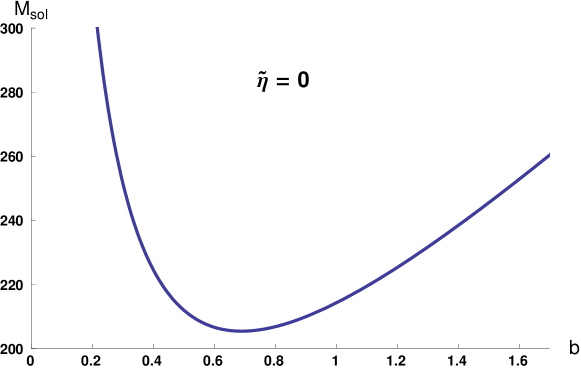
Figure 1: Soliton mass $M_{\text{sol}}$ in units $f/e$ vs. defect scale $b$ in units $1/(ef)$, for the case of $G_{N}=0$ and $f\neq 0$, corresponding to a vanishing coupling constant $\widetilde{\eta}\equiv 8\pi\,G_{N}\,f^{2}$.

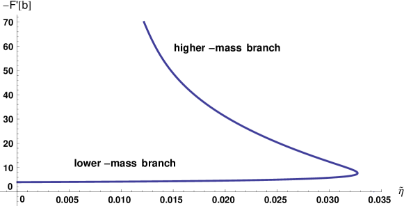
Figure 2: Two branches of the Skyrmion spacetime defect solution: matter-function slope $F^{\prime}(b^{2})$ vs. coupling constant $\widetilde{\eta}$, for defect scale $b=0.34/(ef)$ and metric-function boundary condition $\sigma(b^{2})=1$. At this value of $b$, the critical value of the coupling constant, $\widetilde{\eta}_{\text{crit}}$, is approximately equal to $0.033$.

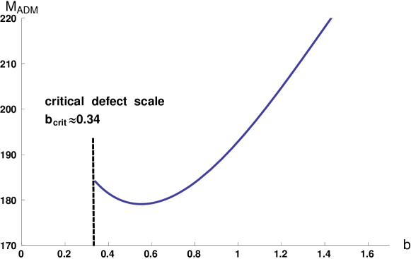
Figure 3: Gravitational mass $M_{\text{ADM}}$ in units $f/e$ vs. defect scale $b$ in units $1/(ef)$, for coupling constant $\widetilde{\eta}=0.033$ and boundary condition $\sigma(b^{2})=1$. These results correspond to the lower-mass branch of Fig. 2.

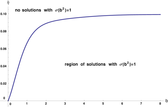
Figure 4: Curve of the critical defect scale $b_{\text{crit}}$ [in units of $1/(ef)$] and corresponding critical coupling constant $\widetilde{\eta}_{\text{crit}}$, where the boundary condition is fixed to $\sigma(b^{2})=1$. Above the curve, there are no globally regular solutions with $\sigma(b^{2})=1$.

From now on, we will refer to the coordinate-dependent quantity $M_{S}(W)$ from (19) as the “effective mass.” Therefore, the boundary condition $\sigma(b^{2})=1$ can be understood as having a vanishing effective mass at the defect surface. In this case, one expects that, for a given coupling constant $\widetilde{\eta}\neq 0$, the solution ceases to exist below some critical value of the defect scale. The numerical solution of the ODEs indeed shows this behavior (Fig. 3): starting from $b$ values near the minimum ADM mass, the soliton energy increases as $b$ decreases, but, at $b=b_{\text{crit}}$, the solution collapses, possibly even before an event horizon is formed. (The collapse of the gravitating $SU(2)$ Skyrmion has been discussed in, e.g., Ref. BizonChmaj1992 .) Note that, in the absence of gravity ($\widetilde{\eta}=0$), the collapse of the unit-winding-number $SO(3)$ Skyrmion is impossible and the soliton energy increases to infinity for $b\to 0^{+}$, as shown by Fig. 1.

With gravity present, the order of magnitude of $b_{\text{crit}}$ can be obtained from the following condition:

$$b=\kappa\;2\,G_{N}\,M_{\text{sol},\,\widetilde{\eta}=0}(b^{2})/c^{2}+\text{O}(\widetilde{\eta}^{2})\,,$$ (22)

where we have temporarily reinstated the light velocity $c$. In (22), $\kappa$ is a positive constant of order unity and $M_{\text{sol},\,\widetilde{\eta}=0}$ is given by the integral (16) for the case $\widetilde{\eta}=0$. The numerical results from Figs. 1 and 3 are consistent with (22) for $\kappa\approx 27/50$ : the first term on the right-hand side of (22) gives approximately $0.34/(ef)$ for $\widetilde{\eta}=0.033$ and $M_{\text{sol},\,\widetilde{\eta}=0}\approx 240\,f/e$ from the curve of Fig. 1 at $b=0.34/(ef)$, while the left-hand side of (22) corresponds to the direct numerical result $b_{\text{crit}}\approx 0.34/(ef)$ from Fig. 3. In Fig. 4, we show the numerical results for the dependence of $b_{\text{crit}}$ on the coupling $\widetilde{\eta}_{\text{crit}}$ at fixed boundary condition $\sigma(b^{2})=1$. Above the curve of Fig. 4, there are no globally regular solutions with $\sigma(b^{2})=1$ or $M_{S}(b^{2})=0$.

V Antigravity

Now, assume that the spacetime defects are remnants from some quantum-spacetime (QST) phase, as discussed in Sec. I. For simplicity, also assume that this phase determines a single characteristic scale of the defects, $b_{\text{QST}}>0$. There are two possibilities to consider. The first possibility is that the characteristic scale, for a fixed value of $\widetilde{\eta}$, corresponds to $b_{\text{QST}}^{\text{(1)}}\geq b_{\text{crit}}$ [lying, for example, in the $b>0.34/(ef)$ region of Fig. 3 ]. With the boundary condition $\sigma\big{(}b^{2}\big{)}=1$ for $b=b_{\text{QST}}^{\text{(1)}}$, the ADM mass is then always positive: the effective-mass function $M_{S}(W)$ is zero at $W=\big{(}b_{\text{QST}}^{\text{(1)}}\big{)}^{2}$ and increases monotonically with $W$.

The second possibility is that the characteristic scale, for a fixed value of $\widetilde{\eta}$, corresponds to

$$b_{\text{QST}}^{\text{(2)}}<b_{\text{crit}}\,,$$ (23)

where, from now on, the suffix “(2)” on the left-hand-side expression will be dropped and $b_{\text{crit}}$ on the right-hand side has been given explicitly in Fig. 4 and implicitly by (22). Then, in order to have globally regular solutions and to avoid gravitational collapse, we must have

$$0<\sigma(b^{2})\;\Big{|}_{b=b_{\text{QST}}}<1\,.$$ (24)

The condition (24) translates into $M_{S}(b_{\text{QST}}^{2})<0$, so that the effective mass at the defect surface is negative. Adding a sufficiently negative effective mass to the defect decreases the critical scale of the defect significantly, allowing for $b_{\text{QST}}\geq b_{\text{crit}}^{\text{(new)}}$. The effective-mass function $M_{S}(W)$ is still monotonic but starts from a negative value at $W=b^{2}$.

For finite values of $\widetilde{\eta}$, the ODEs (8) with nonstandard boundary condition $\sigma(b_{\text{QST}}^{2})<1$ from (24) [or $M_{S}(b_{\text{QST}}^{2})<0$] can be solved numerically and give an ADM mass (21) which can be negative, zero, or positive. Two numerical solutions are presented in Figs. 5 and 6 for parameters $\{\widetilde{\eta},\,b\}=\{1/10,\,1/(ef)\}$, which correspond to a point above the curve of Fig. 4. These numerical solutions have, depending on the value of the boundary condition $\sigma(b^{2})<1$, negative and positive ADM mass, as shown by the respective $l(w)$ panels in Figs. 5 and 6. The $\sigma(b^{2})$ dependence of the two-dimensional solution space, at three fixed values of $\widetilde{\eta}$, is given in Fig. 4.4 of Ref. Guenther2017 .

Figure 5: (Top row) Ansatz functions $F(w)$, $\sigma(w)$, and $\mu(w)$ of the numerical solution of the reduced field equations (8). The parameters are $\widetilde{\eta}\equiv 8\pi\,G_{N}\,f^{2}=1/10$ and $y_{0}\equiv efb=1$. The boundary conditions at the defect surface $w=(y_{0})^{2}=1$ are: $F=\pi$, $F^{\prime}=-0.323978148$, $\sigma=1/3$, and $\mu=2.21176$. (Middle row) Derived functions $w\,F(w)$, $l(w)\equiv\sqrt{w}\,\left[1-1/\sigma^{2}(w)\right]$, and $\sigma(w)\,\mu(w)$. (Bottom row) Dimensionless Ricci curvature scalar $R(w)$, dimensionless Kretschmann curvature scalar $K(w)$, and negative of the 00 component of the dimensionless Einstein tensor $E^{\mu}_{\;\;\nu}(w)$ $\equiv$ $R^{\mu}_{\;\;\nu}(w)-(1/2)\,R(w)\,\delta^{\mu}_{\;\;\nu}$, where the explicit expressions are given in App. B of Ref. Klinkhamer2014-prd .

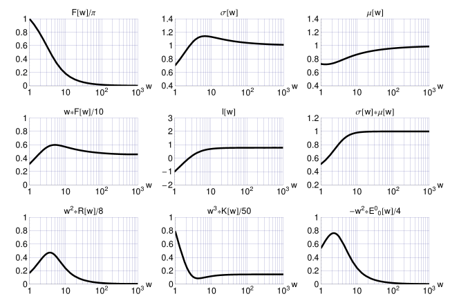
Figure 6: Same as Fig. 5, but now with the following boundary conditions at the defect surface $w=(y_{0})^{2}=1$: $F=\pi$, $F^{\prime}=-0.82561881304$, $\sigma=1/\sqrt{2}$, and $\mu=0.725818$.

Next, consider the special case $\widetilde{\eta}=0^{+}$, or explicitly

$$f^{2}\ll\big{(}E_{\text{planck}}\big{)}^{2}\equiv 1/(8\pi G_{N})\,,$$ (25)

and assume a small enough value of the remnant-defect scale (23). From the definition (20) and the ODE (11), there is then the following behavior: the value of $M_{S}(W)$ stays close to the negative value of $M_{S}(b_{\text{QST}}^{2})$ from (24) and the asymptotic ADM mass (21) is negative. For this special case, the negative ADM mass has been established by analytically solving ODE (11) for $\widetilde{\eta}=0$, with the trivial solution $l(w)=\text{const}=l(y_{0}^{2})$. But the $F(w)$ profile still requires the numerical solution of ODE (8c) with $\sigma^{2}(w)$ replaced by $\widetilde{\sigma}^{2}(w)\equiv 1/[1-l/\sqrt{w}\,]$ for constant $l\equiv l(y_{0}^{2})<0$, where $\widetilde{\sigma}(w)$ and $\widetilde{\mu}(w)=1/\widetilde{\sigma}(w)$ solve the ODEs (8a) and (8b) at $\widetilde{\eta}=0$. An explicit choice for $b_{\text{QST}}$ will be discussed in App. A, which also contains numerical results for the $F(w)$ profile. Additional numerical results are given in App. B.

Generally speaking, a negative ADM mass of the Skyrmion spacetime defect corresponds to a negative active gravitational mass (see, e.g., Ref. Bondi1957 for a discussion of negative masses in general relativity). The globally regular soliton then repels a distant test particle. Hence, there is “antigravity” from this particular Skyrmion spacetime defect, as long as the defect scale $b_{\text{QST}}$ and the coupling constant $\widetilde{\eta}$ are small enough.

VI Discussion

In this article, we have explained why a particular Skyrmion spacetime defect solution requires a negative ADM mass for its existence. In short, a nonstandard boundary condition on one of the metric functions is needed, $\sigma(b^{2})<1$, in order to avoid gravitational collapse and, for a small enough value of the coupling constant $\widetilde{\eta}\equiv 8\pi\,G_{N}\,f^{2}$, this boundary condition at the defect surface directly gives a negative ADM mass at spatial infinity. Whether or not such negative-gravitational-mass defects are present in the actual Universe depends on the nature of the quantum-spacetime phase and its supposed transition to an emerging classical spacetime. Needless to say, this quantum-spacetime phase is terra incognita.

Returning to the spacetime defect classical solution by itself, we have six general remarks on the physics of the negative-gravitational-mass soliton. First, the negative ADM mass found in Sec. V is not due to ponderable matter but to the gravitational fields at the defect surface $W=b^{2}$ (or $Y=0$). Indeed, the vacuum solution (18) with $R_{S}\equiv 2G_{N}M$ does not have a point where the curvature diverges and where ponderable matter can be thought to reside (the numerical value of constant $M$ is set by the gravitational fields themselves rather than by the ponderable matter). This behavior differs from that of the Schwarzschild solution [given by metric (12) with functions $\widehat{\mu}(r)=1/\widehat{\sigma}(r)=(1-2G_{N}\widehat{M}/r)$], which does have a point ($r=0$) where the curvature diverges and where ponderable matter can be thought to reside (this ponderable matter gives a positive numerical value for the constant $\widehat{M}$).

Second, the Skyrmion-spacetime-defect metric from (4) is degenerate: $\det g_{\mu\nu}=0$ at the defect surface $Y=0$, which corresponds to an $\mathbb{R}P^{2}$ submanifold. This degenerate metric makes that the singularity Gannon1975 and positive-mass SchoenYau1979 theorems are not directly applicable, allowing for a negative gravitational mass of the Skyrmion spacetime defect solution; see Sec. 3.1.5 of Ref. Guenther2017 for further discussion. The special feature of the Skyrmion spacetime defect solution is that certain geodesics at the defect surface $Y=0$ cannot be continued uniquely.

Third, the heuristic understanding of why there is degeneracy ($\det g_{\mu\nu}=0$) at the defect surface $Y=0$ is as follows. The two-dimensional defect surface at $Y=0$ corresponds to the projective plane $\mathbb{R}P^{2}$. Now, it is a well-known result that $\mathbb{R}P^{2}$ cannot be differentiably embedded in $\mathbb{R}^{3}$ (i.e., without intersections); cf. p. 40 in Ref. Nakahara1990 and Fig. 3 in Ref. Klinkhamer2014-mpla . For us, this result then suggests that the third extra dimension $Y$ emerging from the two-dimensional defect surface (local coordinates $X$ and $Z$) must have a vanishing metric component $g_{YY}$ at $Y=0$, which is precisely the structure of our metric Ansatz (4) for a finite value of $\sigma(b^{2})$. If the metric component $g_{YY}$ at $Y=0$ does not vanish, then there occur curvature singularities, as discussed in Sec. 5.2 of Ref. Schwarz2010 . Note that our defect-surface condition $\det g_{\mu\nu}=0$ is invariant under nonsingular coordinate transformations.

Fourth, having established that the Skyrmion spacetime defect has a negative active gravitational mass, as long as the defect scale $b$ and the coupling constant $\widetilde{\eta}$ are small enough, the question arises as to the value of its inertial mass. A positive inertial mass of the soliton-type solution would correspond to a dynamic violation of the equivalence principle, but this would not be altogether surprising as the solution is known to violate the standard elementary flatness property at the defect surface $Y=0$; see the paragraph under Eq. (2.29) in Ref. KlinkhamerSorba2014 for details.

Fifth, the negative-gravitational-mass Skyrmion spacetime defect may have other unusual properties, such as the nonstandard parity eigenvalues of scalar-field scattering solutions (a summary of the results appears in Sec. IV of Ref. KlinkhamerSorba2014 ).

Sixth, and finally, it remains to perform a rigorous stability analysis of the negative-gravitational-mass Skyrmion spacetime defect solution.

As to possible applications of antigravity by spacetime defects, two areas come to mind: cosmology (dark matter and dark energy) and condensed matter physics (analogue-gravity systems).

Appendix A Planck-scale defects

In Sec. V, we have given a general discussion of the antigravity effect coming from a small enough defect scale $b$, but we did not specify the actual size of the defect scale. In this appendix, we discuss a particular choice for the characteristic scale $b_{\text{QST}}$ of the defects, where the defects are considered to be remnants from an earlier quantum-spacetime (QST) phase.

First, restrict the matter sector of (3) to the following parameter domain:

$$f^{2} \ll \big{(}E_{\text{planck}}\big{)}^{2}\equiv 1/(8\pi G_{N})\approx\big{(}2.44\times 10^{18}\;\text{GeV}\big{)}^{2}\,,$$ (26a)

$$e \leq 1\,,$$ (26b)

where the first inequality corresponds to $\widetilde{\eta}\ll 1$ and where the origin of the upper bound on the coupling constant $e$ will be explained shortly. Next, assume that the characteristic scale of the defects is given by the Planck length,

$$b_{\text{QST}}=l_{\text{planck}}\equiv\sqrt{8\pi G_{N}\,\hbar/c^{3}}\approx 8.10\times 10^{-35}\;\text{m}\,,$$ (27)

which may very well be a typical scale of the quantum-spacetime phase (note the appearance of $\hbar$ in the square root of the above expression).

With the assumptions (26) and (27), condition (23) holds directly [in the terminology of the first two paragraphs of Sec. V, there is only the second possibility]. As explained in Sec. V, condition (23) implies that the globally regular solution must have $\sigma(b_{\text{QST}}^{2})<1$ and a corresponding negative ADM mass as given by (21). The reason is that, with $\widetilde{\eta}\ll 1$, the effective mass $M_{S}(W)$ is approximately constant for all $W$ values between $b^{2}$ and infinity. This behavior of nearly constant $M_{S}(W)$, or equivalently nearly constant $l(w)$ from (20), is already visible in Fig. 7 with numerical results for $\widetilde{\eta}=10^{-4}$, $e=1$, and defect scale $b=l_{\text{planck}}$ from (27). Observe also that the behavior of the bottom-row panels in Fig. 7 rapidly approaches the behavior of the defect vacuum solution (cf. Sec. 3 in Ref. Klinkhamer2014-mpla ) with vanishing Ricci curvature tensor, $R_{\mu\nu}^{\text{(vac)}}(w)=0$, and nonvanishing Kretschmann curvature scalar, $K^{\text{(vac)}}(w)\propto M^{2}/w^{3}$.

Let us now give the promised derivation of (26b). From Fig. 1 for $b\to 0^{+}$, we obtain $M_{\text{sol}}\propto 1/b$ or explicitly $M_{\text{sol}}\sim(70/y_{0})\,f/e$. With the latter result inserted in condition (22) for $b_{\text{crit}}$, condition (23) with $b=b_{\text{QST}}=l_{\text{planck}}$ translates into an upper bound on the matter coupling, $e<\sqrt{\kappa\,70/(4\pi)}\approx 1.73$ for $\kappa\approx 0.54$. In the bound (26b), we have just taken the number $1$ instead of the more accurate number $1.73$.

With the actual parameter value as stated in (26b), the difference between the defect scale $b$ from (27) and the critical scale $b_{\text{crit}}$ is a finite negative number, $b-b_{\text{crit}}<0$, and, therefore, requires a finite negative value for $\sigma(b^{2})-1$, in order to get a regular solution. In turn, a finite negative value of $\sigma(b^{2})-1$ corresponds to a finite negative value of $l(b^{2})$ as defined by (10), which implies, for $\widetilde{\eta}$ sufficiently close to $0$, a finite negative value of $\lim_{w\to\infty}l(w)$, i.e., a negative ADM mass, according to (20) and (21).

To summarize, for the matter theory (3) with restricted parameters (26), remnant spacetime defects with a length scale given by the Planck length (27) have a negative ADM mass, as long as they correspond to globally regular solutions. The implicit assumption, here, is that general relativity gives a more or less reliable description even for extremely small length scales as given by (27). But it is also possible that the defect scale is significantly larger than the Planck length, $b_{\text{QST}}=\zeta\,l_{\text{planck}}$ with a numerical factor $\zeta\gg 1$, provided the matter coupling constant is correspondingly reduced, $e\leq 1/\zeta\ll 1$.

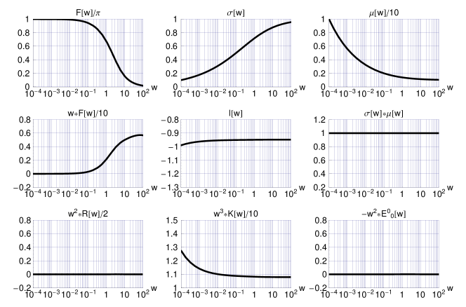
Figure 7: (Top row) Ansatz functions $F(w)$, $\sigma(w)$, and $\mu(w)$ of the numerical solution of the reduced field equations (8). The parameters are $\widetilde{\eta}\equiv 8\pi\,G_{N}\,f^{2}=10^{-4}$, $e=1$, and $y_{0}\equiv efb=efl_{\text{planck}}=10^{-2}$. The boundary conditions at the defect surface $w=(y_{0})^{2}=10^{-4}$ are: $F=\pi$, $F^{\prime}=-2.27604760$, $\sigma=1/10$, and $\mu=9.99298$. (Middle row) Derived functions $w\,F(w)$, $l(w)\equiv\sqrt{w}\,\left[1-1/\sigma^{2}(w)\right]$, and $\sigma(w)\,\mu(w)$. (Bottom row) Dimensionless Ricci curvature scalar $R(w)$, dimensionless Kretschmann curvature scalar $K(w)$, and negative of the 00 component of the dimensionless Einstein tensor $E^{\mu}_{\;\;\nu}(w)$ $\equiv$ $R^{\mu}_{\;\;\nu}(w)-(1/2)\,R(w)\,\delta^{\mu}_{\;\;\nu}$.

Appendix B Additional numerical results

The numerical results of Ref. Klinkhamer2014-prd are incorrect, because one of the three ODEs used contained some erroneous terms. As mentioned in Sec. II, the ODE (13a) in Ref. Klinkhamer2014-prd needs to be replaced by (8a). In this appendix, we present the corrected numerical results.

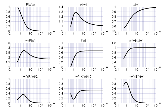
Figure 8: (Top row) Ansatz functions $F(w)$, $\sigma(w)$, and $\mu(w)$ of the numerical solution of the reduced field equations (8). The parameters are $\widetilde{\eta}=1/20$ and $y_{0}=1/\sqrt{2}$. The boundary conditions at the defect surface $w=(y_{0})^{2}=1/2$ are: $F=\pi$, $F^{\prime}=-1.9718377138$, $\sigma=1$, and $\mu=0.564337$. (Middle row) Derived functions $w\,F(w)$, $l(w)\equiv\sqrt{w}\,\left[1-1/\sigma^{2}(w)\right]$, and $\sigma(w)\,\mu(w)$. (Bottom row) Dimensionless Ricci curvature scalar $R(w)$, dimensionless Kretschmann curvature scalar $K(w)$, and negative of the 00 component of the dimensionless Einstein tensor $E^{\mu}_{\;\;\nu}(w)$ $\equiv$ $R^{\mu}_{\;\;\nu}(w)-(1/2)\,R(w)\,\delta^{\mu}_{\;\;\nu}$.

Figure 9: Core behavior of the functions from Fig. 9, in terms of the dimensionless quasiradial coordinate $y\in\mathbb{R}$. The coordinate $w$ is given by $w\equiv(y_{0})^{2}+y^{2}=1/2+y^{2}$.

Taking the parameter values $\{\widetilde{\eta},\,b\}=\{1/20,\,(1/\sqrt{2})/(ef)\}$, Fig. 9 replaces Figs. 2 and 3 of Ref. Klinkhamer2014-prd and Fig. 9 replaces Fig. 4 of Ref. Klinkhamer2014-prd . The boundary value $\sigma(b^{2})=1$ in Fig. 9 has been chosen to give approximately the same asymptotic $l$ value as in Fig. 3 of Ref. Klinkhamer2014-prd . Remark that the parameter values $\{\widetilde{\eta},\,b\}$ of Fig. 9 correspond to a point just below the curve of Fig. 4.

Figure 9 shows that the Ansatz functions of the numerical solution are perfectly smooth at the defect surface $Y=0$, as are the Ricci and Kretschmann curvature scalars and the energy density.

References

- (1) F.R. Klinkhamer, “Skyrmion spacetime defect,” Phys. Rev. D 90, 024007 (2014), arXiv:1402.7048.
-
(2)
F.R. Klinkhamer,
“Exotic physics: Antigravity?,”
talk at the workshop
Exotic Physics with Neutrino Telescopes 2013,
Marseille, 3–5 April 2013;
available from
https://indico.in2p3.fr/event/7381/contributions/41673/attachments/33518/41306/marseille_05apr2013.pdf -
(3)
M. Guenther,
“Skyrmion spacetime defect, degenerate metric,
and negative gravitational mass,”
Master Thesis, KIT, September 2017;
available from
https://www.itp.kit.edu/en/publications/diploma - (4) F.R. Klinkhamer, “A new type of nonsingular black-hole solution in general relativity,” Mod. Phys. Lett. A 29, 1430018 (2014), arXiv:1309.7011.
- (5) M. Schwarz, “Nontrivial spacetime topology, modified dispersion relations, and an -Skyrme model,” PhD Thesis, KIT, July 2010 (Verlag Dr. Hut, Munich, Germany, 2010; ISBN 9783868536232).
- (6) F.R. Klinkhamer and F. Sorba, “Comparison of spacetime defects which are homeomorphic but not diffeomorphic,” J. Math. Phys. 55, 112503 (2014), arXiv:1404.2901.
- (7) R. Arnowitt, S. Deser, and C.W. Misner, “Dynamical structure and definition of energy in general relativity,” Phys. Rev. 116, 1322 (1959).
- (8) A. Komar, “Positive-definite energy density and global consequences for general relativity,” Phys. Rev. 129, 1873 (1963).
- (9) P. Bizon and T. Chmaj, “Gravitating Skyrmions,” Phys. Lett. B 297, 55 (1992).
- (10) H. Bondi, “Negative mass in general relativity,” Rev. Mod. Phys. 29, 423 (1957).
- (11) D. Gannon, “Singularities in nonsimply connected spacetimes,” J. Math. Phys. 16, 2364 (1975).
- (12) R. Schoen and S.T. Yau, “On the proof of the positive mass conjecture in general relativity,” Commun. Math. Phys. 65, 45 (1979).
- (13) M. Nakahara, Geometry, Topology and Physics (IOP Publishing, Bristol, England, 1990).