A Provably Correct Algorithm for Deep Learning that Actually Works

Abstract

We describe a layer-by-layer algorithm for training deep convolutional networks, where each step involves gradient updates for a two layer network followed by a simple clustering algorithm. Our algorithm stems from a deep generative model that generates images level by level, where lower resolution images correspond to latent semantic classes. We analyze the convergence rate of our algorithm assuming that the data is indeed generated according to this model (as well as additional assumptions). While we do not pretend to claim that the assumptions are realistic for natural images, we do believe that they capture some true properties of real data. Furthermore, we show that our algorithm actually works in practice (on the CIFAR dataset), achieving results in the same ballpark as that of vanilla convolutional neural networks that are being trained by stochastic gradient descent. Finally, our proof techniques may be of independent interest.

1 Introduction

The success of deep convolutional neural networks (CNN) has sparked many works trying to understand their behavior. We can roughly separate these works into three categories: First, the majority of the works focus on providing various optimization methods and algorithms that prove well in practice, but have almost no theoretical guarantees. A second class of works focuses on analyzing practical algorithms (mostly SGD), but under strong assumptions on the data distribution, like linear separability or sampling from Gaussian distribution, that often make these problems trivially solvable by much simpler algorithms. A third class of works takes less restrictive assumptions on the data, provides strong theoretical guarantees, but these guarantees hold for algorithms that don’t really work in practice.

In this work, we study a new algorithm for learning deep convolutional networks, assuming the data is generated from some deep generative model. This model assumes that the examples are generated in a hierarchical manner: each example (image) is generated by first drawing a high-level semantic image, and iteratively refining the image, each time generating a lower-level image based on the higher-level semantics from the previous step. Similar models were suggested in other works as good descriptions of natural images encountered in real world data. These works, although providing important insights, suffer from one of two major shortcomings: they either suggest algorithms that seem promising for practical use, but without any theoretical guarantees, or otherwise provide algorithms with sound theoretical analysis that seem far from being applicable for learning real-world data.

Our work achieves promising results in the following sense: first, we show an algorithm along with a complete theoretical analysis, proving it’s convergence under the assumed generative model (as well as additional, admittedly strong, assumptions). Second, we show that implementing the algorithm to learn real-world data achieves performance that are in the same ballpark as the popular CNN trained with SGD-based optimizers. Third, the problem on which we apply our algorithm is not trivially learned by simple “shallow” learning algorithms. The main achievement of this paper is succeeding in all of these goals together. As is usually the case in tackling hard problems, our theoretical analysis makes strong assumptions on the data distribution, and we clearly state them in our analysis. Nevertheless, the resulting algorithm works on real data (where the assumptions clearly do not hold). That said, we do not wish to claim that such algorithm achieves state-of-the-art results, and hence did not apply many of the common “tricks” that are used in practice to train a CNN, but rather compared our algorithm to an “out-of-the-box” SGD-based optimization.

2 Related Work

As mentioned, we can roughly divide the works relevant to the scope of this paper into three categories: (1) works that study practical algorithms (SGD) solving “simple” problems that can be otherwise learned with “shallow” algorithms. (2) works that study problems with less restrictive assumptions, but using algorithms that are not applicable in practice. (3) works that study a generative model similar to ours, but either give no theoretical guarantees, or otherwise analyze an algorithm that is “tailored” to learning the generative model, and seems very far from algorithms used in practice.

Trying to study a practically useful algorithm, [5] proves that SGD learns a function that approximates the best function in the conjugate kernel space derived from the network architecture. Although this work provides guarantees for a wide range of deep architectures, there is no empirical evidence that the best function in the conjugate kernel space performs at the same ballpark as CNNs. The work of [1] shows guarantees on learning low-degree polynomials, which is again learnable via SVM or direct feature mapping. Other works study shallow (one-hidden-layer) networks under some significant assumptions. The works of [8, 4] study the convergence of SGD trained on linearly separable data, which could be learned with the Perceptron algorithm, and the works of [3, 15, 10, 20] assume that the data is generated from Gaussian distribution, an assumption that clearly does not hold in real-world data. The work of [6] extends the results in [3], showing recovery of convolutional kernels without assuming Gaussian distribution, but is still limited to the regime of shallow two-layer network.

Another line of work aims to analyze the learning of deep architectures, in cases that exceed the capacity of shallow learning. The works of [11, 18, 17] show polynomial-time algorithms aimed at learning deep models, but that seem far from performing well in practice. The work of [19] analyses a method of learning a model similar to CNN which can be applied to learn multi-layer networks, but the analysis is limited to shallow two-layer settings, when the formulated problem is convex.

Finally, there have been a few works suggesting distributional assumptions on the data that are similar in spirit to the generative model that we analyze in this paper. Again, these works can be largely categorized into two classes: works that provide algorithms with theoretical guarantees but no practical success, and works that show practical results without theoretical guarantees. The work of [2] shows a provably efficient algorithm for learning a deep representation, but this algorithm seems far from capturing the behavior of algorithms used in practice. Our approach can be seen as an extension of the work of [12], who studies Hierarchal Generative Models, focusing on algorithms and models that are applicable to biological data. [12] suggests that similar models may be used to define image refinement processes, and our work shows that this is indeed the case, while providing both theoretical proofs and empirical evidence to this claim. Finally, the works of [14, 13, 16] study generative models similar to ours, with promising empirical results when implementing EM inspired algorithms, but giving no theoretical foundations whatsoever.

3 Generative Model

We begin by introducing our generative model. This model is based on the assumption that the data is generated in a hierarchical manner. For each label, we first generate a high-level semantic representation, which is simply a small scale image, where each “pixel” represents a semantic class (in case of natural images, these classes could be: background, sky, grass etc.). From this semantic image, we generate a lower level image, where each patch comes from a distribution depending on each “pixel” of the high-level representation, generating a larger semantic image (lower level semantic classes for natural images could be: edges, corners, texture etc.). We can repeat this process iteratively any number of times, each time creating a larger image of lower level semantic classes. Finally, to generate a greyscale or RGB image, we assume that the last iteration of this process samples patches over $\mathbb{R}$. This model is described schematically in Figure 1, with a formal description given in Section 3.1. Section 3.2 describes a synthetic example of digit images generated according to this model.

3.1 Formal Description

To generate an example, we start with sampling the label $y\sim U(\mathcal{Y})$, where $U(\mathcal{Y})$ is the uniform distribution over the set of labels. Given $y$, we generate a small image with $m$ pixels, where each pixel belongs to a set $\mathcal{C}_{0}$. Elements of $\mathcal{C}_{0}$ corresponds to semantic entities (e.g. “sky”, “grass”, etc.). The generated image, denoted $x^{(0)}\in\mathcal{C}_{0}^{m}$, is sampled according to some simple distribution $\mathcal{D}_{y}$ (to be defined later). Next, we generate a new image, $x^{(1)}\in\mathcal{C}_{1}^{ms}$ as follows. Pixel $i$ in $x^{(0)}$ corresponds to some $c\in\mathcal{C}_{0}$. For every such $c$, there is a distribution $\mathcal{D}_{c}$ over $\mathcal{C}_{1}^{s}$, where we refer to $s$ as a “patch size”. So, pixel $i$ in $x^{(0)}$ whose value is $c\in\mathcal{C}_{0}$ generates a patch of size $s$ in $x^{(1)}$ by sampling the patch according to $\mathcal{D}_{c}$. This process continues, which yields images $x^{(2)},\ldots,x^{(k)}$ whose sizes are $ms^{2},\ldots,ms^{k}$, where each pixel in layer $i$ comes from $\mathcal{C}_{i}$. We assume that $\mathcal{C}_{k}=\mathbb{R}$, hence the final image is over the reals. The resulting example is the pair $(x^{(k)},y)$. We denote the distribution generating the image of level $i$ by $\mathcal{G}_{i}$.

Figure 1: Generative model schematic description

3.2 Synthetic Digits Example

To demonstrate our generative model, we use a small synthetic example to generate images of digits. In this case, we use a three levels model, where semantic classes represent lines, corners etc. In the notations above, we use:

$$\mathcal{C}_{0}=\{\includegraphics[scale={0.02}]{fig_sym0_0},\includegraphics[scale={0.02}]{fig_sym0_1},\includegraphics[scale={0.02}]{fig_sym0_2},\includegraphics[scale={0.02}]{fig_sym0_3},\includegraphics[scale={0.02}]{fig_sym0_4},\includegraphics[scale={0.02}]{fig_sym0_5},\includegraphics[scale={0.02}]{fig_sym0_6},\includegraphics[scale={0.02}]{fig_sym0_7},\includegraphics[scale={0.02}]{fig_sym0_8}\}~{}~{},~{}~{}\mathcal{C}_{1}=\{\includegraphics[scale={0.02}]{fig_sym1_0},\includegraphics[scale={0.02}]{fig_sym1_1},\includegraphics[scale={0.02}]{fig_sym1_2},\includegraphics[scale={0.02}]{fig_sym1_3},\includegraphics[scale={0.02}]{fig_sym1_4},\includegraphics[scale={0.02}]{fig_sym1_5}\}~{}~{},~{} \mathcal{C}_{2}=\mathbb{R}$$

We define the distributions $\mathcal{D}_{0},\dots,\mathcal{D}_{9}$ to be the distributions concentrated on the equivalent digital representation:  ,  ,  ,  ,  ,  ,  ,  ,  ,  .

Now, in the second level of the generative model, each pixel in $\mathcal{C}_{0}$ can generate one of four possible manifestations. For example, for the pixel , we sample over:  ,  ,  ,  . Similarly, in the final level we sample for each $c\in\mathcal{C}_{1}$ from a distribution $\mathcal{D}_{c}$ supported over 4 elements. For example, for the pixel , we sample over:  ,  ,  ,  .

Notice that though this example is extremely simplistic, it can generate $4^{9}$ examples per digit in the first level, and $4^{90}$ examples for each digit in the final layer, amounting to $9\cdot 4^{90}\approx 1.38\cdot 10^{55}$ different examples. Figure 2 shows the process output.

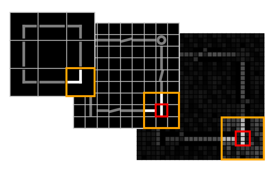
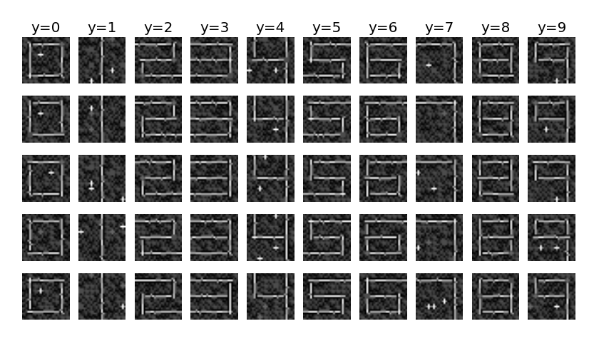
Figure 2: Left: Image generation process example. Right: Synthetic examples generated.

4 Algorithm

Assume we are given data from the generative distribution described in Section 3, our goal is to learn a classifier that predicts the label for each image. A natural approach would be to try to learn for each low-level patch, the semantic class (in the higher-level semantic image) from which it was generated. This way, we could cluster together semantically related patches, exposing the higher-level semantic image that generated the lower-level image. If we succeed in doing so multiple times, we can infer the topmost semantic image in the hierarchy. Assuming the high-level distribution $\mathcal{G}_{0}$ is simple enough (for example, a linearly separable distribution with respect to some embedding of the classes), we could then use a simple classification algorithm on the high-level image to infer its label.

Unfortunately, we cannot learn these semantic classes directly as we are not given access to the latent semantic images, but only to the lowest-level image generated by the model. To learn these classes, we use a combination of a simple clustering algorithm and a gradient-descent based algorithm that learns a single layer of a convolutional neural network. Surprisingly, as we show in the theoretical section, the gradient-descent finds an embedding of the patches such that patches from the same class are close to each other, while patches from different classes are far away. The clustering step then clusters together patches from the same class.

4.1 Algorithm Description

The algorithm we suggest is built from three building-blocks composed together to construct the full algorithm: (1) clustering algorithm, (2) gradient-based optimization of two-layer Conv net and (3) a simple classification algorithm. In order to expose the latent representation of each layer in the generative model, we perform the following iteratively:
(1) Run a centroid-based clustering algorithm on the patches of size $\sqrt{s}\times\sqrt{s}$ from the input image defined by the previous step (or the original image in the first step), w.r.t. the cosine distance, to get $\ell$ cluster centers.
(2) Run a convolution operation with the cluster centroids as kernels, followed by ReLU with a fixed bias and a pooling operation. This will result in mapping the patches in the input images to (approximately) orthogonal vectors in an intermediate space $\mathbb{R}^{\ell}$.
(3) Initialize a 1x1 convolution operation, that maps from $\ell$ channels into $n$ channels, followed by a linear layer that will output $|\mathcal{Y}|$ channels (where it’s input is the $n\times m\times m$ tensor flattened into a vector). We train this two-layer subnet using a gradient-based optimization method. As we show in the analysis, this step implicitly learns an embedding of the patches into a space where patches from the same semantic class are close to each other, while patches from different classes are far away, hence laying the ground for the clustering step of the next iteration.
(4) “Throw” the last linear layer, thus leaving a trained block of Conv$(\sqrt{s}\times\sqrt{s})$-ReLU-Pool-Conv$(1\times 1)$ which finds a “good” embedding of the patches of the input image, and repeat the process again, where the output of this block is the input to step 1.

Finally, after we perform this process for $k$ times, we get a network of depth $k$ composed from Conv$(\sqrt{s}\times\sqrt{s})$-ReLU-Pool-Conv$(1\times 1)$ blocks. Then, we feed the output of this (already trained) network to some classifier, training it to infer the label $y$ from the semantic representation that the convolution network outputs. This training is done again using a gradient-based optimization algorithm. We now describe the building blocks for the algorithm, followed by the definition of the complete algorithm.

4.1.1 Clustering

The first block of the algorithm is the clustering step. We denote $\textrm{CLUSTER}_{\gamma}$ to be any polynomial time clustering algorithm, such that given a sample $S\subseteq\mathbb{R}^{s}$, the algorithm outputs a mapping $\phi_{S}:\mathbb{R}^{s}\rightarrow\mathbb{R}^{\ell}$, satisfying that for every $x_{i},x_{j}\in S$, if $\|x_{i}-x_{j}\|<\gamma$ then $\phi_{S}(x_{i})=\phi_{S}(x_{j})$, and if $\|x_{i}-x_{j}\|>2\gamma$ then $\phi_{S}(x_{i})\perp\phi_{S}(x_{j})$. Notice that this clustering could be a trivial clustering algorithm: for each example, we cluster together all the examples that are within $\gamma$ distance from it, mapping different clusters to orthogonal vectors in $\mathbb{R}^{\ell}$. Thus, we take $\ell$ to be the number of clusters found in $S$.

For the consistency with common CNN architecture, we can use a centroid-based clustering algorithm that outputs the centroid of each cluster, using these cetnroids as kernels for a convolution operation. Combining this with ReLU with a fixed bias and a pooling operation gives an operation that maps each patch to a single vector, where vectors of different patches are approximately orthogonal.

4.1.2 Two-Layer Network Algorithm

The second building-block of our main algorithm is a gradient-based optimization algorithm that is used to train a two-layer convolutional subnet. In this paper, we define a convolutional subnet to be a function $\mathcal{N}_{K,W}:\mathbb{R}^{\ell\times m}\rightarrow\mathbb{R}$ defined by:

$$\mathcal{N}_{K,W}(X)=\langle W^{\top},K^{\top}X\rangle$$

Where we define the inner product between matrices $A,B$ as $\langle A,B\rangle:=\mathrm{tr}(AB)$.

This is equivalent to a convolution operation on an image, followed by a linear weighted sum: assume $X$ is the matrix where each column is a patch in an image (the “im2col” operation), then multiplying this matrix by $K^{\top}$ is equivalent to performing a convolution operation with kernels $\bm{k}^{(1)},\dots,\bm{k}^{(n)}$ on the original image (where we denote $\bm{k}^{(i)}$ to be the $i$-th vector of matrix $K$). Flattening the resulting matrix and multiplying by the weights in $W$ yields the second linear layer.

The top linear layer of the network outputs a prediction for the label $y\in\mathcal{Y}$, and is trained with respect to the loss $\mathcal{L}_{K,W}^{S}$ on a given set of examples $S$, defined as:

$$\mathcal{L}^{S}_{K,W}=\mathbb{E}_{(X,y)\sim S}\left[\ell_{y}(\mathcal{N}_{K,W}(X))\right]$$

For some loss function $\ell:\mathbb{R}\times\mathcal{Y}\rightarrow\mathbb{R}$.

After removing the top linear layer (which is used only to train the convolutional layer), this algorithm will output the matrix $K$. This matrix is a set of 1x1 convolution kernels learned during the optimization, that are used on top of the previous operations. We denote $\mathrm{TLGD}(S,T,\eta,n,\sigma)$ the algorithm that trains a two-layer network of width $n$, on sample $S$ for $T$ iterations with learning rate $\eta$, randomly initializing $K,W$ from some distribution with parameter $\sigma$ (described in details in the theoretical section). This algorithm outputs the Conv1x1 kernels learned.

As we show in our theoretical analysis, running a gradient-based algorithm will implicitly learn an embedding that maps patches from the same class to similar vectors, and patches from different classes to vectors that are far away.

4.1.3 Classification Algorithm

Finally, the last building block of the algorithm is a classification stage, that is used on top of the deep convolution architecture learned in the previous steps. We consider some hypothesis space $\mathcal{H}\subset\mathcal{Y}^{\mathcal{X}}$ (for example linear separators). Denote CLS a polynomial time classification algorithm, such that given a sample $S\subseteq\mathcal{X}\times\mathcal{Y}$, the algorithm outputs some hypothesis $\textrm{CLS}(S)\in\mathcal{H}$. Again, we can assume this algorithm is trained using a gradient-based optimization algorithm, to infer the label $y\in\mathcal{Y}$ based on the high-level semantics generated by the deep convolutional network trained in the previous steps.

4.1.4 Complete Algorithm

Utilizing the building blocks described previously, our algorithm learns a deep CNN layer after layer. This network is used to infer the label for each image. This algorithm is described formally in Algorithm 1. In the description, we use the notation $\phi\ast A$ to denote the operation of applying a map $\phi:\mathcal{K}_{0}^{m_{0}}\rightarrow\mathcal{K}_{1}^{m_{1}}$ on a tensor $A$, replacing patches of size $m_{0}$ by vectors in $\mathcal{K}_{1}^{m_{1}}$. Formally:

$$\phi\ast A:=[\phi(A_{:,i\cdot m_{0}\dots(i+1)\cdot m_{0}})]_{i}$$

Algorithm 1 Deep Layerwise Clustering

  input:

     numbers $\gamma,\eta,T,n,\sigma$

     sample $S=\{(x_{1},y_{1}),\dots(x_{N},y_{N})\}\subseteq\mathbb{R}^{ms^{k}}\times\mathcal{Y}$

  $h_{k}\leftarrow id$

  for $\kappa=k\dots 1$ do

     // construct sample of examples after running through the current network

     set $S_{\kappa}\leftarrow\{(h_{\kappa}(x_{1}),y_{1}),\dots,(h_{\kappa}(x_{N}),y_{N})\}$

     // generate patches from the current sample, and cluster together

     set $P_{\kappa}\leftarrow\{\mathrm{patches~{}of~{}size~{}\sqrt{s}\times\sqrt{s}~{}from~{}}S_{\kappa}\}$

     set $\phi_{\kappa}\leftarrow\textrm{CLUSTER}_{\gamma}(P_{\kappa})$

     // map the patches into orthogonal vectors using the embedding $\phi_{\kappa}$

     set $\hat{S}_{\kappa}\leftarrow\{(\phi_{\kappa}\ast h_{\kappa}(x_{1}),y_{1}),\dots,(\phi_{\kappa}\ast h_{\kappa}(x_{N}),y_{N})\}$

     // train a two-layer network to find a “good” embedding for the patches

     set $K_{\kappa-1}\leftarrow\textrm{TLGD}(\hat{S}_{\kappa},T,\eta,n,\sigma)$

     // add the current block to the network

     set $h_{\kappa-1}\leftarrow K_{\kappa-1}^{\top}(\phi_{\kappa}\ast h_{\kappa})$

  end for

  // run a final clustering on the vectors of the current sample

  set $S_{0}\leftarrow\{(h_{0}(x_{1}),y_{1}),\dots,(h_{0}(x_{N}),y_{N})\}$

  set $P_{0}\leftarrow\{\mathrm{patches~{}of~{}size~{}1\times 1~{}from~{}}S_{0}\}$

  set $\phi_{0}\leftarrow\textrm{CLUSTER}_{\gamma}(P_{k})$

  // train the final classifier to predict the labels from the CNN output

  set $\hat{S}_{0}\leftarrow\{(\phi_{0}\ast h_{0}(x_{1}),y_{1}),\dots,(\phi_{0}\ast h_{0}(x_{N}),y_{N})\}$

  set $h\leftarrow\textrm{CLS}(\hat{S}_{0})$

  return $h\circ h_{0}$

5 Theoretical Analysis

In this section we prove that, under some assumptions, the algorithm described in Algorithm 1 learns (with high probability) a network model that correctly classifies the examples according to their labels. The structure of this section is as follows. We first introduce our assumptions on the data distribution as well as on the specific implementation of the algorithm. Next, we turn to the analysis of the algorithm itself, starting with showing that the sub module of training a two-layer network implicitly learns an embedding of the patches into a space where patches from a similar semantic class are close to each other, while patches from different classes are far apart. Using this property, we show that even a trivial clustering algorithm manages to correctly cluster the patches. Finally, we prove that performing these two steps (two-layer network + trivial clustering) iteratively, layer by layer, leads to revealing the underlying model.

5.1 Assumptions

Our analysis relies on several assumptions on the data distribution, as well as on the suggested implementation of the algorithm. These assumptions are necessary for the theorems to hold, and admittedly are far from being trivial. We believe that some of the assumptions can be relaxed on the expense of a much more complicated proof.

5.1.1 Distributional Assumptions

For simplicity, we focus on binary classification problems, namely, $\mathcal{Y}=\{\pm 1\}$. The extension to multi-class problems is straightforward. We assume that the sets of semantic classes $\mathcal{C}_{0},\dots,\mathcal{C}_{k-1}$ are finite, and the final (observed) image is over the reals, i.e $\mathcal{C}_{k}=\mathbb{R}$.

We assume the following is true for all $\kappa\in[k]$. For all $c\in\mathcal{C}_{\kappa}$ the distribution of the patches in the lower-level image for pixels of value $c$, denoted $\mathcal{D}_{c}$, is a uniform distribution over a finite set of patches $S_{c,\kappa}\subseteq\mathcal{C}_{\kappa+1}^{s}$. We further assume that all these sets are disjoint and are of fixed size $d$.

For every $c$ we denote by $\mathcal{F}_{c}$ the operator that takes a tensor (of some dimension) as its input and replaces every element of the input by the boolean that indicates whether it equals to $c$.

We introduce the notation: $v^{\kappa}_{c}:=\mathbb{E}_{(z,y)\sim\mathcal{G}_{\kappa}}\left[-y\mathcal{F}_{c}(z)\right]\in\mathbb{R}^{ms^{\kappa}}$.

Notice that $-v^{\kappa}_{c}$ is the “mean” image over the distribution for every given semantic class, $c$. For example, semantic classes that tend to appear in the upper-left corner of the image for positive images will have positive values in the upper-left entries of $-v_{c}^{\kappa}$. As will be explained later, these images play a key role in our analysis.

For our analysis to follow, we assume that the vectors $\{v_{c}^{\kappa}\}_{c\in\mathcal{C}_{\kappa}}$ are linearly independent. For each $c_{1},c_{2}\in\mathcal{C}_{\kappa}$ we denote the angle between $v^{\kappa}_{c_{1}}$ and $v^{\kappa}_{c_{2}}$ by:

$$\angle(v^{\kappa}_{c_{1}},v^{\kappa}_{c_{2}}):=\arccos\left(\frac{v^{\kappa}_{c_{1}}\cdot v^{\kappa}_{c_{2}}}{\|v^{\kappa}_{c_{1}}\|\|v^{\kappa}_{c_{2}}\|}\right)\in[0,\pi]$$

Denote $\theta:=\min_{\kappa<k,c_{1},c_{2}\in\mathcal{C}_{\kappa}}\angle(v^{\kappa}_{c_{1}},v^{\kappa}_{c_{2}})$ and $\lambda:=\min_{\kappa<k,c\in\mathcal{C}_{\kappa}}\|v^{\kappa}_{c}\|$. From the linear independence assumption it follows that both $\theta$ and $\lambda$ are strictly positive. The convergence of the algorithm depends on $1/\theta$ and $1/\lambda$.

5.1.2 High Level Efficient Learnability

The essence of the problem to learn the mapping from the images in $R^{ms^{k}}$ to the labels is that we do not observe the high level semantic image in $\mathcal{C}_{0}^{m}$. To make this distinction clear, we assume that, had we were given the semantic images in $\mathcal{C}_{0}^{m}$, then the learning problem would have been easy. Formally, there exists a classification algorithm, denoted CLS, that upon receiving an i.i.d. training set of polynomial size from the distribution $\mathcal{G}_{0}$ over $\mathcal{C}_{0}^{m}\times\{\pm 1\}$, it returns (with high probability, and after running in polynomial time) a classifier whose error is at most $\epsilon$.

5.1.3 Assumptions on the Implementation of the Two Layers Building Block

For the analysis, we train the two-layer network with respect to the loss $\ell_{y}(\hat{y})=-y\hat{y}$. This loss simplifies the analysis, and seems to capture a similar behavior to other loss types used in practice.

Although in practice we perform a variant of SGD on a sample of the data to train the network, we perform the analysis with respect to the population loss: $\mathcal{L}_{K,W}=\mathbb{E}_{(X,y)\sim\mathcal{G}}\left[\ell_{y}(\mathcal{N}_{K,W}(X))\right]$. We denote $K_{t}\in\mathbb{R}^{\ell\times n}$ the weights of the first layer of the network in iteration $t$, and denote $W_{0}\in\mathbb{R}^{n\times m}$ the initial weights of the second layer. For simplicity of the analysis, we assume that only the first layer of the network is trained, while the weights of the second layer are fixed. Thus, we perform the following update step at each iteration of the gradient descent: $K_{t}=K_{t-1}-\eta\frac{\partial}{\partial K}\mathcal{L}_{K_{t-1},W_{0}}$. Applying this multiple times trains a network, denoted $\mathcal{N}_{K_{t},W_{0}}$.

As for the initialization of $K_{0},W_{0}$, assume we initialize each column of $K_{0}$ from a uniform distribution on a sphere whose radius is at most $\frac{\sigma}{2\sqrt{n}}$, where $\sigma$ is a parameter of the algorithm and $n$ is the number of columns of $K_{0}$. We initialize $W_{0}\sim\mathcal{N}(0,1)$.

5.2 Two-Layer Algorithm

In this part of the analysis we limit ourselves to observing the properties of the two-layer network trained in the $\kappa$ iteration of the main algorithm. Hence, we introduce a few simple notations to make the analysis clearer. We first assume that we are given some mapping from patches to $\mathbb{R}^{\ell}$, denoted $\phi:\mathcal{C}_{\kappa}^{s}\rightarrow\mathbb{R}^{\ell}$, such that $\mathrm{Im}(\phi)$ is a set of orthonormal vectors (this mapping is learned by the previous steps of the algorithm, as we show in Section 5.3). Assume we observe the distribution $\mathcal{G}:=\phi\ast\mathcal{G}_{\kappa}$. Recall that $\mathcal{G}_{\kappa}$ is generated from the latent distribution $\mathcal{G}_{\kappa-1}$ over higher level images. We overload the notation and use $m$ to denote the size of the semantic images from the higher level of the model (namely, $m:=ms^{\kappa-1}$). Thus, $\mathcal{G}$ is a distribution over $\mathbb{R}^{\ell\times m}\times\{\pm 1\}$.

Now, we can “forget” the intermediate latent distributions $\mathcal{G}_{0},\dots,\mathcal{G}_{\kappa-2}$, and assume the distribution $\mathcal{G}_{\kappa-1}$ is given by sampling $y\sim U(\{\pm 1\})$ and then by sampling $(z,y)\sim\mathcal{D}_{y}$, where $z\in\mathcal{C}_{\kappa-1}^{m}$ and we use $\mathcal{D}_{y}$ to denote the distribution $\mathcal{G}_{\kappa-1}$ conditioned on $y$. Finally, we denote $\mathcal{G}_{z}$ the distribution $\mathcal{G}$ conditioned on $z$. Thus, we can describe the sampling from $\mathcal{G}$ schematically by:

$$\rightsquigarrow^{U(\mathcal{Y})}y\rightsquigarrow^{\mathcal{D}_{y}}(z,y)\rightsquigarrow^{\mathcal{G}_{z}}(X,y)\in\mathbb{R}^{\ell\times m}\times\{\pm 1\}$$

We denote $\mathcal{C}:=\mathcal{C}_{\kappa-1}$, which is the set of the semantic classes of the images in the latent distribution $\mathcal{G}_{\kappa-1}$. For every $c\in\mathcal{C}$ denote $S_{c}:=\{\phi(p)\}_{p\in S_{c,\kappa-1}}$, which is the application of $\phi$ on the set of patches in the observed distribution generated from the semantic class $c$. Notice that from the assumption on $\phi$ it follows that $\cup_{c\in\mathcal{C}}S_{c}$ is a set of orthonormal vectors. Denote $v_{c}=v^{\kappa-1}_{c}$, the “mean” image of the semantic class $c$. The following diagram describes the process of generating $X$ from $z$, with $\tilde{x}$ being the example generated by distribution $\mathcal{G}_{\kappa}$ (the example which is embedded into the observed space $\mathbb{R}^{\ell\times m}$):

$$\tiny\underbrace{\left[\begin{matrix}z_{1}\\ \vdots\\ z_{m}\end{matrix}\right]}_{z\in\mathcal{C}^{m}}\rightsquigarrow\underbrace{\left[\begin{matrix}\tilde{x}_{1}\\ \vdots\\ \tilde{x}_{s}\\ \vdots\\ \tilde{x}_{ms-s+1}\\ \vdots\\ \tilde{x}_{ms}\end{matrix}\right]}_{\tilde{x}\in\mathcal{C}_{\kappa}^{ms}}\overset{\mathrm{im2col}}{\mapsto}\left[\begin{matrix}\tilde{x}_{1}&\dots&\tilde{x}_{ms-s+1}\\ \vdots&&\vdots\\ \tilde{x}_{s}&\dots&\tilde{x}_{ms}\\ \end{matrix}\right]\overset{\phi}{\mapsto}\underbrace{\left[\begin{matrix}\overbrace{\phi\left(\begin{matrix}\tilde{x}_{1}\\ \vdots\\ \tilde{x}_{s}\end{matrix}\right)}^{\bm{x}^{(1)}\in S_{z_{1}}}&\dots&\overbrace{\phi\left(\begin{matrix}\tilde{x}_{ms-s+1}\\ \vdots\\ \tilde{x}_{ms}\end{matrix}\right)}^{\bm{x}^{(m)}\in S_{z_{m}}}\end{matrix}\right]}_{X\in\mathbb{R}^{\ell\times m}}$$

Now, we can introduce the main theorem of this section. This theorem states that training the two-layer Conv net as defined previously will implicitly learn an embedding of the observed patches into a space such that patches from the same semantic class are close to each other, while patches from different classes are far. Recall that we do not have access to the latent distribution, and thus cannot possibly learn such embedding directly. Therefore, this surprising property of gradient descent is the key feature that allows our main algorithm to learn the high-level semantics of the images.

Theorem 1

Let $\theta,\lambda$ be as described in Section 5.1.1. Assume we train a two-layer network of size $n>\frac{2\pi}{0.23\theta}\log(\frac{|\mathcal{C}|}{\delta})$ with respect to the population loss on distribution $\mathcal{G}$, with learning rate $\eta$, for $T>\frac{2\sqrt{s}\sigma d}{\eta\lambda}$ iterations. Assume that the training is as described in Section 5.1.3, where the parameter $\sigma$ of the initialization is also described there. Then with probability of at least $1-\delta$:

1. for each $c\in\mathcal{C}$, for every $x_{1},x_{2}\in S_{c}$ we get $\|K_{T}^{\top}\cdot x_{1}-K_{T}^{\top}\cdot x_{2}\|<\sigma$

2. for $c_{1},c_{2}\in\mathcal{C}$, if $c_{1}\neq c_{2}$, for every $x_{1}\in S_{c_{1}},x_{2}\in S_{c_{2}}$, we get $\|K_{T}^{\top}\cdot x_{1}-K_{T}^{\top}\cdot x_{2}\|>2\sqrt{s}\sigma$

For lack of space, we give the full proof of this theorem in the appendix, and give a rough sketch of the proof here: Observe the value of $\bm{k}^{(i)}_{t}\cdot x^{\prime}$, which is the activation of a kernel in the first layer, denoted $\bm{k}^{(i)}_{t}$, operated on a given patch $x^{\prime}\in S_{c}$. Due to the gradient descent update rule, this value changes by $-\eta x^{\prime}\cdot\frac{\partial}{\partial\bm{k}^{(i)}}\mathcal{L}_{K_{t},W_{0}}$ at each iteration. Analyzing this gradient shows that this expression, i.e the change in the activation $\bm{k}^{(i)}_{t}\cdot x^{\prime}$, is in fact proportional to $\bm{w}^{(i)}_{0}\cdot v_{c}$. In other words, the value of $\bm{w}^{(i)}_{0}\cdot v_{c}$ is the only factor that dominates the behavior of the gradient with respect to $\bm{k}^{(i)}$. Hence, the activation of two patches generated from the same class will behave similarly throughout the training process. Furthermore, for patches from different classes $c_{1}\neq c_{2}$, if we happen to get: $\operatorname{sign}\left(\bm{w}^{(i)}_{0}\cdot v_{c_{1}}\right)\neq\operatorname{sign}\left(\bm{w}^{(i)}_{0}\cdot v_{c_{1}}\right)$, due to the random initialization (which will happen in sufficient probability), then the activations of patches from class $c_{1}$ and patches from class $c_{2}$ will go in opposite directions, and after enough iterations will be far apart.

To give more intuition as to why the proof works, we can look at the whole process from a different angle. For two patches in an image sampled from a given distribution, we can look at two measures of similarity: First, we can observe a simple “geometric” similarity, like the $\ell_{2}$ distance between these two patches. Second, we can define a “semantic” similarity between patches to be the similarity between the distribution of occurrences of each patch across the image (i.e, patches that tend to appear more in the upper part of the image for positive labels are in this sense “semantically” similar). In our case, we show that the vector $v_{c}$ gives us exactly this measure of similarity: two patches from the same class are semantically similar in the sense that their mean distribution in the image is exactly the same image, denoted $v_{c}$. Given this notion, we can see why our full algorithm works: the clustering part of the algorithm merges together geometrically similar patches, while the gradient descent algorithm maps semantically similar patches to geometrically similar vectors, allowing the clustering of the next iteration to perform clustering based again on the simple geometrical distance. Note that while the technical proof heavily relies on our assumptions, the intuitions above may hold true for real data.

5.3 Full Network Training

In this section, we analyze the convergence of the full algorithm described in Algorithm 1, where our main claim is that this algorithm successfully learns a model that classifies the examples sampled from the observed distribution $\mathcal{G}_{k}$. Formally, our main claim is given in the following theorem:

Theorem 2

Suppose that the assumptions given in Section 5.1 hold. Fix $\epsilon,\delta\in(0,\frac{1}{4})$, and let $\delta^{\prime}=\frac{\delta}{k+1}$. Denote $C:=\max_{\kappa<k}|\mathcal{C}_{\kappa}|$ the maximal number of semantic classes in each level $\kappa$. Let $\Delta$ denote the minimal distance between any two possible different patches in the observed images in $\mathbb{R}^{ms^{k}}$. Choose $\gamma\leq\frac{1}{2}\Delta$, $\sigma=\frac{\gamma}{\sqrt{s}}$, $n>\frac{2\pi}{0.23\theta}\log(\frac{C}{\delta})$, $T>\frac{2\sqrt{s}\sigma d}{\eta\lambda}$. Then, with probability $1-\delta$, running Algorithm 1 with parameters $\epsilon,\gamma,\eta,T,n,\sigma$ on data from distribution $\mathcal{G}_{k}$ returns hypothesis $h$ such that $P_{(x,y)\sim\mathcal{G}_{k}}(h(x)\neq y)<\epsilon$.

To show this, we rely on the result of Section 5.2, which guaranties that the embedding learned by the network at each iteration maps patches from the same class to similar vectors. Now, recall that our model assumes that a single pixel in a high-level image is “manifested” as a patch in the lower-level image. Thus, a patch of size $s$ in the higher-level image is manifested in $s^{2}$ patch in the lower-level image, and many such manifestations are possible. Thus, the fact that we find such “good” embedding allows our simple clustering algorithm to cluster together different low-level manifestations of a single high-level patch. Hence, iteratively applying this embedding and clustering steps allows to decode the topmost semantic image, which can be then classified by our simple classification algorithm.

Before we show the proof, we remind a few notations that were used in the algorithm’s description. We use $\phi_{\kappa}$ to denote the clustering of patches learned in the $\kappa$ iteration of the algorithm, and $K_{\kappa}$ the weights of the kernels learned BEFORE the $\kappa$ step (thus, the patches mapped by $K_{\kappa}$ are the input to the clustering algorithm that outputs $\phi_{\kappa}$). Note that in every step of the algorithm we perform a clustering on patches of size $s$ in the current latent image, while at the last step we cluster only patches of size $1$ (i.e, cluster the vectors in the “channels” dimension). This is because after the final iteration we have a mapping of the distribution $\mathcal{G}_{1}$, where patches of the same class are mapped to similar vectors. To generate a mapping of $\mathcal{G}_{0}$, we thus only need to cluster these vectors together, to get orthonormal representations of each class. Finally, we use the notations $\phi\ast A$ to indicate that we operate $\phi$ on every patch of the tensor $A$. When we use operations on distributions, for example $h\circ\mathcal{G}$ or $\phi\ast\mathcal{G}$, we refer to the new distribution generated by applying these operation to every examples sampled from $\mathcal{G}$. The essence of the proof is the following lemma:

Lemma 1

Let $\mathcal{G}:=\mathcal{G}_{k}$ be the distribution over pairs $(x,y)$, where $x$ is the observed image over the reals, and recall that for $\kappa<k$, the distribution $\mathcal{G}_{\kappa}$ is over pairs $(x,y)$ where $x$ is in a space of latent semantic images over $\mathcal{C}_{\kappa}$. For every $\kappa\in[k]$, with probability at least $1-\kappa\delta^{\prime}$, there exists an orthonormal patch mapping $\varphi_{\kappa}:\mathcal{C}_{\kappa}^{s}\rightarrow\mathbb{R}^{\ell}$ such that $\phi_{\kappa}\ast(h_{\kappa}\circ\mathcal{G})=\varphi_{\kappa}\ast\mathcal{G}_{\kappa}$, where $\phi_{\kappa}$ and $h_{\kappa}$ are as defined in Algorithm 1.

The proofs of the lemma and of Theorem 2 are given in Appendix B. The lemma tells us that the neural network at step $\kappa$ of the algorithm reveals (in some sense) the latent semantic structure.

6 Experiments

As mentioned before, our analysis relies on distributional assumptions formalized in the generative model we suggest. A disadvantage of such analyses is that the assumptions rarely hold for real-world data, as the distribution of natural images is far more complex. The goal of this section is to show that when running our algorithm on CIFAR-10, the performance of our model is in the same ballpark as a vanilla CNN, trained with a common SGD-based optimization algorithm. Hence, even though the data distribution deviates from our assumptions, our algorithm still achieves good performance.

We chose the CIFAR-10 problem, as a rich enough dataset of natural images. As our aim is to show that our algorithm achieves comparable result to a vanilla SGD-based optimization, and not to achieve state-of-the-art results on CIFAR-10, we do not use any of the common “tricks” that are widely used when training deep networks (such as data augmentation, dropout, batch normalization, scheduled learning rate, averaging of weights across iterations etc.). We implemented our algorithm by repeating the following steps twice: (1) Sample $N$ patches of size 3x3 uniformly from the dataset. (2) For some $\ell$, run the K-means algorithm to find $\ell$ cluster centers $c_{1}\dots c_{\ell}$. (3) At this step, we need to associate each cluster with a vector in $\mathbb{R}^{\ell}$, such that the image of this mapping is a set of orthonormal vectors, and then map every patch in every image to the vector corresponding to the cluster it belongs to. We do so by performing Conv3x3 layer with the $\ell$ kernels $c_{1}\dots c_{\ell}$, and then perform ReLU operation with a fixed bias $b$. This roughly maps each patch to the vector $e_{i}$, where $i$ is the cluster the patch belongs to. (4) While our analysis corresponds to performing the convolution from the previous step with a stride of $3$, to make the architecture closer to the commonly used CNNs (specifically the one suggested in the Tensorflow implementation [7]), we used a stride of $1$ followed by a 2x2 max-pooling. (5) Randomly initialize a two layered linear network, where the first layer is Conv1x1 with $\ell^{\prime}$ output channels, and the second layer is a fully-connected Affine layer that outputs 10 channels to predict the 10 classes of CIFAR-10. (6) Train the two-layers with Adam optimization ([9]) on the cross-entropy loss, and remove the top layer. The output of the first layer is the output of these steps.

Repeating the above steps twice yields a network with two blocks of Conv3x3-ReLU-Pool-Conv1x1. We feed the output of these steps to a final classifier that is trained again with Adam on cross entropy loss for 100k iterations, to output the final classification of this model. We test two choices for this classifier: a linear classifier and a three-layers fully-connected neural network. Note that in both cases, the output of our algorithm is a vanilla CNN. The only difference is that it was trained differently. To calibrate the various parameters that define the model, we first perform random parameter search, where we use 10k examples from the train set as validation set (and the rest 40k as train set). After we found the optimal parameters for all the setups we compare, we then train the model again with the calibrated parameters on all the train data, and plot the accuracy on the test data every 10k iterations. The parameters found in the parameter search are listed in Appendix C.

We compared our algorithm to several alternatives. First, the standard CNN configuration in the Tensorflow implementation with two variants: CNN+(FC+ReLU)³ is the Tensorflow architecture and CNN+Linear is the Tensorflow architecture where the last three fully connected layers were replaced by a single fully connected layer. The goal of this comparison is to show that the performance of our algorithm is in the same ballpark as that of vanilla CNNs. Second, we use the same two architectures mentioned before, but while using random weights for the CNN and training only the FC layers. Some previous analyses of the success of CNN claimed that the power of the algorithm comes from the random initialization, and only the training of the last layer matters. As is clearly seen, random weights are far from the performance of vanilla CNNs. Our last experiment aims at showing the power of the two layer training in our algorithm (step 6). To do so, we compare our algorithm to a variant of it, in which step 6 is replaced by random projections (based on Johnson-Lindenstrauss lemma). We denote this variant by Clustering+JL. As can be seen, this variant gives drastically inferior results, showing that the training step of Conv1x1 is crucial, and finds a “good” embedding for the process that follows, as is suggested by our theoretical analysis. A summary of all the results is given in Figure 3.

Classifier	Accuracy(FC)	Accuracy(Linear)
CNN	0.759	0.735
CNN(Random)	0.645	0.616
Clustering+JL	0.586	0.588
Ours	0.734	0.689

Figure 3: Results of various configurations on the CIFAR-10 dataset

.

Acknowledgements:

This research is supported by the European Research Council (TheoryDL project).

Appendix A Proof of Theorem 1

For some class $c\in\mathcal{C}$ and for some patch $x^{\prime}\in S_{c}$, denote $f_{x^{\prime}}$ a function that takes a matrix $X$ and returns a vector $f_{x^{\prime}}(X)$ such that the $i$’th element of $f_{x^{\prime}}(X)$ is the $1$ if the $i$’th column of $X$, denoted $\bm{x}^{(i)}$, equals to $x^{\prime}$ and $0$ otherwise. That is,

$$f_{x^{\prime}}(X):=\left[\begin{matrix}\mathds{1}_{\bm{x}^{(1)}=x^{\prime}}\\ \vdots\\ \mathds{1}_{\bm{x}^{(m)}=x^{\prime}}\end{matrix}\right]$$

Notice that from the orthonormality of the observed columns of $X$ it follows that: $f_{x^{\prime}}(X)=X^{\top}x^{\prime}$.

We begin with proving the following technical lemma.

Lemma 2

For each $c\in\mathcal{C}$ and for each $x^{\prime}\in S_{c}$ we have:

$$\mathbb{E}_{(X,y)\sim\mathcal{G}}\left[-yf_{x^{\prime}}(X)\right]=\frac{1}{d}v_{c}$$

Proof  Observe that

$$\mathbb{E}_{(X,y)\sim\mathcal{G}}\left[-yf_{x^{\prime}}(X)\right]=\frac{1}{2}\sum_{y=\pm 1}-y\mathbb{E}_{z\sim\mathcal{D}_{y}}\left[\mathbb{E}_{X\sim\mathcal{G}_{z}}\left[f_{x^{\prime}}(X)\right]\right]$$

Therefore, for each $j\in[m]$ we have:

$$\frac{1}{2}\sum_{y=\pm 1}-y\mathbb{E}_{z\sim\mathcal{D}_{y}}\left[\mathbb{E}_{X\sim\mathcal{G}_{z}}\left[f_{x^{\prime}}(X)_{j}\right]\right] =\frac{1}{2}\sum_{y=\pm 1}-y\mathbb{E}_{z\sim\mathcal{D}_{y}}\left[\mathbb{E}_{x\sim\mathcal{G}_{z}}\left[\mathds{1}_{\bm{x}^{(j)}=x^{\prime}}\right]\right]$$

$$=\frac{1}{2}\sum_{y=\pm 1}-y\mathbb{E}_{z\sim\mathcal{D}_{y}}\left[P_{x\sim\mathcal{G}_{z}}(\bm{x}^{(j)}=x^{\prime})\right]$$

$$=\frac{1}{2}\sum_{y=\pm 1}-y\mathbb{E}_{z\sim\mathcal{D}_{y}}\left[\frac{1}{d}\mathds{1}_{z_{j}=c}\right]$$

$$=\frac{1}{d}\cdot\frac{1}{2}\sum_{y=\pm 1}-y\mathbb{E}_{z\sim\mathcal{D}_{y}}\left[\mathcal{F}_{c}(z)_{j}\right]=\frac{1}{d}[v_{c}]_{j}$$

 

The next lemma reveals a surprising connection between the gradient and the vectors $v_{c}$.

Lemma 3

for every $c\in\mathcal{C}$ and for every $x^{\prime}\in S_{c}$:

$$x^{\prime}\frac{\partial}{\partial\bm{k}^{(i)}}\mathcal{L}_{K,W}=\frac{1}{d}\bm{w}^{(i)}\cdot v_{c}$$

Proof  For a fixed $X$ and $W$, denote $\hat{y}(K)=\mathcal{N}_{K,W}(X)$. Note that:

$$\frac{\partial}{\partial\bm{k}^{(i)}}\hat{y}(K)=X\bm{w}^{(i)}$$

So for $x^{\prime}\in S$ we have:

$$x^{\prime}\cdot\frac{\partial}{\partial\bm{k}^{(i)}}\hat{y}=(x^{\prime})^{\top}X\bm{w}^{(i)}=\bm{w}^{(i)}_{0}\cdot f_{x^{\prime}}(X)$$

Combining the above with the definition of the loss function, $\ell_{y}(\hat{y})=-y\hat{y}$, and with Lemma 2 we get:

$$x^{\prime}\frac{\partial}{\partial\bm{k}^{(i)}}\mathcal{L}_{K_{t},W_{0}} =\mathbb{E}_{(X,y)\sim\mathcal{G}}\left[x^{\prime}\frac{\partial}{\partial\bm{k}^{(i)}}\ell_{y}(\hat{y})\right]$$

$$=\mathbb{E}_{(X,y)\sim\mathcal{G}}\left[-y\,x^{\prime}\frac{\partial}{\partial k_{i}}\hat{y}\right]$$

$$=\mathbb{E}_{(X,y)\sim\mathcal{G}}\left[-y\,\bm{w}^{(i)}_{0}\cdot f_{x^{\prime}}(X)\right]$$

$$=\bm{w}^{(i)}_{0}\cdot\mathbb{E}_{(X,y)\sim\mathcal{G}}\left[-yf_{x^{\prime}}(X)\right]$$

$$=\frac{1}{d}\bm{w}^{(i)}_{0}\cdot v_{c}$$

 

As an immediate corollary we obtain that a gradient step does not change the projection of the kernel on two vectors that correspond to the same class (both are in the same $S_{c}$).

Corollary 1

For every $t\geq 0$, $i\in[n]$, for every semantic class $c\in\mathcal{C}$ and for every $x_{1},x_{2}\in S_{c}$ it holds that: $|\bm{k}^{(i)}_{t+1}\cdot x_{1}-\bm{k}^{(i)}_{t+1}\cdot x_{2}|=|\bm{k}^{(i)}_{t}\cdot x_{1}-\bm{k}^{(i)}_{t}\cdot x_{2}|$.

Proof  From Lemma 3 we can conclude that for a given $c\in\mathcal{C}$, for every $x_{1},x_{2}\in S_{c}$ we get:

$$x_{1}\frac{\partial}{\partial\bm{k}^{(i)}}\mathcal{L}_{K_{t},W_{0}}=x_{2}\frac{\partial}{\partial\bm{k}^{(i)}}\mathcal{L}_{K_{t},W_{0}}$$

From the gradient descent update rule:

$$\bm{k}^{(i)}_{t+1}=\bm{k}^{(i)}_{t}-\eta\frac{\partial}{\partial\bm{k}^{(i)}}\mathcal{L}_{K_{t},W_{0}}$$

And therefore:

$$|\bm{k}^{(i)}_{t+1}\cdot x_{1}-\bm{k}^{(i)}_{t+1}\cdot x_{2}| =|(\bm{k}^{(i)}_{t}-\eta\frac{\partial}{\partial\bm{k}^{(i)}}\mathcal{L}_{K_{t},W_{0}})\cdot x_{1}-(\bm{k}^{(i)}_{t}-\eta\frac{\partial}{\partial\bm{k}^{(i)}}\mathcal{L}_{K_{t},W_{0}})\cdot x_{2}|$$

$$=|\bm{k}^{(i)}_{t}\cdot x_{1}-\bm{k}^{(i)}_{t}\cdot x_{2}-(\eta\frac{\partial}{\partial\bm{k}^{(i)}}\mathcal{L}_{K_{t},W_{0}}x_{1}-\eta\frac{\partial}{\partial\bm{k}^{(i)}}\mathcal{L}_{K_{t},W_{0}}x_{2})|$$

$$=|\bm{k}^{(i)}_{t}\cdot x_{1}-\bm{k}^{(i)}_{t}\cdot x_{2}|$$

 

Next we turn to show that a gradient step improves the separation of vectors coming from different semantic classes.

Lemma 4

Fix $c_{1},c_{2}\in\mathcal{C}$. Recall that we denote $\angle(v_{c_{1}},v_{c_{2}})$ to be the angle between the vectors $v_{c_{1}},v_{c_{2}}$. Then, with probability $\angle(v_{c_{1}},v_{c_{2}})/\pi$ on the initialization of $\bm{w}^{(i)}_{0}$ we get:

$$\operatorname{sign}(\bm{w}^{(i)}_{0}\cdot v_{c_{1}})\neq\operatorname{sign}(\bm{w}^{(i)}_{0}\cdot v_{c_{2}})$$

Proof  Observe the projection of $\bm{w}^{(i)}_{0}$ on the plane spanned by $v_{c_{1}},v_{c_{2}}$. Then, the result is immediate from the symmetry of the initialization of $\bm{w}^{(i)}_{0}$.  

Lemma 5

Fix $c_{1}\neq c_{2}\in\mathcal{C}$. Then, with probability of at least $0.23\frac{\angle(v_{c_{1}},v_{c_{2}})}{\pi}$ we get for every $x_{1}\in S_{c_{1}},x_{2}\in S_{c_{2}}$:

$$|\bm{k}^{(i)}_{T}\cdot x_{1}-\bm{k}^{(i)}_{T}\cdot x_{2}|>\frac{1}{d}\eta T\frac{\|v_{c_{1}}\|+\|v_{c_{2}}\|}{2}-2\sigma$$

Proof  Notice that since $\bm{w}^{(i)}_{0}\sim\mathcal{N}(0,1)$, we get that $\bm{w}^{(i)}_{0}\cdot v_{c_{j}}\sim\mathcal{N}(0,\|v_{c_{j}}\|^{2})$ for $j\in\{1,2\}$. Therefore, the probability that $\bm{w}^{(i)}_{0}\cdot v_{c_{j}}$ deviates by at most $\frac{1}{2}$-std from the mean is $\mathrm{erf}(\frac{1}{2\sqrt{2}})$. Thus, we get that:

$$P(|\bm{w}^{(i)}_{0}\cdot v_{c_{j}}|\leq\|v_{c_{j}}\|)=\mathrm{erf}(\frac{1}{2\sqrt{2}})$$

And using the union bound:

$$P(|\bm{w}^{(i)}_{0}\cdot v_{c_{1}}|\leq\|v_{c_{1}}\|\vee|\bm{w}^{(i)}_{0}\cdot v_{c_{2}}|\leq\|v_{c_{2}}\|)\leq 2\mathrm{erf}(\frac{1}{2\sqrt{2}})<0.77$$

Thus, using Lemma 4, we get that the following holds with probability of at least $0.23\frac{\angle(v_{c_{1}},v_{c_{2}})}{\pi}$:

• $|\bm{w}^{(i)}_{0}\cdot v_{c_{1}}|>\|v_{c_{1}}\|$

• $|\bm{w}^{(i)}_{0}\cdot v_{c_{2}}|>\|v_{c_{2}}\|$

• $\operatorname{sign}(\bm{w}^{(i)}_{0}\cdot v_{c_{1}})\neq\operatorname{sign}(\bm{w}^{(i)}_{0}\cdot v_{c_{2}})$

Assume w.l.o.g that $\bm{w}^{(i)}_{0}\cdot v_{c_{1}}<0<\bm{w}^{(i)}_{0}\cdot v_{c_{2}}$, then using Lemma 3 we get:

$$\bm{k}^{(i)}_{T}x_{1} =\bm{k}^{(i)}_{0}x_{1}-\eta\sum_{t=1}^{T}\frac{\partial}{\partial\bm{k}^{(i)}}x_{1}\mathcal{L}_{K_{t},W_{0}}$$

$$=\bm{k}^{(i)}_{0}-\eta\sum_{t=1}^{T}\frac{1}{d}\bm{w}^{(i)}_{0}\cdot v_{c_{1}}$$

$$=\bm{k}^{(i)}_{0}-\frac{1}{d}\eta T\bm{w}^{(i)}_{0}\cdot v_{c_{1}}>\frac{1}{d}\eta T\frac{\|v_{c_{1}}\|}{2}-\sigma$$

In a similar fashion we can get:

$$\bm{k}^{(i)}_{T}x_{2}<-\frac{1}{d}\eta T\frac{\|v_{c_{2}}\|}{2}+\sigma$$

And thus the conclusion follows:

$$\bm{k}^{(i)}_{T}x_{1}-\bm{k}^{(i)}_{T}x_{2}>\frac{1}{d}\eta T\frac{\|v_{c_{1}}\|+\|v_{c_{2}}\|}{2}-2\sigma$$

 

Finally, we are ready to prove the main theorem.

Proof  of Theorem 1.
We show two things:

1. Fix $c\in\mathcal{C}$. By the initialization, we get that for every $x_{1},x_{2}\in S_{c}$ and for every $i\in[n]$:

   $$|x_{1}\cdot\bm{k}^{(i)}_{0}-x_{2}\cdot\bm{k}^{(i)}_{0}|<\frac{\sigma}{\sqrt{n}}$$

   Using Corollary 1, we get that:

   $$|x_{1}\cdot\bm{k}^{(i)}_{T}-x_{2}\cdot\bm{k}^{(i)}_{T}|<\frac{\sigma}{\sqrt{n}}$$

   And thus:

   $$\|K_{T}x_{1}-K_{T}x_{2}\|<\sigma$$

2. Let $c_{1}\neq c_{2}\in\mathcal{C}$. Assume $T>\frac{2\sqrt{s}\gamma d}{\eta\lambda}$. For $i\in[n]$, from Lemma 5 we get that with probability of at least $0.23\frac{\angle(v_{c_{1}},v_{c_{2}})}{\pi}>0.23\frac{\theta}{\pi}$ for every $x_{1}\in S_{c_{1}},x_{2}\in S_{c_{2}}$:

   $$|\bm{k}^{(i)}_{T}x_{1}-\bm{k}^{(i)}_{T}x_{2}|>\frac{1}{d}\eta T\frac{\|v_{c_{1}}\|+\|v_{c_{2}}\|}{2}-2\sigma>\frac{1}{d}\eta T\lambda-2\sigma>2\sqrt{s}\sigma$$

   For a given $c_{1}\neq c_{2}\in\mathcal{C}$, denote the event:

   $$A_{c_{1},c_{2}}=\{\forall i\in[n]:~{}|\bm{k}^{(i)}_{T}\cdot x_{1}-\bm{k}^{(i)}_{T}\cdot x_{2}|<2\sqrt{s}\sigma,~{}x_{1}\in S_{c_{1}},x_{2}\in S_{c_{2}}\}$$

   Then, from what we have showed, it holds that:

   $$P(A_{c_{1},c_{2}})<(1-0.23\frac{\theta}{\pi})^{n}\leq\exp(-0.23n\frac{\theta}{\pi})$$

   Using the union bound, we get that:

   $$P(\exists c_{1}\neq c_{2}\in\mathcal{C}~{}s.t~{}A_{c_{1},c_{2}})<\exp(-0.23n\frac{\theta}{\pi})|\mathcal{C}|^{2}$$

   Choosing $n>\frac{2\pi}{0.23\theta}\log(\frac{|\mathcal{C}|}{\delta})$ we get $P(\exists c_{1}\neq c_{2}\in\mathcal{C}~{}s.t~{}A_{c_{1},c_{2}})<\delta$. Now, if for every $c_{1}\neq c_{2}\in\mathcal{C}$ the event $A_{c_{1},c_{2}}$ doesn’t hold, then clearly for every $x_{1}\in S_{c_{1}},x_{2}\in S_{c_{2}}$ we would get $\|K_{T}\cdot x_{1}-K_{T}\cdot x_{2}\|>2\sqrt{s}\sigma$, and this is what we wanted to show.

 

Appendix B Proofs of Lemma 1 and of Theorem 2

Proof [of Lemma 1] by induction:

• the case $\kappa=k$ follow immediately, since by the choice of $\gamma$, all the observed patches are with distance of at least $2\gamma$, and by definition of the clustering algorithm, we get that $\phi_{k}$ is an orthogonal patch mapping, and since $h_{k}=id$ we get the required.

• assume the claim holds for $\kappa+1$ and we prove that it also holds for $\kappa$. Let $\varphi_{\kappa+1}$ be the mapping satisfying the condition of the claim for $\kappa+1$. Notice that the data that is fed to the two-layer training step comes from the distribution $\varphi_{\kappa+1}\ast\mathcal{G}_{\kappa+1}$, and satisfies the conditions for the analysis in the previous section. Now, define the map $\varphi_{\kappa}:\mathcal{C}_{\kappa}^{s}\rightarrow\mathbb{R}^{\ell}$ in the following way: first, for every patch $p\in\mathcal{C}_{\kappa}^{s}$ we take an arbitrary manifestation of the patch $p$ in the next level, denoted $z\in\mathcal{C}_{\kappa+1}^{s^{2}}$. In other words, $z$ could be any $s^{2}$ sub-image in the next level that could be generated from the patch $p$. Now, take $\varphi_{\kappa}(p):=\phi_{\kappa}(K_{\kappa}\cdot(\varphi_{\kappa+1}\ast z))$. Notice the following is true with probability at least $1-\delta^{\prime}$, using Theorem 1:

  1. $\varphi_{\kappa}(p)$ does not depend on the choice of $z$: if $z,z^{\prime}$ are two different manifestations of $p$, then, from the definition of the generative model, for every $i\in[s]$ it holds that $z_{i},z^{\prime}_{i}\in S_{p_{i}}$. Thus from what we have shown: $\|K_{\kappa}\cdot\varphi_{\kappa+1}(z_{i})-K_{\kappa}\cdot\varphi_{\kappa+1}(z^{\prime}_{i})\|<\sigma=\frac{\gamma}{\sqrt{s}}$. Therefore:

     $$\|K_{\kappa}\cdot\varphi_{\kappa+1}\ast z-K_{\kappa}\cdot\varphi_{\kappa+1}\ast z^{\prime}\|^{2} =\sum_{i=1}^{s}\|K_{\kappa}\cdot\varphi_{\kappa+1}(z_{i})-K_{\kappa}\cdot\varphi_{\kappa+1}(z^{\prime}_{i})\|^{2}$$

     $$<\gamma^{2}$$

     and thus by the properties of the clustering algorithm:

     $$\phi_{\kappa}(K_{\kappa}\cdot(\varphi_{\kappa+1}\ast z))=\phi_{\kappa}(K_{\kappa}\cdot(\varphi_{\kappa+1}\ast z^{\prime}))$$

  2. for every two patches $p\neq p^{\prime}$ we get $\varphi_{\kappa}(p)\perp\varphi_{\kappa}(p^{\prime})$: let $z,z^{\prime}$ be the manifestations of $p,p^{\prime}$ respectively. Since $p\neq p^{\prime}$ there exists $i\in[s]$ such that $p_{i}\neq p^{\prime}_{i}$. From the generative model it follows that $z_{i}\in S_{p_{i}}$ and $z^{\prime}_{i}\in S_{p^{\prime}_{i}}$, and therefore from the behavior of the algorithm: $\|K_{\kappa}^{\top}\cdot\varphi_{\kappa+1}(z_{i})-K_{\kappa}^{\top}\cdot\varphi_{\kappa+1}(z^{\prime}_{i})\|>2\sqrt{s}\sigma=2\gamma$. Therefore, we get that $\|K_{\kappa}\cdot\varphi_{\kappa+1}\ast z-K_{\kappa}\cdot\varphi_{\kappa+1}\ast z^{\prime}\|>2\gamma$, and thus from the clustering algorithm we get $\varphi_{\kappa}(p)\perp\varphi_{\kappa}(p^{\prime})$.

  Now, recall that in the algorithm definition: $h_{\kappa}=K_{\kappa}^{\top}\cdot(\phi_{\kappa+1}\ast h_{\kappa+1})$. Using the assumption for $\kappa+1$, we get:

  $$h_{\kappa}\circ\mathcal{G}=K_{\kappa}(\varphi_{\kappa+1}\ast\mathcal{G}_{\kappa+1})$$

  and from the definition of $\varphi_{\kappa}$ and what we have shown we get:

  $$\phi_{\kappa}\ast(h_{\kappa}\circ\mathcal{G})=\varphi_{\kappa}\ast\mathcal{G}_{\kappa}$$

  Therefore, the required holds for $\kappa$.

 

Proof [ of Theorem 2] From Lemma 1, after performing $k$ iterations of the algorithm, we observe the distribution $\varphi_{1}\ast\mathcal{G}_{1}$, where $\varphi_{1}$ is an orthonormal patch mapping. Again, from Theorem 1 we get that the two-layer algorithm learns $K_{0}$ such that for every two patches $p,p^{\prime}\in\mathcal{C}_{1}^{s}$: if $p,p^{\prime}$ are from the same class we get that $\|K_{0}\phi(p)-K_{0}\phi(p^{\prime})\|<\sigma<\gamma$, and if $p,p^{\prime}$ are from different classes we get that $\|K_{0}\phi(p)-K_{0}\phi(p^{\prime})\|>2\sqrt{s}\sigma=2\gamma$. By the clustering algorithm, we will get that $\phi_{0}$ maps these patches to orthonormal vectors. Thus, we feed $\mathrm{CLS}$ with data from the distribution $\mathcal{G}_{0}$, where the classes of $\mathcal{C}_{0}$ are mapped to orthonormal vectors. The proof follows by the assumptions about the CLS algorithm.  

Appendix C Parameters for Experiments

Figure 4 below lists the parameters that were learned in the random parameter search for the different configurations of the algorithm, as described in 3. The table lists the parameters used in each layer: $\ell_{1},\ell_{2}$ are the number of clusters for the first and second layer, and $\ell^{\prime}_{1},\ell^{\prime}_{2}$ are the output channels of the Conv1x1 operation for each layer. These parameters could be used to reproduce the results of our experiments.

Classifier	$N$	$k_{1}$	$k^{\prime}_{1}$	$k_{2}$	$k^{\prime}_{2}$	$b$	Accuracy
Ours+FC	47509	1377	155	3534	216	-0.14	0.734
Ours+Linear	32124	1384	97	2576	211	-0.63	0.689
Clustering+JL+FC	12369	39	39	184	184	0.84	0.586
Clustering+JL+Linear	57893	5004	345	6813	407	-0.01	0.588

Figure 4: Parameters used in our experiment

.

References

- [1] Alexandr Andoni, Rina Panigrahy, Gregory Valiant, and Li Zhang. Learning polynomials with neural networks. In International Conference on Machine Learning, pages 1908–1916, 2014.
- [2] Sanjeev Arora, Aditya Bhaskara, Rong Ge, and Tengyu Ma. Provable bounds for learning some deep representations. In International Conference on Machine Learning, pages 584–592, 2014.
- [3] Alon Brutzkus and Amir Globerson. Globally optimal gradient descent for a convnet with gaussian inputs. arXiv preprint arXiv:1702.07966, 2017.
- [4] Alon Brutzkus, Amir Globerson, Eran Malach, and Shai Shalev-Shwartz. Sgd learns over-parameterized networks that provably generalize on linearly separable data. arXiv preprint arXiv:1710.10174, 2017.
- [5] Amit Daniely. Sgd learns the conjugate kernel class of the network. In Advances in Neural Information Processing Systems, pages 2419–2427, 2017.
- [6] Simon S Du, Jason D Lee, and Yuandong Tian. When is a convolutional filter easy to learn? arXiv preprint arXiv:1709.06129, 2017.
- [7] G. Google-Brain. Tensorflow. https://www.tensorflow.org/tutorials/deep_cnn, 2016.
- [8] Marco Gori and Alberto Tesi. On the problem of local minima in backpropagation. IEEE Transactions on Pattern Analysis and Machine Intelligence, 14(1):76–86, 1992.
- [9] Diederik P. Kingma and Jimmy Ba. Adam: A method for stochastic optimization. CoRR, abs/1412.6980, 2014.
- [10] Yuanzhi Li and Yang Yuan. Convergence analysis of two-layer neural networks with relu activation. In Advances in Neural Information Processing Systems, pages 597–607, 2017.
- [11] Roi Livni, Shai Shalev-Shwartz, and Ohad Shamir. On the computational efficiency of training neural networks. In Advances in Neural Information Processing Systems, pages 855–863, 2014.
- [12] Elchanan Mossel. Deep learning and hierarchal generative models. arXiv preprint arXiv:1612.09057, 2016.
- [13] Ankit B Patel, Minh Tan Nguyen, and Richard Baraniuk. A probabilistic framework for deep learning. In Advances in Neural Information Processing Systems, pages 2558–2566, 2016.
- [14] Yichuan Tang, Ruslan Salakhutdinov, and Geoffrey Hinton. Deep mixtures of factor analysers. arXiv preprint arXiv:1206.4635, 2012.
- [15] Yuandong Tian. An analytical formula of population gradient for two-layered relu network and its applications in convergence and critical point analysis. arXiv preprint arXiv:1703.00560, 2017.
- [16] Aaron Van den Oord and Benjamin Schrauwen. Factoring variations in natural images with deep gaussian mixture models. In Advances in Neural Information Processing Systems, pages 3518–3526, 2014.
- [17] Yuchen Zhang, Jason D Lee, and Michael I Jordan. l1-regularized neural networks are improperly learnable in polynomial time. In International Conference on Machine Learning, pages 993–1001, 2016.
- [18] Yuchen Zhang, Jason D Lee, Martin J Wainwright, and Michael I Jordan. Learning halfspaces and neural networks with random initialization. arXiv preprint arXiv:1511.07948, 2015.
- [19] Yuchen Zhang, Percy Liang, and Martin J Wainwright. Convexified convolutional neural networks. arXiv preprint arXiv:1609.01000, 2016.
- [20] Kai Zhong, Zhao Song, Prateek Jain, Peter L Bartlett, and Inderjit S Dhillon. Recovery guarantees for one-hidden-layer neural networks. arXiv preprint arXiv:1706.03175, 2017.