On the maximum pair multiplicity of pulsar cascades

Abstract

We study electron-positron pair production in polar caps of energetic pulsars to determine the maximum multiplicity of pair plasma a pulsar can produce under the most favorable conditions. This paper complements and updates our study of pair cascades presented in Timokhin & Harding (2015) with more accurate treatment of the effects of ultra strong $B\gtrsim\mbox{$3\times 10^{12}$}$G magnetic fields and emission processes of primary and secondary particles. We include pairs produced by curvature and synchrotron radiation photons as well as resonant Compton scattered photons. We develop a semi-analytical model of electron-positrons cascades which can efficiently simulate pair cascades with an arbitrary number of microphysical processes and use it to explore cascade properties for a wide range of pulsar parameters. We argue that the maximum cascade multiplicity can not exceed $\sim\mbox{$\mbox{a few}\times 10^{5}$}$ and the multiplicity has a rather weak dependence on pulsar period on pulsar period. The highest multiplicity is achieved in pulsars with magnetic field $\mbox{$4\times 10^{12}$}\lesssim{}B\lesssim 10^{13}$G and hot surfaces, with $T\gtrsim 10^{6}$K. We also derive analytical expressions for several physical quantities relevant for electromagnetic cascade in pulsars which may be useful in future works on pulsar cascades, including the upper limit on cascade multiplicity and various approximations for the parameter $\chi$, the exponential factor in the expression for photon attenuation in strong magnetic field.

1 Introduction

Dense electron-positron pair plasmas are an integral part of the standard model for rotation-powered pulsars which was initially proposed by Goldreich & Julian (1969) and Sturrock (1971). According to the standard model, a pulsar magnetosphere is filled with dense pair plasma which screens the electric field along magnetic field lines everywhere, except in some small zones responsible for particle acceleration and emission. The sharpness of peaks in pulsar light curves is a strong argument in favor of thin acceleration zones and screened electric field in most parts of the pulsar magnetosphere. There is also direct observational evidence for plasma creation in pulsars: the most energetic ones are surrounded by “cocoons” of dense relativistic plasma – Pulsar Wind Nebulae (PWNe) – powered by plasma outflow from their pulsars. Understanding pair creation is important for unraveling the mystery of the pulsar emission mechanism(s) and understanding pulsar surroundings on both small and large scales. Pair plasma flows out of the magnetosphere providing the radiating particles for PWNe and could make a make significant contribution to the lepton component of cosmic rays.

The regions responsible for production of most of the pair plasma are believed to be pulsar polar caps (PCs) – small regions near the magnetic poles (Sturrock, 1971; Ruderman & Sutherland, 1975; Arons & Scharlemann, 1979). Without dense plasma produced in the PCs, at the base of open magnetic field lines, the magnetosphere would have large volumes with unscreened electric field, as pair creation in e.g. outer gaps (Cheng et al., 1976) cannot screen the electric field over the rest of the magnetosphere. The physical process responsible for pair production in the PCs is conversion of high energy $\gamma$-rays into electron-positron pairs in strong ($\gtrsim 10^{11}$G) magnetic field. According to the recent self-consistent PC models, specific regions of the PC intermittently become charge starved, when the number density of charged particles is not enough to support both the change and the current density required by the global structure of the pulsar magnetosphere (Timokhin, 2010; Timokhin & Arons, 2013). This gives rise to a strong accelerating electric field and formation of (intermittent) accelerating zone(s). Some charged particles enter these zones, are accelerated to very high energies and emit $\gamma$-rays, creating electron-positron pairs. The pairs can also emit pair producing photons and so the avalanche develops until photons emitted by the last generation of pairs can no longer produce pairs and escape the magnetosphere.

The cascade process in pulsar polar caps has been the subject of extensive studies (e.g. Daugherty & Harding, 1982; Gurevich & Istomin, 1985; Zhang & Harding, 2000; Hibschman & Arons, 2001; Medin & Lai, 2010). Those works considered pair creation together with particle acceleration and so the results were dependent on the acceleration model used. The most popular acceleration model assumed steady, time-independent acceleration of the primary particles in a flow with a relatively weak accelerating electric field (Arons & Scharlemann, 1979; Muslimov & Tsygan, 1992), which recently was shown to be incorrect by means of direct self-consistent numerical simulations (Timokhin & Arons, 2013). The necessity of bringing PC pair creation models up to date with the self-consistent description of pair acceleration motivated us to develop a simple semi-analytical model for pair cascades in pulsar polar caps that can be easily decoupled from the details of the particle acceleration model and that allows easy exploration of the parameter space – Timokhin & Harding (2015), hereafter Pap I. In Pap I we considered cascades at PCs of young pulsars with moderate magnetic fields, when the dominant process of high energy photon emission are Curvature Radiation (CR) of primary particles and Synchrotron Radiation (SR) of secondary particles. This model agrees very well with the results of elaborate numerical simulations of pair cascade. We have shown that the maximum pair multiplicity achievable in pulsars does not exceed $\sim\text{few}\times 10^{5}$ which sets stringent limits on PWNe models.

In this paper we present a significant improvement to the semi-analytical model from Pap I. The new model allows inclusion of additional emission processes, provides detailed information about the spatial distribution of pair creation, and is applicable for pulsars with strong, up to $\sim 10^{13}$G, magnetic fields. More specifically, the new model (i) can include an arbitrary number of emission processes and collect detailed information about where and in what cascade branch pairs are created, (ii) incorporates strong field corrections to the expression for the attenuation coefficient for one-photon pair creation, and (iii) takes into account the effect of photons splitting on the cascade multiplicity.

The main question we try to answer in this paper is: What is the maximum number density of pair plasma a pulsar can generate? It has been shown in numerous studies that the highest cascade multiplicity is expected in young energetic pulsars with high accelerating electric fields, where cascades are initiated by CR of primary particles. In such pulsars primary particles are accelerated to higher energies over a short distance, emit photons via CR, which is the most efficient radiation mechanism in such physical conditions, and those photons propagate a short distance before being absorbed in a still strong magnetic field. In Pap I, we limited ourselves to CR-synchrotron cascades, without considering Resonant Inverse Compton Scattering (RICS) of thermal photons from the neutron star (NS) surface by particles in the cascade. As we argued in that paper it was an adequate approximation for most young energetic pulsars. However, for $B\gtrsim 10^{12}$G, right where CR-synchrotron cascades reach their highest multiplicity, RICS becomes an important emission mechanism, while Inverse Compton Scattering in the non-resonant regime remain irrelevant for polar cap cascades. In order to get an accurate limit on the maximum cascade multiplicity RICS must be taken into account.

In this paper we apply our new semi-analytical model to cascades where pairs are created by photons emitted via CR of primary particles, and by photons emitted by secondary particle via SR as well as RICS of soft X-rays from the NS surface. Similar to Pap I we consider the physical processes in pair cascades and particle acceleration models separately to clearly set apart different factors influencing the efficiency of pair cascades. Results presented in this paper supersede results of Pap I for high (around $\sim 10^{13}$G) field pulsars and improve multiplicity estimates for pulsars with medium magnetic fields ($\sim 10^{12}$G) covering all ranges of parameters for pulsars capable of generating high multiplicity pair plasma.

We do not attempt to model how the entire magnetosphere is filled with plasma (like e.g. Philippov et al., 2015; Brambilla et al., 2018). We adopt the standard pulsar model and concentrate on microphysics of the polar cap cascade zone – the most important supplier of pair plasma in the magnetosphere – to determine the upper limit on pair plasma density that a pulsar can generate.

The plan of the paper is as follows. In §2 we first discuss general properties of electron-positron cascades and then give an overview of the microphysical processes in polar cap cascades. In §3 we consider photon absorption in strong magnetic fields: single photon pair creation in §3.1, photon splitting in §3.2, and the energy of photons escaping from the cascade in §3.3. We discuss particle acceleration in §4. In §5 we give a simple estimate for the upper limit of the cascade multiplicity from first principles. §6 gives an overview of our semi-analytical cascade model (with more technical details described in Appendix C). The main results are described in §7. We summarize our findings and discuss limitations of our model in §8.

2 Physics of polar cap cascades: an overview

In pulsar magnetospheres electron-positron pairs can be created by single-photon absorption in a strong magnetic field ($\gamma{}B$), which can happen only close to the NS where the magnetic field is strong enough, and in two-photon collisions ($\gamma\gamma$) which are relevant mostly in the outer magnetosphere. In an electron-positron cascade primary particles lose energy by some emission mechanism, creating high energy photons which are absorbed in a pair creation process and produce electron-positron pairs. Pairs can also emit high energy photons which then create the next generation of pairs. As the cascade develops it “alternates” between electron/positron and photon states. At each step in the cascade the energy of the parent particle is divided between secondary particles. Each subsequent generation of particles has smaller energies than the previous one. At some cascade generation the energy of the photons drops below the pair formation threshold and the cascade terminates. If the energy of the parent particle is divided roughly equally between its secondaries, i.e. the photon’s energy is roughly equally divided between electron and positron, and each pair member emits several hard photons of approximately the same energy, then at the last cascade step the available energy will be approximately equally split between photons with energies somewhat above the pair formation threshold. These photons will create the last generation of pairs. The number of pairs in such a cascade grows as a geometric progression at each generation and most of the pairs will be created at the last cascade step. In an ideal case, when both primary and secondary particles radiate all their energies as pair producing photons, the multiplicity $\kappa$ of such a cascade (the number of particles produced by each primary particle) would be

$$\kappa_{\textrm{\scriptsize{max}}}\simeq{}2\,\frac{\epsilon_{p}}{\epsilon_{\gamma,\,\textrm{\scriptsize{esc}}}}\,.$$ (1)

where $\epsilon_{\gamma,\,\textrm{\scriptsize{esc}}}$ is the maximum energy of the photons which escape the cascade (or the minimum energy of pair producing photons) and $\epsilon_{p}$ is the energy of primary particles. For convenience from here on, all particle and photon energies will be quoted in terms of $m_{e}c^{2}$. In a real cascade both primary and secondary particles do not radiate all their kinetic energy as pair producing photons and $\kappa_{\textrm{\scriptsize{max}}}$ can be considered as an upper limit on the multiplicity.

In the above ideal limit, the energy of the primary particle is divided into chunks of the size $\epsilon_{\gamma,\,\textrm{\scriptsize{esc}}}$. Usually $\epsilon_{\gamma,\,\textrm{\scriptsize{esc}}}\gg 2$ and even in the ideal case, when energy is not lost at intermediate steps, the cascade multiplicity is much smaller than $\epsilon_{p}$ (in terms of $m_{e}c^{2}$), which would be the case if the whole energy of the primary particles went into the rest energy of pairs.

In the de-facto standard pulsar model particles can be accelerated to very high energies and produce dense pair plasma in the polar caps (Sturrock, 1971), in thin regions along last closed magnetic field lines (the “slot gap” model of Arons, 1983), and in the “outer gaps”, regions in the outer magnetosphere along magnetic field lines crossing the surface where Goldreich & Julian (1969) charge density changes sign (Cheng et al., 1976). The outer and slot gaps occupy only a relatively small volume of the magnetosphere so that most of the open magnetic field lines do not pass though them. All open field lines originate in the polar caps and a significant fraction of them pass through polar cap particle acceleration zones. The total number of primary particles in the polar cap cascades is much larger than that in cascades in the outer pulsar magnetosphere. Moreover, simulation of the outer gap cascades predict multiplicities not higher than $10^{4}$ (e.g. Hirotani, 2006). So, at least in the standard pulsar model most of the pairs are produced in the polar cap cascades.

It was demonstrated in Timokhin & Arons (2013); Timokhin (2010) that pair formation in pulsars is an intermittent process. Time periods of efficient particle acceleration and intense pair production alternate with periods of quiet plasma flow when dense plasma screens the accelerating electric field and no pairs are formed (more on this in §4). As in Pap I, here we consider cascades at the peak of the pair formation cycle, when their multiplicity is the highest, postponing discussion on the effects of intermittency to §8. Such cascades are generated by the primary particles accelerated in well developed gaps. Screening of accelerating electric field in the gap happens very quickly, well before the multiplicity reaches its maximum values. Once primary particles have produced the first generation of pairs which screen the accelerating electric field, they keep moving in the regions of screened electric field radiating their energy away, giving rise to extensive pair cascades. So the PC cascades can be considered as initiated by primary particles with given energies freely moving along magnetic field lines.

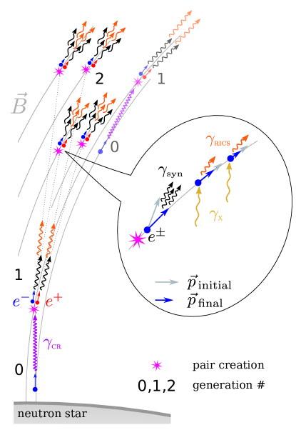
Figure 1: Schematic representation of electron-positron cascade in the polar cap of a young pulsar with high magnetic field, see text for description.

Fig. 1 gives a schematic overview of processes involved in pair plasma generation in PC cascades, shown are the first two generations in a cascade initiated by a primary electron. Primary electrons emit CR photons ($\gamma_{\textrm{\scriptsize{{cr}}}}$) almost tangent to the magnetic field lines; primary electrons and CR photons are generation 0 particles in our notation. Magnetic field lines are curved and the angle between the photon momentum and the magnetic field grows as the photon propagates further from the emission point. When this angle becomes large enough, photons are absorbed and each photon creates an electron-positron pair – generation 1 electron ($e^{-}$) and positron ($e^{+}$). The pair momentum is directed along the momentum of the parent photon and at the moment of creation, the particles have non-zero momentum perpendicular to the magnetic field. They radiate this perpendicular momentum almost instantaneously via SR and move along magnetic field lines. The secondary particles can scatter thermal X-ray photons $\gamma_{X}$ coming from the NS surface and lose their momenta parallel to the magnetic field. Inverse Compton Scattering of the thermal photons in the non-resonant regime is very ineffective in converting the energy of parallel motion of pairs into pair producing photons and can be neglected, see Appendix A. On the other hand, the RICS as it was first pointed out by Dermer (1990), can become a very efficient emission process in high field pulsars. Although the secondary particles are relativistic, their energy is much lower than that of the primaries and their curvature photons cannot create pairs. Generation 1 photons – synchrotron ($\gamma_{\textrm{\scriptsize{syn}}}$) and RICS ($\gamma_{\textrm{\scriptsize{{rics}}}}$) photons produced by the generation 1 particles are also emitted (almost) tangent to the magnetic field line – as the secondary particles are relativistic – and propagate some distance before acquiring the necessary angle to the magnetic field and creating generation 2 pairs. These pairs in their turn radiate their perpendicular momentum via SR, and parallel momenta via RICS emitting generation 2 photons. The cascade initiated by a single CR photon stops at a generation where the energy of synchrotron photons falls below $\epsilon_{\gamma,\,\textrm{\scriptsize{esc}}}$.

Primary particles emit pair producing CR photons throughout the whole cascade zone as they move along the field lines. Secondary particles emit all their pair producing synchrotron photons after their creation almost instantaneously. RICS photons are emitted by secondary particles over some distance, which is usually much smaller than the size of the cascade zone.

In the following sections we analyze the individual factors regulating the yield of electron-positron cascades and develop a semi-analytical technique which models cascade development by following the general picture outline above.

3 Photon absorption in magnetic field

3.1 Pair creation

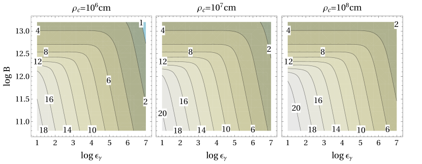
Figure 2: Contour plot of $1/\chi_{a}$ as a function of the logarithms of the magnetic field strength $B$ in Gauss, and photon energy $\epsilon_{\gamma}$ normalized to the electron rest energy, for three values of the radius of curvature of magnetic field lines $\rho_{\textrm{\scriptsize{c}}}=10^{6},10^{7},10^{8}\mbox{cm}$. $1\chi_{a}$ values shown on this plot are calculated from eq. (10).

For the opacity for single photon pair production in a strong magnetic field $\gamma\rightarrow{}e^{+}e^{-}$ we use the prescription suggested by Daugherty & Harding (1983) which can be written as

$$\alpha_{\gamma\rightarrow\pm}(\epsilon_{\gamma},\psi)=0.23\,\frac{\alpha_{f}}{\lambdabar{}_{\textrm{\scriptsize{{c}}}}}\>b\,\sin\psi\,\exp\left(-\frac{4}{3\chi}\right)\,f_{\alpha,1}\,.$$ (2)

where $b\equiv{}B/B_{q}$ is the local magnetic field strength $B$ normalized to the critical quantum magnetic field $B_{q}=e/\alpha_{f}\lambdabar{}_{\textrm{\scriptsize{{c}}}}^{2}=\mbox{$4.41\times 10^{13}$}$ G, $\psi$ is the angle between the photon momentum and the local magnetic field, $\alpha_{f}=e^{2}/\hbar{}c\approx{}1/137$ is the fine structure constant, and $\lambdabar{}_{\textrm{\scriptsize{{c}}}}=\hbar/mc=\mbox{$3.86\times 10^{-11}$}$ cm is the reduced Compton wavelength. The parameter $\chi$ is defined as

$$\chi\equiv\frac{1}{2}\,\epsilon_{\gamma}b\,\sin\psi\,,$$ (3)

where $\epsilon_{\gamma}$ is the photon energy in units of $m_{e}c^{2}$. Expression (2) differs from the usual Erber (1966) formula by the term

$$f_{\alpha,1}=\begin{cases}\displaystyle\exp\left(-0.56\,\frac{b^{2.6962}}{\chi^{3.7}}\right),&\text{ if }\epsilon_{\gamma}\sin\psi\geq 2\\ 0,&\text{ if }\epsilon_{\gamma}\sin\psi<2\end{cases}$$ (4)

The function $f_{\alpha,1}$ insures that the attenuation coefficient for pair production becomes zero below the threshold $\epsilon_{\gamma}\sin\psi=2$ and corrects $\alpha_{\gamma\rightarrow\pm}$ for the case when absorption happens hear the threshold. The threshold condition for $\gamma{}B$ pair production can be expressed in terms of $\chi$ as

$$\chi\geq{}b\,.$$ (5)

Expression (2) works for high, $B>\mbox{$3\times 10^{12}$}$G, magnetic fields, for weaker fields it reduces to the well known Erber’s formula (see Appendix B).

The optical depths for pair creation by a high energy photon in a strong magnetic field after propagating distance $l$ is

$$\tau(\epsilon_{\gamma},l)=\int_{0}^{l}\alpha_{\gamma\rightarrow\pm}(\epsilon_{\gamma},\psi(x))\,dx\,,$$ (6)

where integration is along the photon’s trajectory. For photons emitted tangent to the magnetic field line, $dx=\rho_{\textrm{\scriptsize{c}}}d\psi$, where $\rho_{\textrm{\scriptsize{c}}}$ is the radius of curvature of magnetic field lines. From eq. (3) we have $\psi=2\chi/\epsilon_{\gamma}{}b$, and substituting it into eq. (6) we can express the optical depth $\tau$ to pair production as an integral over $\chi$ as

$$\tau(\epsilon_{\gamma},\tilde{\chi})=\frac{A_{\tau}}{\epsilon_{\gamma}^{2}}\;\int_{0}^{\tilde{\chi}}\frac{\rho_{\textrm{\scriptsize{c}}}}{b}\chi\exp\left(-\frac{4}{3\chi}\right)\,f_{\alpha,1}\,d\chi\,,$$ (7)

where $A_{\tau}\equiv{}0.92\alpha_{f}/\lambdabar{}_{\textrm{\scriptsize{{c}}}}\approx\mbox{$1.74\times 10^{8}$}\;\mbox{cm}^{-1}$ . The optical depth depends exponentially on $\chi$ and the main contribution to the integral comes from the values of $\chi$ close to the upper boundary $\tilde{\chi}$. For a wide range of photon energies and field strengths the value of $\chi$ at the point where the photon is absorbed $\chi_{a}$, changes slowly. The mean free path of photons can be estimated from eq. (3) as

$$\lambda_{\gamma\rightarrow\pm}=2\rho_{\textrm{\scriptsize{c}}}\chi_{a}\frac{1}{b\epsilon_{\gamma}}\,.$$ (8)

Both $\chi_{a}$ and $\rho_{\textrm{\scriptsize{c}}}$ change slower than $b$ and $\epsilon_{\gamma}$ as the cascade develops. In each cascade generation the energy of particles and photons is smaller than that in the preceding generation. The photon mean free path $\lambda_{\gamma\rightarrow\pm}$ increases because of this. If $\lambda_{\gamma\rightarrow\pm}$ becomes comparable to the characteristic scale of the magnetic field variation $L_{B}$, then the increase of $\lambda_{\gamma\rightarrow\pm}$ for the next generation photons will be compounded by additional decrease of the magnetic field $b$ as well, by at least $\sim$an order of magnitude (for dipolar field). In most cases the magnetic field at the anticipated absorption point for the next generation of photons will drop below the pair formation threshold (5). Hence, the cascade generation for which $\lambda_{\gamma\rightarrow\pm}\sim{}L_{B}$ should be the final one.

We consider strong cascades with large multiplicities; such cascades fully develop before $\lambda_{\gamma\rightarrow\pm}\sim{}L_{B}$. For such cascades in the region where most of the pairs are produced the magnetic field $b$ and the radius of curvature of magnetic field lines $\rho_{\textrm{\scriptsize{c}}}$ are approximately constant. In approximation of constant $b$ and $\rho_{\textrm{\scriptsize{c}}}$ eq. (7) can be written as

$$\tau(\chi)=A_{\tau}\frac{\rho_{\textrm{\scriptsize{c}}}}{\epsilon_{\gamma}^{2}\,b}\;\int_{0}^{\chi_{a}}\chi\exp\left(-\frac{4}{3\chi}\right)\,f_{\alpha,1}\,d\chi\,$$ (9)

and integrated analytically. The resulting expression is quite cumbersome, it is derived in Appendix B, and given by eq. (B11).

Because the opacity to pair production depends exponentially on $\chi$ it is a reasonable approximation that all photons are absorbed when they have traveled the distance where $\tau=1$. We define $\chi_{a}$ as the value of $\chi$ where the optical depth reaches 1 through

$$\chi_{a}:\tau(\chi_{a})=1\,.$$ (10)

$\chi_{a}$ is a solution of the non-linear equation (10) with $\tau$ given by eq. (B11). We solved equation (10) numerically for different values of $\epsilon_{\gamma}$, $b$, and $\rho_{\textrm{\scriptsize{c}}}$. In Fig. 2 we plot contours of $1/\chi_{a}$ as functions of $\log(\epsilon_{\gamma})$ and $\log(B)$ for three different values for the radius of curvature of the magnetic field lines $\rho_{\textrm{\scriptsize{c}}}=10^{6},10^{7},10^{8}\mbox{cm}$. The smallest value of $\rho_{\textrm{\scriptsize{c}}}$ corresponds to a strongly multipolar polar cap magnetic field, when the radius of curvature is comparable to the NS radius. The largest value corresponds to the radius of curvature of dipolar magnetic field lines, which at the NS surface is given by

$$\rho_{\textrm{\scriptsize{c, dip}}}=\frac{4}{3}\frac{R_{\textrm{\scriptsize{{ns}}}}}{\theta}=\mbox{$9.2\times 10^{7}$}\left(\frac{\theta}{\theta_{\textrm{\scriptsize{pc}}}}\right)^{-1}P^{1/2}\,\mbox{cm}\,,$$ (11)

where $\theta$ is the colatitude of the footpoint of the magnetic field line, $\theta_{\textrm{\scriptsize{pc}}}=\mbox{$1.45\times 10^{-2}$}P^{-1/2}$ – the colatitude of the polar cap boundary, $P$ – the pulsar period in seconds, and $R_{\textrm{\scriptsize{{ns}}}}=10^{6}$cm – the NS radius.

$1/\chi_{a}$ is a smooth function of $\log(\epsilon_{\gamma})$, $\log(B)$, and $\log\rho_{\textrm{\scriptsize{c}}}$ – as it is to be expected from $\alpha_{\gamma\rightarrow\pm}\propto\exp(-1/\chi)$ – and can be accurately approximated using a modest size numerical table. The change in the behavior of $1/\chi_{a}$ for large magnetic fields, when the contour lines become horizontal, is due to photon being absorbed close to the pair production threshold eq. (5).

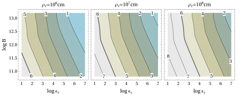
Figure 3: Contour plot of the logarithm of the photon mean free path $\log\lambda_{\gamma\rightarrow\pm}$ (in cm) as a function of the logarithms of the magnetic field strength $B$ in Gauss, and photon energy $\epsilon_{\gamma}$ normalized to the electron rest energy, for three values of the radius of curvature of magnetic field lines $\rho_{\textrm{\scriptsize{c}}}=10^{6},10^{7},10^{8}\mbox{cm}$. $\log\lambda_{\gamma\rightarrow\pm}$ values shown on this plot are calculated from eq. (8).

The values of $\chi_{a}$ we obtained here using a more accurate expression for the $\gamma{}B$ opacity, eq. (B11), are up to 40% higher than that from Pap I where we used Erber’s formula and made a simple correction for the pair formation threshold by setting the upper limit on $\chi$ according to eq. (5). This difference is larger that 10% only for magnetic fields with $B\gtrsim\mbox{$1.5\times 10^{12}$}$G (cf. Fig. 2 with Fig.3 from Pap I). Also note that the values of $\chi_{a}$ differ significantly from the often used value $\chi_{a}=1/15$ first suggested by Ruderman & Sutherland (1975), especially for higher energy photons.

The contour plots of the mean free path of the photons $\lambda_{\gamma\rightarrow\pm}$ emitted tangentially to the magnetic field lines are shown on Fig. 3; $\lambda_{\gamma\rightarrow\pm}$ was calculated according to eq. (8). As expected it scales linearly with $1/\epsilon_{\gamma}$ and $1/B$, the deviation from the linear behavior is seen only for the combination of $\epsilon_{\gamma}$ and $B$ when pair formation happens near the threshold, at $B\gtrsim\mbox{$1.5\times 10^{12}$}$G.

3.2 Photon splitting

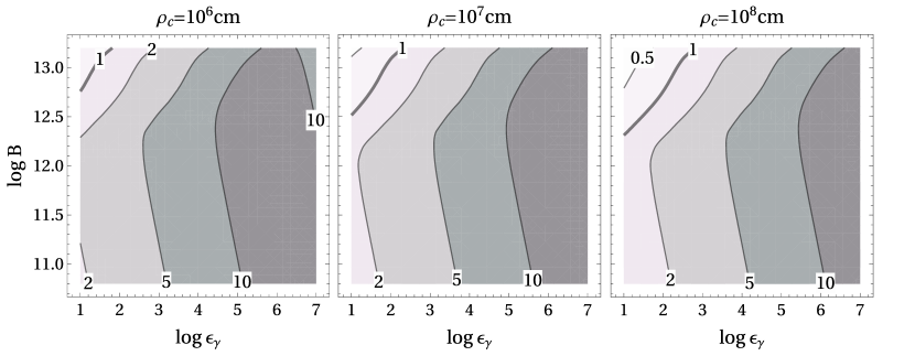
Figure 4: Contour plot of the ratio of mfp for photon splitting to the mfp for pair production $\lambda_{\gamma\rightarrow\gamma\gamma}/\lambda_{\gamma\rightarrow\pm}$ (in linear scale) as a function of the logarithms of the magnetic field strength $B$ in Gauss, and photon energy $\epsilon_{\gamma}$ normalized to the electron rest energy, for three values of the radius of curvature of magnetic field lines $\rho_{\textrm{\scriptsize{c}}}=10^{6},10^{7},10^{8}\mbox{cm}$.

Single photon pair creation is not the only process responsible for photon attenuation in strong magnetic field, albeit the most significant one. The most important competing process to pair creation is magnetic photon splitting $\gamma\rightarrow\gamma\gamma$. Besides the end product, the major differences between pair creation and photon splitting are: (i) pair creation is a first order QED process and splitting is a third order one, therefore splitting is weaker than pair creation by the order of $\alpha_{f}^{2}$; (ii) in contrast to pair creation, splitting has no threshold for photon’s energy; (iii) while in moderately strong magnetic fields $B\lesssim B_{\textrm{\scriptsize{cr}}}$ for pair creation both modes of photon polarization ($\parallel$ – when photon’s electric field is parallel to the plane containing $\vec{B}$ and photon’s momentum, $\perp$ – photon’s electric field is perpendicular to that plane) have similar cross-sections and threshold conditions, below pair formation threshold photon splitting is allowed only for the process $\perp\rightarrow\parallel\parallel$ (Adler, 1971; Usov, 2002).

Radiation processes relevant for secondary particles in polar cap cascades of energetic pulsars (SR, RICS) produce predominantly $\perp$ polarized photons. Despite the inherently smaller cross-section of magnetic splitting, the absence of an energy threshold could allow photons to split before acquiring large enough angles to the magnetic field to produce pairs, thus reducing cascade multiplicity. As we are interested in the most efficient cascades, a regime where magnetic splitting becomes important is beyond the scope of this paper. More details on cascade kinetics in the presence of photon splitting can be found in Harding et al. (1997); Baring & Harding (1997, 2001). Here we want to establish the boundary in the parameter space where photons splitting start affecting cascade multiplicity. To do so we consider a case of photon splitting $\perp\rightarrow\parallel\parallel$ for photons below pair formation threshold.

The attenuation coefficient for photon splitting $\perp\rightarrow\parallel\parallel$ is (Baring, 2008; Baring & Harding, 2001)

$$\alpha_{\gamma\rightarrow\gamma\gamma}(\epsilon_{\gamma},\psi)=\frac{\alpha_{f}^{3}c}{60\pi^{2}\lambdabar{}_{\textrm{\scriptsize{{c}}}}}\epsilon_{\gamma}^{5}b^{6}\sin\psi^{6}\mathcal{M}_{1}^{2}$$ (12)

at low values of the magnetic field perpendicular to the photon’s trajectory – for photons below the pair formation threshold – the scattering amplitude $\mathcal{M}_{1}$ is a constant independent of $b$ $\mathcal{M}_{1}\approx 26/315$. Integration of $\alpha_{\gamma\rightarrow\gamma\gamma}$ over the distance gives the optical depth for photon splitting (cf. eq. (6)); the mfp for splitting can then be estimated as

$$\lambda_{\gamma\rightarrow\gamma\gamma}=1.8\,\epsilon_{\gamma}^{-5/7}b^{-6/7}\rho_{\textrm{\scriptsize{c}}}^{6/7}\,\mbox{cm}$$ (13)

When the mfp for splitting becomes smaller than the mfp for pair formation, $\lambda_{\gamma\rightarrow\gamma\gamma}<\lambda_{\gamma\rightarrow\pm}$, the photon splits before producing a pair. In Fig. 4 we plot the ratio $\lambda_{\gamma\rightarrow\gamma\gamma}/\lambda_{\gamma\rightarrow\pm}$ as a function of magnetic field strength and photon energy, for three values of the radius of curvature of magnetic field lines. It is evident from these plots, splitting is an important attenuation mechanism only for strong magnetic fields and low energy photons. With the increase of the magnetic field, photon splitting starts affecting first the last cascade generation where the energy of the photons becomes low. If these photons split, the resulting photons will be below pair formation threshold. In the polar cap cascades most of the pairs are produced in the last cascade generation, and when photon splitting becomes important, the cascade multiplicity can drop significantly. The exact fraction of perpendicularly polarized photons in the cascade – which are subject to splitting – in general depends on particle energy distributions, but it is more than %50 (e.g. Baring & Harding, 2001). Hence, the multiplicity of the pair cascade will drop by at least a factor of 2 when photon splitting becomes important.

The critical magnetic field strength $B_{\gamma\rightarrow\gamma\gamma}$ above which cascade multiplicity becomes affected by photon splitting is the field strength when $\lambda_{\gamma\rightarrow\gamma\gamma}<\lambda_{\gamma\rightarrow\pm}$ for the last generation photons, i.e. at for photons with the escaping energy $\epsilon_{\gamma,\,\textrm{\scriptsize{esc}}}$ (which we calculate in the next section)

$$B_{\gamma\rightarrow\gamma\gamma}:\lambda_{\gamma\rightarrow\gamma\gamma}(\epsilon_{\gamma,\,\textrm{\scriptsize{esc}}})=\lambda_{\gamma\rightarrow\pm}(\epsilon_{\gamma,\,\textrm{\scriptsize{esc}}})\,.$$ (14)

3.3 Energy of escaping photons

As we discussed above, photons escaping the cascade are those with mfp larger than the characteristic scale of magnetic field variation $\lambda_{\gamma\rightarrow\pm}>L_{B}$. The formal criteria we use to calculate the energy of escaping photons $\epsilon_{\gamma,\,\textrm{\scriptsize{esc}}}$ is $\lambda_{\gamma\rightarrow\pm}(\epsilon_{\gamma,\,\textrm{\scriptsize{esc}}})=s_{\textrm{\scriptsize{esc}}}R_{\textrm{\scriptsize{{ns}}}}$; $s_{\textrm{\scriptsize{esc}}}$ is a dimensionless parameter quantifying the escaping distance in units of $R_{\textrm{\scriptsize{{ns}}}}$. From the expression for mfp, eq. (8), we get a (non-linear) equation for $\epsilon_{\gamma,\,\textrm{\scriptsize{esc}}}$

$$\epsilon_{\gamma,\,\textrm{\scriptsize{esc}}}=2\,\frac{\rho_{\textrm{\scriptsize{c}}}}{s_{\textrm{\scriptsize{esc}}}R_{\textrm{\scriptsize{{ns}}}}}\frac{\chi_{a}}{b}\,.$$ (15)

Any global NS magnetic field near the surface decays with distance as $(r/R_{\textrm{\scriptsize{{ns}}}})^{-\delta}$, $\delta\geq 3$; a dipole field, $\delta=3$, is often considered as a reasonable assumption. A pure dipole, however, seems to be too idealized an approximation, as the NS magnetic field is slightly disturbed by the currents flowing in the magnetosphere. Polar cap cascade models should consider at least near dipole magnetic fields with different curvatures of magnetic field lines. Hence, a reasonable estimate for $L_{B}$ would be the distance of the order of the NS radius $R_{\textrm{\scriptsize{{ns}}}}$. For our approximation of constant $B$ and $\rho_{\textrm{\scriptsize{c}}}$ we found that the value $L_{B}=R_{\textrm{\scriptsize{{ns}}}}/2$ – at that distance from the NS the magnetic field decays by at least the factor of 3 – provides a good fit to the results of numerical simulations described in Pap I. Results described in this paper are obtained assuming $s_{\textrm{\scriptsize{esc}}}=0.5$.

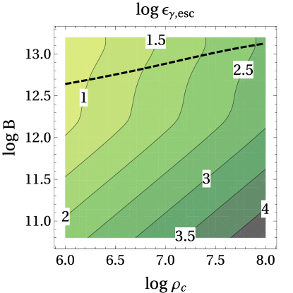
Figure 5: Energy of escaping photons: contours of $\log{\epsilon_{\gamma,\,\textrm{\scriptsize{esc}}}}$ as a function of logarithms of the radius of curvature of magnetic field lines $\rho_{\textrm{\scriptsize{c}}}$ in cm and magnetic field strength $B$ in Gauss for $s_{\textrm{\scriptsize{esc}}}=1$. The critical magnetic field $B_{\gamma\rightarrow\gamma\gamma}$ above which photon splitting starts affecting cascade multiplicity is shown by the dashed line.

In Fig. 5 we plot the energy of escaping photons, $\log{\epsilon_{\gamma,\,\textrm{\scriptsize{esc}}}}$ as a function of the radius of curvature of magnetic field lines $\rho_{\textrm{\scriptsize{c}}}$ and magnetic field strength $B$ for $s_{\textrm{\scriptsize{esc}}}=1$. This figure shows (an obvious) trend that for higher magnetic field and smaller radii of curvature, the energy of escaping photons is lower. The deviation of contours from straight lines for $B\gtrsim\mbox{$3\times 10^{12}$}$G is due to the change of $\chi_{a}$ behavior near the pair formation threshold (see Fig. 2 and the next paragraph). For different values of $s_{\textrm{\scriptsize{esc}}}$ the escape energy $\epsilon_{\gamma,\,\textrm{\scriptsize{esc}}}$ could be estimated from Fig. 3.

The critical magnetic field $B_{\gamma\rightarrow\gamma\gamma}$ above which photon splitting starts affecting cascade multiplicity is shown in Fig. 5 by the dashed line, $B_{\gamma\rightarrow\gamma\gamma}$ is calculated from eq. (14). Cascade multiplicity will drop due to photon splitting at $B\gtrsim\mbox{$4.4\times 10^{12}$}$G for $\rho_{\textrm{\scriptsize{c}}}=10^{6}$cm, and at $B\gtrsim\mbox{$1.3\times 10^{13}$}$G for $\rho_{\textrm{\scriptsize{c}}}=10^{8}$cm. The increase of $B_{\gamma\rightarrow\gamma\gamma}$ for larger $\rho_{\textrm{\scriptsize{c}}}$ is due to the increase of the energy of escaping photons – $\lambda_{\gamma\rightarrow\pm}$ has stronger dependence on $\epsilon_{\gamma}$ than $\lambda_{\gamma\rightarrow\gamma\gamma}$, that leads to the increase of the value $B_{\gamma\rightarrow\gamma\gamma}$ according to eqs. (14), (13), (8).

Figure 6: Contour plot of $\chi_{\textrm{\scriptsize{a,esc}}}$ as a function of the logarithms of the magnetic field strength $B$ in Gauss, and the radius of curvature of magnetic field lines $\rho_{\textrm{\scriptsize{c}}}$.

It would be useful to have an analytical expression for the energy of escaping photons; to obtain it we construct an approximation for $\chi_{a,\,\textrm{\scriptsize{esc}}}$. We solved eq. (15) to find $\epsilon_{\gamma,\,\textrm{\scriptsize{esc}}}$; now, using the interpolation formula for $1/\chi_{a}$, we can find $1/\chi_{a,\,\textrm{\scriptsize{esc}}}\equiv{}1/\chi_{a}(\epsilon_{\gamma,\,\textrm{\scriptsize{esc}}})$. In Fig. 6 we show contours of $1/\chi_{a,\,\textrm{\scriptsize{esc}}}$ as a function of $B$ and $\rho_{\textrm{\scriptsize{c}}}$. There are two distinct regions on this plot: for $B\gtrsim\mbox{$3\times 10^{12}$}$G $\chi_{a,\,\textrm{\scriptsize{esc}}}$ changes very slowly, while for larger values of B it changes significantly but does not depend on $\rho_{\textrm{\scriptsize{c}}}$. For $B\gtrsim\mbox{$3\times 10^{12}$}$G the absorption of the last generation photons happens near the pair formation threshold, when $\epsilon_{\perp}=\epsilon_{\gamma,\,\textrm{\scriptsize{esc}}}(R_{\textrm{\scriptsize{{ns}}}}/\rho_{\textrm{\scriptsize{c}}})\simeq 2$, and so $\chi_{a,\,\textrm{\scriptsize{esc}}}\simeq{}b$. For weaker magnetic fields the opacity for near-threshold photons are too small for them to be absorbed after traveling the distance $R_{\textrm{\scriptsize{{ns}}}}$, so the last generation photons have energies larger than the pair formation threshold and are absorbed at very similar values of $\chi_{a}$. We find that the following approximation work quite well

$$\chi_{a,\,\textrm{\scriptsize{esc}}}=\begin{cases}b,&\text{if $b>1/15$}\\ 1/15,&\text{if $b\leq 1/15$}\end{cases}$$ (16)

The energy of the escaping photons can be expressed from eq. (15) as

$$\epsilon_{\gamma,\,\textrm{\scriptsize{esc}}}\approx{}\mbox{$1.8\times 10^{3}$}\,\frac{\rho_{\textrm{\scriptsize{c,7}}}}{B_{12}}\left(\frac{s_{\textrm{\scriptsize{esc}}}}{0.5}\right)^{-1}\chi_{a,\,\textrm{\scriptsize{esc}}}\;,$$ (17)

where $\chi_{a,\,\textrm{\scriptsize{esc}}}$ is given by eq. (16) and $B_{12}\equiv{}B/10^{12}$G and $\rho_{\textrm{\scriptsize{c,7}}}\equiv\rho_{\textrm{\scriptsize{c}}}/10^{7}$cm. This simple prescription for $\epsilon_{\gamma,\,\textrm{\scriptsize{esc}}}$ deviates from numerical values shown in Fig. 5 by no more than 20% for $B\lesssim\mbox{$2\times 10^{12}$}$G and $B\gtrsim\mbox{$8\times 10^{12}$}$G, the largest deviation is $\sim 60\%$ at $B\simeq\mbox{$3\times 10^{12}$}$G.

For very small values of $\chi_{a,\,\textrm{\scriptsize{esc}}}$ it is possible to get a more accurate analytical expression for $\chi_{a,\,\textrm{\scriptsize{esc}}}$ (and $\epsilon_{\gamma,\,\textrm{\scriptsize{esc}}}$). Using asymptotic expression for the optical depth in the limit of $\chi\ll 1$ derived in Appendix B, eq. (B13) and substituting for the photon energy the energy of escaping photons eq. (15) we get

$$\frac{1}{\chi_{a,\,\textrm{\scriptsize{esc}}}} \approx\frac{3}{4}\ln\left(\frac{3A_{\tau}R_{\textrm{\scriptsize{{ns}}}}^{2}}{16}\frac{b}{\rho_{\textrm{\scriptsize{c}}}}\chi_{a,\,\textrm{\scriptsize{esc}}}\,s_{\textrm{\scriptsize{esc}}}^{2}\right)$$ (18)

$$\approx 15.7+1.7\log\left(\frac{B_{12}}{\rho_{7}}\right)+3.5\log\left(\frac{s_{\textrm{\scriptsize{esc}}}}{0.5}\right)$$

4 Particle acceleration

Self-consistent modeling of accelerating zones in pulsar polar caps (Timokhin, 2010; Timokhin & Arons, 2013) demonstrated that particle acceleration and pair formation are always non-stationary. Each period of intense particle acceleration and pair formation is followed by a period of quiet plasma flow when the accelerating electric field is screened and no pairs are formed. At the end of the quiet phase an accelerating gap begins to form – a region where plasma density is significantly smaller than the local GJ number density $\eta_{\textrm{\scriptsize{{gj}}}}/e$. Accelerating electric field in the gap increases linearly with distance as the gap grows. Charged particles entering the gap are accelerated to very high energies and emit gamma-rays which give rise to electron-positron pair cascades. Dense pair plasma created in the cascades screens the electric field, stopping the growth of the gap. The gap does not stay at the same place, but moves along magnetic field lines roughly preserving its size (and the potential drop) for a while. Most of the pair plasma is created at or behind the trailing edge of the gap, where the high energy particles are located. These particles move into the magnetosphere, emitting gamma-rays which convert into electron positron pairs. Both primary and secondary particles are relativistic and so they move together, forming a blob of pair plasma those density increases as pair formation continues. Some low energy particles, however, “leak” from the blob, creating a tail of mildly relativistic plasma which screens the electric field behind the blob. When the blob with primary particles move away from the polar cap and pair formation stops, the dense pair plasma from the tail keeps the electric field screened for a while until most of it has left the polar cap zones and a new cycle of pair formation begins.

Whether and how efficient the pair formation along given magnetic field lines occurs depends on the ratio $j_{\textrm{\scriptsize{m}}}/j_{\textrm{\scriptsize{{gj}}}}$ of the current density required to support the twist of magnetic field lines in the pulsar magnetosphere (e.g. Timokhin, 2006; Bai & Spitkovsky, 2010), $j_{\textrm{\scriptsize{m}}}\equiv(c/4\pi)\,|\nabla\times\mathbf{B}|$, to the local GJ current density, $j_{\textrm{\scriptsize{{gj}}}}\equiv\eta_{\textrm{\scriptsize{{gj}}}}c$, where $\eta_{\textrm{\scriptsize{{gj}}}}=B/Pc$ is the GJ charge density. Regardless of the ability of the NS surface to supply charged particles, i.e. in both the space charge limited flow model of Arons & Scharlemann (1979) and the no-particle extraction model of Ruderman & Sutherland (1975), particle acceleration happens in essentially the same way. For the Ruderman & Sutherland (1975) regime effective particle acceleration and pair formation is possible for almost all values of $j_{\textrm{\scriptsize{m}}}/j_{\textrm{\scriptsize{{gj}}}}$. In the space charge limited flow regime pair formation is not possible if $0<j_{\textrm{\scriptsize{m}}}/j_{\textrm{\scriptsize{{gj}}}}<1$, but is possible for all other values of $j_{\textrm{\scriptsize{m}}}/j_{\textrm{\scriptsize{{gj}}}}$. A detailed description of particle acceleration in pulsar polar caps is given in Timokhin (2010) for the no-particle extraction regime and in Timokhin & Arons (2013) for the space charge limited flow regime.

Although the character of plasma flow inferred from self-consistent simulation of Timokhin (2010) and Timokhin & Arons (2013) qualitatively differs from that assumed in both Ruderman & Sutherland (1975) and Arons & Scharlemann (1979) type models, the physics of particle acceleration in the gap is similar to that of the accelerating gap in the Ruderman & Sutherland (1975) model. Namely, due to significant deviation of the charge and current densities from GJ values, the electric field in the gap is comparable to the vacuum electric field ($\sim{}h\Omega{}B/c$, $h$ is the size of the gap) and particles are accelerated in a short gap by the strong electric field which increases linearly with the distance. In §6.2 of Pap I we analyzed the physics of particle acceleration and derived an analytical expression for the energy of the primary particles accelerated in non-stationary cascades. According to eq. (41) in Pap I the final energy of particles accelerated in the gap

$$\epsilon_{\pm,\,\textrm{\scriptsize{acc}}} = \frac{49}{18}\left(\frac{\pi B_{q}}{\lambdabar{}_{\textrm{\scriptsize{{c}}}}^{3}c}\right)^{1/7}\chi_{a,\,\textrm{\scriptsize{acc}}}^{2/7}\;\xi_{j}^{1/7}P^{-1/7}B^{-1/7}\rho_{\textrm{\scriptsize{c}}}^{4/7}$$ (19)

$$\simeq \mbox{$5\times 10^{7}$}\>\chi_{a,\,\textrm{\scriptsize{acc}}}^{2/7}\;\xi_{j}^{1/7}P^{-1/7}B_{12}^{-1/7}\rho_{\textrm{\scriptsize{c,\,7}}}^{4/7}\,.$$

$\chi_{a,\,\textrm{\scriptsize{acc}}}$ is the value of the parameter $\chi$ for photons which create pairs terminating the gap. $\xi_{j}$ is a factor which shows how stronger/weaker the electric field in the gap is compared to the field in a static vacuum gap of an aligned rotator:

$$\xi_{j}\equiv\frac{|j-j_{\textrm{\scriptsize{m}}}|}{j_{\textrm{\scriptsize{{gj}}}}^{0}}\left(1+\frac{c}{v}\right)\approx{}2\,\frac{j_{\textrm{\scriptsize{m}}}}{j_{\textrm{\scriptsize{{gj}}}}^{0}}\,.$$ (20)

where $j$ is the current density in the gap. In most cases $|j-j_{\textrm{\scriptsize{m}}}|\simeq j_{\textrm{\scriptsize{m}}}$; $j_{\textrm{\scriptsize{{gj}}}}^{0}$ is the GJ current density in an aligned rotator

$$j_{\textrm{\scriptsize{{gj}}}}^{0}\equiv\eta_{\textrm{\scriptsize{{gj}}}}^{0}c=\frac{B}{P}\,.$$ (21)

$v$ is the velocity of the gap; in most cases the gap moves with relativistic velocities, so $v\simeq{}c$. Taking into account these approximations we get the second expression for $\xi_{j}$ in eq. (20). $j_{\textrm{\scriptsize{m}}}$, and so $\xi_{j}$, depend on the pulsar inclination angle and the position of the given magnetic field line inside the polar cap (see e.g. Fig. 1 in Timokhin & Arons (2013)). In cascades along magnetic field lines where $j_{\textrm{\scriptsize{m}}}$ is close to the local value of $j_{\textrm{\scriptsize{{gj}}}}$ in an aligned rotator $\xi_{j}\sim 2$, for the same situation in a pulsar with inclination angle of $60^{\circ}$, $\xi_{j}\sim 1$. The energy of primary particles eq. (19) has the same dependence on $\rho_{\textrm{\scriptsize{c}}}$, $P$ and $B$ as the expression for the potential drop in the gap derived by Ruderman & Sutherland (1975), their eq. (23). This is to be expected as in both cases particles are accelerated by the electric field which grows linearly with the distance and the size of the gap is regulated by absorption on curvature photons in magnetic field. The difference is in the presence of factor $\xi_{j}$ and a different numerical factor.

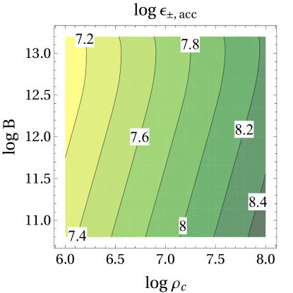
Figure 7: Primary particle energy: contours of $\log\epsilon_{\pm,\,\textrm{\scriptsize{acc}}}$ as a function of logarithms of the radius of curvature of magnetic field lines $\rho_{\textrm{\scriptsize{c}}}$ in cm and magnetic field strength $B$ in Gauss. We used the following values for gap parameters $P=33$ ms, $\xi_{j}=2$.

Figure 8: Contour plot of $1/\chi_{a,\,\textrm{\scriptsize{acc}}}$ as a function of logarithms of the radius of curvature of magnetic field lines $\rho_{\textrm{\scriptsize{c}}}$ in cm and magnetic field strength $B$ in Gauss. We used the following values for gap parameters $P=33$ ms and $\xi_{j}=2$.

Here we slightly improve the accuracy of this expression by calculating self-consistently the value of the parameter $\chi_{a,\,\textrm{\scriptsize{acc}}}$. Using numerical interpolation for $\chi$ (see §3.1) it is easy to obtain self-consistently the energy of primary particles accelerated in the gap $\epsilon$ by solving numerically the equation

$$\epsilon_{\pm,\,\textrm{\scriptsize{acc}}}(\chi_{a,\,\textrm{\scriptsize{acc}}}(\epsilon))=\epsilon\,,$$ (22)

i.e. to find the energy of particles which emit photons terminating the gap growth taking into account the dependence of $\chi_{a,\,\textrm{\scriptsize{acc}}}$ on particle energy (via the energy of emitted photons). In Fig. 7 we show the energy of accelerated particles for a pulsar with $P=33$ ms. The contours of constant $\chi_{a,\,\textrm{\scriptsize{acc}}}$ deviate only slightly from straight lines corresponding to $\propto\rho_{\textrm{\scriptsize{c}}}^{4/7}B^{-1/7}$ for higher values of $B$. This deviation is due to variation of $\chi_{a,\,\textrm{\scriptsize{acc}}}$ near the pair formation threshold and so the expression (19) can be safely used in many cases with a constant value of $\chi_{a,\,\textrm{\scriptsize{acc}}}$. $\chi_{a,\,\textrm{\scriptsize{acc}}}$ itself varies slowly with gap parameters. In Fig. 8 we show $1/\chi_{a,\,\textrm{\scriptsize{acc}}}$ for a pulsar with $P=33$ ms; it was obtained together with values from eq. (22). It is evident that the value of $\chi_{a,\,\textrm{\scriptsize{acc}}}=1/5.5$ can be used in eq. (19) for pulsars with $P=33$ ms. The dependence of $\chi_{a,\,\textrm{\scriptsize{acc}}}$ on pulsar period $P$ and parameter $\xi_{j}$ is also quite weak, see in Table 1 where we show the variation of $\chi_{a,\,\textrm{\scriptsize{acc}}}$ at $B=10^{12}$G, $\rho_{\textrm{\scriptsize{c}}}=10^{7}$cm with $P$ and $\xi_{j}$ and for estimates of the primary particle energies one can use $\chi_{a,\,\textrm{\scriptsize{acc}}}=1/7$. The dependence of the particle energy is weak and along most of magnetic field line in the polar cap $\xi_{j}$ is no more than $\sim$an order of magnitude lower than 2. Assuming $\chi_{a,\,\textrm{\scriptsize{acc}}}=1/7$ and $\xi_{j}=2$ eq. (19) can be written

$$\epsilon_{\pm,\,\textrm{\scriptsize{acc}}}\simeq\mbox{$3.2\times 10^{7}$}\>P^{-1/7}B_{12}^{-1/7}\rho_{\textrm{\scriptsize{c,\,7}}}^{4/7}\,.$$ (23)

This estimate for the primary particle energy can be used for a wide rage of parameters of young energetic pulsars. It is $\simeq 4$ times higher than the that given by eq. (23) in Ruderman & Sutherland (1975).

P	ξ_j=0.25	ξ_j=2
0.033	6.6	5.5
0.33	7.9	6.6

Table 1: $1/\chi_{a,\,\textrm{\scriptsize{acc}}}$ for $B=10^{12}$G, $\rho_{\textrm{\scriptsize{c}}}=10^{7}$cm and different values of $P$ and $\xi_{j}$

The primary particle energy has a weak dependence on pulsar period, inclination angle (via $\xi_{j}$), and magnetic field strength; its strongest dependence is on the radius of curvature of magnetic field lines. These trends are consequences of the fact that the potential drop across the acceleration gap is regulated by pair formation. The gap terminates when particles reach energies high enough to emit pair producing photons. A gap with weak accelerating electric field due to e.g. weaker magnetic field and/or longer period and/or smaller current density $j_{\textrm{\scriptsize{m}}}$ will have larger height than a gap with strong accelerating field, to accelerate particles to the energies when they emit pair producing photons. A larger height of the gap also results in longer distances traveled by photons; this largely alleviates the dependence of the energy of the pair producing photons on the magnetic field strength, leaving the curvature of magnetic field lines as the strongest factor determining the energy of primary particles.

5 The maximum pair multiplicity: simple estimate

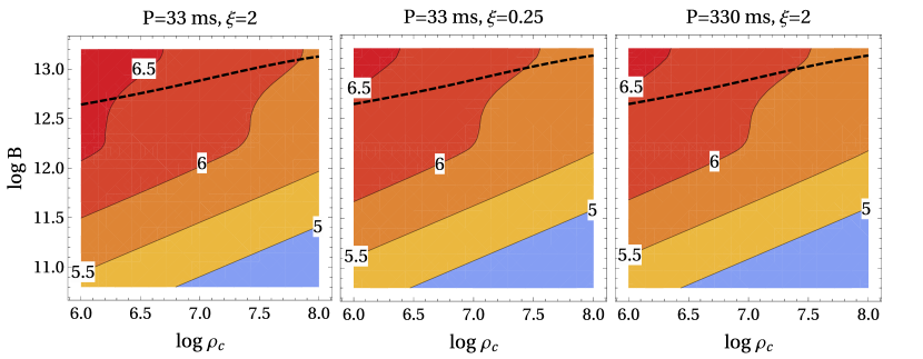
Figure 9: Simple estimate for the maximum multiplicity of polar cap cascades: contours of $\log\kappa_{\textrm{\scriptsize{max}}}$ as a function of logarithms of curvature of magnetic field lines $\rho_{\textrm{\scriptsize{c}}}$ in cm and magnetic field strength $B$ in Gauss for three sets of the gap parameters $(P[\mbox{s}],\xi_{j})$: $(0.033,2)$, $(0.033,0.25)$, $(0.33,2)$. The critical magnetic field $B_{\gamma\rightarrow\gamma\gamma}$ above which photon splitting starts affecting cascade multiplicity is shown by the dashed line.

Now we can make a simple estimate of the maximum cascade multiplicity during a burst of pair creation. As discussed in §2, in a hypothetical ideal cascade the whole kinetic energy of the primary particle is divided into energies of pairs which are produced by the photons with the energies just above the escape energy; in such a cascade the multiplicity is given by eq. (1) – twice the energy of the primary particle divided by the energy of escaping photons. In Fig. 9 we show the estimates for the multiplicity of an ideal cascade $\log\kappa_{\textrm{\scriptsize{max}}}$ as a function of the magnetic field strength and the radius of curvature of the magnetic field lines for three sets of the gap parameters $(P[\mbox{s}],\xi_{j})$: $(0.033,2)$, $(0.033,0.25)$, $(0.33,2)$ . Energies of primary particles and escaping photons are calculated according to §§ 3.3, 4. The maximum cascade multiplicity is not very sensitive to pulsar period and inclination angle (via $\xi_{j}$); the strongest dependence is on the magnetic field strength. The maximum value of $\kappa_{\textrm{\scriptsize{max}}}$ is about $3\times 10^{6}$, which is the absolute upper limit on the polar cap cascade multiplicity.

Analytical expression for the maximum cascade multiplicity can be obtained using expressions for $\epsilon_{\pm,\,\textrm{\scriptsize{acc}}}$ and $\epsilon_{\gamma,\,\textrm{\scriptsize{esc}}}$ from §§ 4, 3.3. Substituting eq. (19) and eq. (17) into eq. (1) we get an estimate on the upper limit of the cascade multiplicity

$$\kappa_{\textrm{\scriptsize{max}}} = \mbox{$5.7\times 10^{4}$}\,P^{-1/7}\rho_{\textrm{\scriptsize{c,\,7}}}^{-3/7}B_{12}^{6/7}$$ (24)

$$\times\chi_{a,\,\textrm{\scriptsize{acc}}}^{2/7}\;\xi_{j}^{1/7}\chi_{a,\,\textrm{\scriptsize{esc}}}^{-1}\left(\frac{s_{\textrm{\scriptsize{esc}}}}{0.5}\right)\,.$$

The weak dependence of $\kappa_{\textrm{\scriptsize{max}}}$ on pulsar period and inclination angle (via $\xi_{j}$) is evident from this formula; this is a consequence of the weak dependence of $\epsilon_{\pm,\,\textrm{\scriptsize{acc}}}$ on these parameters. The strong dependence of $\kappa_{\textrm{\scriptsize{max}}}$ on the magnetic field strength is due to the strong dependence of $\epsilon_{\gamma,\,\textrm{\scriptsize{esc}}}$ on $B$. Using values for $\chi_{a,\,\textrm{\scriptsize{acc}}}$, $\xi_{j}$ assumed in §4 and the approximation for $\chi_{a,\,\textrm{\scriptsize{esc}}}$ given by eq. (16) we get two final expressions for $\kappa_{\textrm{\scriptsize{max}}}$ valid for $B\lesssim\mbox{$3\times 10^{12}$}$G

$$\kappa_{\textrm{\scriptsize{max}}}=\mbox{$5.4\times 10^{5}$}\rho_{\textrm{\scriptsize{c,\,7}}}^{-3/7}P^{-1/7}B_{12}^{6/7}$$ (25)

and for $B\gtrsim\mbox{$3\times 10^{12}$}$G

$$\kappa_{\textrm{\scriptsize{max}}}=\mbox{$1.6\times 10^{6}$}\rho_{\textrm{\scriptsize{c,\,7}}}^{-3/7}P^{-1/7}B_{12}^{-1/7}$$ (26)

For higher magnetic field strengths and smaller radii of curvature of magnetic field lines the energy of the primary particles is larger and the energy of escaping photons smaller. The energy available for the cascade and, hence, the maximum cascade multiplicity, increases towards higher $B$ and lower $\rho_{\textrm{\scriptsize{c}}}$ values. This dependence on $B$ saturates at $B\sim\mbox{$3\times 10^{12}$}$G because photon absorption at higher field strengths will happen near pair formation threshold, limiting the decrease of escaping photons’ energy.

In real pulsar cascades the multiplicity will be (substantially) smaller than $\kappa_{\textrm{\scriptsize{max}}}$ mainly because (i) not all of the kinetic energy of primary and secondary particles is transferred to pair producing photons, (ii) the last generation photons have energies above the pair formation threshold, (iii) pair production is intermittent; no pairs are produced during the quiet cascade phase. The first two issues are related to the physics of the cascade and we will address them in the next section. The last issue is directly related to the physics of the screening of the electric field and plasma physics in the blob of freshly formed pair plasma; it can be addressed only by means of self-consistent high resolution simulations like Timokhin (2010); Timokhin & Arons (2013) and will be the subject of future research. We can provide only very rough estimates on the effect of pair formation intermittency on the effective polar cap cascade multiplicity.

We can see from the results of this section that the absolute upper limit on the cascade multiplicity in a single burst of pair formation is $\kappa_{\textrm{\scriptsize{max}}}\lesssim\mbox{$3\times 10^{6}$}$, with the real effective multiplicity being significantly smaller. This already excludes the possibility of extremely high cascade multiplicities $\sim{}10^{6}-10^{7}$ assumed in some theories of PWNe and pulsar high energy emission (e.g. Bucciantini et al., 2011; Lyutikov, 2013).

6 Semi-analytical cascade model

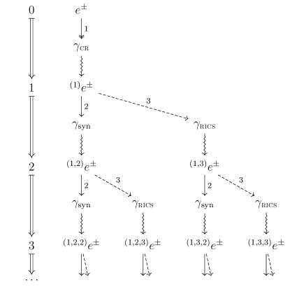
Figure 10: Diagram showing the general chain of physical processes in a strong polar cap cascade. Cascade generations are shown on the left – numbers connected by double arrows. Electrons and positrons $e^{\pm}$ produce photons which are turned into pairs of the next cascade generation: $\gamma_{\textrm{\scriptsize{{cr}}}}$ – via curvature radiation (solid line with double arrow labeled “1”), $\gamma_{\textrm{\scriptsize{syn}}}$ – via synchrotron radiation (solid lines with arrow labeled “2”), and $\gamma_{\textrm{\scriptsize{RICS}}}$ – via Resonant inverse Compton scattering (dashed lines with arrow labeled “3”). Numbers in parenthesis show the origin of each particle.

In Pap I we developed a simple semi-analytical cascade model which allowed us to simulate non-branching cascades – when only a single emission process is involved – and used it to explore CR-synchrotron cascades. As we argued in Pap I, such cascades develop in polar caps of moderately magnetized pulsars (B$\lesssim 10^{12}$G) where synchrotron radiation of secondary particles is the only source of photons creating pairs in the next cascade generation. In this paper we are interested in extending the range of applicability of our model for higher field pulsars as well as improving its accuracy. Our new model differs from the one in Pap I in two aspects (i) it applies to cascades with arbitrary emission/absorption processes – cascade branches can be arbitrarily complex and (ii) it can account for the fact that emission mechanisms can be broadband and not all emitted photons are able to create pairs.

6.1 General Algorithm

The spectral energy distribution of synchrotron and curvature radiation is broadband with a significant amount of energy emitted well below the peak energy $\epsilon_{\textrm{\scriptsize{peak}}}$

$$F(\epsilon)\propto\frac{\epsilon}{\epsilon_{\textrm{\scriptsize{peak}}}}\>\int_{0}^{\epsilon/\epsilon_{\textrm{\scriptsize{peak}}}}K_{5/3}(\zeta)\,d\zeta$$ (27)

where $K$ is the modified Bessel function of the order $5/3$. In Pap I we used a monoenergetic approximation for these processes – all energy is emitted as photons with energies $\epsilon_{\textrm{\scriptsize{peak}}}$. In our current model we divide the spectrum into 3 spectral bins $\{[0,0.3\epsilon_{\textrm{\scriptsize{peak}}}],[0.3\epsilon_{\textrm{\scriptsize{peak}}},1.5\epsilon_{\textrm{\scriptsize{peak}}}],[1.5\epsilon_{\textrm{\scriptsize{peak}}},\infty]\}$. CR and synchrotron emission of particles is modeled as emission of photons in each of the 3 spectral bins $j=1,2,3$ with energies

$$\epsilon^{j}\equiv{}f_{\epsilon}^{j}\>\epsilon_{\textrm{\scriptsize{peak}}}\,,$$ (28)

the number of photons emitted in each spectral bin is equal to the energy emitted by the particle in that bin $W^{i}=f_{w}^{i}\,W$ ($W$ is the total emission rate) divided by the characteristic energy of the photons

$$n^{j}=\frac{W^{j}}{\epsilon^{j}}=\frac{f_{w}^{j}}{f_{\epsilon}^{j}}\frac{W}{\epsilon_{\textrm{\scriptsize{peak}}}}\,.$$ (29)

Coefficients $(f_{\epsilon}^{j},f_{w}^{j})$ for energy bins we used are $\{(0.3,0.152)$, $(1,0.518)$, $(1.5,0.33)\}$; they are calculated by integrating spectral energy distribution $F(\epsilon)$, eq. (27), over the spectral bins.

In our algorithm both leptons and photons are macroparticles; the statistical weight of each particle is the number of real particles it represents. We start by calculating the energy of the primary particle accelerated in the gap according to §4 and follow this particle as it moves along magnetic field lines loosing energy emitting CR photons. Each CR photon initiates an electron-positron cascade with secondary particles emitting the next generation of pair producing photons via synchrotron radiation and Resonant Inverse Compton scattering (RICS) of soft X-ray photons from the NS surface. We follow every generation of photons until their energy falls below the escaping energy according to §3.3 and compute the number of pairs created by each cascade generation. The diagram in Fig. 10 shows the chain of physical processes initiated by a single CR photon. In Fig. 10, “rows” represent different cascade generations (particle with the same number of iterations particle/photon before their creation starting with primary particles), while “columns” correspond to branches (particles of the same generations produced by different emission processes). In each generation of the cascade, pairs $e^{\pm}$ produce photons which are then turned into pairs of the next generation: $\gamma_{\textrm{\scriptsize{{cr}}}}$ – via curvature radiation (shown by solid line with double arrow labeled “1”), $\gamma_{\textrm{\scriptsize{syn}}}$ – via synchrotron radiation (shown by solid lines with arrow labeled “2”), and $\gamma_{\textrm{\scriptsize{RICS}}}$ – via Resonant inverse Compton scattering (shown by dashed lines with arrow labeled “3”). Numbers in parenthesis show the origin of each particle, for example, (1,3,2) means that this pair was produced by synchrotron photon (2d generation) emitted by a pair produced by RICS photon (1st generation) created by CR photon (0th generation).

Our algorithm is described in detail in Appendix C; here we give its brief overview. The central part of our algorithm is the recursive function PairCreation(), Algorithm 2. For each photon PairCreation() calculates whether and where it will be absorbed to create a pair. The photon is counted as absorbed if its mfp is less than the escaping distance, $\lambda_{\gamma\rightarrow\pm}\leq s_{\textrm{\scriptsize{esc}}}R_{\textrm{\scriptsize{{ns}}}}$, and its absorption point $x$ is still inside the cascade zone, $x\leq s_{\textrm{\scriptsize{cascade}}}R_{\textrm{\scriptsize{{ns}}}}$. Then, for each emission process, it calculates the energy of the next generation photons emitted by the pair calling emission process specific function emissionFun(). And, finally, it recursively calls itself for each of the next generation photons. We follow the primary particle as it moves along magnetic field lines losing energy and emitting photons via curvature radiation – Algorithm 1 in Appendix C. For each CR photon PairCreation() is called and through its successive recursive calls follow every branch of the cascade. The total cascade multiplicity is calculated by integrating the number of particles produced in cascades generated by each CR photon (computed by recursive calls of PairCreation()) over the distance within the cascade zone. We assume that the size of the cascade zone is equal to the NS radius $R_{\textrm{\scriptsize{{ns}}}}$, $s_{\textrm{\scriptsize{cascade}}}=1$.

6.2 Microscopic processes

We analyzed the microphysics of polar cap cascades of young energetic pulsars in Pap I in great detail. Here we give a brief overview of how we treat the cascade microphysics.

At the distance $s$ after exiting the acceleration zone (hereafter all distances are normalized to $R_{\textrm{\scriptsize{{ns}}}}$) the energy of the primary particle is (eq. (19) in Pap I)

$$\epsilon_{\pm}(s)=\epsilon_{\pm}^{0}\left[1+3H\frac{(\epsilon_{\pm}^{0})^{3}}{\rho_{\textrm{\scriptsize{c}}}^{2}}s\right]^{-1/3}\,,$$ (30)

where $\epsilon_{\pm}^{0}$ is the initial particle energy, $H=(2/3)R_{\textrm{\scriptsize{{ns}}}}{}r_{e}\approx\mbox{$1.88\times 10^{-7}$}\mbox{cm}^{2}$, $r_{e}=e^{2}/m_{e}c^{2}$ is the classical electron radius. While traveling a segment of the length $ds$ the energy emitted by the primary particle via CR (all energy quantities are normalized to $m_{e}c^{2}$) is

$$W_{\textrm{\scriptsize{{cr}}}}=\frac{3}{2}\,\alpha_{f}\frac{\lambdabar{}_{\textrm{\scriptsize{{c}}}}R_{\textrm{\scriptsize{{ns}}}}}{\rho_{\textrm{\scriptsize{c}}}^{2}}\,\epsilon_{\pm}^{4}(s)\,ds$$ (31)

The peak energy of CR radiation photons is

$$\epsilon_{\textrm{\scriptsize{{CR}, peak}}}=\frac{3}{2}\frac{\lambdabar{}_{\textrm{\scriptsize{{c}}}}}{\rho_{\textrm{\scriptsize{c}}}}\epsilon_{\pm}{}^{3}$$ (32)

The energies and statistical weights of macroparticles representing CR photons are calculated from eq. (28), (29) using eqs. (31), (32)

We follow the evolution of cascades initiated by CR photons by tracing the pair producing photons as their energy degrades with each successive cascade generation. The energy of each pair-creating photon $\epsilon_{\gamma}$ is transferred to an electron-positron pair, which is always created with a non-zero perpendicular to the magnetic field momentum. The perpendicular energy is emitted by the pair via synchrotron radiation shortly after pair creation. The energy emitted as synchrotron photons is (see eq. (13) in Pap I)

$$W_{\textrm{\scriptsize{syn}}}=\epsilon_{\gamma}\left\{1-\left[1+\left(\frac{\chi_{a}}{b}\right)^{2}\right]^{-1/2}\right\}$$ (33)

and the peak energy of the synchrotron radiation is

$$\epsilon_{\textrm{\scriptsize{syn, peak}}}=\frac{3}{4}\chi_{a}\epsilon_{\gamma}\,,$$ (34)

where $\chi_{a}$ and $b$ are the value of the parameter $\chi_{a}$ and normalized magnetic field strength at the absorption point of the parent photon. As for CR, photons energies and statistical weights of macroparticles representing synchrotron photons are calculated from eq. (28), (29) using eqs. (33), (34).

Pair particles can also scatter thermal photons from the NS surface. If it happens in the cascade zone the kinetic energy associated with the motion of the particle parallel to the magnetic field is transferred to the next generation of pair producing photons. The maximum energy which can be emitted as RICS photons is the pair’s kinetic energy left after emission of synchrotron photons

$$W_{\textrm{\scriptsize{{rics}}}}^{0}=\epsilon_{\gamma}^{i-1}\left[1+\left(\frac{\chi_{a}}{b}\right)^{2}\right]^{-1/2}\,.$$ (35)

The mean free path for RICS is given by (Zhang & Harding, 2000; Sturner, 1995; Dermer, 1990):

$$\lambda_{\textrm{\scriptsize{{rics}}}} = -0.061\,\epsilon_{\pm}^{2}\,T_{6}^{-1}B_{12}^{-2}\times$$ (36)

$$\ln^{-1}\left[1-\exp\left(-\frac{134B_{12}}{\epsilon_{\pm}\,T_{6}(1-\mu_{s})}\right)\right]\,\mbox{cm}$$

where $T_{6}$ is the temperature of the NS surface in units of $10^{6}$K, $B_{12}$ is the magnetic field strength in units of $10^{12}$ G, and $\mu_{s}=\cos\theta_{s}$, where $\theta_{s}$ is the angle between the momenta of the scattering photon and particle in the lab frame. Eq. (36) implicitly takes into account the condition that soft photons must be in cyclotron resonance to be scattered, it is obtained by integration of the resonant cross-section with a blackbody spectrum of target photons (Dermer, 1990). If the mfp for RICS is larger than the size of the cascade zone, $\lambda_{\textrm{\scriptsize{RICS}}}>R_{\textrm{\scriptsize{{ns}}}}$, we assume that no RICS pair producing photons are emitted. As particles move away from the NS the probability of RICS decreases relative to that at the injection point due to the decrease on the magnetic field strength and the number density of soft photons. To account for this effect we assume that if $\lambda_{\textrm{\scriptsize{RICS}}}<0.1\,R_{\textrm{\scriptsize{{ns}}}}$ all pair’s kinetic energy left after emission of synchrotron photons is transferred to RICS photons, this fraction linearly decrease as $\lambda_{\textrm{\scriptsize{RICS}}}$ is getting bigger $\propto{}0.1R_{\textrm{\scriptsize{{ns}}}}/\lambda_{\textrm{\scriptsize{RICS}}}$, so that the energy emitted as RICS photons is

$$W_{\textrm{\scriptsize{{rics}}}}=\begin{cases}W_{\textrm{\scriptsize{{rics}}}}^{0},&\textrm{if }\lambda_{\textrm{\scriptsize{{rics}}}}\leq{}0.1\,R_{\textrm{\scriptsize{{ns}}}}\\ \frac{R_{\textrm{\scriptsize{{ns}}}}}{\lambda_{\textrm{\scriptsize{RICS}}}}\>W_{\textrm{\scriptsize{{rics}}}}^{0},&\textrm{if }0.1\,R_{\textrm{\scriptsize{{ns}}}}<\lambda_{\textrm{\scriptsize{{rics}}}}\leq R_{\textrm{\scriptsize{{ns}}}}\\ 0,&\textrm{if }\lambda_{\textrm{\scriptsize{{rics}}}}>R_{\textrm{\scriptsize{{ns}}}}\,.\\ \end{cases}$$ (37)

The spectrum of RICS radiation is narrow-band and we approximate this process as emission of monochromatic photons with the energy (see eq. (49) in Pap I)

$$\epsilon_{\gamma,\,\textrm{\scriptsize{{RICS}}}}=\epsilon_{\gamma}\,b\left[1+\left(\frac{\chi_{a}}{b}\right)^{2}\right]^{-1/2}\,.$$ (38)

This number of RICS photons emitted by each pair is

$$n_{\textrm{\scriptsize{{rics}}}}=\frac{W_{\textrm{\scriptsize{{rics}}}}}{\epsilon_{\gamma,\,\textrm{\scriptsize{{RICS}}}}}\,.$$ (39)

6.3 Model applicability

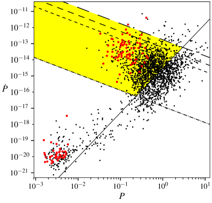
Figure 11: $P\dot{P}$ diagram with the yellow area showing the range of parameters where approximation for particle acceleration used in this paper is applicable, see text for description. Pulsars from ATNF catalog (Manchester et al. (2005), http://www.atnf.csiro.au/research/pulsar/psrcat) are shown by black dots, $\gamma$-ray pulsars from the second Fermi catalog (Abdo et al., 2013) by red dots.

The limitations of our model come from assumptions used in derivation of the energy of primary particles and the magnetic field strengths at which physical processes different from the ones we consider here become important. Eq. (19) for the energy of primary particles $\epsilon_{\pm,\,\textrm{\scriptsize{acc}}}$ was derived under the assumptions that (i) particles are accelerated freely, i.e. radiation reaction can be neglected and (ii) the length of the gap is much smaller that the polar cap radius, so that a one dimensional approximation can be used. We also do not model cascades for which photon splitting is important, so our model is applicable (iii) for magnetic field strength below $B_{\gamma\rightarrow\gamma\gamma}$, calculated according to eq. (14). Constraints (i), (ii), and (iii) together define the range of pulsar parameters where our cascade model is applicable. Constraints (i) and (ii) remain the same as in Pap I; they are derived in Appendixes B and C of Pap I correspondingly. Constraint (iii) – the magnetic field strength above which photon splitting becomes important for photons near the threshold of pair formation – depends on the radius of curvature of magnetic field lines $\rho_{\textrm{\scriptsize{c}}}$. In Fig. 11 we show the range of pulsar parameters for which our model is applicable superimposed on the $P\dot{P}$ diagram. The one-dimensional approximation (ii) is valid to the left of the solid line, the approximation (i) of free acceleration above the dot-dashed line (given by eq. 54 in Pap I). Pulsars with $B<B_{\gamma\rightarrow\gamma\gamma}$ are below the dashed lines. The line with short dashes correspond to $\rho_{\textrm{\scriptsize{c}}}=10^{6}$cm, $B_{\gamma\rightarrow\gamma\gamma}=\mbox{$4.4\times 10^{12}$}$G, the line with medium dashes – $\rho_{\textrm{\scriptsize{c}}}=10^{7}$cm, $B_{\gamma\rightarrow\gamma\gamma}=\mbox{$7.7\times 10^{12}$}$G, and the line with long dashes – $\rho_{\textrm{\scriptsize{c}}}=10^{8}$cm, $B_{\gamma\rightarrow\gamma\gamma}=\mbox{$1.3\times 10^{13}$}$. The yellow region shows the range of of pulsar periods and period derivatives where these three assumptions are valid. We see that most of young normal pulsars, including gamma-ray pulsars from the Fermi second pulsar catalog, fall in this range. Technically, the range of pulsar parameters for which our current model is applicable is only slightly different from that of Pap I (the limits on $B$ a less restrictive now, cf with Fig. 13 in Pap I), but our current model offers a considerably better treatment of cascades for $B\gtrsim 10^{12}$G.

7 Multiplicity of the full cascade

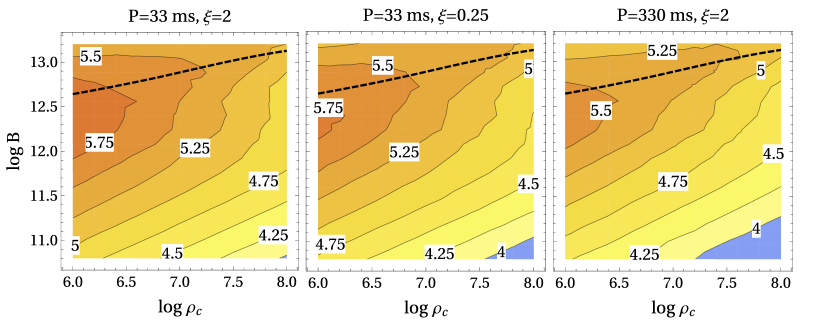
Figure 12: Multiplicity of polar cap cascades for different pulsar parameters $P$ and $\xi$. Contours of $\log\kappa$ as functions of logarithms of curvature of magnetic field lines $\rho_{\textrm{\scriptsize{c}}}$ in cm and magnetic field strength $B$ in Gauss for three sets of the gap parameters $(P[\mbox{ms}],\xi_{j})$: $(33,2)$, $(330,0.25)$, $(33,2)$. The temperature of NS surface was assumed to be $T=10^{6}$K. The critical magnetic field $B_{\gamma\rightarrow\gamma\gamma}$ above which photon splitting starts affecting cascade multiplicity is shown by the dashed line.

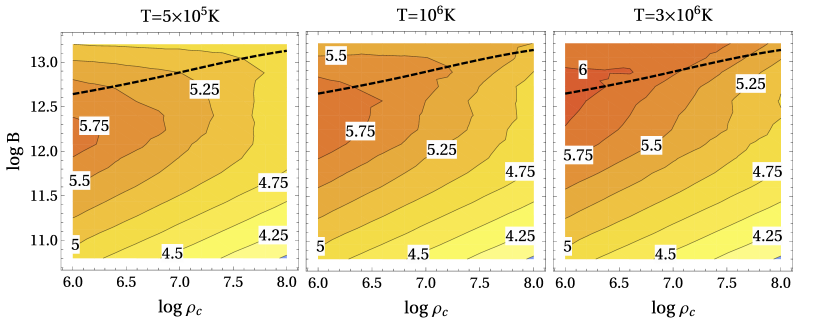
Figure 13: Multiplicity of polar cap cascades for different temperatures of the NS surface. Contours of $\log\kappa$ as functions of logarithms of curvature of magnetic field lines $\rho_{\textrm{\scriptsize{c}}}$ in cm and magnetic field strength $B$ in Gauss for three temperatures of NS surface $T=\mbox{$5\times 10^{5}$},10^{6},\mbox{$3\times 10^{6}$}$K. The pulsar parameters $P$ and $\xi$ are assumed to be $P=33$ms, $\xi=2$. The critical magnetic field $B_{\gamma\rightarrow\gamma\gamma}$ above which photon splitting starts affecting cascade multiplicity is shown by the dashed line. Note that the middle panel is the same as the left panel on Fig. 12.

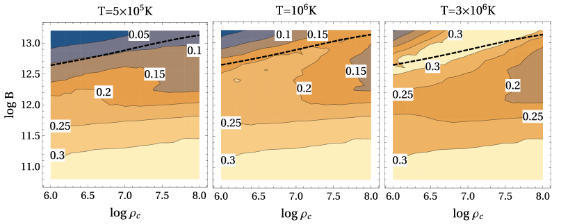
Figure 14: Efficiency of polar cap cascades $\kappa/\kappa_{\textrm{\scriptsize{max}}}$ for different temperatures of the NS surface. Contours of $\kappa/\kappa_{\textrm{\scriptsize{max}}}$ as functions of logarithms of curvature of magnetic field lines $\rho_{\textrm{\scriptsize{c}}}$ in cm and magnetic field strength $B$ in Gauss for cascade shown in Fig. 13.

For a wide range of pulsar parameters we computed maximum multiplicities of polar cap cascades with $\gamma{}B$ as the pair creation mechanism and CR, SR, and RICS of soft thermal photons from the NS surface as emission mechanisms according to the algorithm described in previous sections.

In Fig. 12 we show contours of cascade multiplicity $\log(\kappa)$ as a function of the magnetic field strength $\log(B)$ in Gauss and the radius of curvature of magnetic field lines $\log(\rho_{\textrm{\scriptsize{c}}})$ in cm for a NS with a uniform surface temperature of $T=10^{6}$ K. The dashed line indicates the parameter space above which photon splitting start (negatively) to affect the cascade multiplicity. The three plots in Fig. 12 are for different pulsar periods $P=33,330$ ms and two different filling factors $\xi=2,0.25$. The electric field in the gap for the case ($P=33$ ms, $\xi=2$) is an order of magnitude larger than in the other two cases, but the cascade multiplicity is only moderately higher, it is greater by less than $\sim 2$ times. Compared to the simple estimates from §5 the total multiplicity for the same pulsar parameters is smaller by the factor of $\sim 4-5$ – cf. Fig. 12 with Fig. 9 where $\kappa_{\textrm{\scriptsize{max}}}$ is plotted for the same combination of parameters. The maximum value for multiplicity reaches $6\times 10^{5}$ for smaller radii of curvature of magnetic field lines $\rho_{\textrm{\scriptsize{c}}}\sim 10^{6}$cm.

In the case of a pure CR-Synchrotron cascade discussed in Pap I (when the contribution of RICS is neglected), the cascade multiplicity is the highest for magnetic fields around $B\gtrsim 10^{12}$ G and drops for both higher and lower magnetic field strengths (Fig. 14 of Pap I). For cascades with RICS considered in this paper the multiplicity decrease for higher magnetic field, $B\gtrsim 10^{12}$ G, is much smaller, because the energy of pair parallel motion is returned back to the cascade by RICS. For lower magnetic field $B<10^{12}$G the differences in multiplicities between Fig. 12 and Fig. 14 of Pap I vary from a few percent for the case ($P=33$ ms, $\xi=2$) to $\sim 70\%$ for the case ($P=330$ ms, $\xi=2$). These differences are because of more accurate treatment of emission processes in this paper compared to Pap I.

In Fig. 13 we show plots illustrating the dependence of the cascade multiplicity on the NS surface temperature. Contours of $\log(\kappa)$ are plotted for three different temperatures of the NS surface $T=\mbox{$5\times 10^{5}$},10^{6},\mbox{$3\times 10^{6}$}$ K. The number of soft X-ray photons available for RICS changes dramatically with the temperature and so does the contribution of RICS to cascade multiplicity. For $T=\mbox{$5\times 10^{5}$}$ K the multiplicity profiles are very similar to those of CR-synchrotron cascades. For magnetic fields $B\gtrsim\mbox{$3\times 10^{12}$}$ G photons are absorbed after propagating a short distance and pairs are created with small perpendicular to $B$ momenta, which leaves a large fraction of the parent photon’s energy in the pairs’ parallel motion (this was discussed in detail in Pap I). If there are not enough soft X-ray photons to be up-scattered via RICS, this kinetic energy is lost from the cascade and the total multiplicity diminish. For higher surface temperatures the increasing number of soft photons makes RICS more and more efficient, which leads to the decrease of energy “leaks” from the cascade and the multiplicity $\kappa$ becomes similar to the maximum multiplicity $\kappa_{\textrm{\scriptsize{max}}}$. Indeed, for low temperature $T=\mbox{$5\times 10^{5}$}$K (left panel of Fig. 13) the plot for $\kappa$ is similar to $\kappa$ of CR-synchrotron cascade, and for high temperature $T=\mbox{$3\times 10^{6}$}$K (left panel of Fig. 13) the shape of $\kappa$ contours are similar to the ones of $\kappa_{\textrm{\scriptsize{max}}}$ shown on Fig. 9 (left panel).

The cascade efficiency $\kappa/\kappa_{\textrm{\scriptsize{max}}}$, which characterizes how the energy available to the cascade is converted into pairs, is shown in Fig. 14, for the same parameters as $\kappa$ on Fig. 13. For magnetic fields below $\lesssim 10^{12}$G the efficiency for all three surface temperatures is similar and $\gtrsim 20\%$; for these magnetic fields the RICS contribution is negligible and so the cascade behavior does not depend on the temperature. For stronger magnetic fields, the efficiency increases with the temperature. For high NS temperatures the cascade efficiency can be as large as 30%. We should note that because of photon splitting (which mostly affects RICS photons) the real cascade efficiency above the dashed lines is smaller than the values shown in Fig. 14.

To get a better understanding of polar cap cascades near their peak multiplicities we consider here several particular cascades and analyze their properties in detail. We consider cascades in polar caps of pulsar with $P=33$ ms, assume $\xi=2$ and use two values of the radius of curvature of magnetic field lines $\rho_{\textrm{\scriptsize{c}}}=10^{7}$ cm and $\rho_{\textrm{\scriptsize{c}}}=10^{7.9}\approx\mbox{$7.94\times 10^{7}$}$cm. For each value of $\rho_{\textrm{\scriptsize{c}}}$ we analyze cascade properties for three values of magnetic field strength to illustrate how the RICS contribution changes with $B$. These examples represent cascades near their highest multiplicities in polar caps of pulsars when (i) there is a significant non-dipolar component of the magnetic field ($\rho_{\textrm{\scriptsize{c}}}=10^{7}$cm) as well as (ii) pulsars with nearly unadulterated dipolar field ($\rho_{\textrm{\scriptsize{c}}}=10^{7.9}$cm). As we discussed earlier, the dependence of the cascade multiplicity on pulsar parameters is weak, so these examples should be representative for cascades in pulsars with a broad range of periods and filling factors $\xi$.

We visualize cascade development with three types of plots: (i) the cascade graphs (Figs. 15, 18), the cumulative pair injections rates decomposed according to (ii) emission mechanisms (Figs. 16, 19) and (iii) cascade generations (Figs. 17, 20). These plots show properties of the whole cascade, i.e. all pairs created by a single primary particle as it moves along magnetic field lines and emits CR photons which initiate multiple individual cascades. The cascade graphs in Figs. 15, 18 are the quantitative representations of the cascade diagram shown in Fig. 10. In these graphs vertices represents pairs with the same origin – the chain of emission processes which led to emission of these pairs’ parent photons is the same. The area of the circles at the graphs’ vertices is proportional to the number of pairs, however, their sizes are consistent only within the same graph, the sizes of the vertices of different graphs are not related. The cumulative pair injection rates $N(<x)$ for a given distance $x$, shown in Figs. 16, 17, 19, 20, are the total number of pairs created at distances less than $x$.

Polar cap cascades have 5-8 of generations at most. At each cascade generation pairs emit several photons which split the energy of the particle. This leads to rapid energy degradation through cascade generations and the cascade dies after several generations. On average, the most contribution comes from generation 4 (see Figs. 17, 20). The total multiplicity does not necessarily increase with the number of cascade branches – despite there being more branches and generations in case (d), the total multiplicity of these cascades is $\sim 2.5$ times lower than that of cascades for case (a).

Cases a-c and e-f represent cascades with the same values of $\rho_{\textrm{\scriptsize{c}}}$ ($10^{7}$cm and $10^{7.9}$cm correspondingly) and decreasing magnetic field strength. The role of RICS in cascades decreases with decreasing of $B$. For case (a) RICS is responsible for comparable, and for case (d) even slightly larger, number of pairs, see Figs. 16(a), 16(d). As a result cascades (a) and (d) have more branches that their counterparts with lower magnetic fields ((b), (c) and (e), (f) correspondingly), see Figs. 15, 18. RICS never becomes a dominating process, but it can contribute a comparable amount of pairs to the cascade as synchrotron radiation for high magnetic fields.

Another illustration of the fact that the number of cascade branches is not directly related to the total multiplicity is provided by comparison of cascades (d)-(f). The complexity of the cascades changes significantly (due to the diminishing role of RICS) but the total multiplicities of cascades (e), (f) are only $\sim 30\%$ and $55\%$ smaller than that of cascade (d). What matters most is the amount of energy available for the cascade, i.e. the relation of $\epsilon_{\pm,\,\textrm{\scriptsize{acc}}}$ and $\epsilon_{\gamma,\,\textrm{\scriptsize{esc}}}$, cf. Fig. 9.

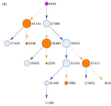
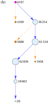
Figure 15: Cascade graphs for cascades in pulsars with $P=33$ms, $\xi=2$, $\rho_{\textrm{\scriptsize{c}}}=10^{7}$cm, $T=10^{6}$K, and the following magnetic field strengths: (a) $B=10^{12.5}$G, (b) $B=10^{12}$G, (c) $B=10^{11.5}$G. Each graph’s vertex represents pairs of the same origin – pairs produced in a certain cascade generation by photons emitted by pairs of the previous generation by the same emission mechanism. Lines connect vertices representing parent particles to the vertices representing child pairs with arrows directed towards the child pairs. Blue vertices and lines correspond to pairs created by synchrotron photons, orange vertices and dashed lines – to pairs created by RICS photons, and magenta vertices – to pairs created by CR photons. The size of each vertex (its area) is proportional to the total number of pairs, the numbers show the number of pairs represented by the vertices. The relative sizes of the vertices are consistent only within the same graph, sizes of vertices in different graphs are not related.

Figure 16: Cumulative pair injections rates $N(<x)$ for different emission mechanisms for cascades in pulsars with the same parameters as in Fig. 15. $N(<x)$ is the total number of pairs created at the distances less than the distance $x$. The total pair injection rate is shown by the black solid line. Dotted magenta line is the number of pairs created by CR photons, blue solid line – by synchrotron photons, dashed orange line – RICS photons. The total cascade multiplicity is shown in the upper left corner of each plot.

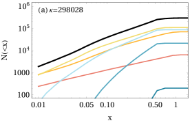
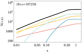
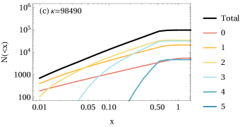
Figure 17: Cumulative pair injections rates $N(<x)$ for different cascade generations for cascades in pulsars with the same parameters as in Fig. 15. The total pair injection rate is shown by the black solid line. Pair injection rates for different cascade generations are shown by color lines according to the legend to the right of the panel (c).

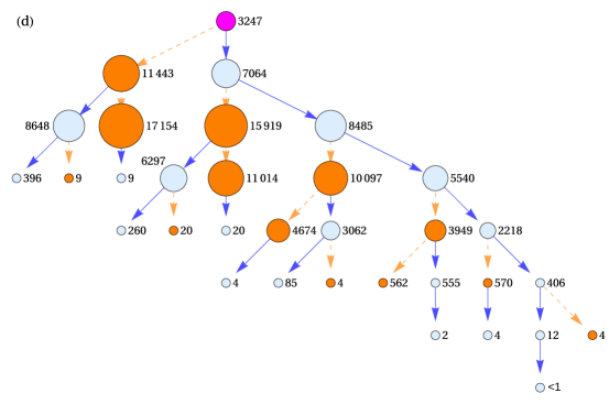
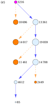
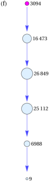
Figure 18: Cascade graphs for cascades in pulsars with $P=33$ms, $\xi=2$, $\rho_{\textrm{\scriptsize{c}}}=10^{7.9}\approx\mbox{$7.94\times 10^{7}$}$cm and the following magnetic field strengths: (d) $B=10^{12.9}$G, (e) $B=10^{12.5}$G, (f) $B=10^{12}$G. Notations are the same as in Fig. 15.

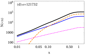
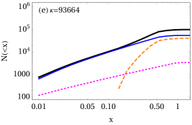
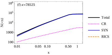
Figure 19: Cumulative pair injections rates $N(<x)$ for different emission mechanisms for cascades in pulsars with the same parameters as in Fig. 18. Notations are the same as in Fig. 16

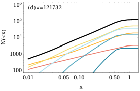
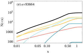
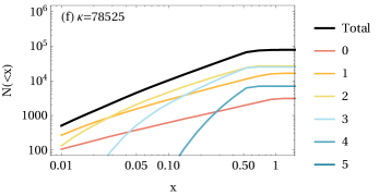
Figure 20: Cumulative pair injections rates $N(<x)$ for different cascade generations for cascades in pulsars with the same parameters as in Fig. 15. Notations are the same as in Fig. 17

We used different values for the photon escape distance $s_{\textrm{\scriptsize{esc}}}=0.5$ and the size of the cascade zone $s_{\textrm{\scriptsize{cascade}}}=1$. The value of $s_{\textrm{\scriptsize{esc}}}$ has a direct impact on the energy of escaping photons according to eq. (15), and the multiplicity dependence is close to $\propto{}1/s_{\textrm{\scriptsize{esc}}}$. On the other hand, the exact value of $s_{\textrm{\scriptsize{cascade}}}$, which limits the range where photons can be emitted and absorbed, has little impact on the total multiplicity as long as $s_{\textrm{\scriptsize{cascade}}}\geq s_{\textrm{\scriptsize{esc}}}$. As is evident from Figs. 17,20 most pairs are produces at distances $<s_{\textrm{\scriptsize{esc}}}$ from the NS which implies that their parent photons are emitted at distances a few time smaller than $s_{\textrm{\scriptsize{cascade}}}$. The contribution from photons emitted at distances approaching $s_{\textrm{\scriptsize{cascade}}}$ is rather small – primary particles have lost a large fraction of their energy and resulting cascades have only 1-2 generations.

Synchrotron photons have mostly $\perp$ polarization and RICS $\parallel$ one. The photons susceptible to splitting are the ones with $\perp$ polarization. At the field strength where photon splitting becomes important RICS photons provide a comparable of larger number of pairs, hence the splitting should significantly affect cascade multiplicity. The highest cascade multiplicity is reached for $B$ and $\rho_{\textrm{\scriptsize{c}}}$ values near the dashed lines in Figs. 12, 13. So, the pulsars with highest multiplicities should have $B\sim\mbox{$4.4\times 10^{12}$}-\mbox{$1.4\times 10^{13}$}$G, depending on $\rho_{\textrm{\scriptsize{c}}}$, and surface temperature $T\gtrsim 10^{6}$ K. On the $P\dot{P}$ diagram, Fig. 11, the pulsars with the highest maximum multiplicity are those near the dashed lines.

The spatial distribution of pair injection rate shows that most of the pairs produced by RICS photons are created at distances comparable to $R_{\textrm{\scriptsize{{ns}}}}$, which are much larger than the polar cap size $r_{\textrm{\scriptsize{pc}}}\approx\mbox{$1.45\times 10^{4}$}P^{-1/2}$cm. If soft X-ray photons are emitted from the whole surface of the NS, as assumed in our model, their number density does not decrease dramatically throughout the cascade zone. However, if soft photons are emitted from a hot polar cap, and the rest of the NS surface is cold, $T<10^{6}$K, the number density of soft photons at distances $\gg r_{\textrm{\scriptsize{pc}}}$ will be much smaller than assumed here. In that case the role of RICS is reduced and the polar cap cascade will operate in the CR-synchrotron regime. In the latter case the multiplicity will reach its peak at $B\sim 10^{12}$G (for detailed analysis of CR-synchrotron cascades see Pap I).

8 Discussion

In our previous paper, Pap I, we limited ourselves to CR-synchrotron cascades, which was an adequate approximation for most young energetic pulsars. However right where CR-synchrotron cascades reach their highest multiplicity, RICS becomes an important emission mechanism and in order to get an accurate limit on the maximum cascade multiplicity it must be taken into account. In this study we included in our model all three processes leading to emission of pair producing photons in polar caps of energetic pulsars – RICS, synchrotron and curvature radiation – and considered the effect on photon splitting on the cascade multiplicity. The treatment of the radiation is improved, dividing the spectrum into three energy bands instead of the delta-function approximation used in Pap I. We used a more accurate prescription for the single photon pair production which takes into account the decrease of the attenuation coefficient near the pair formation threshold – an important correction for pair formation in magnetic fields with $B\gtrsim 10^{12}$G. We also used a more consistent treatment of the particle acceleration by finding both the energy and the primary particles $\epsilon_{\pm,\,\textrm{\scriptsize{acc}}}$ and parameter $\chi_{a,\,\textrm{\scriptsize{acc}}}$, which regulates pair injection and termination of acceleration zone, simultaneously. We developed a new semi-analytical algorithm which can incorporate an arbitrary number of microphysical processes, model cascades spatial evolution, and allow fast exploration of cascades parameter space. The improvements upon the model presented in Pap I allowed us to conduct a reasonably accurate study of polar cap cascades in the regime where they reach their highest multiplicity. Our current model includes the most important microphysical processes relevant for polar cap cascades in young energetic pulsars with the highest pair yield.

The goal of our study was to find the upper limit on the multiplicity of electron positron cascades in pulsars. We have performed a systematic study of pair cascades above pulsar polar caps for a variety of input parameters including surface magnetic field, pulsar rotation period, primary particle energy, magnetic field radius of curvature, and the temperature of NS surface. We used the modern description for particle acceleration derived from self-consistent models of the polar cap acceleration zone, i.e. those that are capable of generating currents consistent with global models of the pulsar magnetosphere. In our model we do not address directly the non-stationary nature of pulsar cascades. We considered pair cascades generated by primary particles accelerated at the peak of the pair formation burst. The intermittency of the pair formation process reduces the total pair yield and by studying cascades generated by the most energetic primary particles we achieved our goal of finding the limit on pair cascade multiplicity.

We find that pair multiplicity is maximized for pulsars with hot $T\geq 10^{6}$K surfaces. These must be very young pulsars which have not yet cooled down. For such pulsars, cascade multiplicity (almost) monotonically grows with increasing $B$ and decreasing $\rho_{\textrm{\scriptsize{c}}}$ until photon splitting becomes more important than pair production, which happens first in the last cascade generation. In young hot pulsars, pair cascades reach their highest multiplicities near magnetic field strengths where photon splitting becomes more efficient than single photon pair production for the last generation pair-producing photons. The maximum multiplicity is in the range $\kappa\sim 10^{6}-\mbox{$3\times 10^{5}$}$ for magnetic field strengths $\mbox{$3\times 10^{12}$}\mbox{G}\lesssim{}\,B\,\lesssim{}10^{13}\mbox{G}$ depending on the radius of curvature of magnetic field lines – the low and upper limits are for $\rho=10^{6}$cm and $10^{8}$cm correspondingly. For older pulsars, whose surfaces have cooled down below $10^{6}$K, the maximum cascade multiplicity is in the range $\kappa\sim\mbox{$5\times 10^{5}$}-10^{5}$ and it is achieved at $B\sim{}10^{12}$G. Even if old pulsars have hot polar caps, the density of soft photons at distances comparable to the NS radius will be too small to sustain efficient RICS and so the cascade operates in the CR-synchrotron regime even for high magnetic field strengths.

Here we ignored geometrical effects caused by curvature of magnetic field lines. For the smallest values of $\rho_{\textrm{\scriptsize{c}}}{}$, magnetic field line at large distances from the NS within the cascade zone can bend rather significantly. Such bending causes the displacement of particles in the lateral direction which, however, would have a negligible effect on the cascade multiplicity in pulsars with hot surfaces because it does not affect CR and synchrotron radiation and the variation of the incident angle of incoming thermal photons is washed out by the large solid angle these photons are coming from. It would only affect the lateral spreading of the cascade. In long period pulsars, where the NS surface is cold and the only source of the soft X-rays is the hot polar cap the effects of field line bending might potentially increase the multiplicity of the cascade. The pairs’ momenta in that case would have larger angle with soft photons what could increase the cross-section to photon scattering. However, the efficiency of RICS as an emission process is based in part on the wide range of angles thermal photons are coming from. Due to the large range of photon incident angles, pairs within a wide range of energies can still scatter thermal photons (with relatively narrow energy distribution) in the resonant regime – pairs of different energies scatter photons coming from different directions (Dermer, 1990). In the case of hot polar caps, the range of photon incident angles will be small (e.g. compared to the case of the hot NS surface), and the potential increase of scattering cross-section could benefit pairs of a single generation at best, thus making this effect of little importance.

The multiplicity at the peak of the cascade cycle is not very sensitive to the pulsar period, magnetic field and radius of curvature of the magnetic field lines. The multiplicity varies by less than $\sim$ an order of magnitude for the range of pulsar parameters spanning two or more orders of magnitude. The reason for this is self-regulation of the accelerator by pair creation: for pulsar parameters resulting in more efficient pair production, the size of the acceleration gap is smaller and the primary particle energy is lower and vice-versa.

Even the most efficient cascades typically have only several generations. High multiplicity is achieved because particles of each generations emit multiple pair producing photons. The biggest contribution comes from individual cascades with 3-4 generations. RICS can play an important role in polar caps cascades; it can provide an even larger number of pairs than synchrotron radiation, but synchrotron radiation never becomes a negligible process. When RICS is an important process the cascade can have many branches, but the multiplicity does not directly depend on cascade complexity (number of branches and generations). A more important factor is the energy available for the cascade process; the exact way of how this energy is distributed among the final pair population, i.e. via synchrotron or RICS branches, plays a secondary role.

The main factor determining the total yield of polar cap cascades is, however, the variation of the flux of primary particles due to intermittency of the particle acceleration in time-dependent cascades. Simple estimates for the “duty cycle” of the particle acceleration, presented in §10 of Pap I, predict that the total pair yield of polar cap cascade will be lower than the multiplicity values of cascades at the peak of the pair formation burst by a factor ranging from a $\sim$few for the case of space charge-limited flow (free particle extraction from the NS) with super Goldreich-Julian current density ($j/j_{\textrm{\scriptsize{{gj}}}}>1$) and up to $\sim$several hundred for the case of Ruderman-Sutherland gaps (no particle extraction from the PC) and space charge-limited flow with anti Goldreich-Julian current density ($j/j_{\textrm{\scriptsize{{gj}}}}<0$). The effective pair multiplicity then can not exceed a $\sim\mbox{$\mbox{few}\times 10^{5}$}$ even under the most favorable conditions – in young hot pulsars with high magnetic field $B\sim\mbox{$3\times 10^{12}$}$G and a significant non-dipolar component of the magnetic field in polar caps so that $\rho_{\textrm{\scriptsize{c}}}\lesssim{}10^{7}$cm.

An accurate estimate of the duty cycle requires self-consistent modeling of particle acceleration with much higher numerical resolution than was done in Timokhin & Arons (2013); Timokhin (2010), which will be a subject of a future paper. The results of this paper can then be easily adopted into a consistent model of pair supply in pulsars by scaling the multiplicity values obtained here by the duty cycle of particle acceleration. The semi-analytical model presented here can also guide more accurate (and time consuming) numerical simulations of cascades.

In terms of the direct astrophysical implication of this work, our main message is simple – under no circumstances can the pair yield of pulsars be greater than $\sim\mbox{$\mbox{several}\times 10^{5}$}n_{\textrm{\scriptsize{{gj}}}}$. This should be taken into account for examples in modeling of PWNe and lepton components of cosmic rays.

Appendix A Non-resonant inverse Compton scattering in pulsar polar cap cascades

Pairs can scatter soft X-ray photons emitted by the NS surface in resonant as well as non-resonant regime. However, as we show below, the non-resonant Inverse Compton Scattering (ICS) is a very inefficient emission mechanism and can be neglected in comparison with scattering in resonant regime.

An emission process could play a role in polar cap cascades if the distance over which a particle looses a substantial part of its energy to that emission process is less that the size of the cascade zone, which in this work is assumed to be $R_{\textrm{\scriptsize{{ns}}}}$. In Fig. 21 we plot contours of the mfp $\lambda_{\textrm{\scriptsize{NRICS}}}$ (in cm) of an electron/positron to Non-Resonant Inverse Compton Scattering (NRICS) of soft photons emitted by the NS surface as a function of the particle’s energy and the temperature of the NS. The mfp was calculated by integrating the full ICS cross-section over the non-isotropic distribution of photons emitted by the NS surface, photons are coming in the solid angle which is centered around particle’s momentum and limited by $(0\leq\theta<\theta_{\max};0\leq\phi\leq{}2\pi)$, with $\cos\theta_{\max}=0.5$ (in this paper we use the same solid angle for modeling RICS). The spectral energy distribution of thermal photons was modeled as the Rayleigh-Jeans power law with the high energy cut-off chosen in such a way that the total emitted energy is consistent with the Stefan-Boltzmann law It is easy to see from that plot that the mfp to NRICS becomes less that the NS radius only for very high temperatures of the NS surface, $T\gtrsim\mbox{$2\times 10^{6}$}$K, and even for $T\gtrsim\mbox{$3\times 10^{6}$}$K the mfp is only $\lambda_{\textrm{\scriptsize{NRICS}}}\simeq 0.2\,R_{\textrm{\scriptsize{{ns}}}}$. According to common models of NS cooling even the youngest pulsars should have surface temperatures less that $3\times 10^{6}$K (e.g. Haensel et al., 2007). This implies that it highly unlikely that in polar caps of pulsars particles could loose any significant fraction of their energy to non-resonant ICS.

But even if the NS surface is very hot, at the upper limit of the predicted temperature range, $T\simeq\mbox{$3\times 10^{6}$}$K, NRICS would be still of very limited relevance for cascade physics. The reason is as follows. From Fig. 21 it is clear that NRICS might be relevant for particles with energies $10^{3}\lesssim{}\epsilon_{\pm}\lesssim{}10^{4}$. Let us compare now the efficiency of resonant and non-resonant ICS. In Fig. 22 we plot contours of the logarithm of the ratio of the mean free paths of a particle to non-resonant and resonant ICS $\lambda_{\textrm{\scriptsize{NRICS}}}/\lambda_{\textrm{\scriptsize{RICS}}}$ as a function of particle energy and the strength of the magnetic field for the surface temperature $T=\mbox{$3.5\times 10^{6}$}$K. In the energy range $10^{3}\lesssim{}\epsilon_{\pm}\lesssim{}10^{4}$, where a significant part of particle’s momentum could be radiated via NRICS within the cascade zone, $\lambda_{\textrm{\scriptsize{NRICS}}}$ is less that $\lambda_{\textrm{\scriptsize{RICS}}}$ only for magnetic fields $B\lesssim\mbox{$3\times 10^{12}$}$G. For magnetic field strengths $\lesssim 10^{12}$G the fraction of the parent photon’s energy going into the parallel momentum of the created pair is smaller than $\sim{}30\%$ – most of the energy is emitted as synchrotron photons, see Pap I, Section 4, Fig. (5). In the narrow range of magnetic field strengths $10^{12}\mbox{G}\lesssim{}B\lesssim\mbox{$3\times 10^{12}$}$G NRICS might become an important process, but only for particles of a single cascade generation. Indeed, because of a very steep dependence of $\lambda_{\textrm{\scriptsize{NRICS}}}/\lambda_{\textrm{\scriptsize{RICS}}}$ on particle energy for a given value of $B$, even if pairs of some generation with the energy in the range $10^{3}\lesssim{}\epsilon_{\pm}\lesssim{}10^{4}$ do create photons more efficiently in the non-resonant regime, the next generation of pairs will scatter photons more efficient in the resonant regime.

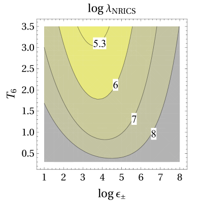
Figure 21: Contour plot of the logarithm of the mean free path of a particle to non-resonant ICS $\lambda_{\textrm{\scriptsize{NRICS}}}$ (in cm) as a function of the logarithm of the particle energy $\epsilon_{\pm}$ and the temperature of the NS surface $T_{6}$ (in units of $10^{6}$K).

Figure 22: Contour plot of the logarithm of the ratio of mean free paths of a particle to non-resonant and resonant ICS $\lambda_{\textrm{\scriptsize{NRICS}}}/\lambda_{\textrm{\scriptsize{RICS}}}$ as a function of the logarithm of the particle energy $\epsilon_{\pm}$ and the logarithms of the magnetic field strength $B$ in Gauss.

Appendix B Optical depths for single photon pair creation in ultrastrong magnetic field

In Pap I we adopted the widely used Erber (1966) formula for the opacity for single photon pair production in a strong magnetic field

$$\alpha_{\gamma\rightarrow\pm}(\epsilon_{\gamma},\psi)=0.23\,\frac{\alpha_{f}}{\lambdabar{}_{\textrm{\scriptsize{{c}}}}}\>b\,\sin\psi\,\exp\left(-\frac{4}{3\chi}\right)$$ (B1)

where $b\equiv{}B/B_{q}$ is the local magnetic field strength $B$ normalized to the critical quantum magnetic field $B_{q}=e/\alpha_{f}\lambdabar{}_{\textrm{\scriptsize{{c}}}}^{2}=\mbox{$4.41\times 10^{13}$}$ G, $\psi$ is the angle between the photon momentum and the local magnetic field, $\alpha_{f}=e^{2}/\hbar{}c\approx{}1/137$ is the fine structure constant, and $\lambdabar{}_{\textrm{\scriptsize{{c}}}}=\hbar/mc=\mbox{$3.86\times 10^{-11}$}$ cm is the reduced Compton wavelength. The parameter $\chi$ is defined as

$$\chi\equiv\frac{1}{2}\,\epsilon_{\gamma}b\,\sin\psi\,,$$ (B2)

where $\epsilon_{\gamma}$ is the photon energy in units of $m_{e}c^{2}$. Expression (B1) has been obtained in the asymptotic limit of $\chi\ll{}1$ and $b\ll{}1$. While $\chi\ll{}1$ is a good approximation for gamma-rays absorbed in polar caps in all pulsars (see §3.1), the approximation $b\ll{}1$ can become too restrictive for pulsars with higher magnetic fields. For pairs created near the kinematic threshold

$$\epsilon_{\gamma}\sin\psi=2$$ (B3)

eq. (B1) can overestimate the opacity by a factor of a few for pulsars with magnetic fields $\gtrsim\mbox{$3\times 10^{12}$}$G (Daugherty & Harding, 1983). The discrepancy becomes larger for stronger fields. An accurate treatment of the pair creation cross-section for non-small $b$ and/or near-threshold pair creation requires summation over a finite number of cyclotron energy levels of created pairs which results in unwieldy expressions (like eq. 6 in Daugherty & Harding (1983)). For our semi-analytical model such treatment would be an overkill, resulting in unnecessary complication of the model. Instead we use the numerical fit to the exact expression for the opacity suggested by Daugherty & Harding (1983) (their eq. 24)

$$\alpha_{\gamma\rightarrow\pm}(\epsilon_{\gamma},\psi)=\begin{cases}\displaystyle 0.23\,\frac{\alpha_{f}}{\lambdabar{}_{\textrm{\scriptsize{{c}}}}}\>b\,\sin\psi\,\exp\left(-\frac{4f_{\alpha}(\epsilon_{\gamma},b)}{3\chi}\right),&\text{ if }\epsilon_{\gamma}\sin\psi\geq 2\\ 0,&\text{ if }\epsilon_{\gamma}\sin\psi<2\end{cases}$$ (B4)

where

$$f_{\alpha}=1+0.42\,\left(\frac{1}{2}\>\epsilon_{\gamma}\sin\psi\right)^{-2.7}b^{-0.0038}\,.$$ (B5)

The second term in $f_{\alpha}$ is significant only for pair creation close to the threshold (B3). The non-zero part of expression (B4) for $\alpha_{\gamma\rightarrow\pm}$ can be written as

$$\alpha_{\gamma\rightarrow\pm}(\epsilon_{\gamma},\psi)=0.23\,\frac{\alpha_{f}}{\lambdabar{}_{\textrm{\scriptsize{{c}}}}}\>b\,\sin\psi\,\exp\left(-\frac{4}{3\chi}\right)\exp\left(-0.56\,\frac{b^{2.6962}}{\chi^{3.7}}\right)\,,$$ (B6)

i.e. it differs from the usual Erber’s formula (B1) by the exponential term

$$f_{\alpha,1}(b,\chi)\equiv\exp\left(-0.56\,\frac{b^{2.6962}}{\chi^{3.7}}\right)\,.$$ (B7)

This term significantly differs from 1 when pair formation occurs close to threshold.

The optical depths for pair creation by a photon in a strong magnetic field after propagating a distance $l$ is

$$\tau(\epsilon_{\gamma},l)=\int_{0}^{l}\alpha_{\gamma\rightarrow\pm}(\epsilon_{\gamma},\psi(x))\,dx\,,$$ (B8)

where integration is along the photon’s trajectory. For photons emitted tangent to the magnetic field line, $dx=\rho_{\textrm{\scriptsize{c}}}d\psi$, where $\rho_{\textrm{\scriptsize{c}}}$ is the radius of curvature of magnetic field lines; the angle $\psi$ is always small so the approximation $\sin\psi\approx\psi$ is very accurate. In our approximation of constant magnetic field both $b$ and $\rho_{\textrm{\scriptsize{c}}}$ are constants. From eq. (B2) we have $\psi=2\chi/\epsilon_{\gamma}{}b$, and substituting it into eq. (B8) we can express the optical depth $\tau$ to pair production as an integral over $\chi$

$$\tau(\epsilon_{\gamma},l)=A_{\tau}\,\frac{\rho_{\textrm{\scriptsize{c}}}}{\epsilon_{\gamma}^{2}b}\;\int_{0}^{\chi(\epsilon_{\gamma},\psi(l))}\chi\exp\left(-\frac{4}{3\chi}\right)\,f_{\alpha,1}(b,\chi)\>d\chi\,,$$ (B9)

where $A_{\tau}\equiv{}0.92\alpha_{f}/\lambdabar{}_{\textrm{\scriptsize{{c}}}}\approx\mbox{$1.74\times 10^{8}$}\;\mbox{cm}^{-1}$. If we expand the term $f_{\alpha,1}$ in a Taylor series the integral in eq. (B9) can be represented as a sum of integrals $\int x^{\xi}\exp(-x)\,dx$; each of those integrals can be integrated analytically.

We expand $f_{\alpha,1}$ in a Taylor series as $e^{-x}\approx{}1-x+x^{2}/2-\dots$ and keep up to the $5^{\text{th}}$ term

$$f_{\alpha,1}(b,\chi)\approx{} 1-0.56\>\frac{b^{2.6962}}{\chi^{3.7}}+0.1568\>\frac{b^{5.3924}}{\chi^{7.4}}-0.02927\>\frac{b^{8.0886}}{\chi^{11.1}}$$ (B10)

$${}+\mbox{$4.0977\times 10^{-3}$}\>\frac{b^{10.7848}}{\chi^{14.8}}-\mbox{$4.5894\times 10^{-4}$}\>\frac{b^{13.481}}{\chi^{18.5}}\,.$$

Only odd order term expansions are monotonic and we find that $3^{\text{rd}}$ order series is not a good enough approximation near the threshold. Eq. (B10) provides a good fit with the minimum number of terms – see Fig. 23.

Figure 23: Fifth order Taylor series expansion for $f_{\alpha,1}$ given by eq. (B10) – dashed lines – compared to the value given by eq. (B7) – solid lines – as a function of $\chi$ for 5 values of the magnetic field $b=0.01,0.11,0.21,0.31,0.41$ (lines from left to right).

Substituting expansion (B10) into eq. (B9) we get an analytical expression for the optical depth as a series of special functions

$$\tau(\chi)=A_{\tau}\,\frac{\rho_{\textrm{\scriptsize{c}}}}{\epsilon_{\gamma}^{2}b}\;\left[\frac{16}{9}\>\Gamma\left(-2,\frac{4}{3\chi}\right)-0.3434\>b^{2.6962}\,\Gamma\left(1.7,\frac{4}{3\chi}\right)\right.\\ +\mbox{$3.3165\times 10^{-2}$}\>b^{5.3924}\,\Gamma\left(5.4,\frac{4}{3\chi}\right)-\mbox{$2.1354\times 10^{-3}$}\>b^{8.0886}\,\Gamma\left(9.1,\frac{4}{3\chi}\right)\\ \left.+\mbox{$1.0312\times 10^{-4}$}\>b^{10.7848}\,\Gamma\left(12.8,\frac{4}{3\chi}\right)-\mbox{$3.9835\times 10^{-6}$}\>b^{13.481}\,\Gamma\left(16.5,\frac{4}{3\chi}\right)\right]\,.$$ (B11)

The special function $\Gamma(a,x)$ is the so-called upper incomplete gamma function, defined as $\Gamma(a,x)=\int_{x}^{\infty}t^{a-1}\exp(-t)\,dt$. There are efficient numerical algorithms for its calculation implemented in numerical libraries and scientific software tools; using eq. (B11) for calculation of the optical depths result in more efficient numerical codes than direct integration of eq. (B9).

For $b\ll 1$, when the opacity is given by the Erber’s formula (B1), the optical depths to pair creation is given by the first term in eq. (B11)

$$\tau(\chi)=\frac{16}{9}A_{\tau}\,\frac{\rho_{\textrm{\scriptsize{c}}}}{\epsilon_{\gamma}^{2}b}\;\Gamma\left(-2,\frac{4}{3\chi}\right)\,.$$ (B12)

This expression is a more compact from of the expression for $\tau(\chi)$ from Pap I(eq. 6 in that paper) as

$$\frac{16}{9}\>\Gamma\left(-2,\frac{4}{3\chi}\right)=\left[\frac{\chi^{2}}{2}\left(1-\frac{4}{3\chi}\right)e^{-\frac{4}{3\chi}}-\frac{8}{9}\,\mbox{Ei}\left(-\frac{4}{3\chi}\right)\right]\,.$$

For $\chi\ll 1$ eq. (B12) can be simplified further by expanding it into Taylor series around $\chi=0$ and retaining the first term

$$\tau(\chi)=\frac{3}{4}A_{\tau}\,\frac{\rho_{\textrm{\scriptsize{c}}}}{\epsilon_{\gamma}^{2}b}\;\chi^{3}e^{-\frac{4}{3\chi}}\,.$$ (B13)

Appendix C Algorithms for semi-analytical calculation of cascade multiplicity

$$\begin{array}[]{cc}&\textrm{\scriptsize{}Emission Process ID /Name/}\\ \rotatebox[origin={c}]{90.0}{\scriptsize{Cascade Generation}}&\hbox{}\vbox{\kern 15.00002pt\hbox{$\kern 0.0pt\kern 15.00002pt\kern-5.0pt\left[\kern 0.0pt\kern-15.00002pt\kern-5.55557pt\vbox{\kern-15.00002pt\vbox{\vbox{ \halign{\kern\arraycolsep\hfil\@arstrut$\kbcolstyle#$\hfil\kern\arraycolsep& \kern\arraycolsep\hfil$\@kbrowstyle#$\ifkbalignright\relax\else\hfil\fi\kern\arraycolsep&& \kern\arraycolsep\hfil$\@kbrowstyle#$\ifkbalignright\relax\else\hfil\fi\kern\arraycolsep\cr 5.0pt\hfil\@arstrut$\scriptstyle{}$\hfil\kern 5.0pt&5.0pt\hfil$\scriptstyle 0\;\textrm{/CR/}$\hfil\kern 5.0pt&5.0pt\hfil$\scriptstyle 1\;\textrm{/Syn/}$\hfil\kern 5.0pt&5.0pt\hfil$\scriptstyle 2\;\textrm{/RICS/}\\0$\hfil\kern 5.0pt&5.0pt\hfil$\scriptstyle\left\{(0):\left<\kappa_{0},\dots,\kappa_{nx}\right>\right\}$\hfil\kern 5.0pt&5.0pt\hfil$\scriptstyle 0$\hfil\kern 5.0pt&5.0pt\hfil$\scriptstyle 0\vskip 6.0pt plus 2.0pt minus 2.0pt\\1$\hfil\kern 5.0pt&5.0pt\hfil$\scriptstyle 0$\hfil\kern 5.0pt&5.0pt\hfil$\scriptstyle\left\{(0,1):\left<\kappa_{0},\dots,\kappa_{nx}\right>\right\}$\hfil\kern 5.0pt&5.0pt\hfil$\scriptstyle\left\{(0,2):\left<\kappa_{0},\dots,\kappa_{nx}\right>\right\}\vskip 6.0pt plus 2.0pt minus 2.0pt\\2$\hfil\kern 5.0pt&5.0pt\hfil$\scriptstyle 0$\hfil\kern 5.0pt&5.0pt\hfil$\scriptstyle\begin{Bmatrix}(0,1,1):\left<\kappa_{0},\dots,\kappa_{nx}\right>\\ (0,2,1):\left<\kappa_{0},\dots,\kappa_{nx}\right>\end{Bmatrix}$\hfil\kern 5.0pt&5.0pt\hfil$\scriptstyle\begin{Bmatrix}(0,2,2):\left<\kappa_{0},\dots,\kappa_{nx}\right>\\ (0,1,2):\left<\kappa_{0},\dots,\kappa_{nx}\right>\end{Bmatrix}\vskip 6.0pt plus 2.0pt minus 2.0pt\\\vdots$\hfil\kern 5.0pt&5.0pt\hfil$\scriptstyle\vdots$\hfil\kern 5.0pt&5.0pt\hfil$\scriptstyle\vdots$\hfil\kern 5.0pt&5.0pt\hfil$\scriptstyle\vdots\vskip 6.0pt plus 2.0pt minus 2.0pt\\n$\hfil\kern 5.0pt&5.0pt\hfil$\scriptstyle 0$\hfil\kern 5.0pt&5.0pt\hfil$\scriptstyle\begin{Bmatrix}(\texttt{orgn}_{1}):\left<\kappa_{0},\dots,\kappa_{nx}\right>\\ (\texttt{orgn}_{2}):\left<\kappa_{0},\dots,\kappa_{nx}\right>\\ \vdots\end{Bmatrix}$\hfil\kern 5.0pt&5.0pt\hfil$\scriptstyle\begin{Bmatrix}(\texttt{orgn}_{1}):\left<\kappa_{0},\dots,\kappa_{nx}\right>\\ (\texttt{orgn}_{2}):\left<\kappa_{0},\dots,\kappa_{nx}\right>\\ \vdots\end{Bmatrix}\\$\hfil\kern 5.0pt\crcr}}}}\right]$}}\end{array}$$

Figure 24: Structure of the cascade matrix. Each row contains information about pairs created in the generation which number is equal to the row number. Each column contains information about pairs created by photons emitted by the emission process id which is equal to the column number; in this case the IDs of the emission processes are: 0-CR, 1-Synchrotron, 2- RICS. Each matrix element is an associate array with entries $(\texttt{orgn}):\left<\kappa_{x}\right>$, where the key $(\texttt{orgn})$ is the origin of the pairs – the label of the cascade branch where pairs have been created – and $\left<\kappa_{x}\right>$ is an array of the spacial distribution of pairs created in the cascade branch $(\texttt{orgn})$.

Here we show pseudo-codes of algorithms used to compute cascade multiplicity. For calculation of $\chi_{a}(\epsilon_{\gamma},B,\rho_{\textrm{\scriptsize{c}}})$ we computed and stored a table of $1/\chi_{a}$ values for a uniformly divided grid $77\times 30\times 20$ in $\log\epsilon_{\gamma}\times\log{B}\times\log{\rho_{\textrm{\scriptsize{c}}}}$ space, and then used cubic piece-polynomial interpolation to get $\chi_{a}$ for parameter values required by expressions used in the algorithms.

Our semi-numerical algorithm is build around the data structure which we call “cascade matrix”. Cascade matrix contains information about spatial distribution of the pair injection rate in the cascade ordered by cascade generations and emission processes which lead to the creation of pairs. The spatial distribution of pair injection rates is stored as arrays $\left<\kappa_{x}\right>$ of the (fixed) length $nx$; in our simulations we usually use $nx=10$. We divide our calculation domain $[0,s_{\textrm{\scriptsize{esc}}}]$ into $nx$ intervals, each value of $\kappa_{i}$ is the number of pairs injected in the interval $[s_{i},s_{i+1}]$.

The structure of a cascade matrix for a cascade initiated by CR when both Synchrotron and RICS photons create secondary pairs is shown on Fig. 24. Row $i_{\textrm{\scriptsize{gen}}}$ contains distributions for all pairs created in cascade branches of generation $i_{\textrm{\scriptsize{gen}}}$. Column $i_{\textrm{\scriptsize{proc}}}$ contains distributions for pairs created by photons emitted via the same emission mechanism with id=$i_{\textrm{\scriptsize{proc}}}$, i.e. pair created in cascade branches ending in id=$i_{\textrm{\scriptsize{proc}}}$. Element $[i_{\textrm{\scriptsize{gen}}},i_{\textrm{\scriptsize{proc}}}]$ of the cascade matrix is an associative array consisting of entries $(\texttt{orgn}):\left<\kappa_{x}\right>$, where the tuple $(\texttt{orgn})$ is pair’s “origin” (the label of the cascade branch which lead to the injection of the pairs) and array $\left<\kappa_{x}\right>$ is the spatial distribution of pairs created by a given cascade branch. Although the tuple $(\texttt{orgn}{})$ is enough to identify the position of the pair distribution regarding cascade generation and the emission process – tuple’s length is the cascade generation and the last entry is the id of the process producing the pair creating photon – keeping entries sorted according to $i_{\textrm{\scriptsize{gen}}}$ and $i_{\textrm{\scriptsize{proc}}}$ makes interpretation and visualization of the simulation results much easier.

Mathematical operations on the cascade matrix are defined as element-wise operations on the pairs spatial distribution arrays $\left<\kappa_{x}\right>$ with the same $(\texttt{orgn})$, e.g. for addition of two arrays $\left<\kappa_{x}\right>^{1}$ and $\left<\kappa_{x}\right>^{2}$ the resulting array is defined as

$$\left<\kappa_{x}\right>^{\text{res}}=\left<\kappa_{x}\right>^{1}+\left<\kappa_{x}\right>^{2}\,:\,\kappa^{\text{res}}_{i}=\kappa_{i}^{1}+\kappa_{i}^{2}\text{ for }i=1\dots nx\,.$$ (C1)

Neither the position of the element $(\texttt{orgn}):\left<\kappa_{x}\right>$, nor the value $(\texttt{orgn}{})$ change. If an expression involving cascade matrices entry $[i,j][(\texttt{orgn})]$ is missing in one of the matrix but not in the other(s), a zero-filled array of the length $nx$ is inserted at the position $[i,j][(\texttt{orgn}_{i})]$ of the missing element and then operation is performed as in eq. (C1), e.g. for addition of two cascade matrices $M^{1}$ and $M^{2}$ each element of the resulting matrix $M^{\text{res}}$ is given by

$$M^{\text{res}}[i,j][(\texttt{orgn})]=\begin{cases}M^{1}[i,j][(\texttt{orgn})]+M^{2}[i,j][(\texttt{orgn})]&\text{for all $(\texttt{orgn})$ in both $M^{1}$ and $M^{2}$}\\ M^{1}[i,j][(\texttt{orgn})]&\text{for all $(\texttt{orgn})$ only in $M^{1}$}\\ M^{2}[i,j][(\texttt{orgn})]&\text{for all $(\texttt{orgn})$ only in $M^{2}$}\\ \end{cases}$$ (C2)

Such data structure is relatively straightforward to implement in modern scripting languages (e.g. as a list of dictionaries in Python, or a list of associations in MATHEMATICA).

Data: $\epsilon_{\pm}^{0}$ – energy of the primary particle, $s_{\textrm{\scriptsize{cascade}}}$– characteristic size of the cascade, $s_{\textrm{\scriptsize{esc}}}$– mfp of escaping photons

Result: Cascade Matrix for all cascades initiated by CR of an primary particle moving in interval $[0,\textnormal{{$s_{\textrm{\scriptsize{cascade}}}$}}]$

begin

       divide $[0,\textnormal{{$s_{\textrm{\scriptsize{cascade}}}$}}]$ in $N$ subintervals $s_{0},\dots,s_{N}$;

       // initialize empty Cascade Matrices

       M $\leftarrow\left\{\right\}$;

       for $j\leftarrow 1$ to $N$ do

            // primary particle energy at distance $s_{j}$

             $\textnormal{{$\epsilon_{\pm}$}}\leftarrow\epsilon_{\pm}(\epsilon_{\pm}^{0},\textnormal{{$s_{j}$}})$ ;

              // eq. (30)

             // spectrum of CR

             spectrum = emissionFun_CR($\epsilon_{\pm}$,$s_{j}$,params);

             // each CR photon starts generation 0 in a new cascade

             $\textnormal{{$i_{\textrm{\scriptsize{gen}}}$}}\leftarrow 0$;

             $\textnormal{{orgn}}\leftarrow(0)$;

             M_1 $\leftarrow\left\{\right\}$;

             // call $\textnormal{{PairCreation}}(\,\dots)$ for each spectral bin

             foreach bin in spectrum do

                  PairCreation(M_1, $i_{\textrm{\scriptsize{gen}}}$, bin, $s_{j}$, orgn, emissionFun_list, params);

                  

             end foreach

             // trapezoidal rule

             $\textnormal{{M}}\leftarrow\textnormal{{M}}+0.5(\textnormal{{M}}+\textnormal{{M\_1}})(\textnormal{{$s_{j}$}}-\textnormal{{$s_{j-1}$}})$;

            

       end for

       return M;

      

end

ALGORITHM 1 Main function: calculates multiplicity of cascade initiated by CR radiation of a primary particle.

Function PairCreation(M, $i_{\textrm{\scriptsize{gen}}}$, spctr_bin, $x_{e}$, orgn, emissionFun_list, params):

       Data:

       M  – cascade matrix, can be modified inside the function

       $i_{\textrm{\scriptsize{gen}}}$  – current cascade generation

       spctr_bin – spectral bin $\{\epsilon_{\gamma},n_{\gamma},\textnormal{{$i_{\textrm{\scriptsize{proc}}}$}}\}$

           $\epsilon_{\gamma}$: photon energy,

           $n_{\gamma}$: of photons in the bin,

           $i_{\textrm{\scriptsize{proc}}}$: ID of the emission process which produced these photons

       $s_{e}$ – coordinate of the photon emission point

       orgn – origin (label of the cascade branch)

       emissionFun_list – list of emission process functions

       params – parameters of the cascade zone ($\rho_{c}$, $T$, $s_{\textrm{\scriptsize{esc}}}$, $s_{\textrm{\scriptsize{cascade}}}$, etc.)

       Result: fills M with data about pairs produced in the cascade

       $b=b(x_{e})$;

       $\Delta\textnormal{{s}}=\lambda_{\gamma\rightarrow\pm}/R_{\textrm{\scriptsize{{ns}}}}$;

        // eq. (8)

       $\textnormal{{s}}=s_{e}+\Delta\textnormal{{s}}$;

       // if photons are absorbed, create new pairs

       if $\Delta\textnormal{{s}}\leq\textnormal{{$s_{\textrm{\scriptsize{esc}}}$}}$ and $\textnormal{{s}}\leq\textnormal{{$s_{\textrm{\scriptsize{cascade}}}$}}$ then

             // $i_{\textrm{\scriptsize{gen}}}$ and orgn for newly created pairs

             $\textnormal{{$i_{\textrm{\scriptsize{gen}}}$}}\leftarrow{}\textnormal{{$i_{\textrm{\scriptsize{gen}}}$}}+1$;

             $(\textnormal{{orgn}})\leftarrow{}(\textnormal{{orgn}},\textnormal{{$i_{\textrm{\scriptsize{proc}}}$}})$;

             // index of the pair entry in array $\kappa_{x}$

             $\textnormal{{$j_{\textrm{\scriptsize{inj}}}$}}\leftarrow{}j\,|\,\textnormal{{xx}}[j]<\textnormal{{s}}\leq\textnormal{{xx}}[j+1]$;

             // multiplicity vector $\kappa_{x}$ for newly created pairs

             $\left<\kappa_{x}\right>\leftarrow\left<0,\dots,2n_{\gamma},\dots,0\right>\>|\>\kappa_{x}[\textnormal{{$j_{\textrm{\scriptsize{inj}}}$}}]=2n_{\gamma},\kappa_{x}[j]=0\text{ for }j\neq\textnormal{{$j_{\textrm{\scriptsize{inj}}}$}}$;

             // add newly created pairs to Cascade Matrix

             if $\textnormal{{M}}[\textnormal{{$i_{\textrm{\scriptsize{gen}}}$}},\textnormal{{$i_{\textrm{\scriptsize{proc}}}$}}][\textnormal{{orgn}}]$ exists then

                  // add newly created pairs to an already existing cascade branch

                   $\textnormal{{M}}[\textnormal{{$i_{\textrm{\scriptsize{gen}}}$}},\textnormal{{$i_{\textrm{\scriptsize{proc}}}$}}][\textnormal{{orgn}}]\leftarrow\textnormal{{M}}[\textnormal{{$i_{\textrm{\scriptsize{gen}}}$}},\textnormal{{$i_{\textrm{\scriptsize{proc}}}$}}][\textnormal{{orgn}}]+\left<\kappa_{x}\right>$

            else

                  // create new cascade branch and add newly created pairs

                   $\textnormal{{M}}[\textnormal{{$i_{\textrm{\scriptsize{gen}}}$}},\textnormal{{$i_{\textrm{\scriptsize{proc}}}$}}]\leftarrow\{\textnormal{{M}}[\textnormal{{$i_{\textrm{\scriptsize{gen}}}$}},\textnormal{{$i_{\textrm{\scriptsize{proc}}}$}}],\>(\textnormal{{orgn}}):\left<\kappa_{x}\right>\}$

             end if

             // go to the next cascade generation:

             // iterate over emission processes

             foreach emissionFun in emissionFun_list do

                   // spectrum of photons emitted by newly created pairs (list of spectral bins)

                   spectrum = emissionFun($\epsilon_{\gamma},\textnormal{{s}}$,params);

                   // call $\textnormal{{PairCreation}}(\,\dots)$ for each spectral bin

                   foreach bin in spectrum do

                         PairCreation(M, $i_{\textrm{\scriptsize{gen}}}$, bin, s, orgn, emissionFun_list, params);

                        

                   end foreach

                  

             end foreach

            

       end if

      

end

ALGORITHM 2 PairCreation function: calculates multiplicity of a photon initiated cascade

The algorithm has two structural parts. The main function shown as Algorithm 1 follows a primary particle, while it propagates through the calculation domain and emits CR photons, integrating contributions of cascades initiated by CR photons. This function fills an (initially empty) cascade matrix M with the data from all cascades initiated by CR photons emitted by the primary particle. The calculation domain is divided in $N$ logarithmic segments and the energy of the primary particle $\epsilon_{\pm}$ is calculated in each segment according to eq. (30) which takes into account particle energy losses due to CR. $\epsilon_{\gamma}$ is used to calculate the spectrum of CR, which is divided in $n_{\textrm{\scriptsize{CR}}}$ of spectral bins. The recursive function PairCreation is called for each spectral bin to calculate cascades initiated by CR photons. Each CR photon belongs to a generation 0 of a new cascade, so PairCreation is called with generation number $i_{\textrm{\scriptsize{gen}}}=0$, photon’s origin $\texttt{orgn}=(0)$, and an empty (auxiliary) cascade matrix M_1. Matrix M_1 filled in recursive call(s) of PairCreation is added to the matrix M according to the trapezoidal integration rule.

Function PairCreation shown as Algorithm 2 fills a cascade matrix M, which is passed to it as an argument, with data about a photon initiated cascade. Among its arguments there is a list of functions emissionFun_list; each function in that list calculates the spectrum of the next generation cascade photons for one emission mechanism. Emission processes relevant for the full cascade are set by the content of this list. In this paper the list consists of two functions, the first one calculates spectrum of Synchrotron radiation, and the second one the spectrum of RICS photons, but it can be extended to include additional processes, such as e.g. non-resonant ICS. Other arguments given to PairCreation contain information about photon(s) initiating the next cascade generation (their energy $\epsilon_{\gamma}$, number of such photons $n_{\gamma}$, their origin orgn, number of the current cascade generation $i_{\textrm{\scriptsize{gen}}}$, coordinate of photon emission point $x_{e}$), and parameters of the cascade zone.

PairCreation calculates the coordinate where the photon will be absorbed. If this point is outside of the calculation domain control is returned to the calling program; all recursive calls of this function are terminated in this way. If absorption happens inside the domain, a cascade branch is created – cascade generation counter $i_{\textrm{\scriptsize{gen}}}$ is increased and a label for the new branch is created by adding ID of the emission process to the tuple orgn received as a parameter. The position of injected pairs in array $\left<\kappa_{x}\right>$is computed and an array $\left<\kappa_{x}\right>$ is created for this branch of the cascade. This array is added to the cascade matrix either to an existing array for the same branch, or, if the branch is not yet present in the matrix, a new entry is created. Then, the function proceeds to the next cascade generation. For each emission process the spectrum of the next generation photons is computed by interaction over the function list emissionFun_list. A new instance of PairCreation is called for each of the spectral bins in the spectra of the next-generation photons. At this place the algorithm gives control to the next cascade generation.

The general algorithms can handle a cascade process of any complexity, which depends on the number of emission processes given to it in the list emissionFun_list, and is straightforward to parallelize. The resulting cascade matrix is easy to analyze, i.e. to get the total multiplicity of the cascade all entries of the matrix should be summed, for plotting the cascade tree as shown in Figs. 15, 18 all arrays $\left<\kappa_{x}\right>$are summed and the matrix is traversed row-vise to create the tree, etc.

References

- Abdo et al. (2013) Abdo, A. A., Ajello, M., Allafort, A., et al. 2013, ApJS, 208, 17
- Adler (1971) Adler, S. L. 1971, Annals of Physics, 67, 599
- Arons (1983) Arons, J. 1983, ApJ, 266, 215
- Arons & Scharlemann (1979) Arons, J., & Scharlemann, E. T. 1979, ApJ, 231, 854
- Bai & Spitkovsky (2010) Bai, X., & Spitkovsky, A. 2010, ApJ, 715, 1282
- Baring (2008) Baring, M. G. 2008, in American Institute of Physics Conference Series, Vol. 1051, American Institute of Physics Conference Series, ed. D. M. Dubois, 53–64
- Baring & Harding (1997) Baring, M. G., & Harding, A. K. 1997, ApJ, 482, 372
- Baring & Harding (2001) —. 2001, ApJ, 547, 929
- Brambilla et al. (2018) Brambilla, G., Kalapotharakos, C., Timokhin, A. N., Harding, A. K., & Kazanas, D. 2018, ApJ, 858, 81
- Bucciantini et al. (2011) Bucciantini, N., Arons, J., & Amato, E. 2011, MNRAS, 410, 381
- Cheng et al. (1976) Cheng, A., Ruderman, M., & Sutherland, P. 1976, ApJ, 203, 209
- Daugherty & Harding (1982) Daugherty, J. K., & Harding, A. K. 1982, ApJ, 252, 337
- Daugherty & Harding (1983) —. 1983, ApJ, 273, 761
- Dermer (1990) Dermer, C. D. 1990, ApJ, 360, 197
- Erber (1966) Erber, T. 1966, Reviews of Modern Physics, 38, 626
- Goldreich & Julian (1969) Goldreich, P., & Julian, W. H. 1969, ApJ, 157, 869
- Gurevich & Istomin (1985) Gurevich, A. V., & Istomin, I. N. 1985, Zhurnal Eksperimental noi i Teoreticheskoi Fiziki, 89, 3
- Haensel et al. (2007) Haensel, P., Potekhin, A. Y., & Yakovlev, D. G., eds. 2007, Astrophysics and Space Science Library, Vol. 326, Neutron Stars 1 : Equation of State and Structure, 619
- Harding et al. (1997) Harding, A. K., Baring, M. G., & Gonthier, P. L. 1997, ApJ, 476, 246
- Harding & Muslimov (2002) Harding, A. K., & Muslimov, A. G. 2002, ApJ, 568, 862
- Hibschman & Arons (2001) Hibschman, J. A., & Arons, J. 2001, ApJ, 554, 624
- Hirotani (2006) Hirotani, K. 2006, ApJ, 652, 1475
- Lyutikov (2013) Lyutikov, M. 2013, MNRAS, 431, 2580
- Manchester et al. (2005) Manchester, R. N., Hobbs, G. B., Teoh, A., & Hobbs, M. 2005, AJ, 129, 1993
- Medin & Lai (2010) Medin, Z., & Lai, D. 2010, MNRAS, 406, 1379
- Muslimov & Tsygan (1992) Muslimov, A. G., & Tsygan, A. I. 1992, MNRAS, 255, 61
- Philippov et al. (2015) Philippov, A. A., Spitkovsky, A., & Cerutti, B. 2015, ApJ, 801, L19
- Ruderman & Sutherland (1975) Ruderman, M. A., & Sutherland, P. G. 1975, ApJ, 196, 51
- Sturner (1995) Sturner, S. J. 1995, ApJ, 446, 292
- Sturrock (1971) Sturrock, P. A. 1971, ApJ, 164, 529
- Timokhin (2006) Timokhin, A. N. 2006, MNRAS, 368, 1055
- Timokhin (2010) —. 2010, MNRAS, 408, 2092
- Timokhin & Arons (2013) Timokhin, A. N., & Arons, J. 2013, MNRAS, 429, 20
- Timokhin & Harding (2015) Timokhin, A. N., & Harding, A. K. 2015, ApJ, 810, 144
- Usov (2002) Usov, V. V. 2002, ApJ, 572, L87
- Zhang & Harding (2000) Zhang, B., & Harding, A. K. 2000, ApJ, 532, 1150