Predicting Ly$\alpha$ escape fractions with a simple observable

Lyman-$\alpha$ (Ly$\alpha$) is intrinsically the brightest line emitted from active galaxies. While it originates from many physical processes, for star-forming galaxies the intrinsic Ly$\alpha$ luminosity is a direct tracer of the Lyman-continuum (LyC) radiation produced by the most massive O- and early-type B-stars ($M_{\star}\leavevmode\nobreak\ \lower 2.15277pt\hbox{$\buildrel>\over{\sim}$}\leavevmode\nobreak\ 10$ M_⊙) with lifetimes of a few Myrs. As such, Ly$\alpha$ luminosity should be an excellent instantaneous star formation rate (SFR) indicator. However, its resonant nature and susceptibility to dust as a rest-frame UV photon makes Ly$\alpha$ very hard to interpret due to the uncertain Ly$\alpha$ escape fraction, $\rm f_{esc,Ly\alpha}$. Here we explore results from the CAlibrating LYMan-$\alpha$ with H$\alpha$ (CALYMHA) survey at $z=2.2$, follow-up of Ly$\alpha$ emitters (LAEs) at $z=2.2-2.6$ and a $z\sim 0-0.3$ compilation of LAEs to directly measure $\rm f_{esc,Ly\alpha}$ with H$\alpha$. We derive a simple empirical relation that robustly retrieves $\rm f_{esc,Ly\alpha}$ as a function of Ly$\alpha$ rest-frame EW (EW₀): $\rm f_{esc,Ly\alpha}=0.0048\,EW_{0}[{\AA}]\pm 0.05$ and we show that it constrains a well-defined anti-correlation between ionisation efficiency ($\rm\xi_{\rm ion}$) and dust extinction in LAEs. Observed Ly$\alpha$ luminosities and EW₀ are easy measurable quantities at high redshift, thus making our relation a practical tool to estimate intrinsic Ly$\alpha$ and LyC luminosities under well controlled and simple assumptions. Our results allow observed Ly$\alpha$ luminosities to be used to compute SFRs for LAEs at $z\sim 0-2.6$ within $\pm 0.2$ dex of the H$\alpha$ dust corrected SFRs. We apply our empirical SFR(Ly$\alpha$,EW₀) calibration to several sources at $z\geq 2.6$ to find that star-forming LAEs have SFRs typically ranging from 0.1 to 20 M_⊙ yr^-1 and that our calibration might be even applicable for the most luminous LAEs within the epoch of re-ionisation. Our results imply high ionisation efficiencies ($\rm\log_{10}[\xi_{ion}/Hz\,erg^{-1}]=25.4-25.6$) and low dust content in LAEs across cosmic time, and will be easily tested with future observations with JWST which can obtain H$\alpha$ and H$\beta$ measurements for high-redshift LAEs.

1 Introduction

With a vacuum rest-frame wavelength of 1215.67 Å, the Lyman-$\alpha$ (Ly$\alpha$) recombination line ($n=2\rightarrow n=1$) plays a key role in the energy release from ionised hydrogen gas, being intrinsically the strongest emission line in the rest-frame UV and optical (e.g. Partridge & Peebles 1967; Pritchet 1994). Ly$\alpha$ is emitted from ionised gas around star-forming regions (e.g. Charlot & Fall 1993; Pritchet 1994) and AGN (e.g. Miley & De Breuck 2008) and it is routinely used as a way to find high redshift sources ($z\sim 2-7$; see e.g. Malhotra & Rhoads 2004).

Several searches for Ly$\alpha$-emitting sources (Ly$\alpha$ emitters; LAEs) have led to samples of thousands of star-forming galaxies (SFGs) and AGN (e.g. Sobral et al. 2018a, and references therein). LAEs are typically faint in the rest-frame UV, including many that are too faint to be detected by continuum based searches even with the Hubble Space Telescope (e.g. Bacon et al. 2015). The techniques used to detect LAEs include narrow-band surveys (e.g. Rhoads et al. 2000; Ouchi et al. 2008; Hu et al. 2010; Matthee et al. 2015), Integral Field Unit (IFU) surveys (e.g. van Breukelen et al. 2005; Drake et al. 2017a) and blind slit spectroscopy (e.g. Martin & Sawicki 2004; Rauch et al. 2008; Cassata et al. 2011). Galaxies selected through their Ly$\alpha$ emission allow for easy spectroscopic follow-up due to their high EWs (e.g. Hashimoto et al. 2017) and typically probe low stellar masses (see e.g. Gawiser et al. 2007; Hagen et al. 2016).

The intrinsic Ly$\alpha$ luminosity is a direct tracer of the ionising Lyman-continuum (LyC) luminosity and thus a tracer of instantaneous star formation rate (SFR), in the same way as H$\alpha$ is (e.g. Kennicutt 1998). Unfortunately, inferring intrinsic properties of galaxies from Ly$\alpha$ observations is extremely challenging. This is due to the complex resonant nature and sensitivity to dust of Ly$\alpha$ (see e.g. Dijkstra 2017, for a detailed review on Ly$\alpha$), which contrasts with H$\alpha$. For example, a significant fraction of Ly$\alpha$ photons is scattered in the Inter-Stellar Medium (ISM) and in the Circum-Galactic Medium (CGM) as evidenced by the presence of extended Ly$\alpha$ halos in LAEs (e.g. Momose et al. 2014; Wisotzki et al. 2016), but also in the more general population of $z\sim 2$ SFGs sampled by H$\alpha$ emitters (Matthee et al. 2016), and the bluer component of such population traced by UV-continuum selected galaxies (e.g. Steidel et al. 2011). Such scattering leads to kpc-long random-walks which take millions of years and that significantly increase the probability of Ly$\alpha$ photons being absorbed by dust particles. The complex scattering and consequent higher susceptibility to dust absorption typically leads to low and uncertain Ly$\alpha$ escape fractions ($\rm f_{esc,Ly\alpha}$; the ratio between observed and intrinsic Ly$\alpha$ luminosity; see e.g. Atek et al. 2008).

“Typical” star-forming galaxies at $z\sim 2$ have low $\rm f_{esc,Ly\alpha}$ ($\sim 1-5$%; e.g. Oteo et al. 2015; Cassata et al. 2015), likely because significant amounts of dust present in their ISM easily absorb Ly$\alpha$ photons (e.g. Ciardullo et al. 2014; Oteo et al. 2015; Oyarzún et al. 2017). However, sources selected through their Ly$\alpha$ emission typically have $\sim 10$ times higher $\rm f_{esc,Ly\alpha}$ (e.g. Song et al. 2014; Sobral et al. 2017), with Ly$\alpha$ escaping over $\approx 2\times$ larger radii than H$\alpha$ (Sobral et al. 2017).

Furthermore, one expects $\rm f_{esc,Ly\alpha}$ to depend on several physical properties which could be used as predictors of $\rm f_{esc,Ly\alpha}$. For example, $\rm f_{esc,Ly\alpha}$ anti-correlates with stellar mass (e.g. Oyarzún et al. 2017), dust attenuation (e.g. Verhamme et al. 2008; Hayes et al. 2011; Matthee et al. 2016; An et al. 2017) and SFR (e.g. Matthee et al. 2016). However, most of these relations require derived properties (e.g. Yang et al. 2017), show a large scatter, may evolve with redshift and sometimes reveal complicated trends (e.g. dust dependence; see Matthee et al. 2016).

Interestingly, the Ly$\alpha$ rest-frame equivalent width (EW₀), a simple observable, seems to be the simplest direct predictor of $\rm f_{esc,Ly\alpha}$ in LAEs (Sobral et al. 2017; Verhamme et al. 2017) with a relation that shows no strong evolution from $z\sim 0$ to $z\sim 2$ (Sobral et al. 2017) and that might be applicable at least up to $z\sim 5$ (Harikane et al. 2018). Such empirical relation may hold the key for a simple but useful calibration of Ly$\alpha$ as a direct tracer of the intrinsic LyC luminosity (see Reddy et al. 2016; Steidel et al. 2018; Fletcher et al. 2018, and references therein) by providing a way to estimate $\rm f_{esc,Ly\alpha}$, and thus as a good SFR indicator for LAEs (see also Dijkstra & Westra 2010, hereafter DW10). We fully explore such possibility and its implications in this work. Note that this paper makes no attempt to simplify the complex radiative transfer by which Ly$\alpha$ photons escape from galaxies. Instead, this work focuses on an empirical approach to predict Ly$\alpha$ escape fractions with a simple observable based on direct observations. In §2 we present the samples at different redshifts and methods used to compute $\rm f_{esc,Ly\alpha}$. In §3 we present and discuss the results, their physical interpretation and our proposed empirical calibration of Ly$\alpha$ as an SFR indicator. Finally, we present the conclusions in §4. We use AB magnitudes (Oke & Gunn 1983), a Salpeter (1955) initial mass function (IMF; with mass limits 0.1 and 100 M_⊙) and adopt a flat cosmology with $\Omega_{\mathrm{m}}=0.3$, $\Omega_{\Lambda}=0.7$, and $H_{0}=70$ km s^-1 Mpc^-1.

2 Sample and Methods

In this study we use a large compilation of LAEs which have been widely studied in the literature (e.g. Cardamone et al. 2009; Henry et al. 2015; Trainor et al. 2015; Verhamme et al. 2017; Sobral et al. 2017) at $z\leq 0.3$ and $z\sim 2.2-2.6$ with measured or inferred dust-extinction corrected H$\alpha$ luminosities and thus $\rm f_{esc,Ly\alpha}$ available. We note that these cover sources from low ($\approx 5$ Å) to high ($\approx 160$ Å) EW₀ across a range of redshifts, with SFRs typically around $\sim 5-50$ M_⊙ yr^-1 (typical of LAEs) at $z\sim 0.3-2.6$. The sample combines sources obtained with somewhat heterogeneous selections which allow us to obtain a more conservative scatter in the trends we investigate. Our approach also allows us to obtain relations that are more widely applicable for LAEs with measured Ly$\alpha$ luminosities and EW₀. We note nonetheless that our results are only valid for LAEs and are empirically based on observables. Note that in this study we explore luminosities within $\approx 2-3$ arcsec (typically $\approx 15-20$ kpc) diameters. These do not explicitly include the even more extended Ly$\alpha$ halo luminosity beyond $\sim 20$ kpc, but we refer interested readers to studies that have investigated the spatial dependence of the Ly$\alpha$ escape fraction for different sources (e.g. Matthee et al. 2016; Sobral et al. 2017).

2.1 LAEs at low redshift ($z\leq 0.3$)

For our lower redshift sample, we explore a compilation of 30 sources presented in Verhamme et al. (2017) which have accurate (H$\alpha$ derived) $\rm f_{esc,Ly\alpha}$ measurements and sample a range of galaxy properties. The sample includes high EW H$\alpha$ emitters (HAEs) from the Lyman Alpha Reference Sample at $z=0.02-0.2$ (LARS, e.g. Hayes et al. 2013, 2014), a sample of LyC leakers (LyCLs) investigated in Verhamme et al. (2017) at $z\sim 0.3$ (Izotov et al. 2016a, b) and a more general ‘green pea’ (GPs) sample (e.g. Cardamone et al. 2009; Henry et al. 2015; Yang et al. 2016, 2017). These are all LAEs at low redshift with available Ly$\alpha$, H$\alpha$ and dust extinction information required to estimate $\rm f_{esc,Ly\alpha}$ (see §2.4) and for which Ly$\alpha$ EW₀s are available. For more details on the sample, see Verhamme et al. (2017) and references therein.

2.2 LAEs at cosmic noon ($z=2.2-2.6$)

For our sample at the peak of star formation history we use 188 narrow-band selected LAEs with H$\alpha$ measurements from the CALYMHA survey at $z=2.2$ (Matthee et al. 2016; Sobral et al. 2017) presented in Sobral et al. (2017), for which $\rm f_{esc,Ly\alpha}$ measurements are provided as a function of EW₀. In addition, we explore spectroscopic follow-up of CALYMHA sources with X-SHOOTER on the VLT (Sobral et al. 2018b) and individual measurements for four sources (CALYMHA-67, -93, -147 and -373; see Sobral et al. 2018b). For those sources we measure Ly$\alpha$, H$\alpha$ and H$\beta$ and correct for dust extinction as in §2.4.

Furthermore, we also use a sample of 29 narrow-band selected LAEs at $z\sim 2.6$ presented by Trainor et al. (2015), for which Ly$\alpha$ and H$\alpha$ measurements are available. We use results from Trainor et al. (2016) that show that for the full sample the Balmer decrement is consistent with $\approx 0$ mag of extinction. This is dominated by the more numerous sources with higher EWs, and thus we assume $\approx 0$ mag ($\rm A_{\rm H\alpha}$) of extinction for the highest EW bin. For the sources with the lowest EWs, we correct for $\rm A_{\rm H\alpha}=0.1$ mag of extinction, as these are the most massive sources and thus expected to be slightly more dusty (see Garn & Best 2010). We note that our obscuration correction may be a slight underestimation (resulting in over-estimating the escape fraction at the lowest EWs) for the Trainor et al. (2015) sample.

2.3 Higher redshift LAEs ($2.6\leq z\leq 6$)

As an application of our results, we explore the publicly available sample of 3,908 LAEs in the COSMOS field (SC4K survey; Sobral et al. 2018a) which provides Ly$\alpha$ luminosities and rest-frame EWs for all LAEs. We also explore published median or average values for the latest MUSE samples, containing 417 LAEs (e.g. Hashimoto et al. 2017). Note that for all these higher redshift samples, H$\alpha$ is not directly available, thus $\rm f_{esc,Ly\alpha}$ cannot be directly measured (but see Harikane et al. 2018).

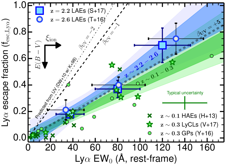
Figure 1: The relation between $\rm f_{esc,Ly\alpha}$ and Ly$\alpha$ EW₀ for $z\sim 2.2$ (stacks; see Sobral et al. 2017), $z\sim 2.6$ (binning; Trainor et al. 2015) and comparison with $z\sim 0-0.3$ samples (e.g. Cardamone et al. 2009; Hayes et al. 2013; Henry et al. 2015; Yang et al. 2016, 2017; Verhamme et al. 2017), estimated from dust-corrected H$\alpha$ luminosities (Equation 1). We show the 1 $\sigma$ and 2 $\sigma$ range for the fits at $z\sim 2.2-2.6$ and $z\sim 0-0.3$ separately, and find them to be consistent within those uncertainties, albeit with a potential steeper relation at higher redshift. We find a combined best fitting relation given by $\rm f_{esc,Ly\alpha}=0.0048\,EW_{0}\pm 0.05$. The observed relation is significantly away from what would be predicted based on observed UV slopes between $\beta\approx-2$ and $\beta\approx-1$ for LAEs (see DW10, ) and would require $\beta\approx+5$ for a good fit using Equation 5. Such red $\beta$ slopes are not observed for LAEs. Modifying Equation 5 to include the effect of $\rm\xi_{\rm ion}$ and dust reveals that those physical parameters likely play an important role; see Sections 3.2 and 3.3.

2.4 Measuring the Ly$\alpha$ escape fraction ($f_{esc,Ly\alpha}$) with H$\alpha$

We use dust corrected H$\alpha$ luminosity to predict the intrinsic Ly$\alpha$ luminosity. We then compare the latter to the observed Ly$\alpha$ luminosity to obtain the Ly$\alpha$ escape fraction ($\rm f_{esc,Ly\alpha}$). Assuming case B recombination, a temperature of 10⁴ K and an electron density of 350 cm^-3, we can use the observed Ly$\alpha$ luminosity ($\rm L_{Ly\alpha}$), the observed H$\alpha$ luminosity ($\rm L_{H\alpha}$) and the dust extinction affecting $\rm L_{H\alpha}$ ($\rm A_{\rm H\alpha}$, in mag) to compute $\rm f_{esc,Ly\alpha}$ as:

$$f_{\rm esc,Ly\alpha}=\frac{\rm L_{\rm Ly\alpha}}{\rm 8.7\,L_{\rm H\alpha}\times 10^{0.4\times A_{\rm H\alpha}}}.$$ (1)

This means that with our assumptions so far, and provided that we know $\rm f_{esc,Ly\alpha}$, we can use the observed $\rm L_{Ly\alpha}$ to obtain the intrinsic H$\alpha$ luminosity. All sources or samples in this study have been corrected for dust extinction using Balmer decrements, either measured directly for individual sources, or by applying the median extinction for stacks or bins of sources. Therefore, one can use Ly$\alpha$ as a star formation rate (SFR) indicator following Kennicutt (1998) for a Salpeter (Chabrier) IMF $(0.1-100\,{\rm M}_{\sun})$:

$$\rm{\rm SFR_{Ly\alpha}\,[M_{\odot}\,yr^{-1}]}=\frac{7.9(4.4)\times 10^{-42}}{(1-f_{esc,LyC})}\,\,\frac{L_{\rm Ly\alpha}}{8.7\,f_{\rm esc,Ly\alpha}}$$ (2)

where $\rm f_{esc,LyC}$ is the escape fraction of ionising LyC photons (see e.g. Sobral et al. 2018a). In practice, $\rm f_{esc,LyC}$ is typically assumed to be $\approx 0$, but it may be $\approx 0.1-0.15$ for LAEs (see discussions in e.g. Matthee et al. 2017a; Verhamme et al. 2017).

2.5 Statistical fits and errors

For all fits and relations in this work (e.g. $\rm f_{esc,Ly\alpha}$ vs. EW₀), we vary each data-point or binned data-point within its full Gaussian probability distribution function independently (both in EW₀ and $\rm f_{esc,Ly\alpha}$), and re-fit 10,000 times. We present the best-fit relation as the median of all fits, and the uncertainties (lower and upper) are the 16 and 84 percentiles. For bootstrapped quantities (e.g. for fitting the low redshift sample) we obtain 10,000 samples randomly picking half of the total number of sources and computing that specific quantity. We fit relations in the form $y=Ax+B$.

3 Results and Discussion

3.1 The observed $\rm f_{esc,Ly\alpha}$-EW₀ relation at $z\sim 0.1-2.6$

Figure 1 shows that $\rm f_{esc,Ly\alpha}$ correlates with Ly$\alpha$ EW₀ with apparently no redshift evolution between $z=0-2.6$ (see also Verhamme et al. 2017; Sobral et al. 2017). We find that $\rm f_{esc,Ly\alpha}$ varies continuously from $\approx 0.2$ to $\approx 0.7$ for LAEs from the lowest ($\approx 30$ Å) to the highest ($\approx 120-160$ Å) Ly$\alpha$ rest-frame EWs. We use our samples at $z\sim 0-0.3$ and $z\sim 2.2-2.6$, separately and together, to obtain linear fits to the relation between $\rm f_{esc,Ly\alpha}$ and Ly$\alpha$ EW₀ (see §2.5). These fits allow us to provide a more quantitative view on the empirical relation and evaluate any subtle redshift evolution; see Table 1.

The relation between $\rm f_{esc,Ly\alpha}$ and Ly$\alpha$ EW₀ is statistically significant at 5 to 10 $\sigma$ for all redshifts. We note that all linear fits are consistent with a zero escape fraction for a null EW₀ (Table 1), suggesting that the trend is well extrapolated for weak LAEs with EW${}_{0}\approx 0-20$ Å. Furthermore, as Table 1 shows, the fits to the individual (perturbed) samples at different redshifts result in relatively similar slopes and normalisations within the uncertainties, and thus are consistent with the same relation from $z\sim 0$ to $z\sim 2.6$. Nevertheless, we note that there is minor evidence for a shallower relation at lower redshift for the highest EW₀ (Figure 1), but this could be driven by current samples selecting sources with more extreme properties (including LyC leakers). Given our findings, we decide to combine the samples and obtain joint fits, with the results shown in Table 1. The slope of the relation is consistent with being $\approx 0.005$ with a null $\rm f_{esc,Ly\alpha}$ for EW${}_{0}=0$ Å.

Table 1: The results from fitting the relation between $\rm f_{esc,Ly\alpha}$ and Ly$\alpha$ EW₀ as $\rm f_{esc,Ly\alpha}=A\times{\rm EW_{0}}+B$, with EW₀ in Å (see §2.5). [i: individual sources used for fitting; b: binned/averaged quantity used for fitting; B: bootstrap analysis when fitting each of the 10,000 times; G: each data bin is perturbed along its Gaussian probability distribution.]

Sample	A (Å-1)	B	[notes]
$z\sim 0-0.3$	$0.0041^{+0.0006}_{-0.0004}$	$0.00^{+0.03}_{-0.02}$	[i,B]
$z\sim 2.2$	$0.0056^{+0.0012}_{-0.0011}$	$0.00^{+0.05}_{-0.05}$	[b,G]
$z\sim 2.6$	$0.0054^{+0.0016}_{-0.0015}$	$0.01^{+0.11}_{-0.11}$	[b,G]
$z\sim 0-2.2$	$0.0045^{+0.0008}_{-0.0007}$	$0.00^{+0.06}_{-0.06}$	[b,G]
$z\sim 2.2-2.6$	$0.0056^{+0.0012}_{-0.0012}$	$0.00^{+0.07}_{-0.08}$	[b,G]
$z\sim 0-2.6$	$0.0048^{+0.0007}_{-0.0007}$	$0.00^{+0.05}_{-0.05}$	[b,G]

3.2 The $\rm f_{esc,Ly\alpha}$-EW₀ relation: expectation vs. reality

The existence of a relation between $\rm f_{esc,Ly\alpha}$ and EW₀ (Figure 1) is not surprising. This is because Ly$\alpha$ EW₀ is sensitive to the ratio between Ly$\alpha$ and the UV luminosities, which can be used as a proxy of $\rm f_{esc,Ly\alpha}$ (see e.g. Dijkstra & Westra 2010; Sobral et al. 2018a). However, the slope, normalisation and scatter of such relation depend on complex physical conditions such as dust obscuration, differential dust geometry, scattering of Ly$\alpha$ photons and the production efficiency of ionising photons compared to the UV luminosity, $\rm\xi_{\rm ion}$ (see e.g. Hayes et al. 2014; Dijkstra 2017; Matthee et al. 2017a; Shivaei et al. 2018).

While a relation between $\rm f_{esc,Ly\alpha}$ and EW₀ is expected, we can investigate if it simply follows what would be predicted given that both the UV and Ly$\alpha$ trace SFRs. In order to predict $\rm f_{esc,Ly\alpha}$ based on Ly$\alpha$ EW₀ we first follow DW10 who used the Kennicutt (1998) SFR calibrations for a Salpeter IMF and UV continuum measured (observed) at 1400 Å to derive:

$$\rm\frac{SFR_{Ly\alpha}}{SFR_{UV}}=f_{esc,Ly\alpha(DW10)}=\Big{(}\frac{C}{E}\Big{)}EW_{0},$$ (3)

where $C=\Big{(}\frac{\nu_{\rm Ly\alpha}}{\nu_{\rm UV}}\Big{)}^{-2-\beta}\approx 1.152^{-\beta-2}$ and $\beta$ is the UV slope (where L${}_{\lambda}\propto\lambda^{\beta}$). The Kennicutt (1998) SFR calibrations yield:

$$\rm E=\frac{1.4\times 10^{-28}\lambda_{Ly\alpha}}{\frac{7.9}{8.7}\times 10^{-42}\nu_{Ly\alpha}}=76.0\,{\rm\AA},$$ (4)

which allows a final parameterisation of $\rm f_{esc,Ly\alpha}$ as a function of EW₀ and with just one free parameter, the UV $\beta$ slope:

$$\rm f_{esc,Ly\alpha(DW10)}=\frac{1.152^{-\beta-2}}{76}EW_{0}$$ (5)

The DW10 methodology implicitly assumes a “canonical”, constant $\rm\xi_{\rm ion}=1.3\times 10^{25}$ Hz erg^-1 (Kennicutt 1998), and a unit ratio between Ly$\alpha$ and UV SFRs (assuming 100 Myr constant SFR; see also Sobral et al. 2018a, and Equation 6). DW10 do not explicitly include the effect of dust in their framework which means assuming $0.0$ mag of extinction in the UV ($\rm A_{UV}=0.0$). Such framework will therefore typically overestimate the predicted $\rm f_{esc,Ly\alpha}$. Also, note that in DW10 $\beta$ is simply a parameter used to extrapolate the UV continuum from rest-frame 1400 Å to 1216 Å, and thus no physical conditions change with $\beta$ (but see e.g. Popping et al. 2017; Narayanan et al. 2018).

As in DW10, we use two different UV slopes: $\beta=-2.0$ and $\beta=-1.0$, which encompass the majority of LAEs and result in $C=1.0$ and $C=0.87$, respectively ($C\approx 1.152^{-\beta-2}$; see Equation 5). Based on the best empirical fits obtained in Section 3.1, we would expect $C/E=0.0048$, which would yield $\beta\approx+5.13$. Indeed, allowing $\beta$ to vary freely within the DW10 framework (Equation 5) allows to obtain relatively good fits to the data/observations ( $\rm\chi^{2}_{reduced}\approx 1.2$) but only for extremely red UV slopes of $\beta\approx+5$, which are completely excluded by other independent observations of LAEs. We therefore conclude that predicting $\rm f_{esc,Ly\alpha}$ based on the ratio of Ly$\alpha$ to UV SFRs using EW₀ and the DW10 framework with realistic UV $\beta$ slopes significantly overestimates $\rm f_{esc,Ly\alpha}$ (as indicated by the dot-dashed lines in Figure 1). Observations reveal higher Ly$\alpha$ EW₀ (by a factor of just over $\sim 3$ higher than the canonical value) than expected for a given $\rm f_{esc,Ly\alpha}$. The results reveal processes that can boost the ratio between Ly$\alpha$ and UV (boosting EW₀), particularly by boosting Ly$\alpha$, or processes that reduce $\rm f_{esc,Ly\alpha}$.

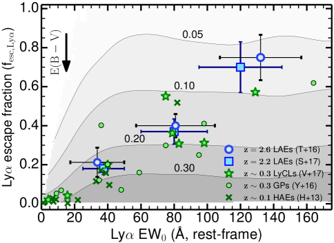
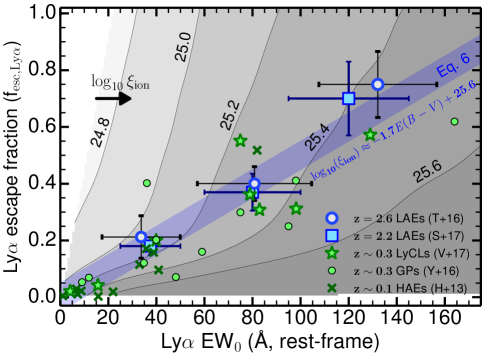
Figure 2: Left: The predicted $\rm f_{esc,Ly\alpha}$-Ly$\alpha$ EW₀ space for different $E(B-V)$ (contour levels) with our grid model (see §3.3 and Appendix A) and comparison with fits and implications by using Equation 6 (right). We find that increasing dust extinction drives $\rm f_{esc,Ly\alpha}$ down for a fixed EW₀, with data at $z\sim 0-2.6$ hinting for lower dust extinction at the highest EW₀ and higher dust extinction at the lowest EW₀, but with the range being relatively small overall and around $E(B-V)\approx 0.05-0.3$. Right: The predicted $\rm f_{esc,Ly\alpha}$-EW₀ space for different $\rm\xi_{ion}$ (contours). We find that while increasing $E(B-V)$ mostly shifts the relation down, increasing $\rm\xi_{ion}$ moves the relation primarily to the right.

Potential explanations include scattering, (differential) dust extinction, excitation due to shocks originating from stellar winds and/or AGN activity, and short time-scale variations in SFRs, leading to a higher $\xi_{\rm ion}$ (see Figure 1). High $\xi_{\rm ion}$ values ($\rm\xi_{\rm ion}\approx 3\times 10^{25}$ Hz erg^-1) seem to be typical for LAEs (e.g. Matthee et al. 2017a; Nakajima et al. 2018) and may explain the observed relation, but dust extinction likely also plays a role (see Figure 1 and Section 3.3). In order to further understand why the simple DW10 framework fails to reproduce the observations (unless one invokes $\beta\approx+5$), we expand on the previous derivations by identifying the role of $\rm\xi_{\rm ion}$ (see derivations in Sobral et al. 2018a) and dust extinction ($\rm A_{UV}$) in setting the relation between Ly$\alpha$ and UV SFRs and thus we re-write the relation between $\rm f_{esc,Ly\alpha}$ and EW₀ as:

$$\rm f_{esc,Ly\alpha}=\Big{(}\frac{1.152^{-\beta-2}}{76}EW_{0}\Big{)}\frac{1.3\times 10^{25}}{\xi_{ion}}10^{-0.4A_{UV}}$$ (6)

Note that Equation 6 (this study) becomes Equation 5 (DW10) if one assumes no dust extinction ($\rm A_{UV}=0$) and a canonical $\rm\xi_{\rm ion}=1.3\times 10^{25}$ Hz erg^-1. In order to keep the same framework as DW10 and avoid spurious correlations and conclusions, here we also let $\beta$ be decoupled from $\rm A_{UV}$ (but see Meurer et al. 1999, and Section 3.3). By allowing all 3 parameters to vary ($\beta=[-2.4,-1.5]$, $\rm\log_{10}[\xi_{ion}/Hz\,erg^{-1}]=[24.5,26.5]$ and $\rm A_{UV}=[0,1]$) independently in order to attempt to fit observations, we find best fit values of $\beta=-2.0\pm 0.3$, $\rm\log_{10}[\xi_{ion}/Hz\,erg^{-1}]=25.4\pm 0.1$ and $\rm A_{UV}=0.5\pm 0.3$ (corresponding to $E(B-V)=0.11\pm 0.07$ with a Calzetti et al. 2000 dust law). We find that $\rm\log_{10}\xi_{ion}$ is the only parameter that is relatively well constrained within our framework and that there is a clear degeneracy/relation between $\rm\log_{10}\xi_{ion}$ and dust extinction (higher dust extinction allows for a lower $\rm\log_{10}\xi_{ion}$, with a relation given by ${\rm\log_{10}[\xi_{ion}/Hz\,erg^{-1}]\approx-1.71}E(B-V)+25.6$ with $\beta=-2.0\pm 0.3$; see Figures 2 and 5) such that with no dust extinction one requires a high $\rm\log_{10}[\xi_{ion}/Hz\,erg^{-1}]=25.60\pm 0.05$ while for $\rm A_{UV}\approx 1.0$ a $\rm\log_{10}[\xi_{ion}/Hz\,erg^{-1}]\approx 25.25$ is required to fit the observations (Figure 5). Observations of LAEs point towards $\rm\log_{10}[\xi_{ion}/Hz\,erg^{-1}]\approx 25.5$ (e.g. Matthee et al. 2017a; Nakajima et al. 2018), in good agreement with our findings. If we fix $\rm\log_{10}[\xi_{ion}/Hz\,erg^{-1}]=25.5$, we still obtain a similar solution for $\beta$ (unconstrained), but we recover a lower $\rm A_{UV}=0.27\pm 0.15$ (corresponding to $E(B-V)=0.06\pm 0.04$ with a Calzetti et al. 2000 dust law), as we further break the degeneracy between $\rm A_{UV}$ and $\rm\xi_{ion}$. We find that canonical $\rm\log_{10}[\xi_{ion}/Hz\,erg^{-1}]=25.1$ values are strongly rejected and would only be able to explain the observations for significant amounts of dust extinction of $\rm A_{UV}\approx 1.5-2.0$ mag which are not found in typical LAEs.

In conclusion, we find that our modified analytical model (Equation 6, which expands the framework of DW10), is able to fit the observations relatively well. We find that high $\rm\xi_{ion}$ values of $\rm\log_{10}[\xi_{ion}/Hz\,erg^{-1}]=25.4\pm 0.1$ and some low dust extinction ($E(B-V)\approx 0.11$) are required to explain the observed relation between $\rm f_{esc,Ly\alpha}$ and EW₀. Without dust extinction one requires even higher ionisation efficiencies of $\rm\log_{10}[\xi_{ion}/Hz\,erg^{-1}]=25.60\pm 0.05$. In general, the physical values required to explain observations agree very well with observations and further reveal that LAEs are a population with high $\rm\log_{10}[\xi_{ion}/Hz\,erg^{-1}]\approx 25.4-25.6$ and low $E(B-V)\approx 0.1$.

3.3 The $\rm f_{esc,Ly\alpha}$-EW₀ relation: further physical interpretation

In order to further interpret the physics behind our observed empirical relation, we use a simple analytical toy model. In particular, we focus on the role of dust ($E(B-V)$) and $\xi_{\rm ion}$ (see details in Appendix A). We independently vary SFRs, $E(B-V)$ and $\xi_{\rm ion}$ with flat priors to populate the $\rm f_{esc,Ly\alpha}$-EW₀ space. The toy model follows our framework using a Calzetti et al. (2000) dust attenuation law and the Kennicutt (1998) calibrations and relations between UV and H$\alpha$. We also assume the same nebular and stellar continuum attenuation (see e.g. Reddy et al. 2015) and use the Meurer et al. (1999) relation. We also vary some assumptions independently which depend on the binary fraction, stellar metallicity and the IMF, which include the intrinsic Ly$\alpha$/H$\alpha$ ratio, the intrinsic UV $\beta$ slope (see e.g. Wilkins et al. 2013) and $\rm f_{esc,LyC}$ (see e.g. Table 2). Furthermore, we introduce an extra parameter to further vary $\rm f_{esc,Ly\alpha}$ and mimic processes which are hard to model, such as scattering, which can significantly reduce or even boost $\rm f_{esc,Ly\alpha}$ (Neufeld 1991) and allows our toy analytical model to sample a wide range of the $\rm f_{esc,Ly\alpha}$-EW₀ plane. We compute observed Ly$\alpha$ EW₀ and compare them with $\rm f_{esc,Ly\alpha}$ for 1,000,000 galaxy realisations. Further details are given in Appendix A.

The key results from our toy model are shown in Figure 2, smoothed with a Gaussian kernel of [0.07,20 Å] in the $\rm f_{esc,Ly\alpha}$-EW₀ parameter space. We find that both $E(B-V)$ and $\xi_{\rm ion}$ likely play a role in setting the $\rm f_{esc,Ly\alpha}$-EW₀ relation and changing it from simple predictions to the observed relation (see §3.2), a result which is in very good agreement with our findings in the previous section. As the left panel of Figure 2 shows, observed LAEs on the $\rm f_{esc,Ly\alpha}$-EW₀ relation seem to have low $E(B-V)\approx 0.1-0.2$, with the lowest EW₀ sources displaying typically higher $E(B-V)$ of 0.2-0.3 and the highest EW₀ sources likely having lower $E(B-V)$ of $<0.1$. Furthermore, as the right panel of Figure 2 shows, high EW₀ LAEs have higher $\xi_{\rm ion}$, potentially varying from $\rm\log_{10}(\xi_{\rm ion}/Hz\,erg^{-1})\approx 25$ to $\rm\log_{10}(\xi_{\rm ion}/Hz\,erg^{-1})\approx 25.4$. Our toy model interpretation is consistent with recent results (e.g. Trainor et al. 2016; Matthee et al. 2017a; Nakajima et al. 2018) for high EW₀ LAEs and with our conclusions in Section 3.2. Overall, a simple way to explain the $\rm f_{esc,Ly\alpha}$-EW₀ relation at $z\sim 0-2.6$ is for LAEs to have narrow ranges of low $E(B-V)\approx 0.1-0.2$, that may decrease slightly as a function of EW₀ and a relatively narrow range of high $\xi_{\rm ion}$ values that may increase with EW₀. Direct observations of Balmer decrements and of high excitation UV lines are required to confirm or refute our results.

Our toy model explores the full range of physical conditions independently without making any assumptions on how parameters may correlate, in order to interpret the observations in a simple unbiased way. However, the fact that observed LAEs follow a relatively tight relation between $\rm f_{esc,Ly\alpha}$ and EW₀ suggests that there are important correlations between e.g. dust, age and $\xi_{\rm ion}$. By selecting simulated sources in our toy model grid that lie on the observed relation (see Appendix A.1), we recover a tight correlation between $\xi_{\rm ion}$ and $E(B-V)$, while the full generated population in our toy model shows no correlation at all by definition (see Figure 5). This implies that the observed $\rm f_{esc,Ly\alpha}$-EW₀ relation could be a consequence of an evolutionary $\xi_{\rm ion}$-$E(B-V)$ sequence for LAEs, likely linked with the evolution of their stellar populations. For further details, see Appendix A.1. We note that the best fits to observations using Equation 6 are consistent with this possible relation as the solutions follow a well defined anti-correlation between $\xi_{\rm ion}$ and dust extinction with a similar relation and slope; see Figure 5 for a direct comparison.

3.4 Estimating $f_{esc,Ly\alpha}$ with a simple observable: Ly$\alpha$ EW₀

We find that LAEs follow a simple relation between $\rm f_{esc,Ly\alpha}$ and Ly$\alpha$ EW₀ roughly independently of redshift (for $z\leq 2.6$). Motivated by this, we propose the following empirical estimator (see Table 1) for $\rm f_{esc,Ly\alpha}$ as a function of Ly$\alpha$ EW₀ (Å):

$$\rm f_{esc,Ly\alpha}=0.0048^{+0.0007}_{-0.0007}\,{\rm EW_{0}}\pm 0.05\ \ [\,{\rm 0\leq EW_{0}\leq 160\,{\AA}}].$$ (7)

This relation may hold up to EW${}_{0}\approx 210$ Å, above which we would predict $\rm f_{esc,Ly\alpha}\approx 1$. This relation suggests that it is possible to estimate $\rm f_{esc,Ly\alpha}$ for LAEs within a scatter of 0.2 dex even if only the Ly$\alpha$ EW₀ is known/constrained. It also implies that the observed Ly$\alpha$ luminosities are essentially equal to intrinsic Ly$\alpha$ luminosities for sources with EW₀ as high as $\approx$ 200 Å. We conclude that while the escape of Ly$\alpha$ photons can depend on a range of properties in a very complex way (see e.g. Hayes et al. 2010; Matthee et al. 2016; Yang et al. 2017), using EW₀ and Equation 7 leads to predicting $\rm f_{esc,Ly\alpha}$ within $\approx 0.1-0.2$ dex of real values. This compares with a larger scatter of $\approx 0.3$ dex for relations with derivative or more difficult quantities to measure such as dust extinction or the red peak velocity of the Ly$\alpha$ line (e.g. Yang et al. 2017). We propose a linear relation for its simplicity and because current data do not suggest a more complex relation. Larger data-sets with H$\alpha$ and Ly$\alpha$ measurements, particularly those covering a wider parameter space (e.g. different sample selections, multiple redshifts and both high and low EWs), may lead to the necessity of a more complicated functional form. A departure from a linear fit may also provide further insight of different physical processes driving the relation and the scatter (e.g. winds, orientation angle, burstiness or additional ionisation processes such as fluorescence).

Equation 7 may thus be applied to estimate $\rm f_{esc,Ly\alpha}$ for a range of LAEs in the low and higher redshift Universe. For example, the green pea J1154+2443 (Izotov et al. 2018), has a measured $\rm f_{esc,Ly\alpha}$ directly from dust corrected H$\alpha$ luminosity of $\approx 0.7-0.8$, while Equation 7 would imply $\approx 0.6-0.7$ based on the $EW_{0}\approx 133$ Å for Ly$\alpha$, thus implying a difference of only 0.06-0.1 dex. Furthermore, in principle, Equation 7 could also be explored to transform EW₀ distributions (e.g. Hashimoto et al. 2017, and references therein) into distributions of $\rm f_{esc,Ly\alpha}$ for LAEs.

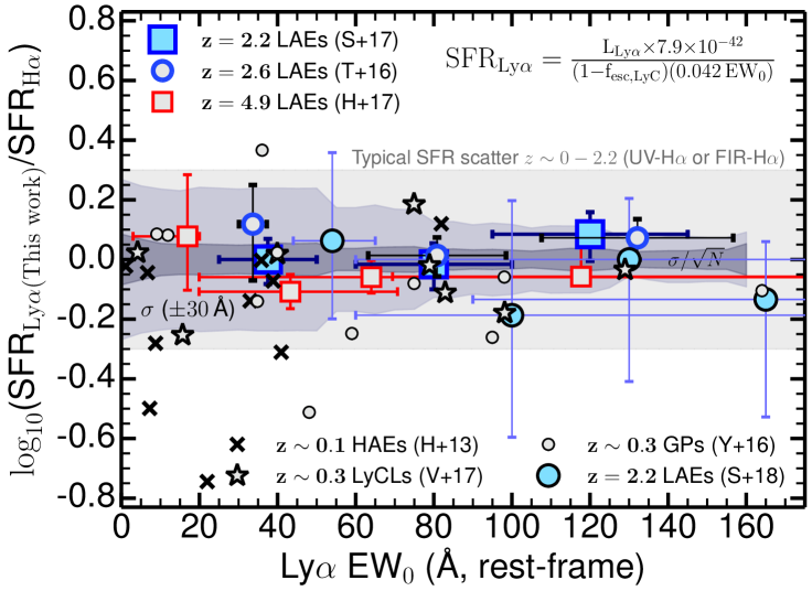
Figure 3: The logarithmic ratio between SFRs computed with Equation 8 using Ly$\alpha$ luminosity and EW₀ and the “true” SFR, measured directly from dust-corrected H$\alpha$ luminosity (given our definitions, $\log_{10}$(SFR${}_{\rm Ly\alpha(This\,\,work)}$/SFR${}_{\rm H\alpha})=\rm\log_{10}(f_{\rm esc,Ly\alpha(H\alpha)}/f_{\rm esc,Ly\alpha(This\,\,work)})$). The standard deviation ($\sigma$) and $\sigma$/$\sqrt{N}$ (N: number of sources) are computed in $\pm 30$ Å bins and indicated in light and darker grey. We find a relatively small scatter which may decrease for higher EWs and that is at the global level of $\pm 0.12$ dex for the typical definition of LAE at higher redshift (EW${}_{0}>20$ Å), but rises to $\approx 0.2$ dex at the lowest EWs. We also provide a comparison of the typical scatter between UV and FIR SFRs in relation to H$\alpha$ at $z\sim 0-2$ ($\approx 0.3$ dex; see e.g. Domínguez Sánchez et al. 2012; Oteo et al. 2015).

3.5 Ly$\alpha$ as an SFR indicator: empirical calibration and errors

Driven by the simple relation (Equation 7) found up to $z\sim 2.6$, we derive an empirical calibration to obtain SFRs based on two simple, direct observables for LAEs at high redshift: 1) Ly$\alpha$ EW₀ and 2) observed Ly$\alpha$ luminosity. This calibration is based on observables, but predicts the dust-corrected SFR. Based on Equations 2 and 7, for a Salpeter (Chabrier) IMF we can derive:

$${\rm SFR_{Ly\alpha}\,[{\rm M_{\odot}\,yr^{-1}}]}=\frac{{\rm L}_{\rm Ly\alpha}\times 7.9\,(4.4)\times 10^{-42}}{\rm(1-f_{esc,LyC})(0.042\,{\rm EW}_{0})}\,(\pm 15\%)$$ (8)

The current best estimate of the scatter in Equation 7 (the uncertainty in the relation to calculate $\rm f_{esc,Ly\alpha}$ is $\pm 0.05$) implies a $\pm 0.07$ dex uncertainty in the extinction corrected SFRs from Ly$\alpha$ with our empirical calculation. In order to investigate other systematic errors, we conduct a Monte Carlo analysis by randomly varying $\rm f_{esc,LyC}$ (0.0 to 0.2) and the case B coefficient (from 8.0 to 9.0), along with perturbing $\rm f_{esc,Ly\alpha}$ from $-0.05$ to $+0.05$. We assume that all properties are independent, and thus this can be seen as a conservative approach to estimate the uncertainties. We find that the uncertainty in $\rm f_{esc,Ly\alpha}$ is the dominant source of uncertainty (12%) with the uncertainty on $\rm f_{esc,LyC}$ and the case B coefficient contributing an additional 3% for a total of 15%. This leads to an expected uncertainty of Equation 8 of 0.08 dex.

Note that the SFR calibration presented in equation 8 follows Kennicutt (1998) and thus a solar metallicity, which may not be be fully applicable to LAEs, typically found to be sub-solar (Nakajima & Ouchi 2014; Steidel et al. 2016; Suzuki et al. 2017; Sobral et al. 2018b). Other caveats include the applicability of the Calzetti et al. (2000) dust law (see e.g. Reddy et al. 2016) and the shape and slope of the IMF used, although any other SFR calibration/estimator will share similar caveats.

3.6 Ly$\alpha$ as an SFR indicator: performance and implications

In Figure 3 we apply Equation 8 to compare the estimated SFRs (from Ly$\alpha$) with those computed with dust corrected H$\alpha$ luminosities. We also include individual sources at $z\sim 2.2$ (S18; Sobral et al. 2018b) and recent results from Harikane et al. (2018) at $z=4.8$ which were not used in the calibration, and thus provide an independent way to test our new calibration. We find a global scatter of $\approx 0.12$ dex, being apparently larger for lower EW₀, but still lower than the typical scatter between SFR indicators after dust corrections (e.g. UV-H$\alpha$ or FIR-H$\alpha$; see Domínguez Sánchez et al. 2012; Oteo et al. 2015), as shown in Figure 3. The small scatter and approximately null offset between our calibration’s prediction and measurements presented by Harikane et al. (2018) at $z\sim 5$ suggest that Equation 8 may be applicable at higher redshift with similarly competitive uncertainties (see §3.7 and §3.8). Nonetheless, we note that the measurements presented by Harikane et al. (2018) are inferred from broad-band IRAC photometry/colours as it is currently not possible to directly measure H$\alpha$ line luminosities beyond $z\sim 2.5$, and thus any similar measurements should be interpreted with some caution.

3.7 Application to bright and faint LAEs at high redshift

Our new empirical calibration of Ly$\alpha$ as an SFR indicator allows to estimate SFRs of LAEs at high redshift. The global Ly$\alpha$ luminosity function at $z\sim 3-6$ has a typical Ly$\alpha$ luminosity (L${}^{\star}_{\rm Ly\alpha}$) of 10^42.9 erg s^-1 (see e.g. Drake et al. 2017b; Herenz et al. 2017; Sobral et al. 2018a, and references therein), with these LAEs having EW${}_{0}\approx 80$ Å (suggesting $\rm f_{esc,Ly\alpha}=0.38\pm 0.05$ with Equation 7), which implies SFRs of $\approx 20$ M_⊙ yr^-1. If we explore the public SC4K sample of LAEs at $z\sim 2-6$ (Sobral et al. 2018a), limiting it to sources with up to EW${}_{0}=210$ Å and that are consistent with being star-forming galaxies ($\rm L_{Ly\alpha}<10^{43.2}$ erg s^-1; see Sobral et al. 2018b), we find a median SFR for LAEs of $12^{+9}_{-5}$ M_⊙ yr^-1, ranging from $\approx 2$ M_⊙ yr^-1 to $\approx 90$ M_⊙ yr^-1 at $z\sim 2-6$. These reveal that “typical” to luminous LAEs are forming stars below and up to the typical SFR (SFR${}^{\star}\approx 40-100$ M_⊙ yr^-1) at high redshift (see Smit et al. 2012; Sobral et al. 2014); see also Kusakabe et al. (2018).

Deep MUSE Ly$\alpha$ surveys (e.g. Drake et al. 2017a; Hashimoto et al. 2017) are able to sample the faintest LAEs with a median L${}_{\rm Ly\alpha}=10^{41.9\pm 0.1}$ erg s^-1 and EW${}_{0}=87\pm 6$ (Hashimoto et al. 2017) at $z\sim 3.6$. We predict a typical $\rm f_{esc,Ly\alpha}=0.42\pm 0.05$ and SFR${}_{\rm Ly\alpha}=1.7\pm 0.3$ M_⊙ yr^-1 for those MUSE LAEs. Furthermore, the faintest LAEs found with MUSE have L${}_{\rm Ly\alpha}=10^{41}$ erg s^-1 (Hashimoto et al. 2017), implying SFRs of $\approx 0.1$ M_⊙ yr^-1 with our calibration. Follow-up JWST observations targeting the H$\alpha$ line for faint MUSE LAEs are thus expected to find typical H$\alpha$ luminosities of $2\times 10^{41}$ erg s^-1 and as low as $\approx 1-2\times 10^{40}$ erg s^-1 for the faintest LAEs. Based on our predicted SFRs, we expect MUSE LAEs to have UV luminosities from $\rm M_{UV}\approx-15.5$ for the faintest sources (see e.g. Maseda et al. 2018), to $\rm M_{UV}\approx-19$ for more typical LAEs, thus potentially linking faint LAEs discovered from the ground with the population of SFGs that dominate the faint end of the UV luminosity function (e.g. Fynbo et al. 2003; Gronke et al. 2015; Dressler et al. 2015).

3.8 Comparison with UV and implications at higher redshift

Equations 7 and 8 can be applied to a range of spectroscopically confirmed LAEs in the literature. We also extend our predictions to sources within the epoch of re-ionisation, although there are important caveats on how the Ly$\alpha$ transmission is affected by the IGM; see e.g. Laursen et al. (2011).

We explore a recent extensive compilation by Matthee et al. (2017c) of both Ly$\alpha$- and UV-selected LAEs with spectroscopic confirmation and Ly$\alpha$ measurements (e.g. Ouchi et al. 2008, 2009; Ono et al. 2012; Sobral et al. 2015; Zabl et al. 2015; Stark et al. 2015c; Ding et al. 2017; Shibuya et al. 2018); see Table 3. These include published L_Lyα, EW₀ and M_UV. In order to correct UV luminosities we use the UV $\beta$ slope, typically used to estimate $\rm A_{UV}$. We use $\beta$ values (and errors) estimated in the literature for each source when available. When individual $\beta$ values are not available, we use $\beta=-1.6\pm 0.2$ for UV-selected sources (typical for their UV luminosity; e.g. Bouwens et al. 2009), while for the luminous LAEs we use $\beta=-1.9\pm 0.2$. As a comparison, we also use a fixed $\beta=-1.6\pm 0.2$ for all the sources, which leads to a correction of $\rm A_{UV}\approx 1.25$ mag. We list UV $\beta$ slopes and resulting SFRs in Table 3.

We predict (dust-corrected) SFRs using L_Lyα and EW₀ only (Equation 8) and compare with SFRs measured from dust-corrected UV luminosities (Kennicutt 1998); see Table 3. We make the same assumptions and follow the same methodology to transform the observables of our toy model/grid into SFRs (see Figure 4). We note that, as our simulation shows, one expects a correlation even if our calibration of Ly$\alpha$ as an SFR indicator is invalid at high redshift, but our grid shows that the scatter depends significantly on dust extinction. Therefore, we focus our discussion on the normalisation of the relation and particularly on the scatter, not on the existence of a relation. We also note that our calibration is based on dust corrected H$\alpha$ luminosities at $z\sim 0-2.6$, and that UV luminosities are not used prior to this Section.

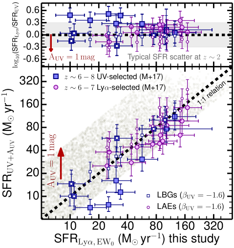
Figure 4: Comparison between SFRs computed with our new empirical calibration for Ly$\alpha$ as an SFR indicator (Equation 8) and those computed based on dust corrected UV luminosity (see §3.8) for a compilation of $z\sim 5-8$ sources (see Matthee et al. 2017c, and references therein). Our simple empirical calibration of Ly$\alpha$ as a SFR is able to recover dust corrected UV SFRs for the most star-forming sources, with a typical scatter of $\approx 0.2-0.3$ dex (the scatter is lower if one assumes a fixed $\beta=-1.6\pm 0.2$). For the sources with the lowest UV SFRs we find that Equation 8 seems to over-predict SFRs, potentially due to IGM effects which can lead to a lower EW₀. We also compute SFRs in the same way with observables from our toy model and show the results of all realisations in grey. We find that the scatter in our toy model is much larger, with this being driven by $E(B-V)$ being able to vary from 0.0 to 0.5.

Our results are shown in Figure 4 (see Table 3 for details on individual sources), which contains sources at a variety of redshifts, from $z\sim 6$ to $z\sim 8$ (e.g. Oesch et al. 2015; Stark et al. 2017). We find a good agreement between our predicted Ly$\alpha$ SFRs based solely on Ly$\alpha$ luminosities and EW₀ and the dust corrected UV SFRs for sources with the highest SFRs at $z\sim 6-8$ (Figure 4), with a scatter of $\approx 0.2-0.3$ dex. Interestingly, Equation 8 seems to over-predict (compared to the UV) Ly$\alpha$ SFRs for the least star-forming sources ($\leq 30-40$ M_⊙ yr^-1). This is caused by their typically very low EW₀, which would imply a low $\rm f_{esc,Ly\alpha}$, thus boosting the Ly$\alpha$ SFR compared to the UV. Taken as a single population, the UV-selected sources (LBGs) show a higher $\rm\log_{10}(SFR_{Ly\alpha}/SFR_{UV})=0.23\pm 0.24$ than LAEs that reveal $\rm\log_{10}(SFR_{Ly\alpha}/SFR_{UV})=0.15\pm 0.13$. Such discrepancies could be caused by the IGM which could be reducing the EW₀ and $\rm f_{esc,Ly\alpha}$. This would happen preferentially for the UV selected and for the sources with the lowest SFRs without strong Ly$\alpha$ in a way that our calibration at $z\sim 0-2.6$ simply does not capture. However, the deviation from a ratio of 1 is not statistically significant given the uncertainties and there is a large scatter from source to source to be able to further quantify the potential IGM effect.

Overall, our results and application to higher redshift reveals that Equation 8 is able to retrieve SFRs with very simple observables even for LAEs within re-ionisation (e.g. Ono et al. 2012; Stark et al. 2015c, 2017; Schmidt et al. 2017), provided they are luminous enough. In the early Universe the fraction of sources that are LAEs is higher (e.g. Stark et al. 2010, 2017; Caruana et al. 2018), thus making our calibration potentially applicable to a larger fraction of the galaxy population, perhaps with an even smaller scatter due to the expected narrower range of physical properties and more compact sizes (see discussions in e.g. Paulino-Afonso et al. 2018). Our calibration of Ly$\alpha$ as an SFR indicator is simple, directly calibrated with H$\alpha$, and should not have a significant dependence on metallicity, unlike other proposed SFRs tracers at high redshift such as [Cii] luminosity or other weak UV metal lines.

It is surprising that our calibration apparently still works even at $z\sim 7-8$ for the most luminous LAEs. This seems to indicate that the IGM may not play a significant role for these luminous Ly$\alpha$-visible sources, potentially due to early ionised bubbles (see e.g. Matthee et al. 2015, 2018; Mason et al. 2018a, b) or velocity offsets of Ly$\alpha$ with respect to systemic (see e.g. Stark et al. 2017). Interestingly, we find offsets between our calibration and the computed UV SFRs for the faintest sources, hinting that IGM effects start to be much more noticeable for such faint sources which may reside in a more neutral medium and/or on smaller ionised bubbles. Further observations measuring the velocity offsets between the Ly$\alpha$ and systemic redshifts for samples of LAEs within the epoch of re-ionisation and those at $z\sim 3-5$ will allow to check and test the validity of the relation within the epoch of re-ionisation.

3.9 A tool for re-ionisation: predicting the LyC luminosity

Based on our results and assumptions (see §2.4), we follow Matthee et al. (2017a) and derive a simple expression to predict the number of produced LyC photons per second, $\rm Q_{ion}$ (s^-1) with direct Ly$\alpha$ observables (L_Lyα and EW₀):

$$\rm Q_{ion,Ly\alpha}\,[{\rm s^{-1}}]=\frac{{\rm L}_{\rm Ly\alpha}}{\rm c_{H\alpha}\,(1-f_{esc,LyC})\,(0.042\,{\rm EW}_{0})},$$ (9)

where $\rm c_{H\alpha}=1.36\times 10^{-12}$ erg (e.g. Kennicutt 1998; Schaerer 2003), under our case B recombination assumption (see §2.4). We caution that Equation 9 may not be fully valid for all observed LAEs within the epoch of reionisation. This is due to possible systematic effects on EW₀ of an IGM which is partly neutral, although we note that as found in Section 3.8 it may well be valid for the most luminous LAEs at $z\sim 7-8$.

Recent work by e.g. Verhamme et al. (2017) show that LyC leakers are strong LAEs, and that $\rm f_{esc,Ly\alpha}$ is linked and/or can be used to predict $\rm f_{esc,LyC}$ (see Chisholm et al. 2018). Equation 9 provides an extra useful tool: an empirical simple estimator of $\rm Q_{ion}$ for LAEs given observed Ly$\alpha$ luminosities and EW₀. Note that Equation 9 does not require measuring UV luminosities or $\xi_{\rm ion}$, but instead direct, simple observables. Matthee et al. (2017c) already used a similar method to predict $\xi_{\rm ion}$ at high redshift. Coupled with an accurate estimate of the escape fraction of LyC photons from LAEs (see e.g. Steidel et al. 2018), a robust estimate of the full number density of LAEs from faint to the brightest sources (Sobral et al. 2018a) and their redshift evolution, Equation 9 may provide a simple tool to further understand if LAEs were able to re-ionise the Universe.

4 Conclusions

Ly$\alpha$ is intrinsically the brightest emission-line in active galaxies, and should be a good SFR indicator. However, the uncertain and difficult to measure $\rm f_{esc,Ly\alpha}$ has limited the interpretation and use of Ly$\alpha$ luminosities. In order to make progress, we have explored samples of LAEs at $z=0-2.6$ with direct Ly$\alpha$ escape fractions measured from dust corrected H$\alpha$ luminosities which do not require any SED fitting, $\rm\xi_{ion}$ or other complex assumptions based on derivative quantities. Our main results are:

$\bullet$  

There is a simple, linear relation between $\rm f_{esc,Ly\alpha}$ and Ly$\alpha$ EW₀: $\rm f_{esc,Ly\alpha}=0.0048\,EW_{0}[{\AA}]\pm 0.05$ (Equation 7) which is shallower than simple expectations, due to both more ionising photons per UV luminosity ($\rm\xi_{ion}$) and low dust extinction ($E(B-V)$) for LAEs (Figure 1). This allows the prediction of $\rm f_{esc,Ly\alpha}$ based on a simple direct observable, and thus to compute the intrinsic Ly$\alpha$ luminosity of LAEs at high redshift.

$\bullet$  

The observed $\rm f_{esc,Ly\alpha}$-EW₀ can be explained by high $\rm\xi_{ion}$ and low $E(B-V)$ or, more generally, by a tight $\rm\xi_{ion}$-$E(B-V)$ sequence for LAEs, with higher $\rm\xi_{ion}$ implying lower $E(B-V)$ and vice versa. $\rm\xi_{ion}$ and $E(B-V)$ may vary within the $\rm f_{esc,Ly\alpha}$-EW₀ plane (Figure 2). Our results imply that the higher the EW₀ selection, the higher the $\rm\xi_{ion}$ and the lower the $E(B-V)$.

$\bullet$  

The $\rm f_{esc,Ly\alpha}$-EW₀ relation reveals a scatter of only 0.1-0.2 dex for LAEs, and there is evidence for the relation to hold up to $z\sim 5$ (Figure 3). The scatter is higher towards lower EW₀, consistent with a larger range in galaxy properties for sources with the lowest EW₀. At the highest EW₀, on the contrary, the scatter may be as small as $\approx 0.1$ dex, consistent with high EW₀ LAEs being an even more homogeneous population of dust-poor, high ionisation star-forming galaxies.

$\bullet$  

We use our results to calibrate Ly$\alpha$ as an SFR indicator for LAEs (Equation 8) and find a global scatter of 0.2 dex between measurements using Ly$\alpha$ only and those using dust-corrected H$\alpha$ luminosities. Such scatter seems to depend on EW₀, being larger at the lowest EW₀. Our results also allow us to derive a simple estimator of the number of LyC photons produced per second (Equation 9) with applications to studies of the epoch of re-ionisation.

$\bullet$  

Equation 8 implies that star-forming LAEs at $z\sim 2-6$ have SFRs typically ranging from 0.1 to 20 M_⊙ yr^-1, with MUSE LAEs expected to have typical SFRs of $1.7\pm 0.3$ M_⊙ yr^-1, and more luminous LAEs having SFRs of $12^{+9}_{-5}$ M_⊙ yr^-1.

$\bullet$  

SFRs based on Equation 8 are in good agreement with dust corrected UV SFRs even within the epoch of re-ionisation for SFRs higher than $\approx 30-40$ M_⊙ yr^-1, hinting for it to be applicable in the very early Universe for bright enough LAEs. For lower SFRs we find that Equation 8 may over-predict SFRs compared to the UV, potentially due to IGM effects. If shown to be the case, our results have implications for the minor role of the IGM in significantly changing Ly$\alpha$ luminosities and EW₀ for the most luminous LAEs within the epoch of re-ionisation.

Our results provide a simple interpretation of the tight $\rm f_{esc,Ly\alpha}$-EW₀ relation. Most importantly, we provide simple and practical tools to estimate $\rm f_{esc,Ly\alpha}$ at high redshift with two direct observables and thus to use Ly$\alpha$ as an SFR indicator and to measure the number of ionising photons from LAEs. The empirical calibrations presented here can be easily tested with future observations with JWST which can obtain H$\alpha$ and H$\beta$ measurements for high-redshift LAEs.

Appendix A Toy-model grid for $\rm f_{esc,Ly\alpha}$ dependencies

We construct a simple analytical toy-model grid to produce observable H$\alpha$, UV and Ly$\alpha$ luminosities and EW₀ from a range of input physical conditions (see Table 2). We independently sample in steps of 0.01 or 0.01 dex combinations of SFR, $\rm f_{esc,LyC}$, case B Ly$\alpha$/H$\alpha$ intrinsic ratio, $\rm\log_{10}(\xi_{ion}/Hz\,erg^{-1})$, $E(B-V)$ with a Calzetti et al. (2000) dust attenuation law and a parameter to control $\rm f_{esc,Ly\alpha}$ (from e.g. scattering leading to higher dust absorption or scattering Ly$\alpha$ photons away from or into the observers’ line of sight) which acts as a further factor affecting $\rm f_{esc,Ly\alpha}$; see Table 2 for the range in parameters explored independently. We follow Kennicutt (1998) and all definitions and assumptions mentioned in this paper and we sample the parameter space with a flat prior. We use the Meurer et al. (1999) relation: $\rm A_{UV}\approx 4.43+1.99\beta$ (based on an intrinsic slope $\beta_{int}=-2.23$), but we also vary the intrinsic $\beta_{int}$ from $-2.6$ to $-1.8$ (see e.g. Wilkins et al. 2013). We publicly release our simple python script which can be used for similar studies and/or to study different ranges in the parameter space, or conduct studies in which properties are intrinsically related/linked as one expects for realistic galaxies. Section A.2 presents the full equations implemented in the publicly available python script.

Table 2: The parameters varied in our simple toy model to produce a grid of 1,000,000 sources to interpret the observational results (see Appendix A).

Property	Minimum	Maximum	$\Delta$ param.
SFR (M⊙ yr-1)	0.1	100	0.01 dex
$\rm\log_{10}(\xi_{ion}/Hz\,erg^{-1})$	24.7	26.5	0.01 dex
$\rm f_{esc,LyC}$	0.0	0.15	0.01
Ly$\alpha$/H$\alpha$	8.0	9.0	0.01
$E(B-V)$	0.0	0.5	0.01
$\rm\beta_{int}$	$-2.6$	$-1.8$	0.01
Extra $\rm f_{esc,Ly\alpha}$	0.0	1.3	0.01

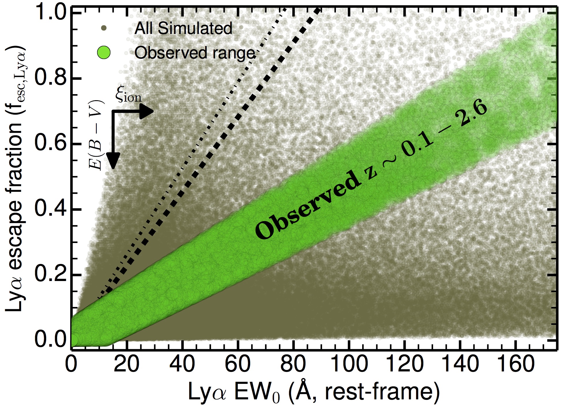
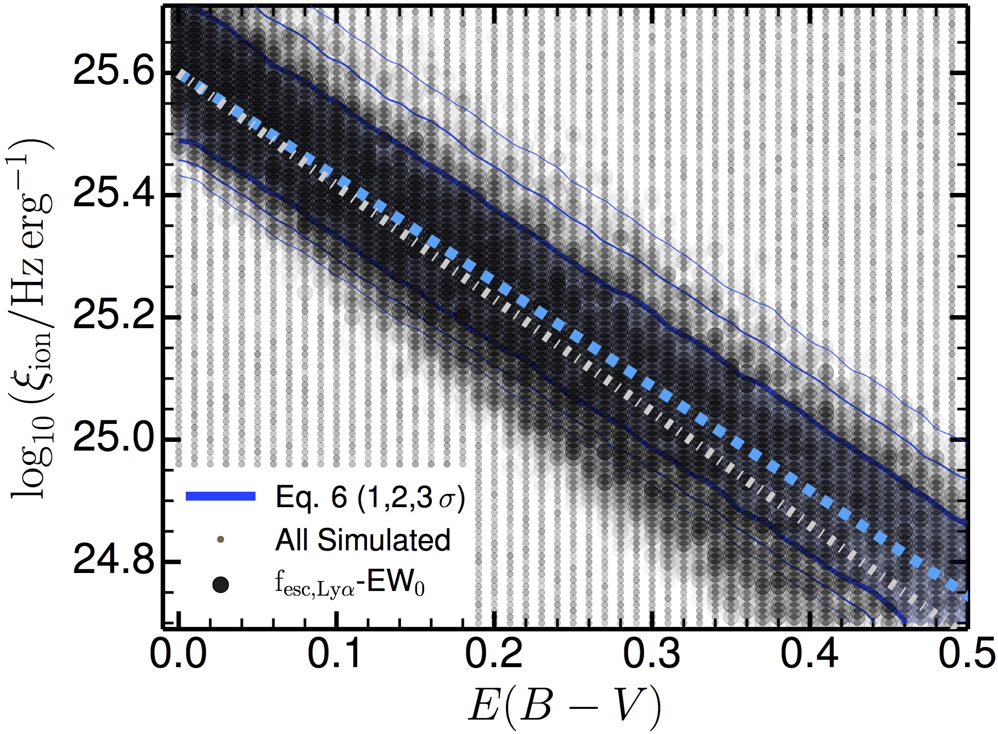
Figure 5: Left: The predicted relation between $\rm f_{esc,Ly\alpha}$ and Ly$\alpha$ EW₀ for our toy model, which shows little to no correlation by sampling all physical parameters independently (see Table 2). We also show the observed range ($\approx\pm 0.05$) which is well constrained at $z\sim 0-2.6$. We use simulated sources that are consistent with observations of LAEs to explore the potential reason behind the observed tight $\rm f_{esc,Ly\alpha}$-EW₀ correlation for LAEs. Right: By restricting our toy model to the observed relation and its scatter, we find a relatively tight $\rm\xi_{ion}$-$E(B-V)$ anti-correlation for LAEs (EW${}_{0}>25$ Å): $\rm\log_{10}(\xi_{ion}/Hz\,erg^{-1})\approx-1.85\times\,E(B-V)+25.6$ (shown as grey dot-dashed line). This is in good agreement with the family of best fits using Equation 6 (we show the 1, 2 and 3 $\sigma$ contours) which yields $\rm\log_{10}(\xi_{ion}/Hz\,erg^{-1})\approx-1.71\times\,E(B-V)+25.6$, with only a small difference in the slope. The highest observed EW₀ correspond to the highest $\rm\xi_{ion}$ and the lowest $E(B-V)$, while lower EW₀ leads to a lower $\rm\xi_{ion}$ and a higher $E(B-V)$. Our results thus show that the observed $\rm f_{esc,Ly\alpha}$-EW₀ correlation for LAEs at $z\sim 0-2.6$ only allows a well defined $\xi_{ion}$-$E(B-V)$ sequence that may be related with important physics such as the age of the stellar populations, their metallicity, dust production and how those evolve together.

A.1 The $\rm f_{esc,Ly\alpha}$-EW₀ and a potential $\xi_{ion}$-$E(B-V)$ sequence for LAEs

We use our simple analytical model to further interpret the observed relation between $\rm f_{esc,Ly\alpha}$-EW₀ and its tightness. We take all artificially generated sources and select those that satisfy the observed relation given in Equation 7, including its scatter (see Figure 5). We further restrict the sample to sources with Ly$\alpha$ EW${}_{0}>25$ Å. We find that along the observed $\rm f_{esc,Ly\alpha}$-EW₀ relation, LAEs become less affected by dust extinction as a function of increasing EW₀, while $\rm\xi_{ion}$ increases, as already shown in §3.3 and Figure 2.

In the right panel of Figure 5 we show the full parameter range explored in $\rm\xi_{ion}$-$E(B-V)$. By constraining the simulated sources with the observed $\rm f_{esc,Ly\alpha}$-EW₀ relation, we obtain a tight ($\pm 0.1$ dex), linear relation between $\rm\log_{10}\xi_{ion}$ and $E(B-V)$ given by $\rm\log_{10}(\xi_{ion}/Hz\,erg^{-1})\approx-1.85\times\,E(B-V)+25.6$. This means that in order for simulated sources to reproduce observations, LAEs should follow a very well defined $\rm\xi_{ion}$-$E(B-V)$ sequence with high $\rm\xi_{ion}$ values corresponding to very low $E(B-V)$ (mostly at high EW₀ and high $\rm f_{esc,Ly\alpha}$) and higher $E(B-V)$ to lower $\rm\xi_{ion}$ (mostly at low EW₀ and high $\rm f_{esc,Ly\alpha}$). Our results thus hint for the $\rm f_{esc,Ly\alpha}$-EW₀ to be driven by the physics (and diversity) of young and metal poor stellar populations and their evolution.

A.2 Steps and equations for the model grid

We produce a model grid with our simple toy model which implements all equations and follows the observationally-motivated methodology used in the paper for full self-consistency. For each of the $N=1,000,000$ realisations, the script randomly picks (with a flat prior) parameters out of the parameter grid presented in Table 2 (independently, per parameter).

The following steps are then taken per realisation. The H$\alpha$ luminosity is computed using the Kennicutt (1998) calibration and the Ly$\alpha$ luminosity is obtained by using the case B coefficient used for that specific realisation. The UV SFR is computed by using $\rm\log_{10}(\xi_{ion}/Hz\,erg^{-1})$ for that realisation and the Kennicutt (1998) calibration, which is then used to compute the intrinsic UV luminosity at rest-frame 1600 Å ($M_{UV}$ and L_UV). This step produces all the intrinsic luminosities which will be used: Ly$\alpha$, UV and H$\alpha$.

Next, by using the randomly picked value of $E(B-V)$ (see Table 2), the Calzetti et al. (2000) attenuation law is used. For simplicity, as mentioned before, we set the attenuation of the nebular lines to be the same as the stellar continuum. We use the Calzetti et al. (2000) dust attenuation law to compute $A_{\lambda}$ (mag) for $\lambda=1215.7,1600,6563$ Å in order to compute the attenuation at Ly$\alpha$, UV and H$\alpha$. We then compute the observed Ly$\alpha$, UV and H$\alpha$ luminosities after dust attenuation by computing:

$$\rm L_{\lambda,observed}=L_{\lambda,intrinsic}\times 10^{-0.4\,A_{\lambda}}$$ (10)

Finally, for Ly$\alpha$, we apply the parameter “Extra $\rm f_{esc,Ly\alpha}$” (see Table 2) which is multiplied by the observed Ly$\alpha$ luminosity (attenuated by dust) to produce the final observed Ly$\alpha$ luminosity. This is to quantify our ignorance on radiative transfer effects which are not explicitly modelled and are extremely complex. Following the methodology in this paper, the Ly$\alpha$ escape fraction is then computed using equation 1 and with all quantities computed or randomly picked with the script.

Finally, after randomly picking an intrinsic $\beta_{int}$ slope, the Meurer et al. (1999) relation is used to transform $E(B-V)$ into an observed $\beta$ UV slope. This follows Meurer et al. (1999) and assumes that LAEs have $\beta=\beta_{int}$ for $E(B-V)=0.0$. $\beta$ is then used together with the observed UV luminosity at 1600 Å to compute the observed UV luminosity at $\lambda=1215.7$ Å. This is used to compute the observed EW₀. The toy model also computes the intrinsic EW₀, i.e., the rest-frame Ly$\alpha$ EW in the case of no dust and no scattering. The script also applies the calibrations derived/obtained or used in the paper to predict the Ly$\alpha$ escape fraction, Ly$\alpha$ and UV SFRs based on equations 7 and 8 (see also Section 3.8) and the input from the simulation grid. These may be interesting for readers to explore further trends, and are provided as further information in the catalogue of 1,000,000 simulated sources.

Appendix B Data used for the high-redshift comparison between UV and Ly$\alpha$ SFRs

Table 3: Application to high redshift UV-continuum and Ly$\alpha$ selected LAEs (see compilation by Matthee et al. 2017c). Errors on Ly$\alpha$ luminosity and EW₀ are assumed to be $\approx 0.1$ dex, while errors on $\rm M_{UV}$ are taken as $\approx 0.2$ dex. We compute the UV SFRs (SFR_UV, dust corrected) using Kennicutt (1998) and $\beta$ values, individually measured when available, or $\beta=-1.6\pm 0.2$ for UV-selected and $\beta=-1.9\pm 0.2$ for Ly$\alpha$ selected sources when not available. Furthermore, we also compute dust corrected UV SFRs by using $\beta=-1.6\pm 0.2$ for all sources (SFR${}^{\beta=-1.6}_{\rm UV}$). Ly$\alpha$ SFRs (SFR_Lyα; calibrated to be dust-corrected) are computed with our Equation 8. Notes: 1: EW₀ have been recomputed and rest-framed when compared to original reference. 2: $\rm M_{UV}$ have been recomputed when compared to original reference. 3: Values used are from Zabl et al. (2015). 4: Computed as in Matthee et al. (2017b). 5: COLA1’s discovery is reported in Hu et al. (2016); here we use the latest measurements from Matthee et al. (2018). 6: $\beta$ values not available; calculated assuming $\beta=-1.6\pm 0.2$. 7: $\beta$ values not available; calculated assuming $\beta=-1.9\pm 0.2$. This table is also provided in fits format.

Name	$z$	$\rm log_{10}(L_{Ly\alpha})$	EW0	MUV	$\beta_{\rm UV}$	SFR${}^{\beta}_{\rm UV}$	SFR${}^{\beta=-1.6}_{\rm UV}$	SFRLyα	Reference
(UV selected)		[erg s-1]	[Å]	[mag]		[M⊙ yr-1]	[M⊙ yr-1]	[M⊙ yr-1]
A383-5.2	6.03	$42.8$	$138$	$-19.3$	$\beta^{6}$	$10^{+5}_{-3}$	$10^{+3}_{-3}$	$11^{+4}_{-3}$	Stark et al. (2015c)
RXCJ22-ID3	6.11	$42.5$	$40$	$-20.1$	$-2.3\pm 0.2$	$7^{+2}_{-1}$	$21^{+7}_{-5}$	$16^{+8}_{-5}$	Mainali et al. (2017)
RXCJ22-4431	6.11	$42.9$	$68$	$-20.2$	$-2.3\pm 0.2$	$8^{+2}_{-1}$	$23^{+8}_{-6}$	$25^{+11}_{-7}$	Schmidt et al. (2017)
SDF-46975	6.84	$43.2$	$43$	$-21.5$	$\beta^{6}$	$76^{+37}_{-25}$	$76^{+26}_{-20}$	$75^{+35}_{-22}$	Ono et al. (2012)
IOK-1	6.96	$43.0$	$42$	$-21.3$	$-2.0\pm 0.3$	$31^{+15}_{-9}$	$63^{+22}_{-16}$	$57^{+26}_{-17}$	Ono et al. (2012)
BDF-521	7.01	$43.0$	$64$	$-20.6$	$-2.3\pm 0.4$	$11^{+3}_{-2}$	$33^{+11}_{-9}$	$34^{+14}_{-10}$	Cai et al. (2015)
A1703 zd6	7.04	$42.5$	$65$	$-19.3$	$-2.4\pm 0.2$	$3^{+1}_{-1}$	$10^{+3}_{-3}$	$10^{+4}_{-3}$	Stark et al. (2015b)
BDF-3299	7.11	$42.8$	$50$	$-20.6$	$-2.0\pm 0.5$	$16^{+8}_{-5}$	$33^{+11}_{-9}$	$30^{+13}_{-9}$	Vanzella et al. (2011)
GLASS-stack	7.20	$43.0$	$210$	$-19.7$	$\beta^{6}$	$15^{+7}_{-5}$	$15^{+5}_{-4}$	$10^{+4}_{-3}$	Smidt et al. (2016)
EGS-zs8-2	7.48	$42.7$	$9$	$-21.9$	$-1.8\pm 0.4$	$77^{+37}_{-25}$	$110^{+37}_{-28}$	$102^{+205}_{-49}$	Stark et al. (2015a)
FIGSGN1-1292	7.51	$42.8$	$49$	$-21.2$	$\beta^{6}$	$58^{+29}_{-19}$	$58^{+20}_{-15}$	$31^{+14}_{-9}$	Tilvi et al. (2016)
GN-108036	7.21	$43.2$	$33$	$-21.8$	$\beta^{6}$	$100^{+52}_{-33}$	$100^{+35}_{-26}$	$99^{+49}_{-31}$	Stark et al. (2015a)
EGS-zs8-1	7.73	$43.1$	$21$	$-22.1$	$-1.7\pm 0.1$	$111^{+56}_{-37}$	$132^{+46}_{-34}$	$125^{+83}_{-43}$	Oesch et al. (2015)
(Ly$\alpha$ selected)
SR61	5.68	$43.4$	$210$	$-21.1$	$-1.8\pm 0.4$	$38^{+19}_{-13}$	$53^{+17}_{-14}$	$26^{+10}_{-7}$	Matthee et al. (2017c)
Ding-3	5.69	$42.8$	$62$	$-20.9$	$\beta^{7}$	$25^{+13}_{-8}$	$44^{+15}_{-11}$	$24^{+10}_{-7}$	Ding et al. (2017)
Ding-4	5.69	$42.3$	$106$	$-20.5$	$\beta^{7}$	$18^{+9}_{-6}$	$30^{+11}_{-7}$	$4^{+2}_{-1}$	Ding et al. (2017)
Ding-5	5.69	$43.2$	$79$	$-21.0$	$\beta^{7}$	$28^{+14}_{-9}$	$48^{+17}_{-12}$	$44^{+18}_{-12}$	Ouchi et al. (2008)
Ding-1	5.70	$43.0$	$21$	$-22.2$	$\beta^{7}$	$85^{+43}_{-28}$	$147^{+50}_{-38}$	$103^{+72}_{-35}$	Ding et al. (2017)
J2334542	5.73	$43.7$	$210$	$-21.5$	$\beta^{7}$	$44^{+22}_{-14}$	$76^{+27}_{-19}$	$50^{+20}_{-14}$	Shibuya et al. (2018)
J021835	5.76	$43.7$	$107$	$-21.7$	$\beta^{7}$	$53^{+26}_{-17}$	$92^{+31}_{-24}$	$94^{+39}_{-27}$	Shibuya et al. (2018)
VR71	6.53	$43.4$	$35$	$-22.5$	$-2.0\pm 0.3$	$97^{+48}_{-31}$	$192^{+65}_{-48}$	$149^{+72}_{-46}$	Matthee et al. (2017c)
J1621262	6.55	$43.9$	$99$	$-22.8$	$\beta^{7}$	$145^{+73}_{-48}$	$252^{+88}_{-64}$	$170^{+68}_{-48}$	Shibuya et al. (2018)
J160234	6.58	$43.5$	$81$	$-21.9$	$\beta^{7}$	$63^{+31}_{-21}$	$111^{+37}_{-28}$	$88^{+36}_{-25}$	Shibuya et al. (2018)
Himiko3	6.59	$43.6$	$65$	$-22.1$	$-2.0\pm 0.4$	$63^{+32}_{-19}$	$132^{+45}_{-33}$	$142^{+58}_{-42}$	Ouchi et al. (2009)
COLA1	6.59	$43.6$	$120$	$-21.6$	$\beta^{7}$	$48^{+24}_{-16}$	$83^{+29}_{-22}$	$73^{+29}_{-21}$	Matthee et al. (2018)
CR74	6.60	$43.9$	$211$	$-22.2$	$-2.3\pm 0.3$	$49^{+15}_{-9}$	$146^{+50}_{-37}$	$87^{+35}_{-25}$	Sobral et al. (2015)

Table 3 provides the data used for Figure 4, including individual measurements per source, their name and reference. Note that the data is taken from a compilation from Matthee et al. (2017c) with minor modifications for a few LAEs, as a indicated in Table 3.