Gaussian and exponential lateral connectivity on distributed spiking neural network simulation

Abstract

We measured the impact of long-range exponentially decaying intra-areal lateral connectivity on the scaling and memory occupation of a distributed spiking neural network simulator compared to that of short-range Gaussian decays. While previous studies adopted short-range connectivity, recent experimental neurosciences studies are pointing out the role of longer-range intra-areal connectivity with implications on neural simulation platforms. Two-dimensional grids of cortical columns composed by up to 11 M point-like spiking neurons with spike frequency adaption were connected by up to 30 G synapses using short- and long-range connectivity models. The MPI processes composing the distributed simulator were run on up to 1024 hardware cores, hosted on a 64 nodes server platform. The hardware platform was a cluster of IBM NX360 M5 16-core compute nodes, each one containing two Intel Xeon Haswell 8-core E5-2630 v3 processors, with a clock of 2.40 G Hz, interconnected through an InfiniBand network, equipped with 4$\times$ QDR switches.

I Introduction

We present the impact of the range of intra-areal lateral connectivity on the scaling of distributed point-like spiking neural network simulations when run on up to 1024 software processes (and hardware cores) for cortical models including tens of billions of synapses. A simulation including a few tens of billions of synapses is what is required to simulate the activity of one $cm^{2}$ of cortex at biological resolution (e.g. 54K neuron/$mm^{2}$ and about 5K synapses per neuron in the rat neocortex area [1]). The capability to scale a problem up to such a size allows simulating an entire cortical area. Our study focuses on the computational cost of the implementation of connectivities, pointed out in recent studies reporting about long range intra-areal lateral connectivity in many different cerebral areas, from cat primary visual cortex [2], to rat neocortex [1, 3], just as examples. For instance, in rat neocortex, the impact of lateral connectivity on the pyramidal cells in layer 2/3 and layer 6a, results in $\sim$75% of incoming remote synapses to neurons of these layers.

Longer-range intra-areal connectivity can be modeled by a distance-dependent exponential decay of the probability of synaptic connection between pairs of neurons: i.e. $A\cdot exp(\frac{-r}{\lambda}$), where r stands for the distance between neurons, $\lambda$ is the exponential decay constant and A is a normalization factor that fixes the total number of lateral connections. Decay constants in the range of several hundred microns are required to match experimental results.

Previous studies considered intra-areal synaptic connections dominated by local connectivity: e.g. [4] estimated at least 55% the fraction of local synapses, reaching also a ratio of 75%. Such shorter-range lateral connectivity has often been modeled with a distance dependent Gaussian decay [5] $B\cdot exp(\frac{-r^{2}}{2\sigma^{2}}$), where r stands again for distance between neurons, $\sigma^{2}$ is the variance that determines the lateral range and B fixes the total number of projections. Here we present measures about the scaling of simulations of cortical area patches of different sizes represented by two-dimensional grids of “cortical modules”. Each cortical module is composed of 1240 single-compartment, point-like neurons (no dendritic tree is represented) each one receiving up to $\sim$2390 recurrent synapses (instantaneous membrane potential charging) plus those bringing external stimuli. The larger simulated cerebral cortex tile includes 11.4 M neurons and 29.6 G total synapses. Exponentially decaying lateral connectivity (longer-range) are compared to a Gaussian connectivity decay (shorter-range), analyzing the scaling and the memory usage of our Distributed and Plastic Spiking Neural Network simulation engine (DPSNN in the following).

On DPSNN, the selection of the connectomic model has consequences due to: 1) the mapping strategy (neurons and incoming synapses are placed on MPI processes according to spatial contiguity) and, 2) synaptic messages exchanged between neurons simulated on different MPI processes entail communication tasks among those processes; the higher the number of lateral synaptic connections and the longer the interaction distance is, the more intensive the communication task among processes becomes.

The impact of other biologically plausible, or experimentally demonstrated, connectivity patterns is worth of investigation, but is not covered by this work. One of the directions could be the study of the effect of connectivity patterns with local modular/clustered connection and global (inter-areal) non-homogenoeus lateral connectivity. Such a connectivity has been studied theoretically for network dynamical behaviors on a small local neural network [6]. Experimentally, complex connectivity has been seen mostly for across-area studies, however see also the emerging strong evidence of local motifs [7].

The article is structured as follows: Section II describes the main features of the simulation engine and its distributed implementation; network models are summarized in Section III, with a specific description of the different schemes adopted for the lateral intra-area connectivity; Section IV reports the impact of lateral connectivity on the scaling. A discussion section closes the paper.

II Description of the Spiking Neural Network simulator

The main focus of several neural network simulation projects is the search for a) biological correctness; b) flexibility in biological modeling; c) scalability using commodity technology — e.g. NEST [8, 9], NEURON [10], GENESIS [11]. A second research line focuses more explicitly on computational challenges when running on commodity systems, with varying degrees of association to specific platform ecosystems [12, 13, 14, 15]. Another research pathway is the development of specialized hardware, with varying degrees of flexibility allowed — i.e. SpiNNaker [16], BrainScaleS [17].

Instead, the DPSNN simulation engine is meant to address two objectives: (i) quantitative assessment of requirements and benchmarking during the development of embedded [18] and HPC systems [19] — focusing either on network [20] or on power efficiency [21] — and (ii) the acceleration of the simulation of specific models in computational neuroscience — e.g. to study slow waves in large scale cortical fields [22, 23] in the framework of the HBP [24] project.

The simulation engine follows a mixed time- and event-driven approach and implements synaptic spike-timing dependent plasticity ( [25, 26]). It has been designed from the ground up to be natively distributed and parallel, and should not pose obstacles against distribution and parallelization on several competing platforms. Coded as a network of C++ processes, it is designed to be easily interfaced to both MPI and other (custom) Software/Hardware Communication Interfaces.

In this work, the neural network is described as a two-dimensional grid of cortical modules made up of single-compartment, point-like neurons spatially interconnected by a set of incoming synapses. Cortical modules are composed of several populations of excitatory and inhibitory neurons. Cortical layers can be modeled by a subset of those populations. Each synapse is characterized by a specific synaptic weight and transmission delay, accounting for the axonal arborization. The two-dimensional neural network is mapped on a set of C++ processes interconnected with a message passing interface. Each C++ process simulates the activity of a cluster of neurons. The spikes generated during the neural activity of each neuron are delivered to the target synapses belonging to the same or to other processes. The “axonal spikes”, that carry the information about the spiking neuron identity and the original spike emission time, constitute the payload of the messages. Axonal spikes are sent only toward those C++ processes where a target synapse exists.

The knowledge of the original emission time and of the transmission delay introduced by each synapse is necessary for synaptic Spike Timing Dependent Plasticity (STDP) management, supporting Long Term Potentiation/Depression (LTP/LTD) of the synapses.

II-A Execution flow: a mixed time and event-driven approach

Simulation undergoes two phases: 1. creation and initialization of the network of neurons, of the axonal arborization and of the synapses; 2. simulation of the neural and synaptic dynamics.
A combined event-driven and time-driven approach has been adopted, inspired by [27]: the dynamic of neurons and synapses (STDP) is simulated when the event arises (event driven integration), while the message passing conveying the axonal spikes among processes is performed at regular time driven steps (in the present study set to 1 $ms$). Simulation (see Fig. 1) can be further decomposed into the following steps: (a) spike-producingneurons during the previous time-driven simulation step are identified and the consequent contribution to STDP is calculated; (b) spikes are sent through axonal arborizations to the cluster of neurons where target synapses exist; (c) inside each process, incoming axonal spikes are queued into lists, for later usage during the time-step corresponding to the synaptic delays; (d) synapses inject currents into target neurons and the consequent contribution to STDP is calculated; (e) neurons sort input currents coming from recurrent and external synapses; (f) neurons integrate their dynamic equation for each input current in the queue, using an event-driven solver.

At a slower timescale, which in the current implementation is every second, STDP contributions are integrated in a Long Term Plasticity and applied to each single synapse.

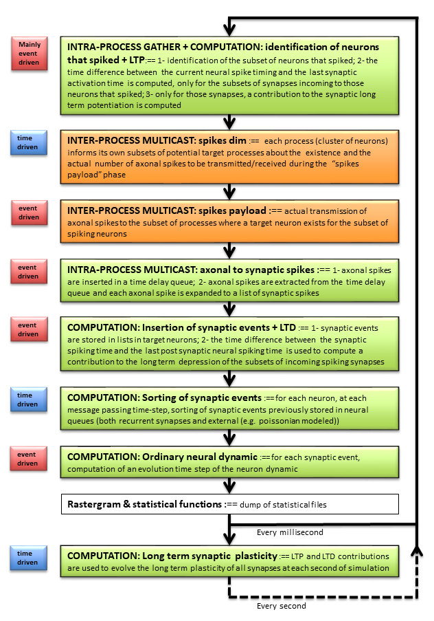
Figure 1: Execution flow of DPSNN simulator. Labels on the left identify event- or time-driven tasks. Orange blocks are used for the inter-processes communication tasks.

II-B Distributed generation of synaptic connections

The described simulation engine exploits its parallelism also during the creation and initialization phase of the network, as detailed in a following section. In a given process, a set of local neurons $i=1,..,N$ projects their set of synapses $j=1,..,M$, toward their target neurons $K^{i,j}$, each synapse characterized by individual delays $D^{i,j}$ and plastic weights $W^{i,j}$. Synaptic efficacies are randomly chosen from Gaussian distributions, while synaptic delays can be generated according to exponential or uniform distribution. The moments of the distributions depend on the source and target populations that each specific synapse interconnects. In addition to recurrent synapses, the system simulates also a number of external synapses: they represent afferent (thalamo-) cortical currents coming from outside the simulated network.

II-C Representation of spiking messages

Spike messages are defined using an Address Event Representation (AER, [28]) including the spiking neuron identifier and the exact spiking time. During simulation, spikes travel from the source to the target neuron. Spikes, whose target neurons belong to the same process, are packed in the axonal spike message.

The arborization of this message is deferred to the target process. Deferring as much as possible the arborization of the “axon” reduces the communication load and unnecessary wait barrier.

To this purpose, preparatory actions are performed during network initialization (performed once at the beginning of the simulation), to reduce the number of active communication channels during the iterative simulation phase.

II-D Initial construction of the connectivity infrastructure

During initialization, each process contributes to create awareness about the subset of processes that should be listened to during next simulation iterations. This knowledge is based on information extracted from the locally constructed matrix of outcoming and incoming synapses. At the end of this construction phase, each “target” process should know about the subset of “source” processes that need to communicate with it, and should have created its database of locally incoming axons and synapses.

A simple implementation of the construction phase can be carried out using two steps. During the first step, each source process informs other processes about the existence of incoming axons and the number of incoming synapses. A single word, the synapse counter, is communicated among pairs of processes. Under MPI, this can be achieved by the MPI_Alltoall() routine. This is performed once, and with a single word payload.

The second construction step transfers the identities of synapses to be created onto each target process. Under MPI, the payload — a list of synapses specific for each pair in the subset of processes to be connected — can be transferred using a call to the MPI_Alltoallv() library function. The number of messages depends on the lateral connectivity range and on the distribution of cortical modules among processes, while the cumulative load is always proportional to the total number of synapses in the system.

The knowledge about the existence of a connection between a pair of processes can be reused to reduce the cost of spiking transmission during the iterations of simulation.

II-E Delivery of spiking messages during the simulation phase

At each iteration, spikes are exchanged between pairs of processes connected by the synaptic matrix. The delivery of spiking messages can be split in two steps, with communications directed toward subsets of decreasing size.

During the first step, single word messages (spike counters) are sent to the subset of potentially connected target processes. On each pair of source-target process subset, the individual spike counter informs about the actual payload — i.e. axonal spikes — to be delivered, or about the absence of spikes to be transmitted. The knowledge of the subset was created during the first step of initialization (see Section II-D).

The second step uses the spiking counter to establish a communication channel only between pairs of processes that actually need to transfer an axonal payload during the current iteration. On MPI, both steps can be implemented using calls to the MPI_Alltoallv() library function.

For two-dimensional grids of neural columns and for their mapping on processes used in this experiment, this implementation proved to be quite efficient, as reported in Section IV, further refined in Section V.

III Neural Network Configuration

III-A Spiking Neuron Model and Synapses

The single-compartment, point-like neurons used in this paper are based on the Leaky Integrate and Fire (LIF) neuron model with spike-frequency adaptation (SFA) due to calcium- and sodium-dependent after-hyperpolarization (AHP) currents [29]. Neuronal dynamics is described by the following equations:

$$\frac{dV}{dt}=\frac{V-E}{\tau_{m}}-g_{c}\frac{c}{C_{m}}+\sum J_{i}\delta(t-t_{i})$$ (1)

$$\frac{dc}{dt}=-\frac{c}{\tau_{c}}$$ (2)

where $V(t)$ represents the membrane potential and $c(t)$ the fatigue variable used to model the SFA as an activity-dependent inhibitory current. $\tau_{m}$ is the membrane characteristic time, $C_{m}$ the membrane capacitance, $E$ the resting potential and $\tau_{c}$ the decay time for the fatigue variable $c$. $g_{c}$, paired with the membrane capacitance, determines the timescales of the coupling of the fatigue (2) and membrane potential (1) equations. For inhibitory neurons, the SFA term is set to zero. Synaptic spikes, reaching the neuron at times $t_{i}$, produce instantaneous membrane potential changes of amplitude $J_{i}$, the weights of activated synapses. When the membrane potential exceeds a threshold $V_{\theta}$, a spike occurs. Thereafter, the membrane potential is reset to $V_{r}$ for a refractory period $\tau_{arp}$, whereas the variable $c$ is increased by the constant amount $\alpha_{c}$.

During the construction phase of the network, recurrent synapses are established between pre- and post-synaptic neurons (see Section III-B). Synaptic efficacies and delays are randomly chosen from probabilistic distributions (see Section II-B).

In addition to the recurrent synapses, the system simulates also a number of external synapses: they represent afferent (thalamo-)cortical currents coming from outside the simulated network, collectively modeled as a Poisson process with a given average spike frequency. The recurrent synapses plus the external synapses yield the number of total synapses afferent to the neuron, referred to as “total equivalent” synapses in the following.

For all the measurements in this work, synaptic plasticity has been disabled, to simplify the comparison between different configurations used in the scaling analysis, ensuring higher stability of the states of the networks.

III-B Cortical Columns and their connectivity

Neurons are organized in cortical modules (mimicking columns), each one composed of 80% excitatory and 20% inhibitory neurons. Modules are assembled in two-dimensional square grids, representing a cortical area slab, with a grid step $\alpha\sim 100$ $\mu$m (inter-columnar spacing). The size of these grids has been varied as per Table I, to perform the scalability experiments here reported.

Each cortical module includes 1240 neurons, while the number of synapses projected by each neuron depends on the implemented connectivity.

The neural network connectivity is set by the user defining the probabilistic connection law between neural populations, spatially located in the two-dimensional grid of cortical modules. Connectivity can be varied according to the simulation needs, leading to configurations with different numbers of synapses per neuron. We adopted the following lateral connectivity rules to evaluate the impact of different inter-module connectivity laws:

• Gaussian connectivity — shorter range and lower number of remote synapses: considering preeminent local connectivity with respect to lateral, the rule used to calculate remote connectivity has been set proportional to $A\cdot exp(\frac{-r^{2}}{2\sigma^{2}}$), with $A=0.05$ and $\sigma=100~{}\mu$m being the lateral spread of the connection probability. The remote connectivity function is similar to that adopted by the [5] model, although with different $A$ and $\sigma$ parameters. In this case only $\sim$20% of the synapses (specifically $\sim$250) are remotely projected and reach modules placed within a short distance, spanning a few steps in the two-dimensional grid of cortical modules. The majority of connections ($\sim$80%) is local to the module.

• Exponential decay connectivity — longer range and higher number of remote synapses: the connectivity rule for remote synapses calculation is proportional to $A\cdot exp(\frac{-r}{\lambda}$), with $A=0.03$ and $\lambda=290~{}\mu$m (the exponential decay constant, in the range of experimental biological values, see e.g. [1]). This turns out into an increased number of remote connections ($\sim$59%), i.e. $\sim$1400 lateral synapses per neuron. It is worth nothing that full biological realism would require to increase the total number of lateral connections above $\sim$4 K synapses/neuron.

For both studied connectivities, a local connection probability of 80% (producing about 990 local synapses) has been adopted. For classical short-range configuration, the dominance of local synapses enables mean-field theory prediction of the dynamical regime of the modules, that perceive the influence of remote modules as small perturbations. In summary, the average number of projected synapses per neuron is $\sim$2390 for the longer-range exponential connectivity while for the Gaussian connectivity is $\sim$1240.

In both systems, a cut-off has been set in the synapses generation, limiting the projection to the subset of modules with connection probability greater than 1/1000. This turns out into stencils of projected connections centered on the source module. A $7\times 7$ stencil is generated in the first case (Gaussian) and a $21\times 21$ in the second case (exponential decay). They are marked in green and orange in Fig. 2.

For each connectivity scheme, measurements were taken on different problem sizes obtained varying the dimension of the grid of modules and, once fixed the problem size, distributing it over a span of MPI processes to evaluate the scaling behaviour.

We selected three grid dimensions: $24\times 24$, $48\times 48$ and $96\times 96$ (see Table I). For a columnar spacing of few hundreds of microns, they can be considered representative of interesting biological cortical slab dimensions. The number of processes over which each network size is distributed varied from a minimum, bounded by memory, and a maximum, bounded by communication (or HPC platform constraints).

Using the Gaussian shorter-range connectivity, an extensive campaign of measures has been conducted, spanning over the three configurations above described. The impact of longer-range exponential decay interconnects has been evaluated on the $24\times 24$ and $48\times 48$ configurations.

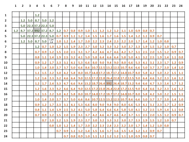
Figure 2: Example of Gaussian (green) and exponential longer-range (orange) connectivity in a grid composed by $24\times 24$ cortical modules: total number of synapses (in thousands) projected by excitatory neurons located in the column marked in grey. Inhibitory neurons project only local connections.

III-C Toward biological modeling

The network size and execution speed reached in the reported scaling experiments makes this engine a valuable candidate tool for the acceleration of large-scale simulations. Here, we report a preliminary example of usage in a specific case of our interest: the modeling of cortical Slow Wave Activity (SWA). To this purpose, we use a three-dimensional variant of the two-dimensional model [30]. The development of the variant and its biological meaning will be presented in a forthcoming publication (preliminary info in [31]). Snapshots of an exemplary propagating wave are reported in Fig. 3. Simulations express delta rhythms, the main feature of SWA, as shown in their power spectral density (Fig. 4). The model includes 2.9 M neurons projecting 3.2 G synapses arranged in a grid of $48\times 48$ cortical modules, spaced at 400 $\mu$m, with a connection probability exponentially decaying with $\lambda$ = 240 $\mu$m. However, the focus of this paper is on the parallel and distributed computing aspects of the engine development and the cost of longer-range lateral connectivity. Papers targeting biological realism are currently under preparation in cooperation with the partners of the WaveScalES experiment in the Human Brain Project.

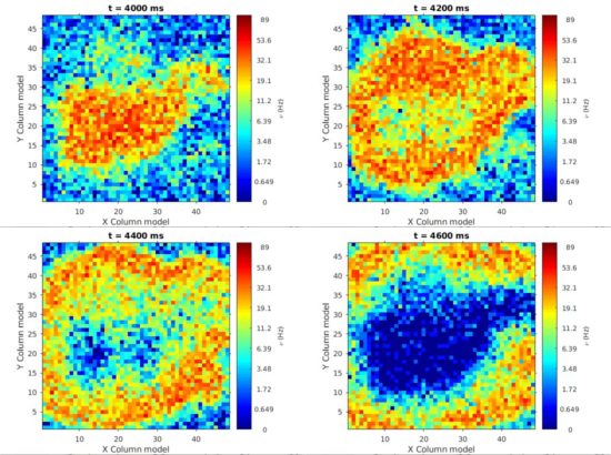
Figure 3: Four snapshot of a slow wave propagating on a $48\times 48$ grid of cortical modules spaced at 400 $\mu$m, with a connection probability exponentially decaying with $\lambda$ = 240 $\mu$m.

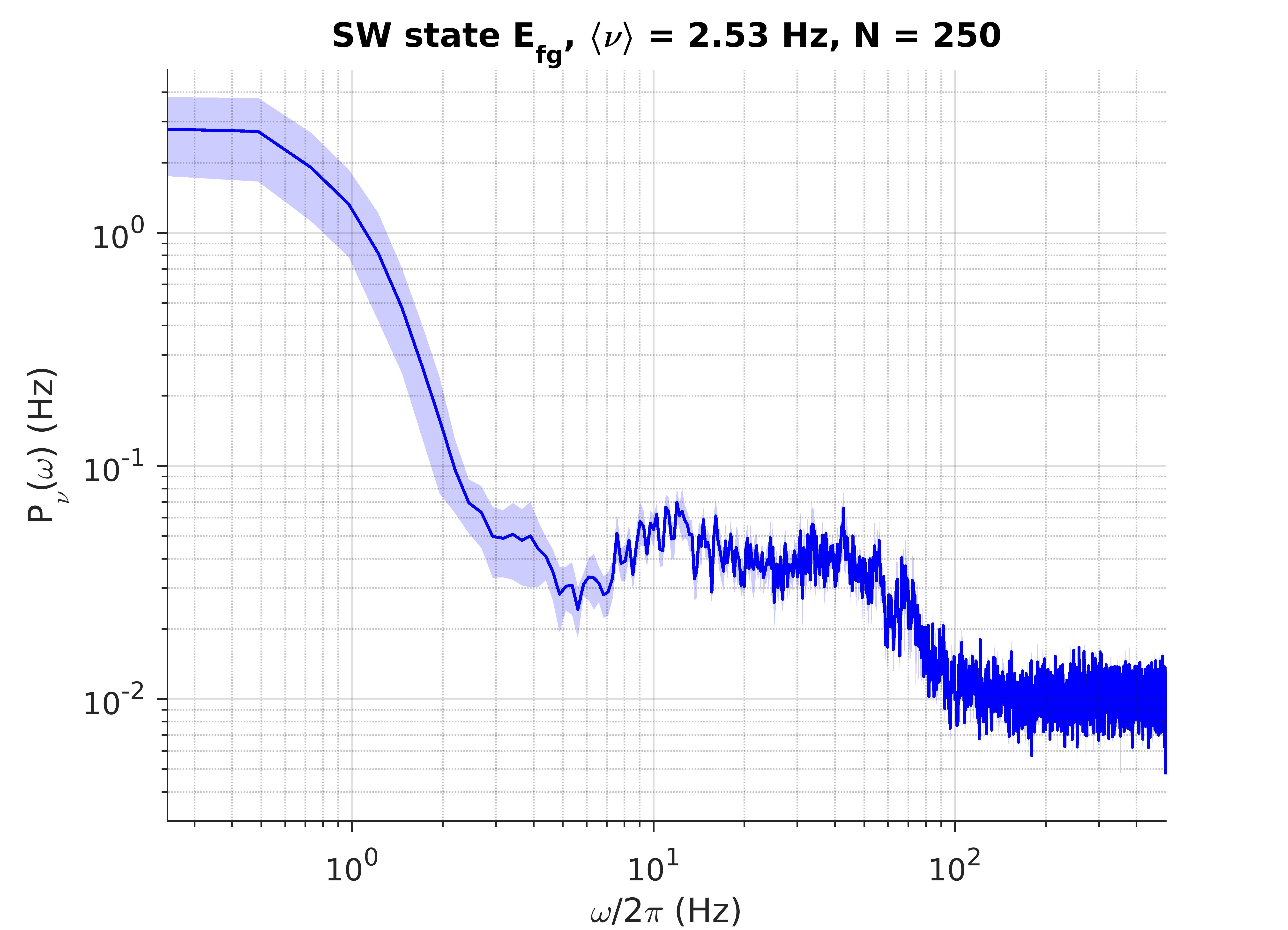
Figure 4: Power spectral density of a population of excitatory neurons showing a high quantity of energy in delta band ($<$ 4 Hz).

III-D Normalized simulation Cost per Synaptic Event

Different network sizes and connectivity models have been used in this scaling analysis. This results in heterogeneous measures of the elapsed time due to different numbers of projected synapses and to the different firing rates of resulting models. For example, the observed firing rate is $\sim$7.5 Hz for the shorter range connectivity, and in the range between 32 and 38 Hz for the longer range one (all other parameters being kept constant). However, a direct comparison is possible converting the execution time into a simulation cost per synaptic event. This normalized cost is computed dividing the elapsed time per simulated second of activity by the number of synapses and by their mean firing rate. In this way, a simple comparison among different simulated configurations is possible: measures from different simulations can be compared on the same plot. Our simulations include two kind of synapses: recurrent — i.e. projected by simulated neurons — and synapses bringing an external stimulus. Summing the number of events generated by recurrent and external synapses, in the following we can normalize the cost to the total number of equivalent synaptic events.

III-E Hardware Platform

We run the simulations on a partition of 64 IBM nodes (1024 cores) of the GALILEO server platform, provided at the CINECA [32] supercomputing center. Each 16-core computational node contains two Intel Xeon Haswell 8-core E5-2630 v3 processors, with a clock of 2.40 GHz. All nodes are interconnected through an InfiniBand network, equipped with 4$\times$ QDR switches. Due to the specific configuration of the server platform, no hyper-threading is allowed. Therefore, in all following measures, the number of cores corresponds exactly to the number of MPI processes launched on a computational node at each execution.

IV Results

TABLE I: Problem sizes for the comparison of simulator performance applied to exponential (longer-range) and Gaussian (shorter-range) connectivity.

Grid	Columns	Neurons	Number of Synapses				MPI Procs
			Gaussian Connectivity		Exponential Connectivity		Min	Max
			Recurrent	Total	Recurrent	Total
$24\times 24$	576	0.7 M	0.9 G	1.2 G	1.5 G	1.8 G	1	64
$48\times 48$	2304	2.9 M	3.5 G	5.0 G	5.9 G	7.4 G	4	256
$96\times 96$	9216	11.4 M	14.2 G	20.4 G	23.4 G	29.6 G	64	1024

IV-A Scaling for shorter range Gaussian connectivity

We collected wall clock execution times simulating different problem sizes (detailed in Table I), spanning from 1 to 1024 MPI processes (or, equivalently, hardware cores). Fig. 5 is about the strong scaling of the execution time per synaptic event. The black dotted line is the ideal scaling: doubling the resources, the execution time should halve. For the $24\times 24$ grid (0.9 G recurrent synapses and 1.2 G total equivalent synapses) the time scales from 275 ns per synaptic event, using a single core, down to 4.09 ns per event using 96 cores. The corresponding speed-up is 67.3 times, losing $\sim$30% compared to the ideal (96 times). For the $48\times 48$ grid (3.5 G recurrent, 5 G equivalent synapses) the speed-up is 54.2 times (ideal 96 times). For the $96\times 96$ grid (14.2 G recurrent/ 20.4 G equivalent synapses) the speed-up is 10.8 times (in this case 16 times would be the ideal).

Figure 6 reports six curves of weak scaling: constant workload per core, while increasing the number of resources and the problem size by up to 16 times. The weak scaling efficiency ranges from 72% (for a workload of 110.7 M synapses per core) down to 54% (when only 13.8 M synapses per core are allocated). Ideal weak scaling (100% efficiency) would produce horizontal lines. Three points per workload are reported: indeed, data have been extracted from the run times of the three configurations $24\times 24$, $48\times 48$, $96\times 96$ used for strong scaling analysis.

In our experience main factors affecting the scaling are collective communications and timing jitter of individual processes due to both operating system interruptions and fluctuations in local workload [18].

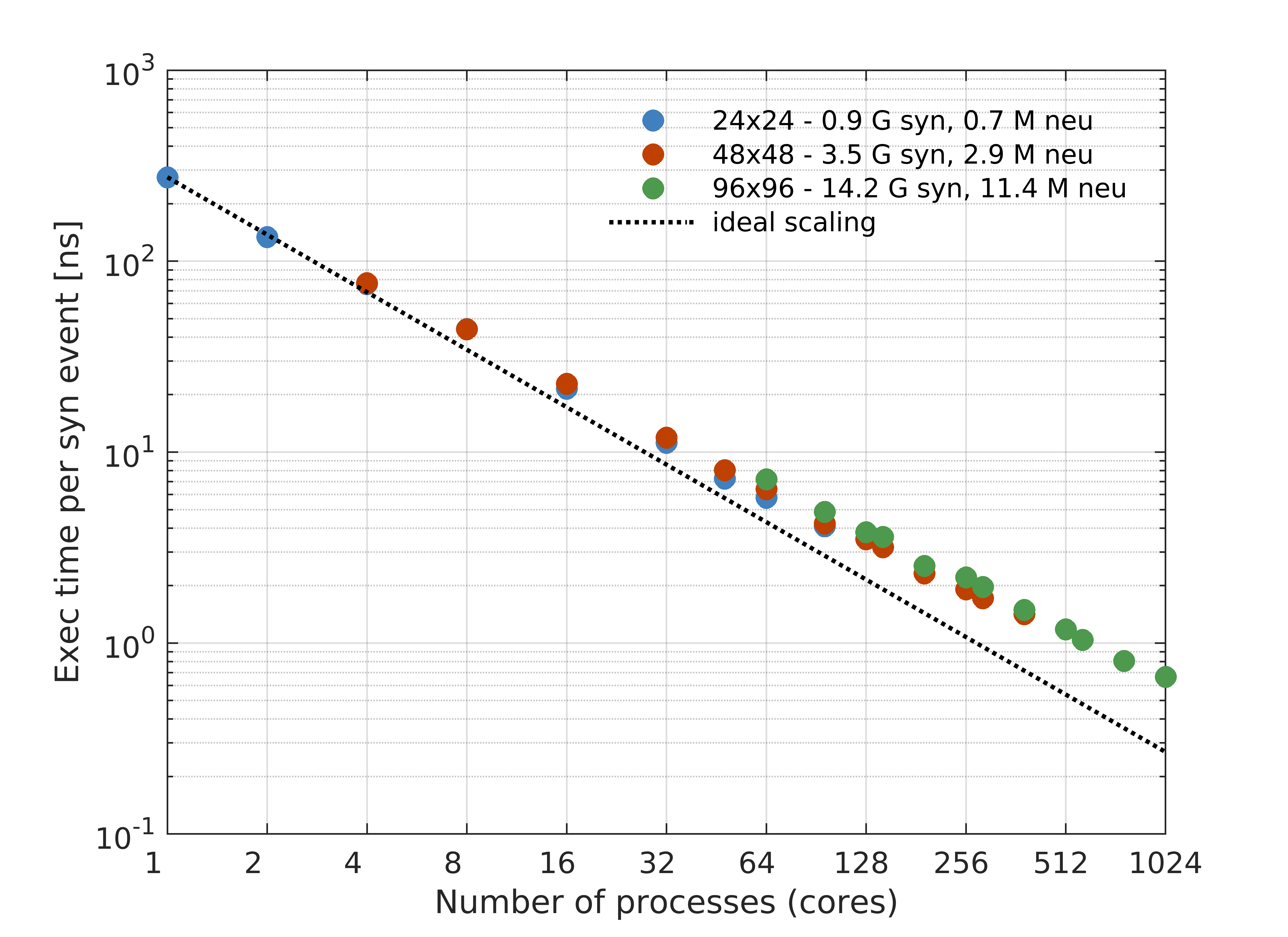
Figure 5: Strong scaling for Gaussian connectivity model: the measures are expressed in elapsed time per equivalent synaptic event.

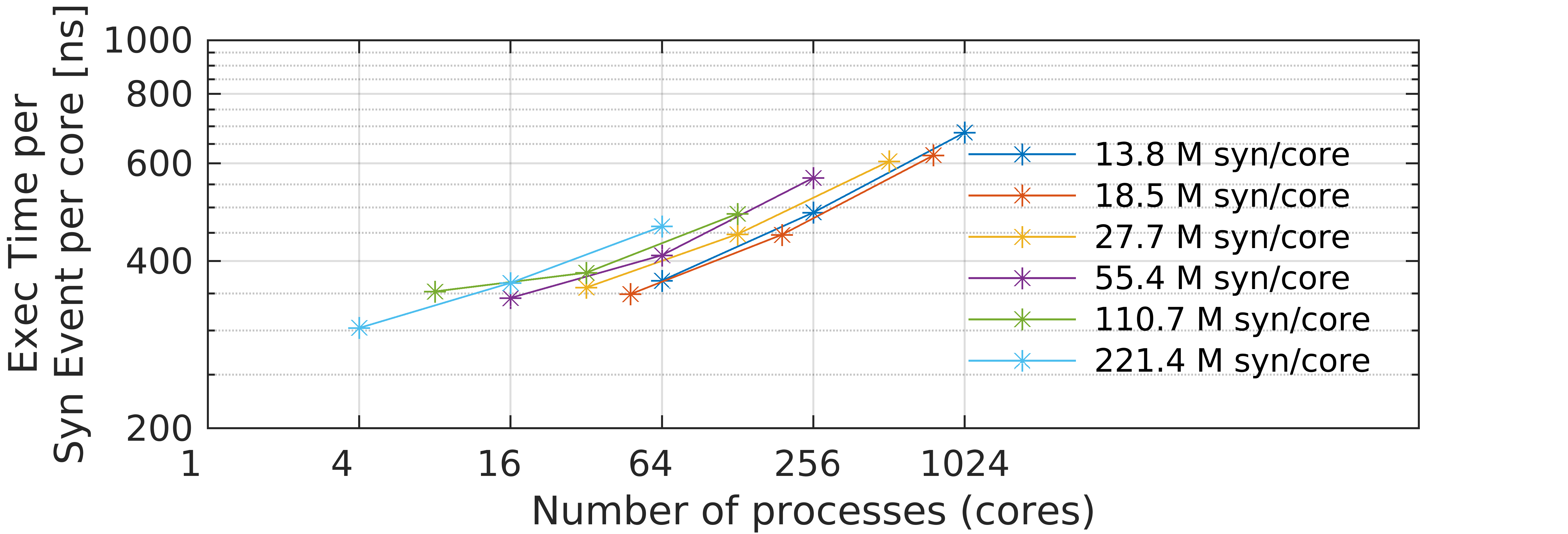
Figure 6: Weak scaling for Gaussian connectivity model.

IV-B Impact of longer range exponential decay connectivity

Fig. 7 compares the impact of shorter and longer lateral connectivity on the strong scaling behaviour. Circles represent measurements for the Gaussian decay while diamonds involve the longer range exponential one.

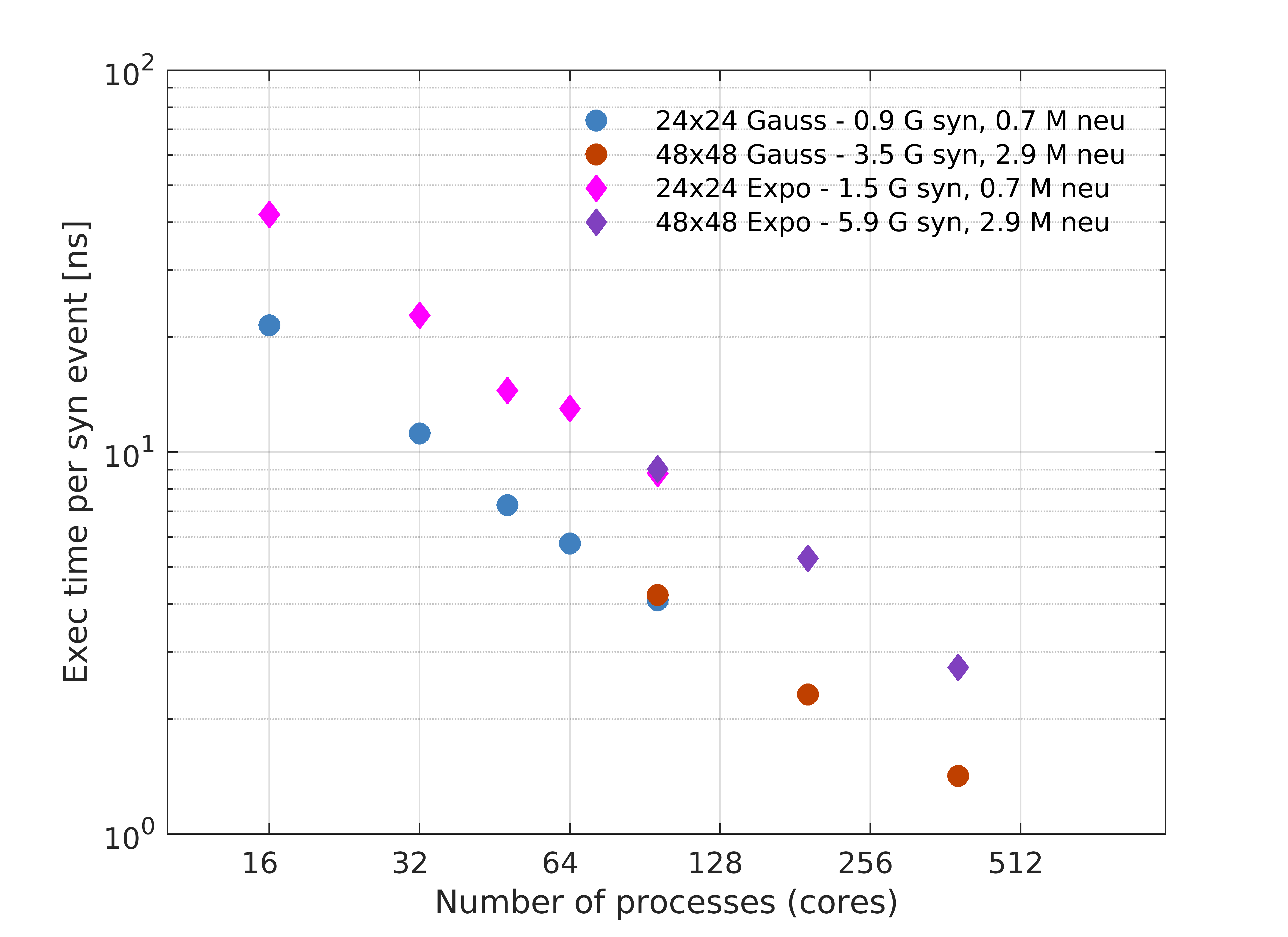
Figure 7: Impact of lateral connectivity: the graph compares the execution time per synaptic event for the configurations with Gaussian connectivity (shorter range, lower number of synapses - circles) and the one with exponential connectivity (longer range, higher number of synapses - diamonds).

The introduction of longer range connectivity increases the simulation cost per synaptic event, with a slow-down between $1.9$ and $2.3$ times, (see Fig. 8). The actual elapsed simulation time increased up to 16.6 times for the exponential longer-range connectivity due to the combined effect produced by: (i) the number of synapses projected by each neuron is higher (by a factor of 1.65), (ii) the firing rates expressed by the model is between 4.3 and 5.0 times higher and (iii) the higher cost of longer range communication and demultiplexing neural spiking messages. Point (iii) should be well estimated by the slow-down of the normalized simulation cost per synaptic event. The execution of longer range connectivity on 96 cores reached about 83% for the $48\times 48$ (5.9 G recurrent synapses) and 79% of the ideal scaling for the $24\times 24$ case (1.5 G recurrent synapses).

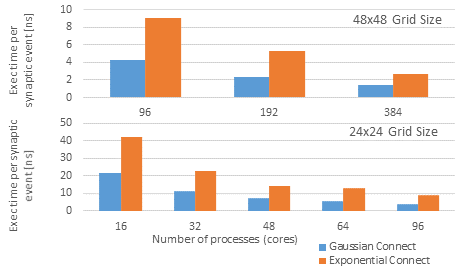
Figure 8: Time per simulated synaptic event increased between 1.9 and 2.3 times on changing the decay of connection probability from the shorter range Gaussian scheme to the longer range exponential one.

IV-C Memory cost per synapse

We measured the total amount of memory allocated and divided it by the number of represented synapses. With no plasticity, each synapse should cost 12 Byte. Peak memory usage is observed at the end of initialization, when each synapse is represented at both the source and target process. Afterwards, memory is released on the source process. The forecast of minimum peak cost is therefore 24 Byte/synapse for static synapses. Fig. 9 shows the maximum memory footprint for different networks sizes and projection ranges, distributed over different numbers of MPI processes. The values are in the range between 26 and 34 Byte per synapse. We observed that the growing cost for higher number of MPI processes is mainly due to the memory allocated by the MPI libraries.

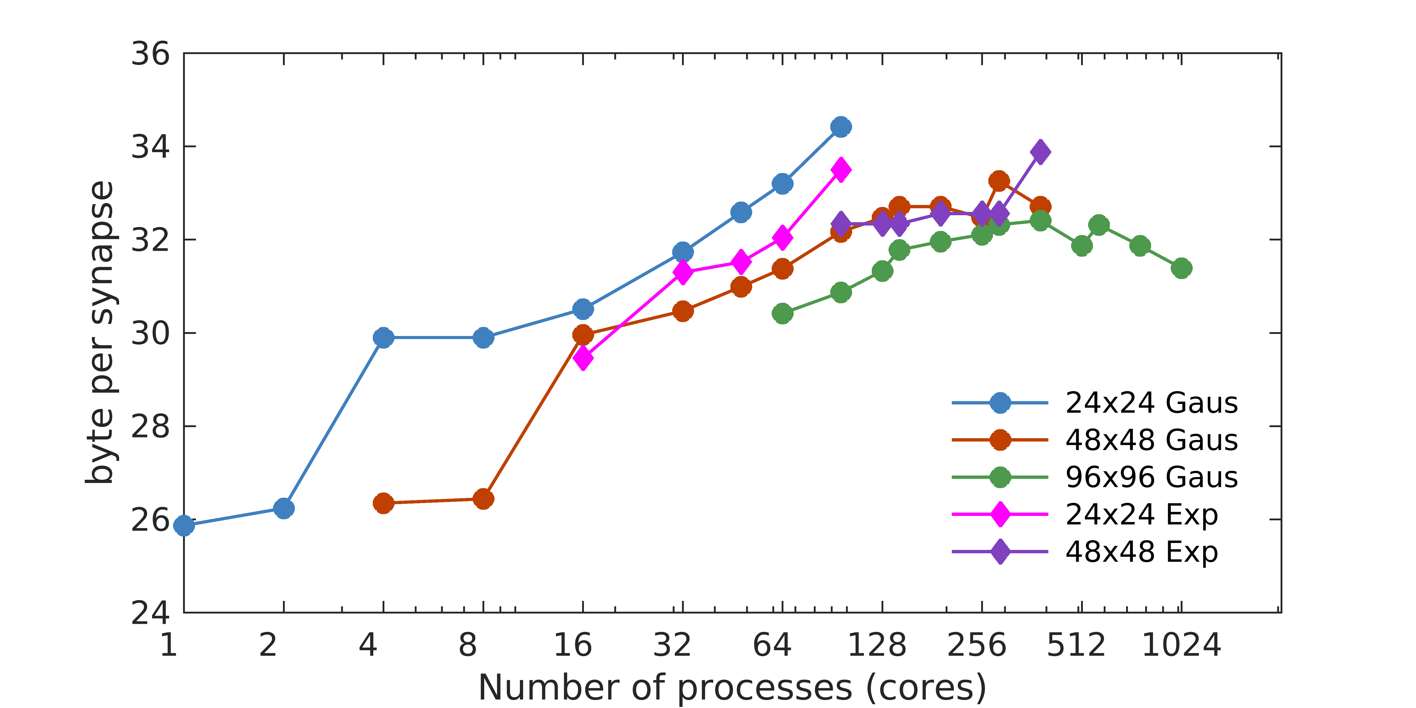
Figure 9: Memory occupation in byte per synapse for different configurations in the two connectivity systems

V Discussion

Recent experimental results suggest the need of supporting long range lateral connectivity in neural simulation of cortical areas — e.g. modeled by simple exponential decay of the connection probability — with layer to layer specific decay constants, in the order of several hundreds of microns. A distributed spiking neural network simulation engine (DPSNN) has been applied to two-dimensional grids of neural columns spaced at 100 $\mu$m connected using two schemes.

The longer-range connectivity model corresponds to an exponential connectivity decay ($\lambda=290~{}\mu$m) and to the projection of approximately $\sim$2390 synapses per neuron. The performance of the engine is compared to that obtained with a shorter range Gaussian decay of connectivity, with a decay constant of the order of the columnar spacing and a lower number of synapses per neuron ($\sim$1240). The impact of longer-range intra-areal exponential connectivity is indeed observable: it increases the simulation cost per synaptic event between 1.9 and 2.3 times compared to traditional shorter-range. The trends of the scaling are quite similar for the two studied connectivities. Notwithstanding the slow-down due to longer range connectivity, the engine demonstrates the ability to simulated large grids of neural columns (up to $96\times 96$), containing a total of up to 11.4 M LIF neurons with spike-frequency adaptation, and representing up to 30 G equivalent synapses on a 1024 core execution platform, with a memory occupation always below 35 Byte/synapse. This is enough to simulate, on clusters of moderate size, cortical slabs with long-range intra-areal lateral interconnect, enabling the modeling of cortical slow waves, a first objective of our team.

A second objective of DPSNN is to support the hardware-software co-design of architectures dedicated to neural simulation. In perspective, we note that more detailed biological simulations of cortical areas could require further extensions of lateral connectivity models and the support of more complex connection motifs at different spatial scales. A further element in future whole brain simulations will be the co-design with white matter inter-areal connectome, which brings sparser connections at system scale. A balance between approaches focalizing on sparse connectivity like [33] and those considering spatial localization (like the one adopted by DPSNN) will have to be carefully addressed for efficient multiscale simulations of the whole brain. The results here presented, combined with previous experiences related to jitter of execution times of individual processes and the impact of collective communications when profiling DPSNN execution on distributed platforms, jointly suggest the utility of designing improved hierarchical communication infrastructures for spiking messages, mechanisms of synchronization of computing nodes and dedicated hardware accelerators. The improvements should consider requirements imposed by biological connectivity, at least for those engines that adopt mapping strategies of neurons and incoming synapses based on spatial contiguity. In such a context, DPSNN can be used to measure the impact of improved designs of execution platforms.

References

- [1] P. Schnepel, A. Kumar, M. Zohar, A. Aertsen, and C. Boucsein, “Physiology and impact of horizontal connections in rat neocortex,” Cerebral Cortex, vol. 25, no. 10, pp. 3818–3835, 2015.
- [2] A. Stepanyants, L. M. Martinez, A. S. Ferecskó, and Z. F. Kisvárday, “The fractions of short- and long-range connections in the visual cortex,” Proceedings of the National Academy of Sciences, vol. 106, no. 9, pp. 3555–3560, 2009.
- [3] C. Boucsein, M. Nawrot, P. Schnepel, and A. Aertsen, “Beyond the cortical column: Abundance and physiology of horizontal connections imply a strong role for inputs from the surround,” Frontiers in Neuroscience, vol. 5, p. 32, 2011.
- [4] A. Schüz, D. Chaimow, D. Liewald, and M. Dortenman, “Quantitative aspects of corticocortical connections: A tracer study in the mouse,” Cerebral Cortex, vol. 16, no. 10, pp. 1474–1486, 2006.
- [5] T. C. Potjans and M. Diesmann, “The cell-type specific cortical microcircuit: Relating structure and activity in a full-scale spiking network model,” Cerebral Cortex, vol. 24, no. 3, pp. 785–806, 2014.
- [6] A. Litwin-Kumar and B. Doiron, “Slow dynamics and high variability in balanced cortical networks with clustered connections,” Nature Neuroscience, vol. 15, p. 1498, 2012.
- [7] E. Gal, M. London, A. Globerson, S. Ramaswamy, M. W. Reimann, E. Muller, H. Markram, and I. Segev, “Rich cell-type-specific network topology in neocortical microcircuitry,” Nature Neuroscience, vol. 20, p. 1004, 2017.
- [8] M.-O. Gewaltig and M. Diesmann, “Nest (neural simulation tool),” Scholarpedia, vol. 2, no. 4, p. 1430, 2007.
- [9] S. Kunkel et al., “Nest 2.12.0,” Mar. 2017.
- [10] R. Brette et al., “Simulation of networks of spiking neurons: A review of tools and strategies,” Journal of Computational Neuroscience, vol. 23, pp. 349–398, Dec 2007.
- [11] M. A. Wilson, U. S. Bhalla, J. D. Uhley, and J. M. Bower, “Genesis: A system for simulating neural networks,” in Advances in Neural Information Processing Systems 1 (D. S. Touretzky, ed.), pp. 485–492, Morgan-Kaufmann, 1989.
- [12] M. Mattia and P. D. Giudice, “Efficient event-driven simulation of large networks of spiking neurons and dynamical synapses,” Neural Computation, vol. 12, pp. 2305–2329, Oct 2000.
- [13] J. M. Nageswaran, N. Dutt, J. L. Krichmar, A. Nicolau, and A. V. Veidenbaum, “A configurable simulation environment for the efficient simulation of large-scale spiking neural networks on graphics processors,” Neural Networks, vol. 22, no. 5, pp. 791 – 800, 2009. Advances in Neural Networks Research: IJCNN2009.
- [14] E. M. Izhikevich and G. M. Edelman, “Large-scale model of mammalian thalamocortical systems,” Proceedings of the National Academy of Sciences, vol. 105, no. 9, pp. 3593–3598, 2008.
- [15] D. S. Modha, R. Ananthanarayanan, S. K. Esser, A. Ndirango, A. J. Sherbondy, and R. Singh, “Cognitive computing,” Commun. ACM, vol. 54, pp. 62–71, Aug. 2011.
- [16] S. B. Furber, D. R. Lester, L. A. Plana, J. D. Garside, E. Painkras, S. Temple, and A. D. Brown, “Overview of the spinnaker system architecture,” IEEE Transactions on Computers, vol. 62, pp. 2454–2467, Dec 2013.
- [17] S. Schmitt et al., “Neuromorphic hardware in the loop: Training a deep spiking network on the brainscales wafer-scale system,” CoRR, vol. abs/1703.01909, 2017.
- [18] P. S. Paolucci et al., “Dynamic many-process applications on many-tile embedded systems and HPC clusters: The EURETILE programming environment and execution platforms,” Journal of Systems Architecture, vol. 69, pp. 29–53, 2016.
- [19] “Euroexa website.” Accessed: 30/Oct/2017.
- [20] M. Katevenis et al., “The ExaNeSt Project: Interconnects, Storage, and Packaging for Exascale Systems,” in 2016 Euromicro Conference on Digital System Design (DSD), pp. 60–67, Aug 2016.
- [21] P. S. Paolucci, R. Ammendola, A. Biagioni, O. Frezza, F. Lo Cicero, A. Lonardo, M. Martinelli, E. Pastorelli, F. Simula, and P. Vicini, “Power, Energy and Speed of Embedded and Server Multi-Cores applied to Distributed Simulation of Spiking Neural Networks: ARM in NVIDIA Tegra vs Intel Xeon quad-cores,” arXiv:1505.03015, June 2015.
- [22] M. Ruiz-Mejias, L. Ciria-Suarez, M. Mattia, and M. V. Sanchez-Vives, “Slow and fast rhythms generated in the cerebral cortex of the anesthetized mouse,” Journal of Neurophysiology, vol. 106, no. 6, pp. 2910–2921, 2011.
- [23] A. Stroh, H. Adelsberger, A. Groh, C. Rühlmann, S. Fischer, A. Schierloh, K. Deisseroth, and A. Konnerth, “Making waves: Initiation and propagation of corticothalamic ca2+ waves in vivo,” Neuron, vol. 77, no. 6, pp. 1136 – 1150, 2013.
- [24] “Human Brain Project.”
- [25] R. Gütig, R. Aharonov, S. Rotter, and H. Sompolinsky, “Learning input correlations through nonlinear temporally asymmetric hebbian plasticity,” Journal of Neuroscience, vol. 23, no. 9, pp. 3697–3714, 2003.
- [26] S. Song, K. D. Miller, and L. F. Abbott, “Competitive hebbian learning through spike-timing-dependent synaptic plasticity,” 2000.
- [27] A. Morrison, C. Mehring, T. Geisel, A. Aertsen, and M. Diesmann, “Advancing the boundaries of high-connectivity network simulation with distributed computing,” Neural Computation, vol. 17, pp. 1776–1801, Aug 2005.
- [28] J. Lazzaro, J. Wawrzynek, M. Mahowald, M. Sivilotti, and D. Gillespie, “Silicon auditory processors as computer peripherals,” pp. 820–827, 1993.
- [29] G. Gigante, M. Mattia, and P. D. Giudice, “Diverse population-bursting modes of adapting spiking neurons,” Phys. Rev. Lett., vol. 98, p. 148101, Apr 2007.
- [30] C. Capone, B. Rebollo, A. Muñoz, X. Illa, P. Del Giudice, M. V. Sanchez-Vives, and M. Mattia, “Slow waves in cortical slices: How spontaneous activity is shaped by laminar structure,” Cerebral Cortex, pp. 1–17, 2017.
- [31] E. Pastorelli, C. Capone, F. Simula, P. Del Giudice, M. Mattia, and P. S. Paolucci, “Distributed large scale simulation of synchronour slow-wave / asynchronous awake-like cortical activity,” 2017. Poster presented at: 5th Annual Human Brain Project Summit, 17-20 October 2017, Glasgow. http://apegate.roma1.infn.it/mediawiki/images/6/62/HBPSummit-DPSNN.pdf.
- [32] GALILEO at CINECA, The Italian Tier-1 cluster for industrial and public research.
- [33] S. Kunkel et al., “Spiking network simulation code for petascale computers,” Frontiers in Neuroinformatics, vol. 8, p. 78, 2014.