Golden Ratio Algorithms for Variational Inequalities

Abstract

The paper presents a fully adaptive algorithm for monotone variational inequalities. In each iteration the method uses two previous iterates for an approximation of the local Lipschitz constant without running a linesearch. Thus, every iteration of the method requires only one evaluation of a monotone operator $F$ and a proximal mapping $g$. The operator $F$ need not be Lipschitz continuous, which also makes the algorithm interesting in the area of composite minimization. The method exhibits an ergodic $O(1/k)$ convergence rate and $R$-linear rate under an error bound condition. We discuss possible applications of the method to fixed point problems as well as its different generalizations.

Keywords. variational inequality $\cdot$ first-order methods $\cdot$ linesearch $\cdot$ saddle point problem $\cdot$ composite minimization $\cdot$ fixed point problem

MSC2010. 47J20, 65K10, 65K15, 65Y20, 90C33

1 Introduction

We are interested in the variational inequality (VI) problem:

$$\text{find }\quad z^{*}\in V\quad\text{ s.t. }\quad\langle F(z^{*}),z-z^{*}\rangle+g(z)-g(z^{*})\geq 0\quad\forall z\in V,$$ (1)

where $V$ is a finite dimensional vector space and we assume that

1. the solution set $S$ of (1) is nonempty;

2. $g\colon V\to(-\infty,+\infty]$ is a proper convex lower semicontinuous (lsc) function;

3. $F\colon\operatorname{dom}g\to V$ is monotone: $\langle F(u)-F(v),u-v\rangle\geq 0$  $\forall u,v\in\operatorname{dom}g$.

The function $g$ can be nonsmooth, and it is very common to consider VI with $g=\delta_{C}$, the indicator function of a closed convex set $C$. In this case (1) reduces to

$$\text{find }\quad z^{*}\in C\quad\text{ s.t. }\quad\langle F(z^{*}),z-z^{*}\rangle\geq 0\quad\forall z\in C,$$ (2)

which is a more widely-studied problem. It is clear that one can rewrite (1) as a monotone inclusion: $0\in(F+\partial g)(x^{*})$. Henceforth, we implicitly assume that we can (relatively simply) compute the resolvent of $\partial g$ (the proximal operator of $g$), that is $(\operatorname{Id}+\partial g)^{-1}$, but cannot do this for $F$, in other words computing the resolvent $(\operatorname{Id}+F)^{-1}$ is prohibitively expensive.

VI is a useful way to reduce many different problems that arise in optimization, PDE, control theory, games theory to a common problem (1). We recommend [29, 21] as excellent references for a broader familiarity with the subject.

As a motivation from the optimization point of view, we present two sources where VI naturally arise. The first example is a convex-concave saddle point problem:

$$\min_{x}\max_{y}\mathcal{L}(x,y):=g_{1}(x)+K(x,y)-g_{2}(y),$$ (3)

where $x\in\mathbb{R}^{n}$, $y\in\mathbb{R}^{m}$, $g_{1}\colon\mathbb{R}^{n}\to(-\infty,+\infty]$, $g_{2}\colon\mathbb{R}^{m}\to(-\infty,+\infty]$ are proper convex lsc functions and $K\colon\operatorname{dom}g_{1}\times\operatorname{dom}g_{2}\to\mathbb{R}$ is a smooth convex-concave function. By writing down the first-order optimality condition, it is easy to see that problem (3) is equivalent to (1) with $F$ and $g$ defined as

$$z=(x,y)\qquad F(z)=\begin{bmatrix}{\nabla_{x}K(x,y)}\\ {-\nabla_{y}K(x,y)}\end{bmatrix}\qquad g(z)=g_{1}(x)+g_{2}(y).$$ (4)

Saddle point problems are ubiquitous in optimization as this is a very convenient way to represent many nonsmooth problems, and this in turn often allows to improve the complexity rates from $O(1/\sqrt{k})$ to $O(1/k)$. Even in the simplest case when $K$ is bilinear form, the saddle point problem is a typical example where the two simplest iterative methods, the forward-backward method and the Arrow-Hurwicz method (see [3]), will not work. Korpelevich in [31] and Popov in [48] resolved this issue by presenting two-step methods that converge for a general monotone $F$. In turn, these two papers gave birth to various improvements and extensions, see [45, 43, 57, 38, 36, 15, 35].

Another important source of VI is a simpler problem of composite minimization

$$\min_{z}J(z):=f(z)+g(z),$$ (5)

where $z\in\mathbb{R}^{n}$, $f\colon\mathbb{R}^{n}\to\mathbb{R}$ is a convex smooth function and $g$ satisfies (C2). This problem is also equivalent to (1) with $F=\nabla f$. On the one hand, it might not be so clever to apply generic VI methods to a specific problem such as (5). Overall, optimization methods have better theoretical convergence rates, and this is natural, since they exploit the fact that $F$ is a potential operator. However, this is only true under the assumption that $\nabla f$ is $L$-Lipschitz continuous. Without such a condition, theoretical rates for the (accelerated) proximal gradient methods do not hold anymore. Recently, there has been a renewed interest in optimization methods for the case with non-Lipschitz $\nabla f$, we refer to [8, 55, 33]. An interesting idea was developed in [8], where the descent lemma was extended to the more general case with Bregman distance. This allows one to obtain a simple method with a fixed stepsize even when $\nabla f$ is not Lipschitz. However, such results are not generic as they depend drastically on problem instances where one can use an appropriate Bregman distance.

For a general VI, even when $F$ is Lipschitz continuous but nonlinear, computing its Lipschitz constant is not an easy task. Moreover, the curvature of $F$ can be quite different, so the stepsizes governed by the global Lipschitz constant will be very conservative. Thus, most practical methods for VI are required to use linesearch — an auxiliary iterative procedure which runs in each iteration of the algorithm until some criterion is satisfied, and it seems this is the only option for the case when $F$ is not Lipschitz. To this end, most known methods for VI with a fixed stepsize have their analogues with linesearch. This is still an active area of research rich in diverse ideas, see [30, 57, 51, 52, 26, 12, 37, 28]. The linesearch can be quite costly in general as it requires computing additional values of $F$ or $\operatorname{prox}_{g}$, or even both in every linesearch iteration. Moreover, the complexity estimates become not so informative, as they only say how many outer iterations one needs to reach the desired accuracy in which the number of linesearch iterations is of course not included.

Contributions. In this paper, our aim is to propose an adaptive algorithm for solving problem (1) with $F$ locally Lipschitz continuous. By adaptive we mean that the method does not require a linesearch to be run, and its stepsizes are computed using current information about the iterates. These stepsizes approximate an inverse local Lipschitz constant of $F$, thus they are separated from zero. Each iteration of the method needs only one evaluation of the proximal operator and one value of $F$. Moreover, the stepsizes are allowed to increase from iteration to iteration. To our knowledge, it is the first adaptive method with such properties. The method is easy to implement and it satisfies all standard rates for monotone VI: ergodic $O(1/k)$ and $R$-linear if the error bound condition holds. In particular, one of possible instances of the proposed algorithm can be given just in a few lines

$$\lambda_{k} =\min\Bigl{\{}\frac{10}{9}\lambda_{k-1},\ \frac{9}{16\lambda_{k-2}}\frac{\|z^{k}-z^{k-1}\|^{2}}{\|F(z^{k})-F(z^{k-1})\|^{2}},\ \bar{\lambda}\Bigr{\}}$$

$$\bar{z}^{k} =\frac{z^{k}+2\bar{z}^{k-1}}{3}$$

$$z^{k+1} =\operatorname{prox}_{\lambda_{k}g}(\bar{z}^{k}-\lambda_{k}F(z^{k})),$$

where $z^{0},z^{1}\in V$, $\bar{z}^{0}=z^{1}$, $\lambda_{0}=\lambda_{-1}>0$, $\bar{\lambda}>0$.

Our approach is to start from the simple case when $F$ is $L$-Lipschitz continuous. For this case, we present the Golden Ratio Algorithm with a fixed stepsize, which is interesting on his own right and gives us an intuition for the more difficult case with dynamic steps. Sect. 2 collects these results. In Sect. 3 we show how one can derive new algorithms for fixed point problems based on the proposed framework. In particular, instead of working with the standard class of nonexpansive operators, we consider a more general class of demi-contractive operators. Sect. 4 collects two extensions of the adaptive Golden Ratio Algorithm. The first proposes an extension of the adaptive algorithm enhanced by two auxiliary metrics. Although it is simple theoretically, it is nevertheless still very important in applications, where it is preferable to use different weights for different coordinates. For the second extension we do not need monotonicity of $F$, but instead we require that the Minty variational inequality associated with (1) has a solution. In Sect. 5 we illustrate the performance of the method for several problems including the aforementioned nonmonotone case. Finally, Sect. 6 concludes the paper by presenting several directions for further research.

Preliminaries. Let $V$ be a finite-dimensional vector space equipped with inner product $\langle\cdot,\cdot\rangle$ and norm $\|\cdot\|=\sqrt{\langle\cdot,\cdot\rangle}$. For a lsc function $g\colon V\to(-\infty,+\infty]$ by $\operatorname{dom}g$ we denote the domain of $g$, i.e., the set $\{x\colon g(x)<+\infty\}$. Given a closed convex set $C$, $P_{C}$ stands for the metric projection onto $C$, $\delta_{C}$ denotes the indicator function of $C$ and $\operatorname{dist}(x,C)$ the distance from $x$ to $C$, that is $\operatorname{dist}(x,C)=\|P_{C}x-x\|$. The proximal operator $\operatorname{prox}_{g}$ for a proper lsc convex function $g\colon V\to(-\infty,+\infty]$ is defined as $\operatorname{prox}_{g}(z)=\operatorname{argmin}_{x}\{g(x)+\frac{1}{2}\|x-z\|^{2}\}$. The following characteristic property (prox-inequality) will be frequently used:

$$\bar{x}=\operatorname{prox}_{g}z\quad\Leftrightarrow\quad\langle\bar{x}-z,x-\bar{x}\rangle\geq g(\bar{x})-g(x)\quad\forall x\in V.$$ (6)

A simple identity important in our analysis is

$$\|\alpha a+(1-\alpha)b\|^{2}=\alpha\|a\|^{2}+(1-\alpha)\|b\|^{2}-\alpha(1-\alpha)\|a-b\|^{2}\ \ \forall a,b\in V\ \forall\alpha\in\mathbb{R}.$$ (7)

The following important lemma will simplify the proofs of the main theorems.

Lemma 1.

Let $(z^{k})\subset V$ be a bounded sequence and suppose $\lim_{k\to\infty}\|z^{k}-z\|$ exists whenever $z$ is a cluster point of $(z^{k})$. Then $(z^{k})$ is convergent.

Proof.

Assume that $u,v$ are two arbitrary cluster points of $(z^{k})$. From

$$\langle z^{k}-u,u-v\rangle=\frac{1}{2}\|z^{k}-v\|^{2}-\frac{1}{2}\|z^{k}-u\|^{2}-\frac{1}{2}\|u-v\|^{2}$$ (8)

we see that there exists $\lim_{k\to\infty}\langle z^{k}-u,u-v\rangle$. Assume now that $z^{k_{i}}\to u$ and $z^{k_{j}}\to v$. Then one can observe that

$$0=\lim_{i\to\infty}\langle z^{k_{i}}-u,u-v\rangle=\lim_{j\to\infty}\langle z^{k_{j}}-u,v-u\rangle=\|v-u\|^{2}$$ (9)

and hence, $u=v$. Since $u,v$ were arbitrary, we can conclude that $(z^{k})$ converges to some element in $V$. ∎

2 Golden Ratio Algorithms

Let $\varphi=\frac{\sqrt{5}+1}{2}$ be the golden ratio, that is $\varphi^{2}=1+\varphi$. The proposed Golden RAtio ALgorithm (GRAAL for short) reads as a simple recursion:

$$\bar{z}^{k} =\frac{(\varphi-1)z^{k}+\bar{z}^{k-1}}{\varphi}$$ (10)

$$z^{k+1} =\operatorname{prox}_{\lambda g}(\bar{z}^{k}-\lambda F(z^{k})).$$

Theorem 1.

Suppose that $F\colon\operatorname{dom}g\to V$ is $L$–Lipschitz and conditions (C1)–(C3) are satisfied. Let $z^{1},\bar{z}^{0}\in V$ be arbitrary and $\lambda\in(0,\frac{\varphi}{2L}]$. Then $(z^{k})$, $(\bar{z}^{k})$, generated by (10), converge to a solution of (1).

Proof.

By the prox-inequality (6) we have

$$\langle z^{k+1}-\bar{z}^{k}+\lambda F(z^{k}),z-z^{k+1}\rangle\geq\lambda(g(z^{k+1})-g(z))\quad\forall z\in V$$ (11)

and

$$\langle z^{k}-\bar{z}^{k-1}+\lambda F(z^{k-1}),z^{k+1}-z^{k}\rangle\geq\lambda(g(z^{k})-g(z^{k+1})).$$ (12)

Note that $z^{k}-\bar{z}^{k-1}=\frac{1+\varphi}{\varphi}(z^{k}-\bar{z}^{k})=\varphi(z^{k}-\bar{z}^{k})$. Hence, we can rewrite (12) as

$$\langle\varphi(z^{k}-\bar{z}^{k})+\lambda F(z^{k-1}),z^{k+1}-z^{k}\rangle\geq\lambda(g(z^{k})-g(z^{k+1})).$$ (13)

Summation of (11) and (13) yields

$$\langle z^{k+1}-\bar{z}^{k},z-z^{k+1}\rangle+\varphi\langle z^{k}-\bar{z}^{k},z^{k+1}-z^{k}\rangle+\lambda\langle F(z^{k}),z-z^{k}\rangle\\ +\lambda\langle F(z^{k})-F(z^{k-1}),z^{k}-z^{k+1}\rangle\geq\lambda(g(z^{k})-g(z)).$$ (14)

Expressing the first two terms in (14) through norms, we arrive at

$$\|z^{k+1}-z\|^{2}\leq\|\bar{z}^{k}-z\|^{2} -\|z^{k+1}-\bar{z}^{k}\|^{2}+2\lambda\langle F(z^{k})-F(z^{k-1}),z^{k}-z^{k+1}\rangle$$

$$+\varphi(\|z^{k+1}-\bar{z}^{k}\|^{2}-\|z^{k+1}-z^{k}\|^{2}-\|z^{k}-\bar{z}^{k}\|^{2})$$

$$-2\lambda\bigl{(}\langle F(z^{k}),z^{k}-z\rangle+g(z^{k})-g(z)\bigr{)}.$$ (15)

Choose $z=z^{*}\in S$. By (C3), the rightmost term in (2) is nonnegative:

$$\langle F(z^{k}),z^{k}-z^{*}\rangle+g(z^{k})-g(z^{*})\geq\langle F(z^{*}),z^{k}-z^{*}\rangle+g(z^{k})-g(z^{*})\geq 0.$$ (16)

By (7) and $z^{k+1}=(1+\varphi)\bar{z}^{k+1}-\varphi\bar{z}^{k}$ we have

$$\|z^{k+1}-z^{*}\|^{2} =(1+\varphi)\|\bar{z}^{k+1}-z^{*}\|^{2}-\varphi\|\bar{z}^{k}-z^{*}\|^{2}+\varphi(1+\varphi)\|\bar{z}^{k+1}-\bar{z}^{k}\|^{2}$$

$$=(1+\varphi)\|\bar{z}^{k+1}-z^{*}\|^{2}-\varphi\|\bar{z}^{k}-z^{*}\|^{2}+\frac{1}{\varphi}\|z^{k+1}-\bar{z}^{k}\|^{2}.$$ (17)

Combining (2) and (16) with (2), we deduce

$$(1+\varphi)\|\bar{z}^{k+1}-z^{*}\|^{2}\leq(1 +\varphi)\|\bar{z}^{k}-z^{*}\|^{2}-\varphi(\|z^{k+1}-z^{k}\|^{2}+\|z^{k}-\bar{z}^{k}\|^{2})$$

$$+2\lambda\|F(z^{k})-F(z^{k-1})\|\|z^{k}-z^{k+1}\|.$$ (18)

From $\lambda\leq\frac{\varphi}{2L}$ it follows that

$$2\lambda\|F(z^{k})-F(z^{k-1})\|\|z^{k+1}-z^{k}\|\leq\frac{\varphi}{2}(\|z^{k}-z^{k-1}\|^{2}+\|z^{k+1}-z^{k}\|^{2}),$$ (19)

which finally leads to

$$(1+\varphi)\|\bar{z}^{k+1}-z^{*}\|^{2}+\frac{\varphi}{2}\|z^{k+1}-z^{k}\|^{2}\leq(1+\varphi)\|\bar{z}^{k}-z^{*}\|^{2}+\frac{\varphi}{2}\|z^{k}-z^{k-1}\|^{2}-\varphi\|z^{k}-\bar{z}^{k}\|^{2}.$$ (20)

From (20) we have that $\bigl{(}(1+\varphi)\|\bar{z}^{k+1}-z^{*}\|^{2}+\frac{\varphi}{2}\|z^{k+1}-z^{k}\|^{2}\bigr{)}$ is bounded and so is $(\bar{z}^{k})$, and $\lim_{k\to\infty}\|z^{k}-\bar{z}^{k}\|=0$. Hence, $(z^{k})$ has at least one cluster point. By definition of $\bar{z}^{k}$, $z^{k+1}-\bar{z}^{k}=\varphi(z^{k+1}-\bar{z}^{k+1})\to 0$ and, hence, $z^{k+1}-z^{k}\to 0$ as well. Taking the limit in (11) (going to the subsequences if needed) and using (C2), we prove that all cluster points of $(z^{k})$ (and thus, of $(\bar{z}^{k})$) belong to $S$. From (20) one can see that the sequence $\bigl{(}(1+\varphi)\|\bar{z}^{k}-z^{*}\|^{2}+\frac{\varphi}{2}\|z^{k}-z^{k-1}\|\bigr{)}$ is non-increasing and, hence, it is convergent. As $\lim_{k\to\infty}\|z^{k}-z^{k-1}\|=0$, there must exist $\lim_{k\to\infty}\|\bar{z}^{k}-z^{*}\|$. Since $z^{*}$ is an arbitrary point in $S$, from Lemma 1 it follows that $(\bar{z}^{k})$ and $(z^{k})$ converge to a point in $S$. ∎

Notice that the constant $\varphi$ is chosen not arbitrary, but as the largest constant $c$ that satisfies $\frac{1}{c}\geq c-1$ in order to get rid of the term $\|z^{k+1}-\bar{z}^{k}\|^{2}$ in (2). It is interesting to compare the proposed GRAAL with the reflected projected (proximal) gradient method [36]. At a first glance, they are quite similar: both need one $F$ and one $\operatorname{prox}_{g}$ per iteration. The advantage of the former, however, is that $F$ is computed at $z^{k}$, which is always feasible $z^{k}\in\operatorname{dom}g$, due to the properties of the proximal operator. In the reflected projected (proximal) gradient method $F$ is computed at $2z^{k}-z^{k-1}$ which might be infeasible. Sometimes, as it will be illustrated in Sect. 5, this can be important.

2.1 Adaptive Golden Ratio Algorithm

In this section we introduce our fully adaptive algorithm. The algorithm preserves the same computational cost per iteration as (10) (i.e., no linesearch) and the stepsizes approximate an inverse local Lipschitz constant of $F$. Furthermore, for our purposes, the locally Lipschitz continuity of $F$ is sufficient. The algorithm, which we call the adaptive Golden Ratio Algorithm (aGRAAL), is presented as Alg. 1. For simplicity, we adopt the convention $\frac{0}{0}=+\infty$.

Algorithm 1 Adaptive Golden Ratio Algorithm

  Input: Choose $z^{0},z^{1}\in V$, $\lambda_{0}>0$, $\phi\in(1,\varphi]$, $\bar{\lambda}>0$. Set $\bar{z}^{0}=z^{1}$, $\theta_{0}=1$, $\rho=\frac{1}{\phi}+\frac{1}{\phi^{2}}$.

  For $k\geq 1$ do

   1. Find the stepsize:

$$\lambda_{k}=\min\Bigl{\{}\rho\lambda_{k-1},\ \frac{\phi\theta_{k-1}}{4\lambda_{k-1}}\frac{\|z^{k}-z^{k-1}\|^{2}}{\|F(z^{k})-F(z^{k-1})\|^{2}},\ \bar{\lambda}\Bigr{\}}$$ (21)

   2. Compute the next iterates:

$$\bar{z}^{k} =\frac{(\phi-1)z^{k}+\bar{z}^{k-1}}{\phi}$$ (22)

$$z^{k+1} =\operatorname{prox}_{\lambda_{k}g}(\bar{z}^{k}-\lambda_{k}F(z^{k})).$$ (23)

   3. Update: $\theta_{k}=\dfrac{\lambda_{k}}{\lambda_{k-1}}\phi$.

Notice that in the $k$-th iteration we need only to compute $F(z^{k})$ once and reuse the already computed value $F(z^{k-1})$. The constant $\bar{\lambda}$ in (21) is given only to ensure that $(\lambda_{k})$ is bounded. Hence, it makes sense to choose $\bar{\lambda}$ quite large. Although $\lambda_{0}$ can be arbitrary from the theoretical point of view, from (21) it is clear that $\lambda_{0}$ will influence further steps, so in practice we do not want to take it too small or too large. The simplest way is to choose $z^{0}$ as a small perturbation of $z^{1}$ and take $\lambda_{0}=\frac{\|z^{1}-z^{0}\|}{\|F(z^{1})-F(z^{0})\|}$. This gives us an approximation of the local inverse Lipschitz constant of $F$ at $z^{1}$.

As one can see from Alg. 1, for $\phi<\varphi$ one has $\rho>1$ and hence, $\lambda_{k}$ can be larger than $\lambda_{k-1}$. This is probably the most important feature of the proposed algorithm. When $F$ is Lipschitz, there are some other methods without linesearch that do not require to know the Lipschitz constant, e.g.,[58]. However, such methods use nonincreasing stepsizes, which is rather restrictive.

Condition (21) leads to two key estimations. First, one has $\lambda_{k}\leq\lambda_{k-1}(\frac{1}{\phi}+\frac{1}{\phi^{2}})$, which in turn implies $\theta_{k}-1-\frac{1}{\phi}\leq 0$. Second, from $\frac{\phi\theta_{k-1}}{\lambda_{k-1}}=\frac{\theta_{k}\theta_{k-1}}{\lambda_{k}}$ one can derive

$$\lambda_{k}^{2}\|F(z^{k})-F(z^{k-1})\|^{2}\leq\frac{\theta_{k}\theta_{k-1}}{4}\|z^{k}-z^{k-1}\|^{2}.$$ (24)

Alg. 1 is quite generic, and in order to simplify it we can predefine some of the constants. Let $\phi=\frac{3}{2}$. Then $\rho=\frac{10}{9}$ and as $\theta_{k-1}=\frac{\lambda_{k-1}}{\lambda_{k-2}}\phi$, we have $\frac{\phi\theta_{k-1}}{4\lambda_{k-1}}=\frac{9}{16\lambda_{k-2}}$. It is easy to see that with such choice of constants, Alg. 1 reduces to the one we presented in the introduction.

Lemma 2.

Suppose that $F\colon\operatorname{dom}g\to V$ is locally Lipschitz continuous. If the sequence $(z^{k})$ generated by Alg. 1 is bounded, then both $(\lambda_{k})$ and $(\theta_{k})$ are bounded and separated from $0$.

Proof.

It is obvious that $(\lambda_{k})$ is bounded. Let us prove by induction that it is separated from $0$. As $(z^{k})$ is bounded there exists some $L>0$ such that $\|F(z^{k})-F(z^{k-1})\|\leq L\|z^{k}-z^{k-1}\|$. Moreover, we can take $L$ large enough to ensure that $\lambda_{i}\geq\frac{\phi^{2}}{4L^{2}\bar{\lambda}}$ for $i=0,1$. Now suppose that for all $i=0,\dots k-1$, $\lambda_{i}\geq\frac{\phi^{2}}{4L^{2}\bar{\lambda}}$. Then we have either $\lambda_{k}=\rho\lambda_{k-1}\geq\lambda_{k-1}\geq\frac{\phi^{2}}{4L^{2}\bar{\lambda}}$ or

$$\lambda_{k}=\frac{\phi^{2}}{4\lambda_{k-2}}\frac{\|z^{k}-z^{k-1}\|^{2}}{\|F(z^{k})-F(z^{k-1})\|^{2}}\geq\frac{\phi^{2}}{4\lambda_{k-2}L^{2}}\geq\frac{\phi^{2}}{4L^{2}\bar{\lambda}}.$$ (25)

Hence, in both cases $\lambda_{k}\geq\frac{\phi^{2}}{4L^{2}\bar{\lambda}}$. The claim that $(\theta_{k})$ is bounded and separated from $0$ now follows immediately. ∎

Define the bifunction $\Psi(u,v):=\langle F(u),v-u\rangle+g(v)-g(u)$. It is clear that (1) is equivalent to the following equilibrium problem: find $z^{*}\in V$ such that $\Psi(z^{*},z)\geq 0$ $\forall z\in V$. Notice that for any fixed $z$, the function $\Psi(z,\cdot)$ is convex.

Theorem 2.

Suppose that $F\colon\operatorname{dom}g\to V$ is locally Lipschitz and conditions (C1)–(C3) are satisfied. Then $(z^{k})$ and $(\bar{z}^{k})$, generated by Alg. 1, converge to a solution of (1).

Proof.

Let $z\in V$ be arbitrary. By the prox-inequality (6) we have

$$\langle z^{k+1}-\bar{z}^{k}+\lambda_{k}F(z^{k}),z-z^{k+1}\rangle \geq\lambda_{k}(g(z^{k+1})-g(z))$$ (26)

$$\langle z^{k}-\bar{z}^{k-1}+\lambda_{k-1}F(z^{k-1}),z^{k+1}-z^{k}\rangle \geq\lambda_{k-1}(g(z^{k})-g(z^{k+1}))\ .$$ (27)

Multiplying (27) by $\frac{\lambda_{k}}{\lambda_{k-1}}\geq 0$ and using that $\frac{\lambda_{k}}{\lambda_{k-1}}(z^{k}-\bar{z}^{k-1})=\theta_{k}(z^{k}-\bar{z}^{k})$, we obtain

$$\langle\theta_{k}(z^{k}-\bar{z}^{k})+\lambda_{k}F(z^{k-1}),z^{k+1}-z^{k}\rangle\geq\lambda_{k}(g(z^{k})-g(z^{k+1})).$$ (28)

Summation of (26) and (28) gives us

$$\langle z^{k+1}-\bar{z}^{k},z-z^{k+1}\rangle +\theta_{k}\langle z^{k}-\bar{z}^{k},z^{k+1}-z^{k}\rangle+\lambda_{k}\langle F(z^{k})-F(z^{k-1}),z^{k}-z^{k+1}\rangle$$

$$\geq\lambda_{k}\langle F(z^{k}),z^{k}-z\rangle+\lambda_{k}(g(z^{k})-g(z))$$

$$\geq\lambda_{k}[\langle F(z),z^{k}-z\rangle+g(z^{k})-g(z)]=\lambda_{k}\Psi(z,z^{k}).$$ (29)

Expressing the first two terms in (2.1) through norms, we derive

$$\|z^{k+1}-z\|^{2}\leq\|\bar{z}^{k}-z\|^{2} -\|z^{k+1}-\bar{z}^{k}\|^{2}+2\lambda_{k}\langle F(z^{k})-F(z^{k-1}),z^{k}-z^{k+1}\rangle$$

$$+\theta_{k}\bigl{(}\|z^{k+1}-\bar{z}^{k}\|^{2}-\|z^{k+1}-z^{k}\|^{2}-\|z^{k}-\bar{z}^{k}\|^{2}\bigr{)}-2\lambda_{k}\Psi(z,z^{k}).$$ (30)

Similarly to (2), we have

$$\|z^{k+1}-z\|^{2}=\frac{\phi}{\phi-1}\|\bar{z}^{k+1}-z\|^{2}-\frac{1}{\phi-1}\|\bar{z}^{k}-z\|^{2}+\frac{1}{\phi}\|z^{k+1}-\bar{z}^{k}\|^{2}.$$ (31)

Combining this with (2.1), we obtain

$$\frac{\phi}{\phi-1}\|\bar{z}^{k+1}-z\|^{2}\leq\frac{\phi}{\phi-1}\|\bar{z}^{k}-z\|^{2}+\bigl{(}\theta_{k}-1-\frac{1}{\phi}\bigr{)}\|z^{k+1}-\bar{z}^{k}\|^{2}-2\lambda_{k}\Psi(z,z^{k})\\ -\theta_{k}\bigl{(}\|z^{k+1}-z^{k}\|^{2}+\|z^{k}-\bar{z}^{k}\|^{2}\bigr{)}+2\lambda_{k}\langle F(z^{k})-F(z^{k-1}),z^{k}-z^{k+1}\rangle.$$ (32)

Recall that $\theta_{k}\leq 1+\frac{1}{\phi}$. Using (24), the rightmost term in (32) can be estimated as

$$2\lambda_{k}\langle F(z^{k})-F(z^{k-1}),z^{k}-z^{k+1}\rangle\leq 2\lambda_{k}\|F(z^{k})-F(z^{k-1})\|\|z^{k}-z^{k+1}\|\\ \leq\sqrt{\theta_{k}\theta_{k-1}}\|z^{k}-z^{k-1}\|\|z^{k}-z^{k+1}\|\leq\frac{\theta_{k}}{2}\|z^{k+1}-z^{k}\|^{2}+\frac{\theta_{k-1}}{2}\|z^{k}-z^{k-1}\|^{2}.$$ (33)

Applying the obtained estimation to (32), we deduce

$$\frac{\phi}{\phi-1}\|\bar{z}^{k+1}-z\|^{2}+\frac{\theta_{k}}{2}\|z^{k+1}-z^{k}\|^{2}+2\lambda_{k}\Psi(z,z^{k})\\ \leq\frac{\phi}{\phi-1}\|\bar{z}^{k}-z\|^{2}+\frac{\theta_{k-1}}{2}\|z^{k}-z^{k-1}\|^{2}-\theta_{k}\|z^{k}-\bar{z}^{k}\|^{2}.$$ (34)

Iterating the above inequality, we derive

$$\frac{\phi}{\phi-1}\|\bar{z}^{k+1}-z\|^{2}+\frac{\theta_{k}}{2}\|z^{k+1}-z^{k}\|^{2}+\sum_{i=2}^{k}\theta_{i}\|z^{i}-\bar{z}^{i}\|^{2}+2\sum_{i=1}^{k}\lambda_{k}\Psi(z,z^{k})\\ \leq\frac{\phi}{\phi-1}\|\bar{z}^{2}-z\|^{2}+\frac{\theta_{1}}{2}\|z^{2}-z^{1}\|^{2}-\theta_{2}\|z^{2}-\bar{z}^{2}\|^{2}+2\lambda_{1}\Psi(z,z^{1}).$$ (35)

Let $z=z^{*}\in S$. Then the last term in the left-hand side of (35) is nonnegative. This yields that $(\bar{z}^{k})$, and hence $(z^{k})$, is bounded, and $\theta_{k}\|z^{k}-\bar{z}^{k}\|\to 0$. Now we can apply Lemma 2 to deduce that $\lambda_{k}\geq\frac{\phi^{2}}{4L^{2}\bar{\lambda}}$ and $(\theta_{k})$ is separated from zero. Thus, $\lim_{k\to\infty}\|z^{k}-\bar{z}^{k}\|=0$, which implies $z^{k}-\bar{z}^{k-1}\to 0$ and thus, also $z^{k+1}-z^{k}\to 0$. Let us show that all cluster points of $(z^{k})$ and $(\bar{z}^{k})$ belong to $S$. This is proved in the standard way. Let $(k_{i})$ be a subsequence such that $z^{k_{i}}\to\tilde{z}$ and $\lambda_{k_{i}}\to\lambda>0$ as $i\to\infty$. Clearly, $z^{k_{i}+1}\to\tilde{z}$ and $\bar{z}^{k_{i}}\to\tilde{z}$ as well. Then consider (26) indexed by $k_{i}$ instead of $k$. Taking the limit as $i\to\infty$ in it and using (C2), we obtain

$$\lambda\langle F(\tilde{z}),z-\tilde{z}\rangle\geq\lambda(g(\tilde{z})-g(z))\quad\forall z\in V.$$ (36)

Hence, $\tilde{z}\in S$. From (34) one can see that the sequence $\bigl{(}\frac{\phi}{\phi-1}\|\bar{z}^{k}-z\|^{2}+\frac{\theta_{k-1}}{2}\|z^{k}-z^{k-1}\|^{2}\bigr{)}$ is nonincreasing, hence $\lim_{k\to\infty}\|\bar{z}^{k}-z\|$ exists. As $z\in S$ is arbitrary, from Lemma 1 it follows that sequences $(\bar{z}^{k})$, $(z^{k})$ converge to some element in $S$. This completes the proof. ∎

Remark 1.

For a variational inequality in the form (2), condition (C3) can be relaxed to the following

1. $\langle F(z),z-\bar{z}\rangle\geq 0\quad\forall z\in C\quad\forall\bar{z}\in S$.

This condition, used for example in [51], is weaker than the standard monotonicity assumption (C3) or pseudomonotonicity assumption:

$$\langle F(v),u-v\rangle\geq 0\quad\Longrightarrow\quad\langle F(u),u-v\rangle\geq 0.$$ (37)

It is straightforward to see that Theorems 1, 2 hold under (C4). In fact, in the proof of the theorems, we choose $z=z^{*}\in S$ only to ensure that $\Psi(z^{*},z^{k})\geq 0$. However, it is sufficient to show that the first left-hand side in (2.1) is nonnegative. But for $z=z^{*}\in S$ this is true, since by (C4), $\langle F(z^{k}),z^{k}-z^{*}\rangle\geq 0$.

2.2 Ergodic convergence

It is known that many algorithms for monotone VI (or for more specific convex-concave saddle point problems) exhibit an $O(1/k)$ rate of convergence, see, for instance, [43, 45, 39, 17], where such an ergodic rate was established. Moreover, Nemirovski has shown in [44, 43] that this rate is optimal. In this section we prove the same result for our algorithm. When the set $\operatorname{dom}g$ is bounded establishing such a rate is a simple task for most methods, including aGRAAL, however the case when $\operatorname{dom}g$ is unbounded has to be examined more carefully. To deal with it, we use the notion of the restricted merit function, first proposed in [45].

Choose any $\tilde{x}\in\operatorname{dom}g$ and $r>0$. Let $U=\operatorname{dom}g\cap\mathbb{B}(\tilde{x},r)$, where $\mathbb{B}(\tilde{x},r)$ denotes a closed ball with center $\tilde{x}$ and radius $r$. Recall the bifunction we work with $\Psi(u,v):=\langle F(u),v-u\rangle+g(v)-g(u)$. The restricted merit (dual gap) function is defined as

$$e_{r}(v)=\max_{u\in U}\Psi(u,v)\qquad\forall v\in V.$$ (38)

From [45] we have the following fact:

Lemma 3.

The function $e_{r}$ is well defined and convex on $V$. For any $x\in U$, $e_{r}(x)\geq 0$. If $x^{*}\in U$ is a solution to (1), then $e_{r}(x^{*})=0$. Conversely, if $e_{r}(\hat{x})=0$ for some $\hat{x}$ with $\|\hat{x}-\tilde{x}\|<r$, then $\hat{x}$ is a solution of (1).

Proof.

The proof is almost identical to Lemma 1 in [45]. The only difference is that we have to consider VI (1) with a general $g$ instead of $\delta_{C}$. ∎

Now we can obtain something meaningful. Since $F$ is continuous and $g$ is lsc, there exist some constant $M>0$ that majorizes the right-hand side of (35) for all $z\in U$. From this follows that $\sum_{i=1}^{k}\lambda_{i}\Psi(z,z^{i})\leq M$ for all $z\in U$ (we ignore the constant $2$ before the sum). Let $Z^{k}$ be the ergodic sequence: $Z^{k}=\frac{\sum_{i=1}^{k}\lambda_{i}z_{i}}{\sum_{i=1}^{k}\lambda_{i}}$. Then using convexity of $\Psi(z,\cdot)$, we obtain

$$e_{r}(Z^{k})=\max_{z\in U}\Psi(z,Z^{k})\leq\frac{1}{\sum_{i=1}^{k}{\lambda_{i}}}\max_{z\in U}\bigl{(}\sum_{i=1}^{k}\Psi(z,z^{i})\bigr{)}\leq\frac{M}{\sum_{i=1}^{k}{\lambda_{i}}}.$$ (39)

Taking into account that $(\lambda_{k})$ is separated from zero, we obtain the $O(1/k)$ convergence rate for the ergodic sequence $(Z^{k})$.

Remark 2.

For the case of the composite minimization problem (5), instead of using the merit function it is simpler to use the energy residual: $J(z^{k})-J(z^{*})$. For this we need to use in (2.1) that

$$\lambda_{k}\langle F(z^{k}),z^{k}-z\rangle+\lambda_{k}(g(z^{k})-g(z)) \geq\lambda_{k}[f(z^{k})-f(z)+g(z^{k})-g(z)]$$

$$=\lambda_{k}(J(z^{k})-J(z)).$$ (40)

In this way, we may proceed analogously to obtain

$$\min_{i=1,\dots,k}(J(z^{i})-J(z^{*}))\leq\frac{M}{\sum_{i=1}^{k}{\lambda_{i}}}\quad\text{and}\quad J(Z^{k})-J(z^{*})\leq\frac{M}{\sum_{i=1}^{k}{\lambda_{i}}}.$$ (41)

2.3 Linear convergence

For many VI methods it is possible to derive a linear convergence rate under some additional assumptions. The most general tool for that is the use of error bounds. For a survey of error bounds, we refer the reader to [46] and for their applications to the VI algorithms to [56, 50].

Let us briefly recall the terminology associated with linear convergence. Suppose that $(u^{k})\subset V$ is a sequence that converges to $u\in V$. We say that convergence is $Q$-linear, if there is $q\in(0,1)$ such that $\|u^{k+1}-u\|<q\|u^{k}-u\|$ for all $k$ large enough. We also say that convergence is $R$-linear, if for all $k$ large enough, $\|u^{k}-u\|\leq\gamma_{k}$ and $(\gamma_{k})$ converges $Q$-linearly to zero.

Let us fix some $\lambda>0$ and define the natural residual $r(z,\lambda):=z-\operatorname{prox}_{\lambda g}(z-\lambda F(z))$. Evidently, $z\in S$ if and only if $r(z,\lambda)=0$. We say that problem (1) satisfies an error bound condition if there exist positive constants $\mu$ and $\eta$ such that

$$\operatorname{dist}(z,S)\leq\mu\|r(z,\lambda)\|\qquad\forall x\quad\text{with}\quad\|r(z,\lambda)\|\leq\eta.$$ (42)

The function $\lambda\mapsto\|r(z,\lambda)\|$ is nondecreasing and $\lambda\mapsto\frac{\|r(z,\lambda)\|}{\lambda}$is nonincreasing (see [21, Proposition 10.3.6]), and thus all natural residuals $r(\cdot,\lambda)$ are equivalent. Hence the choice of $\lambda$ in the above definition is not essential. No doubt, it is not an easy task to decide whether (42) holds for a particular problem. Several examples are known, see for instance [50, 21] and it is still an important and active area of research.

In the analysis below we are not interested in sharp constants, but rather in showing the linear convergence for $(z^{k})$. This will allow us to keep the presentation simpler. For the same reason we assume that $F$ is $L$-Lipschitz continuous.

Choose any $\lambda>0$ such that $\lambda_{k}\geq\lambda$ for all $k$. Without loss of generality, we assume that $\lambda$ is the same as in (42). As $\lambda\mapsto\|r(\cdot,\lambda)\|$ is nondecreasing and $\operatorname{prox}_{\lambda_{k}g}$ is nonexpansive, using the triangle inequality, we obtain

$$\|r(\bar{z}^{k},\lambda)\| \leq\|r(\bar{z}^{k},\lambda_{k})\|=\|\operatorname{prox}_{\lambda_{k}g}(\bar{z}^{k}-\lambda_{k}F(\bar{z}^{k}))-\bar{z}^{k}\|$$

$$\leq\|\operatorname{prox}_{\lambda_{k}g}(\bar{z}^{k}-\lambda_{k}F(\bar{z}^{k}))-\operatorname{prox}_{\lambda_{k}g}(\bar{z}^{k}-\lambda_{k}F(z^{k}))\|+\|z^{k+1}-\bar{z}^{k}\|$$

$$\leq\lambda_{k}L\|z^{k}-\bar{z}^{k}\|+\|z^{k+1}-z^{k}\|+\|z^{k}-\bar{z}^{k}\|$$

$$=(1+\lambda_{k}L)\|z^{k}-\bar{z}^{k}\|+\|z^{k+1}-z^{k}\|,$$ (43)

From this it follows that

$$\|r(\bar{z}^{k},\lambda)\|^{2}\leq 2(1+\lambda_{k}L)^{2}\|z^{k}-\bar{z}^{k}\|^{2}+2\|z^{k+1}-z^{k}\|^{2}.$$ (44)

Let $\beta=\frac{\phi}{\phi-1}$. If $(\theta_{k})$ is separated from zero, then the above inequality ensures that for any $z^{k},\bar{z}^{k}$ and $\varepsilon\in(0,1)$ there exists $m\in(0,1)$ such that

$$m\beta\mu^{2}\|r(\bar{z}^{k},\lambda)\|^{2}\leq\theta_{k}\|z^{k}-\bar{z}^{k}\|^{2}+\theta_{k}\frac{\varepsilon}{2}\|z^{k+1}-z^{k}\|^{2}.$$ (45)

The presence of so many constants in (45) will be clear later. In order to proceed, we have to modify Alg. 1. Now instead of (21), we choose the stepsize by

$$\lambda_{k}=\min\Bigl{\{}\rho\lambda_{k-1},\ \frac{\phi\delta\theta_{k-1}}{4\lambda_{k-1}}\frac{\|z^{k}-z^{k-1}\|^{2}}{\|F(z^{k})-F(z^{k-1})\|^{2}},\ \bar{\lambda}\Bigr{\}},\qquad\delta\in(0,1).$$ (46)

This modification basically means that we slightly bound the stepsize. However, this is not crucial for the steps, as we can choose $\delta$ arbitrary close to one. An argument completely analogous to that in the proof of Lemma 2 (up to the factor $\delta$) shows that both $(\lambda_{k})$ and $(\theta_{k})$ are bounded and separated from zero. This confirms correctness of our arguments about $(\lambda_{k})$ and $(\theta_{k})$ in (2.3) and (44). It should be also obvious that Alg. 1 with (46) instead of (21) has the same convergence properties, since (33) — the only place where this modification plays some role — will be still valid. For any $\delta\in(0,1)$ there exist $\varepsilon\in(0,1)$ and $m\in(0,1)$ such that $\delta=(1-\varepsilon)(1-m)$ and (45) is fulfilled for any $z^{k},\bar{z}^{k}$. Now using (46), one can derive a refined version of (33):

$$2\lambda_{k} \langle F(z^{k})-F(z^{k-1}),z^{k}-z^{k+1}\rangle\leq 2\lambda_{k}\|F(z^{k})-F(z^{k-1})\|\|z^{k}-z^{k+1}\|$$

$$\leq\sqrt{\delta\theta_{k}\theta_{k-1}}\|z^{k}-z^{k-1}\|\|z^{k}-z^{k+1}\|$$

$$\leq\frac{(1-\varepsilon)\theta_{k}}{2}\|z^{k+1}-z^{k}\|^{2}+\frac{(1-m)\theta_{k-1}}{2}\|z^{k}-z^{k-1}\|^{2}.$$ (47)

With this inequality, instead of (34), for $z=z^{*}\in S$ we have

$$\beta\|\bar{z}^{k+1}-z^{*}\|^{2}+\frac{\theta_{k}}{2}\|z^{k+1}-z^{k}\|^{2}+2\lambda_{k}\Psi(z^{*},z^{k})$$

$$\leq\ \beta\|\bar{z}^{k}-z^{*}\|^{2}+\frac{\theta_{k-1}(1-m)}{2}\|z^{k}-z^{k-1}\|^{2}-\theta_{k}\|z^{k}-\bar{z}^{k}\|^{2}-\theta_{k}\frac{\varepsilon}{2}\|z^{k+1}-z^{k}\|^{2}$$

$$\leq\ \beta\|\bar{z}^{k}-z^{*}\|^{2}+\frac{\theta_{k-1}(1-m)}{2}\|z^{k}-z^{k-1}\|^{2}-m\beta\mu^{2}\|r(\bar{z}^{k},\lambda)\|^{2},$$ (48)

where in the last inequality we have used (45). As $(\bar{z}^{k})$ converges to a solution, $r(\bar{z}^{k},\lambda)$ goes to $0$, and hence $\|r(\bar{z}^{k},\lambda)\|\leq\eta$ for all $k\geq k_{0}$. Setting $z^{*}=P_{S}(\bar{z}^{k})$ in (2.3) and using (42) and that $\Psi(z^{*},z^{k})\geq 0$, we obtain

$$\beta\operatorname{dist}(\bar{z}^{k+1},S)^{2} +\frac{\theta_{k}}{2}\|z^{k+1}-z^{k}\|^{2}\leq\beta\|\bar{z}^{k+1}-z^{*}\|^{2}+\frac{\theta_{k}}{2}\|z^{k+1}-z^{k}\|^{2}$$

$$\leq(1-m)\bigl{(}\beta\operatorname{dist}(\bar{z}^{k},S)^{2}+\frac{\theta_{k-1}}{2}\|z^{k}-z^{k-1}\|^{2}\bigr{)}.$$ (49)

From this the $Q$-linear rate of convergence for the sequence $\bigl{(}\operatorname{dist}(\bar{z}^{k},S)^{2}+\frac{\theta_{k-1}}{2}\|z^{k}-z^{k-1}\|^{2}\bigr{)}$ follows. Since $(\theta_{k})$ is separated from zero, we conclude that $\|z^{k}-z^{k-1}\|$ converges $R$-linearly and this immediately implies that the sequence $(z^{k})$ converges $R$-linearly. We summarize the obtained result in the following statement.

Theorem 3.

Suppose that conditions (C1)–(C3) are satisfied, $F\colon\operatorname{dom}g\to V$ is $L$–Lipschitz and the error bound (42) holds. Then $(z^{k})$, generated by Alg. 1 with (46) instead of (21), converges to a solution of (1) at least $R$-linearly.

3 Fixed point algorithms

Although in general it is a very standard way to formulate a VI (1) as a fixed point equation $x=\operatorname{prox}_{g}(x-F(x))$, sometimes other way around might also be beneficial. In this section we show how one can apply general algorithms for VI to find a fixed point of some operator $T\colon V\to V$. Clearly, any fixed point equation $x=Tx$ is equivalent to the equation $F(x)=0$ with $F=\operatorname{Id}-T$. The latter problem is of course a particular instance of (1) with $g\equiv 0$. Hence, we can work under the assumptions of Remark 1.

By $\operatorname{Fix}T$ we denote the fixed point set of the operator $T$. Although, with a slight abuse of notation, we will not use brackets for the argument of $T$ (this is common in the fixed point literature), but we continue doing that for the argument of $F$.

We are interested in the following classes of operators:

1. Firmly-nonexpansive:

   $$\|Tx-Ty\|^{2}\leq\|x-y\|^{2}-\|(x-Tx)-(y-Ty)\|^{2}\quad\forall x,y\in V.$$

2. Nonexpansive:

   $$\|Tx-Ty\|\leq\|x-y\|\quad\forall x,y\in V.$$

3. Quasi-nonexpansive:

   $$\|Tx-\bar{x}\|\leq\|x-\bar{x}\|\quad\forall x\in V,\forall\bar{x}\in\operatorname{Fix}T.$$

4. Pseudo-contractive:

   $$\|Tx-Ty\|^{2}\leq\|x-y\|^{2}+\|(x-Tx)-(y-Ty)\|^{2}\quad\forall x,y\in V.$$

5. Demi-contractive:

   $$\|Tx-\bar{x}\|^{2}\leq\|x-\bar{x}\|^{2}+\|x-Tx\|^{2}\quad\forall x\in V,\forall\bar{x}\in\operatorname{Fix}T.$$

We have the following obvious relations

$$\begin{cases}(a)\subset(b)\subset(c)\subset(e)\\ (a)\subset(b)\subset(d)\subset(e).\end{cases}$$ (50)

Therefore, (e) is the most general class of the aforementioned operators. Sometimes in the literature [49, 13, 42] the authors consider operators that satisfy a more restrictive condition

$$\|Tx-\bar{x}\|^{2}\leq\|x-\bar{x}\|^{2}+\rho\|x-Tx\|^{2}\quad\forall x\in V,\forall\bar{x}\in\operatorname{Fix}T\quad\rho\in[0,1]$$ (51)

and call them $\rho$–demi-contractive for $\rho\in[0,1)$ and hemi-contractive for $\rho=1$. We consider only the most general case with $\rho=1$, but still for simplicity will call them as demi-contractive. It is also tempting to call the class (e) as quasi-pseudocontractive by keeping the analogy between (b) and (c), but this tends to be a bit confusing due to “quasi-pseudo”. Notice that for the case $\rho<1$ in (51), one can consider a relaxed operator $S=\rho\operatorname{Id}+(1-\rho)T$. It is easy to see that $S$ belongs to the class (c) and $\operatorname{Fix}S=\operatorname{Fix}T$. However, with $\rho=1$, the situation becomes much more difficult.

When $T$ belongs to (a) or (b), the standard way to find a fixed point of $T$ is by applying the celebrated Krasnoselskii-Mann scheme (see e.g. [10]): $x^{k+1}=\alpha x^{k}+(1-\alpha)Tx^{k}$, where $\alpha\in(0,1)$. The same method can be applied when $T$ is in class (c), but to the averaged operator $S=\beta\operatorname{Id}+(1-\beta)T$, $\beta\in(0,1)$, instead of $T$. However, things become more difficult when we consider broader classes of operators. In particular, Ishikawa in [25] proposed an iterative algorithm when $T$ is Lipschitz continuous and pseudo-contractive. However, its convergence requires a compactness assumption, which is already too restrictive. Moreover, the convergence is rather slow, since the scheme uses some auxiliary slowly vanishing sequence (as in the subgradient method), also the scheme uses two evaluations of $T$ per iteration. Later, this scheme was extended in [49] to the case when $T$ is Lipschitz continuous and demi-contractive but with the same assumptions as above.

Obviously, one can rewrite condition (e) as

$$\langle Tx-x,\bar{x}-x\rangle\geq 0\quad\forall x\in V,\,\forall\bar{x}\in\operatorname{Fix}T,$$ (52)

which means that the angle between vectors $Tx-x$ and $\bar{x}-x$ must always be nonobtuse.

We know that $T$ is pseudo-contractive if and only if $F$ is monotone [10, Example 20.8]. It is not more difficult to check that $T$ is demi-contractive if and only if $F$ satisfies (C4). In fact, in this case $S=\operatorname{Fix}T$, thus, (52) and (C4) are equivalent: $\langle F(x),x-\bar{x}\rangle=\langle x-Tx,x-\bar{x}\rangle\geq 0$. The latter observation allows one to obtain a simple way to find a fixed point of a demi-contractive operator $T$. In particular, in order to find a fixed point of $T$, one can apply the aGRAAL. Moreover, since in our case $g\equiv 0$ and $\operatorname{prox}_{g}=\operatorname{Id}$, (23) simplifies to

$$x^{k+1}=\bar{x}^{k}-\lambda_{k}F(x^{k}) =(\bar{x}^{k}-\lambda_{k}x^{k})+\lambda_{k}Tx^{k}$$

$$=\bigl{(}\frac{\phi-1}{\phi}-\lambda_{k}\bigr{)}x^{k}+\frac{1}{\phi}\bar{x}^{k-1}+\lambda_{k}Tx^{k}.$$ (53)

From the above it follows:

Theorem 4.

Let $T\colon V\to V$ be locally Lipschitz and demi-contractive operator. Define $F=\operatorname{Id}-T$. Then the sequence $(x^{k})$ defined by aGRAAL with (3) instead of (23) converges to a fixed point of $T$.

Proof.

Since $F=\operatorname{Id}-T$ is obviously locally Lipschitz, the proof is an immediate application of Theorem 2. ∎

Remark 3.

The obtained theorem is interesting not only for the very general class of demi-contractive operators, but for a more limited class of non-expansive operators. The scheme (3) requires roughly the same amount of computations as the Krasnoselskii-Mann algorithm, but the former method defines $\lambda_{k}$ from the local properties of $T$, and hence, depending on the problem, it can be much larger than $1$. Recently, there appeared some papers on speeding-up the Krasnoselskii-Mann (KM) scheme for nonexpansive operators [54, 22]. The first paper proposes a simple linesearch in order to accelerate KM. However, as it is common for all linesearch procedures, each inner iteration requires an evaluation of the operator $T$, which in the general case can eliminate all advantages of it. The second paper considers a more general framework, inspired by Newton methods. However, its convergence guarantees are more restrictive.

The demi-contractive property can be useful when we want to analyze the convergence of the iterative algorithm $x^{k+1}=Tx^{k}$ for some operator $T$. It might happen that we cannot prove that $(x^{k})$ is Fejér monotone w.r.t. $\operatorname{Fix}T$, but instead we can only show that $\|x^{k+1}-\bar{x}\|^{2}\leq\|x^{k}-\bar{x}\|^{2}+\|x^{k+1}-x^{k}\|^{2}$ for all $\bar{x}\in\operatorname{Fix}T$. This estimation guarantees that $T$ is demi-contractive and hence one can apply Theorem 4 to obtain a sequence that converges to $\operatorname{Fix}T$.

Finally, we can relax condition in (e) to the following

$$\|Tx-P_{S}x\|^{2}\leq\|x-P_{S}x\|^{2}+\|x-Tx\|^{2}\quad\forall x\in V,$$ (54)

which in turn is equivalent to $\langle F(x),x-P_{S}x\rangle\geq 0$ for all $x\in V$. For instance, (54) might arise when we know that $F=\operatorname{Id}-T$ satisfies a global error bound condition

$$\operatorname{dist}(x,S)\leq\mu\|F(x)\|=\mu\|x-Tx\|\qquad\forall x\in V,$$ (55)

and it holds that

$$\|Tx-\bar{x}\|^{2}\leq(1+\varepsilon)\|x-\bar{x}\|^{2}\qquad\forall x\in V\,\,\forall\bar{x}\in S,$$ (56)

where $\varepsilon>0$ is some constant. One can easily show that (54) follows from (55) and (56), whenever $\varepsilon<\frac{1}{\mu^{2}}$. The proof of convergence for aGRAAL with this new condition will be almost the same: in the $k$-th iteration instead of using arbitrary $x^{*}\in S$, we have to set $x^{*}=P_{S}x^{k}$. Of course, the global error bound condition (55) is too restrictive and is difficult to verify [21, Chapter 6]. On the other hand, property (56) is very attractive: it is often the case that for some iterative scheme one can only show (56), which is not enough to proceed further with standard arguments like the Krasnoselskii-Mann theorem or Banach contraction principle. We believe it might be an interesting avenue for further research to consider the above settings with $\mu$ and $\varepsilon$ dependent on $x$ in order to eliminate the limitation of (55). Condition (56) also relates to the recent work [34] where the generalization of nonexpansive operators for multivalued case was considered.

4 Generalizations

This section deals with two generalizations. First, we present aGRAAL in a general metric settings. Although this extension should be straightforward for most readers, we present it to make this work self-contained. Next, by revisiting the proof of convergence for aGRAAL we relax the monotonicity condition to a new one and discuss its consequences.

4.1 aGRAAL with different metrics

Throughout section 2 we have been working in standard Euclidean metric $\langle\cdot,\cdot\rangle$ and assumed that $F$ is monotone with respect to it. There are at least two possible generalizations of how one can incorporate some metric into Alg. 1. Firstly, the given operator $F$ may not be monotone in metric $\langle\cdot,\cdot\rangle$, but it is so in $\langle\cdot,\cdot\rangle_{P}$, induced by some symmetric positive definite operator $P$. For example, the generalized proximal method $z^{k+1}=(\operatorname{Id}+P^{-1}G)^{-1}z^{k}$ for some monotone operator $G$ gives us the operator $T=(\operatorname{Id}+P^{-1}G)^{-1}$ which is nonexpansive in metric $\langle\cdot,\cdot\rangle_{P}$, and hence $F=\operatorname{Id}-T$ is monotone in that metric but is not so in $\langle\cdot,\cdot\rangle$. This is an important example, as it incorporates many popular methods: ADMM, Douglas-Rachford, PDHG, etc. Secondly, it is often desirable to consider an auxiliary metric $\langle\cdot,\cdot\rangle_{M}$, induced by a symmetric positive definite operator $M$, that will enforce faster convergence. For instance, for saddle point problems, one may give different weights for primal and dual variables, in this case one will consider some diagonal scaling matrix $M$. The standard analysis of aGRAAL (and this is common for other known methods) does not take into account that $F$ is derived from a saddle point problem; it treats the operator $F$ as a black box, and just use one stepsize $\lambda$ for both primal and dual variables. For example, the primal-dual hybrid gradient algorithm [16], which is a very popular method for solving saddle point problems with a linear operator, uses different steps $\tau$ and $\sigma$ for primal and dual variables; and the performance of this method drastically depends on the choice of these constants. This should be kept in mind when one applies aGRAAL for such problems.

Another possibility is if we already work in metric $\langle\cdot,\cdot\rangle_{P}$, then a good choice of the matrix $M$ can eliminate some undesirable computations, like computing the proximal operator in metric $\langle\cdot,\cdot\rangle_{P}$. Of course, the idea to incorporate a specific metric to the VI algorithm for a faster convergence is not new and was considered, for example, in [52, 19, 24]. Our goal is to show that the framework of GRAAL can easily adjust to these new settings.

Let $M,P\colon V\to V$ be symmetric positive definite operators. We consider two norms induces by $M$ and $P$ respectively

$$\|z\|_{M}:=\sqrt{\langle z,z\rangle_{M}}=\langle Mz,z\rangle^{1/2}\quad\text{and}\quad\|z\|_{P}=\sqrt{\langle z,z\rangle_{P}}=\langle Pz,z\rangle^{1/2}.$$ (57)

For a symmetric positive definite operator $W$, we define the generalized proximal operator as $\operatorname{prox}_{g}^{W}=(\operatorname{Id}+W^{-1}\partial g)^{-1}$. Since now we work with the Euclidean metric $\langle\cdot,\cdot\rangle_{P}$, we have to consider a more general form of VI:

$$\text{find }\quad z^{*}\in V\quad\text{ s.t. }\quad\langle F(z^{*}),z-z^{*}\rangle_{P}+g(z)-g(z^{*})\geq 0\quad\forall z\in V,$$ (58)

where we assume that

1. the solution set $S$ of (58) is nonempty.

2. $g\colon V\to(-\infty,+\infty]$ is a convex lsc function;

3. $F\colon\operatorname{dom}g\to V$ is $P$–monotone: $\langle F(u)-F(v),u-v\rangle_{P}\geq 0$  $\forall u,v\in\operatorname{dom}g$.

The modification of Alg. 1 presented below assumes that the matrices $M,P$ are already given. In this note we do not discuss how to choose the matrix $M$, as it depends crucially on the problem instance.

Algorithm 2 Adaptive Golden Ratio Algorithm for general metrics

  Input: Choose $z^{0},z^{1}\in V$, $\lambda_{0}>0$, $\phi\in(1,\varphi]$, $\bar{\lambda}>0$. Set $\bar{z}^{0}=z^{1}$, $\theta_{0}=1$, $\rho=\frac{1}{\phi}+\frac{1}{\phi^{2}}$.

  For $k\geq 1$ do

   1. Find the stepsize:

$$\lambda_{k}=\min\Bigl{\{}\rho\lambda_{k-1},\ \frac{\phi\theta_{k-1}}{4\lambda_{k-1}}\frac{\|z^{k}-z^{k-1}\|^{2}_{MP}}{\|F(z^{k})-F(z^{k-1})\|^{2}_{M^{-1}P}},\ \bar{\lambda}\Bigr{\}}$$ (59)

   2. Compute the next iterates:

$$\bar{z}^{k} =\frac{(\phi-1)z^{k}+\bar{z}^{k-1}}{\phi}$$ (60)

$$z^{k+1} =\operatorname{prox}_{\lambda_{k}g}^{MP}(\bar{z}^{k}-\lambda_{k}M^{-1}F(z^{k})).$$ (61)

   3. Update: $\theta_{k}=\phi\dfrac{\lambda_{k}}{\lambda_{k-1}}$.

Theorem 5.

Suppose that $F\colon\operatorname{dom}g\to V$ is locally Lipschitz continuous and conditions (D1)–(D3) are satisfied. Then $(z^{k})$ and $(\bar{z}^{k})$, generated by Alg. 2, converge to a solution of (58).

Proof.

Fix any $z^{*}\in S$. By the prox-inequality (6) we have

$$\langle M(z^{k+1}-\bar{z}^{k})+\lambda_{k}F(z^{k}),P(z^{*}-z^{k+1})\rangle \geq\lambda_{k}(g(z^{k+1})-g(z^{*}))$$ (62)

$$\langle M(z^{k}-\bar{z}^{k-1})+\lambda_{k-1}F(z^{k-1}),P(z^{k+1}-z^{k})\rangle \geq\lambda_{k-1}(g(z^{k})-g(z^{k+1})).$$ (63)

Multiplying (63) by $\frac{\lambda_{k}}{\lambda_{k-1}}\geq 0$ and using that $\frac{\lambda_{k}}{\lambda_{k-1}}(z^{k}-\bar{z}^{k-1})=\theta_{k}(z^{k}-\bar{z}^{k})$, we obtain

$$\langle\theta_{k}M(z^{k}-\bar{z}^{k})+\lambda_{k}F(z^{k-1}),P(z^{k+1}-z^{k})\rangle\geq\lambda_{k}(g(z^{k})-g(z^{*}))$$ (64)

Summation of (62) and (64) gives us

$$\langle z^{k+1}-\bar{z}^{k},z^{*}-z^{k+1}\rangle_{MP} +\theta_{k}\langle z^{k}-\bar{z}^{k},z^{k+1}-z^{k}\rangle_{MP}+\lambda_{k}\langle F(z^{k})-F(z^{k-1}),z^{k}-z^{k+1}\rangle_{P}$$

$$\geq\lambda_{k}(\langle F(z^{k}),z^{k}-z^{*}\rangle_{P}+g(z^{k})-g(z^{*}))\geq 0.$$ (65)

Expressing the first two terms in (4.1) through norms, we derive

$$\|z^{k+1}-z^{*}\|^{2}_{MP}\leq\|\bar{z}^{k}-z^{*}\|^{2}_{MP}-\|z^{k+1}-\bar{z}^{k}\|^{2}_{MP}+2\lambda_{k}\langle F(z^{k})-F(z^{k-1}),z^{k}-z^{k+1}\rangle_{P}\\ +\theta_{k}\Bigl{(}\|z^{k+1}-\bar{z}^{k}\|^{2}_{MP}-\|z^{k+1}-z^{k}\|^{2}_{MP}-\|z^{k}-\bar{z}^{k}\|^{2}_{MP}\Bigr{)}.$$ (66)

Similarly to (2), we have

$$\|z^{k+1}-z^{*}\|^{2}_{MP}=\frac{\phi}{\phi-1}\|\bar{z}^{k+1}-z^{*}\|^{2}_{MP}-\frac{1}{\phi-1}\|\bar{z}^{k}-z^{*}\|^{2}_{MP}+\frac{1}{\phi}\|z^{k+1}-\bar{z}^{k}\|^{2}_{MP}.$$ (67)

Combining this with (66), we derive

$$\frac{\phi}{\phi-1}\|\bar{z}^{k+1}-z^{*}\|^{2}_{MP}\leq \frac{\phi}{\phi-1}\|\bar{z}^{k}-z^{*}\|^{2}_{MP}+\bigl{(}\theta_{k}-1-\frac{1}{\phi}\bigr{)}\|z^{k+1}-\bar{z}^{k}\|^{2}$$

$$-\theta_{k}\bigl{(}\|z^{k+1}-z^{k}\|^{2}_{MP}+\|z^{k}-\bar{z}^{k}\|^{2}_{MP}\bigr{)}$$

$$+2\lambda_{k}\langle F(z^{k})-F(z^{k-1}),z^{k}-z^{k+1}\rangle_{P}.$$ (68)

Notice that $\theta_{k}\leq 1+\frac{1}{\phi}$. Using (24), the rightmost term in (4.1) can be estimated as

$$2\lambda_{k}\langle F(z^{k})-F(z^{k-1}),z^{k}-z^{k+1}\rangle_{P} \leq 2\lambda_{k}\|F(z^{k})-F(z^{k-1})\|_{M^{-1}P}\|z^{k}-z^{k+1}\|_{MP}$$

$$\leq\sqrt{\theta_{k}\theta_{k-1}}\|z^{k}-z^{k-1}\|_{MP}\|z^{k}-z^{k+1}\|_{MP}$$

$$\leq\frac{\theta_{k}}{2}\|z^{k+1}-z^{k}\|^{2}_{MP}+\frac{\theta_{k-1}}{2}\|z^{k}-z^{k-1}\|^{2}_{MP}.$$ (69)

Applying the obtained estimation to (4.1), we obtain

$$\frac{\phi}{\phi-1}\|\bar{z}^{k+1}-z^{*}\|^{2}_{MP}+\frac{\theta_{k}}{2}\|z^{k+1}-z^{k}\|^{2}_{MP}\\ \leq\frac{\phi}{\phi-1}\|\bar{z}^{k}-z^{*}\|^{2}_{MP}+\frac{\theta_{k-1}}{2}\|z^{k}-z^{k-1}\|^{2}_{MP}-\theta_{k}\|z^{k}-\bar{z}^{k}\|^{2}_{MP}.$$ (70)

It is obvious to see that the statement of Lemma 2 is still valid for Alg. 2, hence one can finish the proof by the same arguments as in the end of Theorem 2. ∎

4.2 Beyond monotonicity

A more careful examination of the proof of Theorem 2 can help us to relax assumption (C3) (or (C4)) even more. In particular, one can impose

$$\exists\bar{z}\in V\quad\text{s.t.}\quad\langle F(z),z-\bar{z}\rangle+g(z)-g(\bar{z})\geq 0\qquad\forall z\in V.$$ (71)

The above problem is known as Minty variational inequality (MVI) associated with VI (1). Let $S_{MVI},S_{VI}$ denote the solution sets of MVI (71) and VI (1) respectively. Essentially, condition (71) asks for $S_{MVI}\neq\varnothing$. It is a standard fact that when $F$ is monotone, both problems are equivalent, see [29, Lemma 1.5]. In general case ($F$ is continuous), one can only claim that $S_{MVI}\subset S_{VI}$.

Theorem 6.

Suppose that $F\colon\operatorname{dom}g\to V$ is locally Lipschitz continuous, $g\colon V\to(-\infty,+\infty]$ is convex lsc, and $S_{MVI}\neq\varnothing$. Then all cluster points of $(z^{k})$, generated by Alg. 1, are solutions of (1).

Proof.

Fix any $\bar{z}\in S_{\text{MVI}}$. Then in the proof of Theorem 2 instead of taking arbitrary $z$, choose $z=\bar{z}$. Then instead of (2.1), we obtain

$$\langle z^{k+1}-\bar{z}^{k},\bar{z}-z^{k+1}\rangle+\theta_{k}\langle z^{k}-\bar{z}^{k},z^{k+1}-z^{k}\rangle+\lambda_{k}\langle F(z^{k})-F(z^{k-1}),z^{k}-z^{k+1}\rangle\\ \geq\lambda_{k}[\langle F(z^{k}),z^{k}-\bar{z}\rangle+g(z^{k})-g(\bar{z})]\geq 0,$$ (72)

where the last inequality holds because of (71). Proceeding as in (2.1)–(35), we can deduce

$$\frac{\phi}{\phi-1}\|\bar{z}^{k+1}-\bar{z}\|^{2}+\frac{\theta_{k}}{2}\|z^{k+1}-z^{k}\|^{2}+\sum_{i=2}^{k}\theta_{i}\|z^{i}-\bar{z}^{i}\|^{2}\\ \leq\frac{\phi}{\phi-1}\|\bar{z}^{2}-\bar{z}\|^{2}+\frac{\theta_{1}}{2}\|z^{2}-z^{1}\|^{2}-\theta_{2}\|z^{2}-\bar{z}^{2}\|^{2}.$$ (73)

From this we obtain that $(\bar{z}^{k})$ is bounded and $\theta_{k}\|z^{k}-\bar{z}^{k}\|\to 0$. Then in the same way as in Theorem 2, one can show that all cluster points of $(z^{k})$ are elements of $S_{VI}$. ∎

Of course, we obtain slightly weaker convergence guarantees than in Theorem 2, but on the other hand our assumptions are much more general.

5 Numerical experiments

This section collects several numerical experiments to confirm our findings. Computations were performed using Python 3.6 on a standard laptop running 64-bit Debian GNU/Linux. In all experiments we take $\phi=1.5$ for Alg. 1.

5.1 Nash–Cournot equilibrium

Here we study a Nash–Cournot oligopolistic equilibrium model. We give only a short description, for more details we refer to [21]. There are $n$ firms, each of them supplies a homogeneous product in a non-cooperative fashion. Let $q_{i}\geq 0$ denote the $i$th firm’s supply at cost $f_{i}(q_{i})$ and $Q=\sum_{i=1}^{n}q_{i}$ be the total supply in the market. Let $p(Q)$ denote the inverse demand curve. A variational inequality that corresponds to the equilibrium is

$$\text{find}\quad q^{*}=(q_{1}^{*},\dots,q_{n}^{*})\in\mathbb{R}^{n}_{+}\quad\text{s.t. }\langle F(q^{*}),q-q^{*}\rangle\geq 0,\quad\forall q\in\mathbb{R}^{n}_{+},$$ (74)

where $F(q^{*})=(F_{1}(q^{*}),\dots,F_{n}(q^{*}))$ and

$$F_{i}(q^{*})=f^{\prime}_{i}(q_{i}^{*})-p\Bigl{(}\sum_{j=1}^{n}q_{j}^{*}\Bigr{)}-q_{i}^{*}p^{\prime}\Bigl{(}\sum_{j=1}^{n}q_{j}^{*}\Bigr{)}$$ (75)

As a particular example, we assume that the inverse demand function $p$ and the cost function $f_{i}$ take the form:

$$p(Q)=5000^{1/\gamma}Q^{-1/\gamma}\qquad\text{and}\qquad f_{i}(q_{i})=c_{i}q_{i}+\frac{\beta_{i}}{\beta_{i}+1}L_{i}^{\frac{1}{\beta_{i}}}q_{i}^{\frac{\beta_{i}+1}{\beta_{i}}}$$ (76)

with some constants that will be defined later. This is a classical example of the Nash-Cournot equilibrium first proposed in [41] for $n=5$ players and later reformulated as monotone VI in [23]. To make the problem even more challenging, we set $n=1000$ and generate our data randomly by two scenarios. Each entry of $\beta$, $c$ and $L$ are drawn independently from the uniform distributions with the following parameters:

1. $\gamma=1.1$, $\beta_{i}\sim\mathcal{U}(0.5,2)$, $c_{i}\sim\mathcal{U}(1,100)$, $L_{i}\sim\mathcal{U}(0.5,5)$;

2. $\gamma=1.5$, $\beta_{i}\sim\mathcal{U}(0.3,4)$ and $c_{i}$, $L_{i}$ as above.

Clearly, parameters $\beta$ and $\gamma$ are the most important as they control the level of smoothness of $f_{i}$ and $p$. There are two main issues that make many existing algorithms not-applicable to this problem. The first is, of course, that due to the choice of $\beta$ and $\gamma$, $F$ is not Lipschitz continuous. The second is that $F$ is defined only on $\mathbb{R}^{n}_{+}$. This issue, which was already noticed in [51] for the case $n=10$, makes the above problem difficult for those algorithms that compute $F$ at the point which is a linear combination of the feasible iterates. For example, the reflected projected gradient method evaluates $F$ at $2x^{k}-x^{k-1}$, which might not belong to the domain of $F$.

For each scenario above we generate $10$ random instances and for comparison we use the residual $\|q-P_{\mathbb{R}^{n}_{+}}(q-F(q))\|$, which we compute in every iteration. The starting point is $z^{1}=(1,\dots,1)$. We compare aGRAAL with Tseng’s FBF method with linesearch [57]. The results are reported in Fig. 1. One can see that aGRAAL substantially outperforms the FBF method. Note that the latter method even without linesearch requires two evaluations of $F$, so in terms of the CPU time that distinction would be even more significant.

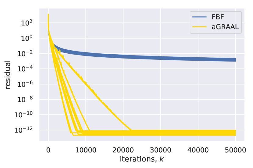
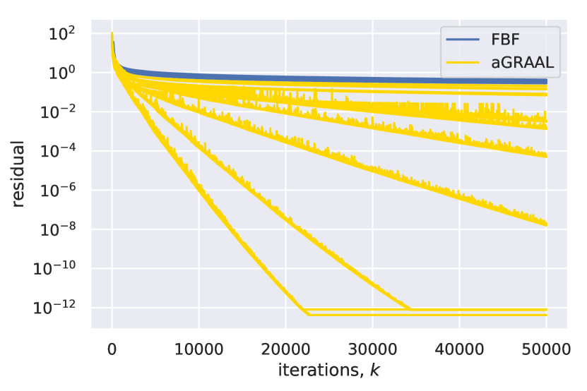
Figure 1: Results for problem (74). Scenario (a) on the left, (b) on the right.

5.2 Convex feasibility problem

Given a number of closed convex sets $C_{i}\subset V$, $i=1,\dots,m$, the convex feasibility problem (CFP) aims to find a point in their intersection: $x\in\cap_{i=1}^{m}C_{i}$. The problem is very general and allows one to represent many practical problems in this form. Projection methods are a standard tool to solve such problem (we refer to [9, 20] for a more in-depth overview). In this note we study a simultaneous projection method: $x^{k+1}=Tx^{k}$, where $T=\frac{1}{m}(P_{C_{1}}+\dots+P_{C_{m}})$. Its main advantage is that it can be easily implemented on a parallel computing architecture. Although it might be slower than the cyclic projection method $x^{k+1}=P_{C_{1}}\dots P_{C_{m}}x^{k}$ in terms of iterations, for large-scale problems it is often much faster in practice due to parallelization and more efficient ways of computing $Tx$.

One can look at the iteration $x^{k+1}=Tx^{k}$ as an application of the Krasnoselskii-Mann scheme for the firmly-nonexpansive operator $T$. By that $(x^{k})$ converges to a fixed point of $T$, which is either a solution of CFP (consistent case) or a solution of the problem $\min_{x}\sum_{i=1}^{m}\operatorname{dist}(x,C_{i})^{2}$ (inconsistent case when the intersection is empty).

To illustrate Remark 3, we show how in many cases aGRAAL with $F=\operatorname{Id}-T$ can accelerate convergence of the simultaneous projection algorithm. We believe, this is quite interesting, especially if one takes into account that our framework works as a black box: it does not require any tuning or a priori information about the initial problem.

Tomography reconstruction. The goal of the tomography reconstruction problem is to obtain a slice image of an object from a set of projections (sinogram). Mathematically speaking, this is an instance of a linear inverse problem

$$Ax=\hat{b},$$ (77)

where $x\in\mathbb{R}^{n}$ is the unknown image, $A\in\mathbb{R}^{m\times n}$ is the projection matrix, and $\hat{b}\in\mathbb{R}^{m}$ is the given sinogram. In practice, however, $\hat{b}$ is contaminated by some noise $\varepsilon\in\mathbb{R}^{m}$, so we observe only $b=\hat{b}+\varepsilon$. It is clear that we can formulate the given problem as CFP with $C_{i}=\{x\colon\langle a_{i},x\rangle=b_{i}\}$. However, since the projection matrix $A$ is often rank-deficient, it is very likely that $b\notin\operatorname{range}(A)$, thus we have to consider the inconsistent case $\min_{x}\sum_{i=1}^{m}\operatorname{dist}(x,C_{i})^{2}$. As the projection onto $C_{i}$ is given by $P_{C_{i}}x=x-\frac{\langle a_{i},x\rangle-b_{i}}{\|a_{i}\|^{2}}a_{i}$, computing $Tx$ reduces to the matrix-vector multiplications which is realized efficiently in most computer processors. Note that our approach only exploits feasibility constraints, which is definitely not a state of the art model for tomography reconstruction. More involved methods would solve this problem with the use of some regularization techniques, but we keep such simple model for illustration purposes only.

As a particular problem, we wish to reconstruct the Shepp-Logan phantom image $256\times 256$ (thus, $x\in\mathbb{R}^{n}$ with $n=2^{16}$) from the far less measurements $m=2^{15}$. We generate the matrix $A\in\mathbb{R}^{m\times n}$ from the scikit-learn library and define $b=Ax+\varepsilon$, where $\varepsilon\in\mathbb{R}^{m}$ is a random vector, whose entries are drawn from $\mathcal{N}(0,1)$. The starting point was chosen as $x^{1}=(0,\dots,0)$ and $\lambda_{0}=1$. In Fig. 2 (left) we report how the residual $\|x^{k}-Tx^{k}\|$ is changing w.r.t. the number of iterations and in Fig. 2 (right) we show the size of steps for aGRAAL scheme. Recall that the CPU time of both is almost the same, so one can reliably state that in this case aGRAAL in fact accelerates the fixed point iteration $x^{k+1}=Tx^{k}$. The information about the steps $\lambda_{k}$ gives us at least some explanation of what we observe: with larger $\lambda_{k}$ the role of $Tx^{k}$ in (3) increases and hence we are faster approaching to the fixed point set.

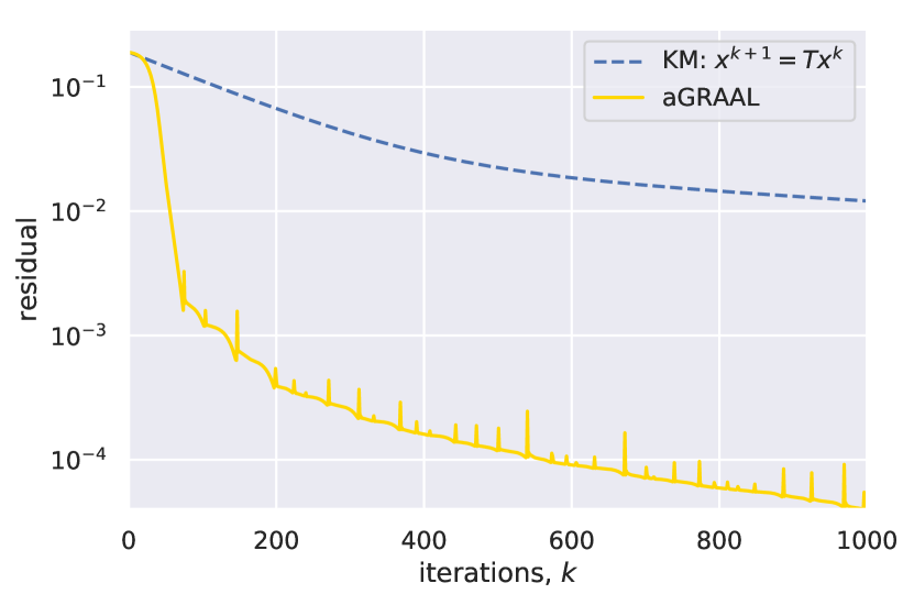
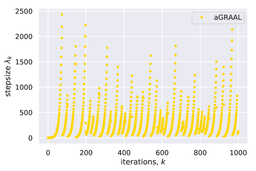
Figure 2: Results for problem (77). Left: the behavior of residual $\|x^{k}-Tx^{k}\|$ for KM and aGRAAL methods. Right: the size of stepsize of $\lambda_{k}$ for aGRAAL

Intersection of balls. Now we consider a synthetic nonlinear feasibility problem. We have to find a point in $x\in\cap_{i=1}^{m}C_{i}$, where $C_{i}=\mathbb{B}(c_{i},r_{i})$, a closed ball with a center $c_{i}\in\mathbb{R}^{n}$ and a radius $r_{i}>0$. The projection onto $C_{i}$ is simple: $P_{C_{i}}x$ equals to $\frac{x-c_{i}}{\|x-c_{i}\|}r_{i}$ if $\|x-c_{i}\|>r_{i}$ and $x$ otherwise. Thus, again computing $Tx=\frac{1}{m}\sum_{i=1}^{m}P_{C_{i}}x$ can be done in parallel very efficiently.

We run two scenarios: with $n=1000$, $m=2000$ and with $n=2000$, $m=1000$. Each coordinate of $c_{i}\in\mathbb{R}^{n}$ is drawn from $\mathcal{N}(0,100)$. Then we set $r_{i}=\|c_{i}\|+1$ that ensures that zero belongs to the intersection of $C_{i}$. The starting point was chosen as the average of all centers: $x^{1}=\frac{1}{m}\sum_{i=1}^{m}c_{i}$. As before, since the cost of iteration of both methods is approximately the same, we show only how the residual $\|Tx^{k}-x^{k}\|$ is changing w.r.t. the number of iterations. To eliminate the role of chance, we plot the results for $100$ random realizations from each of the above scenarios. Fig. 3 depicts the results. As one can see, the difference is again significant.

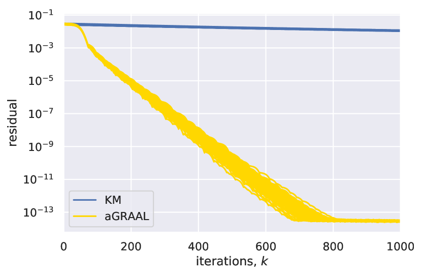
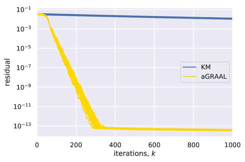
Figure 3: Convergence results for CFP with random balls $C_{i}$. $T=\frac{1}{m}\sum_{i=1}^{m}P_{C_{i}}$. Left: $n=1000$, $m=2000$. Right: $n=2000$, $m=1000$.

5.3 Sparse logistic regression

In this section we demonstrate that even for nice problems as convex composite minimization (5) with Lipschitz $\nabla f$, aGRAAL can be faster than the proximal gradient method or accelerated proximal gradient method. This is interesting, especially since the latter method has a better theoretical convergence rate.

Our problem of interest is a sparse logistic regression

$$\min_{x}J(x):=\sum_{i=1}^{m}\log(1+\exp(-b_{i}\langle a_{i},x\rangle))+\gamma\|x\|_{1},$$ (78)

where $x\in\mathbb{R}^{n}$, $a_{i}\in\mathbb{R}^{n}$, and $b_{i}\in\{-1,1\}$, $\gamma>0$. This is a popular problem in machine learning applications where one aims to find a linear classifier for points $a_{i}$. Let us form a new matrix $K\in\mathbb{R}^{m\times n}$ as $K_{ij}=-b_{i}a_{ij}$ and set $\tilde{f}(y)=\sum_{i=1}^{m}\log(1+\exp(y_{i}))$. Then the objective in (78) is $J(x)=f(x)+g(x)$ with $g(x)=\gamma\|x\|_{1}$ and $f(x)=\tilde{f}(Kx)$. As $\tilde{f}$ is separable, it is easy to derive that $L_{\nabla\tilde{f}}=\frac{1}{4}$. Thus, $L_{\nabla f}=\frac{1}{4}\|K^{T}K\|$.

We compare our method with the proximal gradient method (PGM) and FISTA [11] with a fixed stepsize. We have not included into comparison the extensions of these methods with linesearch, as we are interested in methods that require one evaluation of $\nabla f$ and one of $\operatorname{prox}_{g}$ per iteration. For both methods we set the stepsize as $\lambda=\frac{1}{L_{\nabla f}}=\frac{4}{\|K^{T}K\|}$. We take two popular datasets from LIBSVM [18]: real-sim with $m=72309$, $n=20958$ and kdda-2010 with $m=510302$, $n=2014669$. For both problems we set $\gamma=0.005\|A^{T}b\|_{\infty}$. We are aware of that neither PGM nor FISTA can be considered as the state of the art for (78), stochastic methods seem to be more competitive as the size of the problem is quite large. Overall our motivation is not to propose the best method for (78) but to demonstrate the performance of aGRAAL on some real-world problems.

We run all methods for sufficiently many iterations and compute the energy $J(x^{k})$ in each iteration. If after $k$ iterations the residual was small enough: $\|x^{k}-\operatorname{prox}_{g}(x^{k}-\nabla f(x^{k}))\|\leq 10^{-6}$, we choose the smallest energy value among all methods and set it to $J_{*}$. In Fig. 4 we show how the energy residual $J(x^{k})-J_{*}$ is changing w.r.t. the iterations. Since the dimensions in both problems are quite large, the CPU time for all methods is approximately the same.

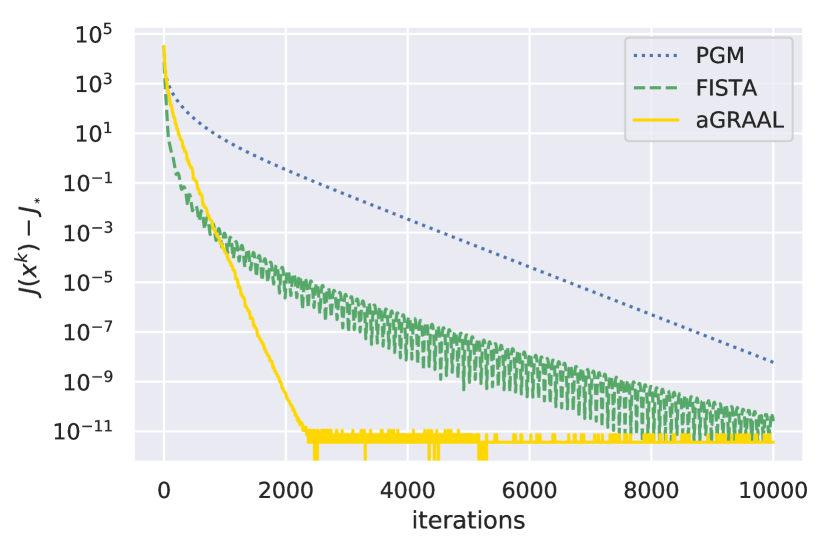
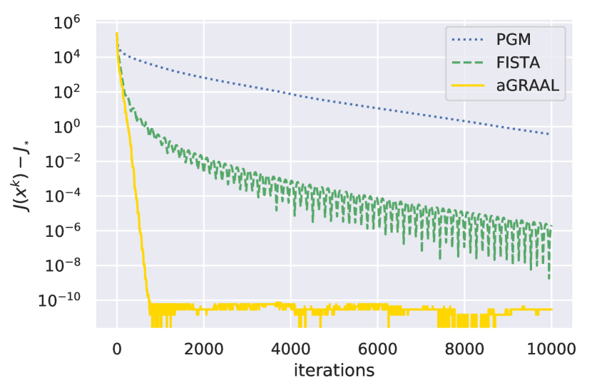
Figure 4: Results for problem (78). Datasets real-sim (left) and kdda-2010 (right).

We have presented the results of only two test problems merely for compactness, in fact similar results were observed for other datasets that we tested: rcv1, a9a, ijcnn1, covtype. An explanation for such a good performance of aGRAAL is of course that for this problem the global Lipschitz constant of $\nabla f$ is too conservative. Notice also that our algorithm did not take into account that in this case $F=\nabla f$ is a potential operator. It would be interesting to see how we can enhance aGRAAL with this information.

5.4 Beyond monotonicity

Finally, we illustrate numerically that aGRAAL can work even for nonmonotone problems.

Nonmonotone equation. We would like to find a non-zero solution of $F(z):=M(z)z=0$, where $M\colon\mathbb{R}^{n}\to\mathbb{R}^{n\times n}$ is a matrix-valued function. This is of course a VI (1) with $g\equiv 0$. We construct $M$ such that $M(z)$ is a symmetric positive semidefinite matrix for any $z$. Thus, $F$ obviously satisfies condition (71), since with $\bar{z}=0$ we have $\langle M(z),z\rangle\geq 0$ for all $z$. This also indicates that $z=0$ is a (trivial) solution of our problem.

For the experiment, we define $M$ as

$$M(z):=t_{1}t_{1}^{T}+t_{2}t_{2}^{T},\quad\text{with}\quad t_{1}=A\sin z,\quad t_{2}=B\exp z,$$ (79)

where $z\in\mathbb{R}^{n}$, $A,B\in\mathbb{R}^{n\times n}$ and the operations $\sin$ and $\exp$ should be understood to apply entrywise. In fact, for our purposes one term $t_{1}t_{1}^{T}$ in $F$ was sufficient, however we want to be sure that a non-zero solution of our problem will not coincide with a solution of a simple problem, like $Az=0$.

For each $n\in\{100,500,1000,5000\}$ we generate $100$ random problems. We run aGRAAL for $10000$ iterations and stopped it whenever the accuracy $\|F(z^{k})\|\leq 10^{-6}$ reached. Table 1 shows the success rate of solving this problem, i.e., we counted only those problems where $\|z^{k}\|$ was large enough to make sure that this is not a trivial solution. We also report the average number of iterations (among all successful instances) the method needs to find a non-trivial solution. The entries of $A$, $B$ are drawn independently from the normal distribution $\mathcal{N}(0,1)$. The starting point is always $z^{1}=(1,\dots,1)$. It is clear that $F$ is not monotone; moreover, the transcendental functions $\sin$, $\exp$ make this problem highly nonlinear.

Table 1: Results of aGRAAL for nonmonotone problem (79)

		$n=100$	$n=500$	$n=1000$	$n=5000$
iter		526	614	667	1532
rate		100	100	100	99

6 Conclusions and further directions

We conclude our work by presenting some possible directions for future research.

Fixed point iteration. It is interesting to represent scheme (10) as a fixed point iteration. To this end, let

$$G=\begin{bmatrix}\operatorname{Id}&0\\ 0&\operatorname{prox}_{\lambda g}\end{bmatrix}\qquad R=\begin{bmatrix}\frac{1}{\varphi}\operatorname{Id}&\frac{\varphi-1}{\varphi}\operatorname{Id}\\ \frac{1}{\varphi}\operatorname{Id}&\qquad\frac{\varphi-1}{\varphi}\operatorname{Id}-\lambda F\end{bmatrix}.$$ (80)

Then it is not difficult to see that we can rewrite (10) as

$$\binom{\bar{z}^{k}}{z^{k+1}}=(G\circ R)\binom{\bar{z}^{k-1}}{z^{k}}.$$ (81)

If we now set $\mathbf{u}^{k}=(\bar{z}^{k-1},z^{k})$, the above equation simplifies to $\mathbf{u}^{k+1}=GR\mathbf{u}^{k}$. However, so far it not clear how to derive convergence of (10) from the fixed point perspective. Although, $G$ is a firmly-nonexpansive operator, $R$ is definitely not; thus, it is difficult to say something meaningful about $G\circ R$.

Inertial extensions. Starting from the paper [47], it is observed that using some inertia for the optimization algorithm often accelerates the latter. Later, papers [1, 40, 32, 14] extend this idea to a more general case with monotone operators. In our case it will be in particular interesting to do so, since our scheme

$$z^{k+1}=\operatorname{prox}_{\lambda g}(\bar{z}^{k}-\lambda F(z^{k}))$$ (82)

uses $\bar{z}^{k}$ as a convex combination of all previous iterates $z^{1}\dots,z^{k}$. This is completely opposite to the inertial methods, where one uses $z^{k}+\alpha(z^{k}-z^{k-1})$ for some $\alpha>0$.

Bregman distance. For many VI methods it is possible to derive their analogues for the Bregman distances, as this is done for the the extragradient method [31] by extensions  [43, 45]. It is possible to do so for GRAAL? This extension is not trivial since, for example, in (2) we have used the identity (7), where the linear structure was explicitly used.

Stochastic settings. For large-scale problems it is often the case that even computing $F(z^{k})$ becomes prohibitively expensive. For this reason, the stochastic VI methods that compute $F(z^{k})$ approximately can be advantageous over their deterministic counterparts, as it was shown in [6, 27]. It is interesting to derive similar extensions for GRAAL. The same concerns the coordinate extensions of GRAAL.

Continuous dynamic. Many discrete optimization/VI methods can be studied from the continuous perspective which may shed light on the discrete method. Originated from 60-s, this line of research was popularized by many authors, see [2, 5, 4, 7] and references therein. This research brings new and often deeper understanding of the respective iterative schemes, as, for instance, the case with the Nesterov acceleration in [53, 4]. For aGRAAL it is a challenging task to derive a continuous scheme, since the function $\lambda(t)$ cannot be defined in advance.

Acknowledgements.

Y. Maltsky was supported by German Research Foundation grant SFB755-A4. The author would like to thank Anna–Lena Martins, Panayotis Mertikopoulos, Matthew Tam, associate editor and anonymous referees for their useful comments that have significantly improved the quality of the paper.

References

- [1] Alvarez, F., and Attouch, H. An inertial proximal method for maximal monotone operators via discretization of a nonlinear oscillator with damping. Set-Valued Analysis 9, 1-2 (2001), 3–11.
- [2] Antipin, A. S. Minimization of convex functions on convex sets by means of differential equations. Differential equations 30, 9 (1994), 1365–1375.
- [3] Arrow, K. J., Hurwicz, L., and Uzawa, H. Studies in linear and non-linear programming. Stanford University Press, 1958.
- [4] Attouch, H., Chbani, Z., Peypouquet, J., and Redont, P. Fast convergence of inertial dynamics and algorithms with asymptotic vanishing viscosity. Mathematical Programming 168, 1-2 (2018), 123–175.
- [5] Attouch, H., and Cominetti, R. A dynamical approach to convex minimization coupling approximation with the steepest descent method. Journal of Differential Equations 128, 2 (1996), 519–540.
- [6] Baes, M., Bürgisser, M., and Nemirovski, A. A randomized mirror-prox method for solving structured large-scale matrix saddle-point problems. SIAM Journal on Optimization 23, 2 (2013), 934–962.
- [7] Banert, S., and Boţ, R. I. A forward-backward-forward differential equation and its asymptotic properties. Journal of Convex Analysis 25, 2 (2018), 371–388.
- [8] Bauschke, H. H., Bolte, J., and Teboulle, M. A descent lemma beyond lipschitz gradient continuity: first-order methods revisited and applications. Mathematics of Operations Research 42, 2 (2016), 330–348.
- [9] Bauschke, H. H., and Borwein, J. M. On projection algorithms for solving convex feasibility problems. SIAM Review 38, 3 (1996), 367–426.
- [10] Bauschke, H. H., and Combettes, P. L. Convex Analysis and Monotone Operator Theory in Hilbert Spaces. Springer, New York, 2011.
- [11] Beck, A., and Teboulle, M. A fast iterative shrinkage-thresholding algorithm for linear inverse problem. SIAM Journal on Imaging Sciences 2, 1 (2009), 183–202.
- [12] Bello Cruz, J., and Díaz Millán, R. A variant of forward-backward splitting method for the sum of two monotone operators with a new search strategy. Optimization 64, 7 (2015), 1471–1486.
- [13] Berinde, V. Iterative approximation of fixed points, vol. 1912. Springer, 2007.
- [14] Boţ, R. I., and Csetnek, E. R. An inertial forward-backward-forward primal-dual splitting algorithm for solving monotone inclusion problems. Numerical Algorithms 71, 3 (2016), 519–540.
- [15] Censor, Y., Gibali, A., and Reich, S. The subgradient extragradient method for solving variational inequalities in Hilbert space. Journal of Optitmization Theory and Applications 148 (2011), 318–335.
- [16] Chambolle, A., and Pock, T. A first-order primal-dual algorithm for convex problems with applications to imaging. Journal of Mathematical Imaging and Vision 40, 1 (2011), 120–145.
- [17] Chambolle, A., and Pock, T. On the ergodic convergence rates of a first-order primal–dual algorithm. Mathematical Programming 159, 1-2 (2016), 253–287.
- [18] Chang, C.-C., and Lin, C.-J. LIBSVM: a library for support vector machines. ACM transactions on intelligent systems and technology (TIST) 2, 3 (2011), 27.
- [19] Chen, G. H., and Rockafellar, R. T. Convergence rates in forward–backward splitting. SIAM Journal on Optimization 7, 2 (1997), 421–444.
- [20] Combettes, P. The convex feasibility problem in image recovery. Advances in imaging and electron physics 95 (1996), 155–270.
- [21] Facchinei, F., and Pang, J.-S. Finite-Dimensional Variational Inequalities and Complementarity Problems, Volume I and Volume II. Springer-Verlag, New York, USA, 2003.
- [22] Giselsson, P., Fält, M., and Boyd, S. Line search for averaged operator iteration. In Decision and Control (CDC), 2016 IEEE 55th Conference on (2016), IEEE, pp. 1015–1022.
- [23] Harker, P. T. A variational inequality approach for the determination of oligopolistic market equilibrium. Mathematical Programming 30, 1 (1984), 105–111.
- [24] He, B. A new method for a class of linear variational inequalities. Mathematical Programming 66, 1-3 (1994), 137–144.
- [25] Ishikawa, S. Fixed points by a new iteration method. Proceedings of the American Mathematical Society 44, 1 (1974), 147–150.
- [26] Iusem, A. N., and Svaiter, B. F. A variant of Korpelevich’s method for variational inequalities with a new search strategy. Optimization 42 (1997), 309–321.
- [27] Juditsky, A., Nemirovski, A., and Tauvel, C. Solving variational inequalities with stochastic mirror-prox algorithm. Stochastic Systems 1, 1 (2011), 17–58.
- [28] Khobotov, E. N. Modification of the extragradient method for solving variational inequalities and certain optimization problems. USSR Computational Mathematics and Mathematical Physics 27 (1989), 120–127.
- [29] Kinderlehrer, D., and Stampacchia, G. An introduction to variational inequalities and their applications, vol. 31. SIAM, 1980.
- [30] Konnov, I. A class of combined iterative methods for solving variational inequalities. Journal of Optimization Theory and Applications 94, 3 (1997), 677–693.
- [31] Korpelevich, G. M. The extragradient method for finding saddle points and other problems. Ekonomika i Matematicheskie Metody 12, 4 (1976), 747–756.
- [32] Lorenz, D., and Pock, T. An inertial forward-backward algorithm for monotone inclusions. Journal of Mathematical Imaging and Vision 51, 2 (2015), 311–325.
- [33] Lu, H., Freund, R. M., and Nesterov, Y. Relatively smooth convex optimization by first-order methods, and applications. SIAM Journal on Optimization 28, 1 (2018), 333–354.
- [34] Luke, R. D., Thao, N. H., and Tam, M. K. Quantitative convergence analysis of iterated expansive, set-valued mappings. Mathematics of Operations Research (2018).
- [35] Lyashko, S. I., Semenov, V. V., and Voitova, T. A. Low-cost modification of Korpelevich’s method for monotone equilibrium problems. Cybernetics and Systems Analysis 47 (2011), 631–639.
- [36] Malitsky, Y. Reflected projected gradient method for solving monotone variational inequalities. SIAM Journal on Optimization 25, 1 (2015), 502–520.
- [37] Malitsky, Y. Proximal extrapolated gradient methods for variational inequalities. Optimization Methods and Software 33, 1 (2018), 140–164.
- [38] Malitsky, Y. V., and Semenov, V. V. An extragradient algorithm for monotone variational inequalities. Cybernetics and Systems Analysis 50, 2 (2014), 271–277.
- [39] Monteiro, R. D., and Svaiter, B. F. Complexity of variants of Tseng’s modified FB splitting and Korpelevich’s methods for hemivariational inequalities with applications to saddle-point and convex optimization problems. SIAM Journal on Optimization 21, 4 (2011), 1688–1720.
- [40] Moudafi, A., and Oliny, M. Convergence of a splitting inertial proximal method for monotone operators. Journal of Computational and Applied Mathematics 155, 2 (2003), 447–454.
- [41] Murphy, F. H., Sherali, H. D., and Soyster, A. L. A mathematical programming approach for determining oligopolistic market equilibrium. Mathematical Programming 24, 1 (1982), 92–106.
- [42] Naimpally, S., and Singh, K. Extensions of some fixed point theorems of rhoades. Journal of mathematical analysis and applications 96, 2 (1983), 437–446.
- [43] Nemirovski, A. Prox-method with rate of convergence for variational inequalities with lipschitz continuous monotone operators and smooth convex-concave saddle point problems. SIAM Journal on Optimization 15, 1 (2004), 229–251.
- [44] Nemirovsky, A. Information-based complexity of linear operator equations. Journal of Complexity 8, 2 (1992), 153–175.
- [45] Nesterov, Y. Dual extrapolation and its applications to solving variational inequalities and related problems. Mathematical Programming 109, 2-3 (2007), 319–344.
- [46] Pang, J.-S. Error bounds in mathematical programming. Mathematical Programming 79, 1-3 (1997), 299–332.
- [47] Polyak, B. Some methods of speeding up the convergence of iteration methods. U.S.S.R. Computational Mathematics and Mathematical Physics 4, 5 (1967), 1–17.
- [48] Popov, L. D. A modification of the Arrow-Hurwicz method for finding saddle points. Mathematical Notes 28, 5 (1980), 845–848.
- [49] Qihou, L. On Naimpally and Singh’s open questions. Journal of mathematical analysis and applications 124, 1 (1987), 157–164.
- [50] Solodov, M. V. Convergence rate analysis of iteractive algorithms for solving variational inequality problems. Mathematical Programming 96, 3 (2003), 513–528.
- [51] Solodov, M. V., and Svaiter, B. F. A new projection method for variational inequality problems. SIAM Journal on Control and Optimization 37, 3 (1999), 765–776.
- [52] Solodov, M. V., and Tseng, P. Modified projection-type methods for monotone variational inequalities. SIAM Journal on Control and Optimization 34, 5 (1996), 1814–1830.
- [53] Su, W., Boyd, S., and Candes, E. A differential equation for modeling Nesterov’s accelerated gradient method: Theory and insights. In Advances in Neural Information Processing Systems (2014), pp. 2510–2518.
- [54] Themelis, A., and Patrinos, P. Supermann: a superlinearly convergent algorithm for finding fixed points of nonexpansive operators. IEEE Transactions on Automatic Control (2019).
- [55] Tran-Dinh, Q., Kyrillidis, A., and Cevher, V. Composite self-concordant minimization. The Journal of Machine Learning Research 16, 1 (2015), 371–416.
- [56] Tseng, P. On linear convergence of iterative methods for the variational inequality problem. Journal of Computational and Applied Mathematics 60, 1-2 (1995), 237–252.
- [57] Tseng, P. A modified forward-backward splitting method for maximal monotone mappings. SIAM Journal on Control and Optimization 38 (2000), 431–446.
- [58] Yang, J., and Liu, H. A modified projected gradient method for monotone variational inequalities. Journal of Optimization Theory and Applications 179, 1 (2018), 197–211.