An accurate mass determination for Kepler-1655b, a moderately-irradiated world with a significant volatile envelope

Abstract

We present the confirmation of a small, moderately-irradiated ($F=155\pm 7$ F_⊕) Neptune with a substantial gas envelope in a $P$=11.8728787$\pm$0.0000085-day orbit about a quiet, Sun-like G0V star Kepler-1655. Based on our analysis of the Kepler light curve, we determined Kepler-1655b’s radius to be 2.213$\pm$0.082 R_⊕. We acquired 95 high-resolution spectra with TNG/HARPS-N, enabling us to characterize the host star and determine an accurate mass for Kepler-1655b  of 5.0$\pm^{3.1}_{2.8}$  M_⊕  via Gaussian-process regression. Our mass determination excludes an Earth-like composition with 98% confidence. Kepler-1655b falls on the upper edge of the evaporation valley, in the relatively sparsely occupied transition region between rocky and gas-rich planets. It is therefore part of a population of planets that we should actively seek to characterize further.

1. Introduction

In our own solar system, we see a sharp transition between the inner planets, which are small ($R_{p}\leq$ 1 R_⊕) and rocky, and the outer planets that are larger ($R_{p}\geq 3.88$ R_⊕), much more massive, and have thick, gaseous envelopes. For exoplanets with radii intermediate to that of the Earth (1 R_⊕) and Neptune (3.88 R_⊕), several factors go into determining whether planets acquire or retain a thick gaseous envelope. Several studies have determined statistically from radius and mass determinations of exoplanets that most planets smaller than 1.6 R_⊕ are rocky, i.e. they do not have large envelopes but only a thin, secondary atmosphere, if any at all (Rogers, 2015; Weiss & Marcy, 2014; Dressing & Charbonneau, 2015; Lopez & Rice, 2016; Lopez, 2016; Lopez & Fortney, 2014; Buchhave et al., 2016; Gettel et al., 2016). Others have found that planets in less irradiated orbits tend to be more likely to have gaseous envelopes than more highly irradiated planets (Hadden & Lithwick, 2014; Jontof-Hutter et al., 2016). However, it is still unclear under which circumstances a planet will obtain and retain a thick gaseous envelope and how this is related to other parameters, such as stellar irradiation levels.

The characterization of the mass of a small planet in an orbit of a few days to a few months around a Sun-like star (i.e. in the incident flux range $\approx$ 1-5000 F_⊕) is primarily limited by the stellar magnetic features acting over this timescale and producing RV variations that compromise our mass determinations. Magnetic fields produce large, dark starspots and bright faculae on the stellar photosphere. These features induce RV variations modulated by the rotation of the star and varying in amplitude as the features emerge, grow and decay. There are two physical processes at play: (i) dark starspots and bright faculae break the Doppler balance between the approaching blueshifted stellar hemisphere and the receding redshifted half of the star (Saar & Donahue, 1997; Lagrange et al., 2010; Boisse et al., 2012; Haywood et al., 2016); (ii) they inhibit the star’s convective motions, and this suppresses part of the blueshift that naturally arises from convection (Dravins et al., 1981; Meunier et al., 2010a, b; Dumusque et al., 2014; Haywood et al., 2016).

In this paper we report the confirmation of Kepler-1655b, a mini Neptune orbiting a Sun-like star, first noted as a planet candidate (KOI-280.01) by Borucki et al. (2011). Kepler-1655b  straddles the valley between the small, rocky worlds and the larger, gas-rich worlds. It is also in a moderately-irradiated orbit. We present the $Kepler$ and HARPS-N observations for this system in Section 2. Based on these datasets, we determine the properties of the host star (Section 3), statistically validate Kepler-1655b as a planet (Section 4), measure Kepler-1655b’s radius (Section 5) and mass (Section 6). Using these newly-determined stellar and planetary parameters, we place Kepler-1655b among other exoplanets found to date and investigate the influence of incident flux on planets with thick gaseous envelopes, as compared with gas-poor, rocky planets (Section 7).

2. Observations

2.1. Kepler Photometry

Kepler-1655 was monitored with Kepler in 29.4 min, long-cadence mode between quarters Q0 and Q17, and in 58.9 sec, short-cadence mode in quarters Q2-Q3 and Q6-Q17, covering a total time period of 1,459.49 days (BJD 2454964.51289 – 2456424.00183).

The simple aperture flux (SAP) shows large long-term variations on the timescale of a Kepler quarter due to differential velocity aberration, which without adequate removal obscures astrophysical stellar rotation signals as small as those expected for Kepler-1655. The Presearch Data Conditioning (PDC) reduction from Data Release 25 (DR25) did not remove these long-term trends completely due to an inadequate choice of aperture pixels. The PDC reduction from DR21, however, had a particular choice of apertures which was much more effective at removing these trends. We therefore worked with the PDCSAP light curve from Data Release 21 (Stumpe et al., 2014; Smith et al., 2012; Stumpe et al., 2012) to estimate the stellar and planet parameters.

We compared the PDC (DR21) light curve with the principle component analysis (PCA) light curve and the Data Validation (DV) light curve, generated as described in Coughlin & López-Morales (2012); see also López-Morales et al. (2016) for a detailed description of these two types of analyses. All three lightcurves are plotted in Figure 1. The PDCSAP (DR 21) and PCA light curves show very similar features. They both display little variability aside from the transits of Kepler-1655b, which indicates that Kepler-1655  is a quiet, low-activity star. Some larger dispersion is visible in quarters Q0-Q2, which is likely to be the signature of rotation-modulated activity (more on this in Section 6.2). We note that Q12 has increased systematics in all three detrendings, possibly due to the presence of three coronal mass ejections which affected spacecraft and detector performance throughout the quarter (Van Cleve et al., 2016). The DV detrending also shows increased systematics, most likely due to the harmonic removal module in DV, which operates on a per-quarter basis (Li et al., 2017).

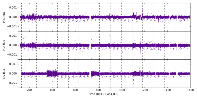
Figure 1.— Full Q0–Q17 long cadence Kepler lightcurve detrended using: Top – Presearch Data Conditioning Simple Aperture Photometry (PDCSAP, DR21); Middle – Principal Component Analysis (PCA); Bottom – Data Validation (DV). The dashed lines mark the start of each Kepler quarter.

2.2. HARPS-N Spectroscopy

We observed Kepler-1655 with the HARPS-N instrument (Cosentino et al., 2012) on the Telescopio Nazionale Galileo (TNG) at La Palma, Spain over two seasons between 2015 June 7 and 2016 November 13. The spectra were processed using the HARPS Data Reduction System (DRS)(Baranne et al., 1996). The cross-correlation was performed using a G2 spectral mask (Pepe et al., 2002). The RV measurements and the spectroscopic activity indicators are provided in Table 4. The median, minimum and maximum signal to noise ratio of the HARPS spectra at the centre of the spectral order number 50 are 51.8, 24.8 and 79.2, respectively.

The host star is fainter than typical RV targets and its RVs can be potentially affected by moonlight contamination. We followed the procedure detailed in Malavolta et al. (2017b) and determined that none of our measurements were affected, including those carried out near full Moon. In all cases the RV of the star with respect to the observer rest frame, i.e. the difference between the systemic RV of the star and the barycentric RV correction, was higher than -25 km.s^-1, that is around three times the FWHM of the CCF, thus avoiding any moonlight contamination.

3. Stellar properties of Kepler-1655

Kepler-1655 is a G0V star with an apparent V magnitude of $11.05\pm 0.08$, located at a distance of $230.41\pm 28.14$ pc from the Sun, according to the Gaia data release DR1 (Gaia Collaboration et al., 2016). All relevant stellar parameters can be found in Table 3.

We added all individual HARPS-N spectra together and performed a spectroscopic line analysis. Equivalent widths of a list of iron lines (Fe I and Fe II) (Sousa et al., 2011) were automatically determined using ARESv2 (Sousa et al., 2015). We then used them, along with a grid of ATLAS plane-parallel model atmospheres (Kurucz, 1993), to determine the atmospheric parameters, assuming local thermodynamic equilibrium in the 2014 version of the MOOG code (Sneden et al., 2012). We used the iron abundance as a proxy for the metallicity. More details on the method are found in Sousa (2014) and references therein. We corrected the surface gravity resulting from this analysis to a more accurate value following Mortier et al. (2014).

We quadratically added systematic errors to our precision errors, intrinsic to our spectroscopic method. For the effective temperature we added a systematic error of $60$ K, for the surface gravity $0.1$ dex, and for metallicity $0.04$ dex (Sousa et al., 2011).

We found an effective temperature of 6148 K and a metallicity of -0.24. These values are consistent with the values reported by Huber et al. (2013) (6134 K and -0.24, respectively), based on a spectral synthesis analysis of a TRES spectrum.

As a sanity check we also estimated the temperature and metallicity from the HARPS-N CCFs according to the method of Malavolta et al. (2017a) and obtained a similar result (6151 $\pm 34$ K, $-0.27\pm 0.03$, internal errors only).

The stellar mass and radius were derived using a Bayesian estimation (da Silva et al., 2006) and a set of PARSEC isochrones (Bressan et al., 2012). We used the effective temperature and metallicity from the spectroscopic analysis as input. We ran the analysis twice, once using the apparent V magnitude and parallax and once using the asteroseismic values $\Delta\nu$ and $\nu_{max}$ obtained by Huber et al. (2013). The values are consistent, with the ones resulting from the asteroseismology being more precise. We use the latter throughout the rest of the paper (see Table 3). These mass and radius values are also consistent with the ones obtained by Huber et al. (2013) and Silva Aguirre et al. (2015). The resulting stellar density is consistent with what is found by analysing the transit shape (see Section 5). This analysis also determined an age of $2.56\pm 1.06$ Gyr, consistent with the $3.27\pm^{0.59}_{0.64}$ Gyr from the analysis of Silva Aguirre et al. (2015).

The spectral synthesis used by Huber et al. (2013) revealed a $v\,\sin{i_{\rm star}}$ of $3.5\pm 0.5$$\rm km\,s^{-1}$, making Kepler-1655 a relatively slowly rotating star. In an asteroseismology analysis, Campante et al. (2015) determined the stellar inclination to be between 38.4 and 90 degrees (within the 95.4% highest posterior density credible region). This value translates into an upper limit for the rotation period of $14.8\pm 2.4$ days, and a lower limit of $9.2\pm 2.4$ days which are consistent with the rotation period we determine from the Kepler light curve (see Section 6.2).

4. Statistical Validation

The detection of a spectroscopic orbit in phase with the photometric ephemeris through RV observations is the gold standard for proving that transit signals found in Kepler data are genuine exoplanets. In the case of Kepler-1655b, however, we do not detect the planet’s reflex motion at high significance through our HARPS-N RV observations (see Section 6). Instead, in this section, we show that the transit signal is very likely a genuine exoplanet by calculating the astrophysical false positive probabilities using the open source tool vespa (Morton, 2012, 2015), and by interpreting additional observations that are not considered by the vespa software.

Assessement of false positive probabilities using Vespa

Vespa calculates the likelihood that a transit signal is caused by a planet compared to the likelihood that the transit signal is caused by some other astrophysical phenomenon such as an eclipsing binary, either on the foreground star, or on another star in the photometric aperture. Vespa compares the shape of the observed transit to what would be expected for these different scenarios, and imposes priors based on the density of stars in the field, constraints on other stars in the aperture from high resolution imaging, limits on putative secondary eclipses, and differences in the depths of odd and even eclipses (to constrain scenarios where the signal is caused by an eclipsing binary with double the orbital period we find). We include as constraints two adaptive optics images acquired with the Palomar PHARO-AO system in J and K bands, downloaded from the Kepler Community Follow-Up Program (CFOP) webpage. In the case of Kepler-1655, we also impose the constraint that we definitively rule out scenarios where Kepler-1655b is actually an eclipsing binary based on our HARPS-N RV observations, because we have a strong upper limit on the mass measurement requiring that any companion in a short period orbit be planetary.

Given these constraints, we find a false positive probability of $2\times 10^{-3}$ for Kepler-1655b, which is considerably lower than the $10^{-2}$ threshold commonly used to validate Kepler candidates (Rowe et al., 2014; Morton et al., 2016). The dominant false positive scenario

is that the Kepler-1655 system is a hierarchical eclipsing binary, where a physically associated low-mass eclipsing binary system near to Kepler-1655 is causing the transit signal.

Additional observational constraints

We see no evidence for the existence of a companion star to Kepler-1655  according to AO imaging (see previous paragraph). The maximum peak-to-peak RV variation observed by HARPS-N is well below 20 m.s^-1(see Section 6). These two observational constraints entirely rule out a foreground eclipsing binary scenario. This drops the false positive probability by about a factor of 10 from the vespa estimate and thus places the false positive probability well below the threshold of 1% that is typically used.

The Kepler short cadence data, which did not go into the original vespa analysis, puts further constraints on these scenarios. The dominant scenario that arises from the vespa calculations is the hierarchical scenario. We show that this is entirely ruled out by our short cadence data. With the short cadence photometry, we resolve transit ingress and egress, measuring the duration of ingress/egress, $t_{1,2}$, to be 10 $\pm$ 3 minutes, with ingress and egress each taking up 7% $\pm$ 2% of the total mid-ingress to mid-egress transit duration, $t_{1.5,3.5}$. The ratio between the transit ingress/egress time and the duration, $f=t_{1,2}/t_{1.5,3.5}$, is a measurement of the largest possible companion to star radius ratio, independent of the amount of blending in the light curve. If we assume that the transit is caused by a background object, the faintest background object that could cause the signal we see is only a factor of $f^{2}/(R_{p}/R_{\star})^{2}$ = 12 $\pm$ 6 times fainter than Kepler-1655. For a physically-associated star, this brightness difference corresponds to roughly a late K-dwarf, with stellar radius of about 0.7 R_⊙. The largest physically-associated object which could cause the transit shape we see is therefore about $R_{\rm companion}\simeq$0.7 R_⊙$\times f\simeq 6$ R_⊕, and therefore of planetary size.

The last plausible scenario that remains is that of a hierarchical planet. Even though we cannot rule it out, it is a very unlikely scenario. The stringent limits on false positive scenarios from our vespa analysis, the lack of evidence for a companion star, the fact that small planets are considerably more common than large planets, and the fact that we have a tentative detection of the spectroscopic orbit of Kepler-1655b all give us the highest confidence that Kepler-1655b is in fact a genuine planet transiting Kepler-1655.

5. Radius of Kepler-1655b from transit analysis

We fit the PDCSAP short cadence light curves produced by the Kepler pipeline of Kepler-1655. We flatten the light curve by fitting second order polynomials

to the out-of-transit light curves near transits, and dividing the best-fit polynomial from the light curve. The PDCSAP short cadence light curves have had some systematics removed, but there are still a considerable number of discrepant data points in the light curve, especially towards the end of the original Kepler mission, when the second of four reaction wheels was close to failure. We exclude outliers from the phase-folded light curve by dividing it into bins of a few minutes. Within each of these bins, we then exclude 3-sigma outliers, although we find that a more conservative 5-sigma clipping does not change the resulting planet parameters significantly.

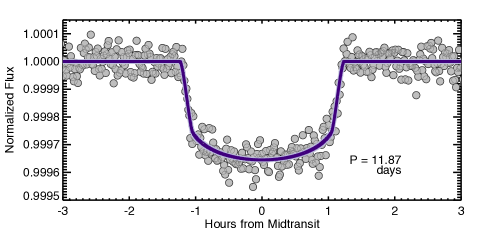
Figure 2.— Short-cadence Kepler transit light curve of Kepler-1655b. Gray dots are the short cadence data binned in roughly 30-second intervals. The line is the maximum-likelihood transit model.

We then fit the transit light curve with a transit model (Mandel & Agol, 2002) using a Markov Chain Monte Carlo (MCMC) algorithm with an affine invariant sampler (Goodman & Weare, 2010). We account for the 58.34-second short-cadence integration time by oversampling model light curves by a factor of 10 and performing a trapezoidal integration. We fit for the planetary orbital period, transit time, scaled semi-major axis ($a/R_{\star}$), the planetary to stellar radius ratio ($R_{p}/R_{\star}$), the orbital inclination, and quadratic limb darkening parameters $q_{1}$ and $q_{2}$, as defined by Kipping (2013). We impose Gaussian priors on the traditional limb darkening parameters $u_{1}$ and $u_{2}$, centered at the values predicted by Claret & Bloemen (2011), with widths of 0.07 in each parameter (which is the typical systematic uncertainty in model limb darkening parameters found by Müller et al. 2013). We sample the parameter space using an ensemble of 50 walkers, evolved for 20,000 steps. We confirm that the MCMC chains were well mixed by calculating the Gelman-Rubin convergence statistics (Gelman & Rubin, 1992).

A binned short-cadence transit light curve and the best-fit model is shown in Figure 2.

The ultra-precise Kepler short cadence data resolves the transit ingress and egress for Kepler-1655b, and therefore is able to precisely measure the planetary impact parameter. We find that Kepler-1655b transits near the limb of its host star, with an impact parameter of 0.85 ${}^{+.03}_{-.07}$, which makes the radius ratio somewhat larger than would likely be inferred from a fit to the long-cadence data alone (without a prior placed on the stellar density and eccentricity).

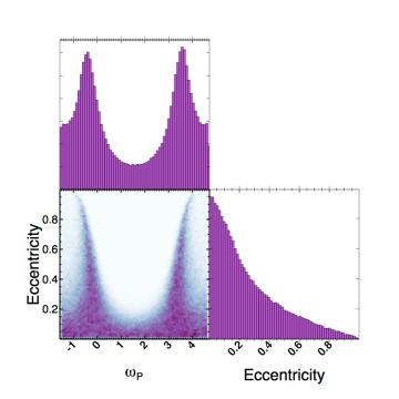
Figure 3.— Correlation plots between the orbital eccentricity of Kepler-1655b and its argument of periastron. Marginalized histograms of these parameters are shown alongside the correlation plot.

As a sanity check, we also fit the transits of Kepler-1655b using the Data Validation (DV) long-cadence light curve (not including quarters Q4, Q8 and Q12) using EXOFAST-1 (Eastman et al., 2013).

All parameter estimates fitted via this method are consistent with the results we obtained from our short-cadence analysis, including the eccentricity.

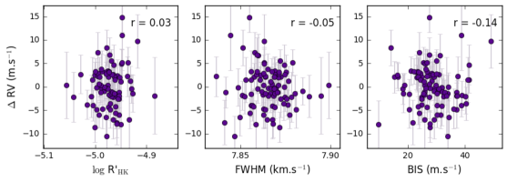
Figure 4.— Plots of the HARPS RV variations vs. the $\log R^{\prime}_{\rm HK}$ index, the FWHM and the BIS of the cross-correlation function. The Spearman correlation coefficients for each pair of variables are given in the top right hand corner of each panel. We find no significant correlations.

5.1. Constraint on the eccentricity via asterodensity profiling

We placed constraints on the eccentricity, $e$, and argument of periastron, $\omega_{p}$, of Kepler-1655b’s orbit by comparing our measured scaled semimajor axis ($a/R_{\star}$) from our short-cadence transit fits (see Section 5) and the precisely-known asteroseismic stellar parameters (listed in Table 3). We followed the procedure outlined by Dawson & Johnson (2012) in their Section 3.4 and explored parameter space using an MCMC analysis with affine invariant ensemble sampling (Goodman & Weare, 2010). We find that Kepler-1655b’s orbit is consistent with circular, although some solutions with high eccentricity and finely tuned arguments of periastron are allowed. Our analysis gives 68% and 95% confidence upper limits of $e_{68\%}<0.31$ and $e_{95\%}<0.71$, respectively. The two-dimensional probability distribution of allowed $e$ and $\omega_{p}$ is shown in Figure 3. These distributions and upper limits are fully consistent with those obtained in our RV analysis (see Table 3 and Figure 14).

6. Mass of Kepler-1655b from RV analysis

The main obstacle to determining robust planet masses arises from the intrinsic magnetic activity of the host star.

Kepler-1655 does not present particularly high levels of magnetic activity. In fact, the magnetic behavior exhibited in its light curve, spectroscopic activity indicators and RV curve is very similar to that of the Sun during its low-activity, “quiet” phase. However, ongoing observations of the Sun as a star show activity-induced RV variations with an RMS of 1.6 m.s^-1 even though it is now entering the low phase of its 11-year magnetic activity cycle (Dumusque et al., 2015). More generally, several large spectroscopic surveys have shown that even the quietest stars display activity-driven RV variations of order 1-2 m.s^-1 (eg. the California Planet Search (Isaacson & Fischer, 2010); the HARPS-N Rocky Planet Search (Motalebi et al., 2015)).

In the current era of confirming and characterizing planets with reflex motions of 1-2 m.s^-1, accounting for the effects of magnetically-induced RV noise/signals, even in stars deemed to be “quiet”, becomes a necessary precaution. This is the only way we will determine planetary masses accurately and reliably (let alone precisely).

In the case of Kepler-1655, we estimate that the rotationally-modulated, activity-induced RV variations have an RMS of order 0.5 m.s^-1. Furthermore, the stellar rotation and planetary orbital periods are very close to each other, at 13 and 11 days, respectively. We perform an RV analysis based on Gaussian process (GP) regression, which can account for low-amplitude, quasi-periodic RV variations modulated by the star’s rotation.

6.1. Preliminary investigations

Firstly, we perform some basic checks on the spectroscopic data available to us. We investigate whether the spectroscopically-derived activity indicators are reliable, and whether they provide any useful information for our analysis. Secondly, we determine the stellar rotation period and active-region evolution timescale from the PDCSAP lightcurve. Thirdly, we look at the sampling strategy of the observations. In particular, we compare the two stellar timescales (rotation and evolution) to the orbital period of Kepler-1655b and investigate how well all three timescales are sampled.

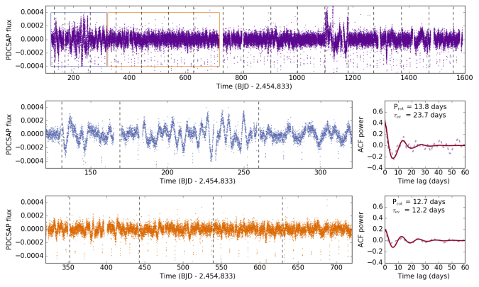
Figure 5.— Autocorrelation function (ACF) analysis. Top panel: full PDCSAP light curve, including transits of Kepler-1655b. Middle panels: zoom-in on a 200-day stretch of light curve during which the star is active, and corresponding ACF (dashed line), overlaid with our MCMC fit (solid line). Bottom panels: zoom-in on a quiet 400-day stretch of the light curve, with corresponding ACF. Note that the transits were excluded for the computation of the ACFs. The dashed lines mark the start of each Kepler quarter.

6.1.1 “Traditional” spectroscopic activity indicators

The average value of the $\log R^{\prime}_{\rm HK}$ index (-4.97) is close to that of the Sun in its low-activity phase ($\approx-5.0$), implying that Kepler-1655 is a relatively quiet star.

Figure 4 shows the RV observations plotted against the “traditional” spectroscopic activity indicators: the $\log R^{\prime}_{\rm HK}$ index, computed from the DRS pipeline, which is a measure of the emission present in the core of the Ca ii H & K lines; the full width at half maximum (FWHM) and bisector span (BIS) of the cross-correlation function, which tell us about the asymmetry of the cross-correlation function (Queloz et al., 2001). We see no significant correlations between the RVs and any of these activity indicators. This is expected as they are measurements that have been averaged over the whole stellar disc and small-scale structures such as spots and faculae, if present, are therefore likely to blur out. Moreover, the cross-correlation function is made up of many thousands of spectral lines whose shapes are all affected by stellar activity in different ways (depending on factors such as their formation depth, Landé factor, excitation potential, etc.).

Reliability of the $\log R^{\prime}_{\rm HK}$ index for this star

A recent study by Fossati et al. (2017) found that for stars further than about 100 pc, the Ca ii H & K line cores may be significantly affected by absorption from the interstellar medium (ISM), if the velocity of the ISM is close to that of the star, and the column density in the ISM cloud is high. This ISM-induced effect lowers the value of the $\log R^{\prime}_{\rm HK}$ index, making the stars look less active than they really are. Although Fossati et al. (2017) note that this effect should be stable over a timescale of years (even decades), they do caution us that it can mask the variability in the core of the Ca ii H & K lines and thus compromise the reliability of the $\log R^{\prime}_{\rm HK}$ index as an activity indicator in distant stars.

Based on the parallax measurement from Gaia, Kepler-1655 is $230.41\pm 28.14$ pc away. Our line of sight to Kepler-1655 crosses three ISM clouds, labeled “LIC” (-11.49 $\pm$ 1.29 km.s^-1), “G” (-13.63 $\pm$ 0.97 km.s^-1), and “Mic” (-19.15 $\pm$ 1.38 km.s^-1) in Redfield & Linsky (2008). These range from roughly 20 to 30 km.s^-1 redward of Kepler-1655’s barycentric velocity of -40 km.s^-1, which may lead to significant ISM absorption if the Ca ii column density in the ISM clouds ($\log n_{\rm Ca{\sc II}}$) is high. Using the calibrations of Hi column density from E(B-V) of Diplas & Savage (1994) and the Caii/Hi column density ratio calibration of Wakker & Mathis (2000), we deduced a column density $\log n_{\rm CaII}$ = 12 $\pm$ 1. According to Fossati et al. (2017), this is on the edge of being significant. We visually inspected the Ca ii lines, as well as the Na D region (which often shows interstellar absorption) in our HARPS-N spectra of Kepler-1655, using the spectrum display facilities of the Data & Analysis Center for Exoplanets. We see two absorption features in the Na D1 and D2 lines at velocities consistent with those of the G and Mic clouds. The stronger of the two features is likely to be associated with the G cloud, which is the furthest away from the barycentric velocity of Kepler-1655. There are no visible ISM features closer to the stellar velocity, so we conclude that we should not expect the $\log R^{\prime}_{\rm HK}$ index to be affected significantly by ISM absorption.

6.1.2 Photometric rotational modulation

As can be seen in Figure 5, the $Kepler$ light curve is generally quiet but does present occasional bursts of activity, lasting for a few stellar rotations (determined in Section 6.2). These photometric variations are likely to be the signature of a group of starspots emerging on the stellar photosphere. On the Sun, dark spots by themselves do not induce very large RV variations (of order 0.1-1 m.s^-1; see Lagrange et al. (2010); Haywood et al. (2016)). However, they are normally associated with facular regions, which induce significant RV variations via the suppression of convective blueshift (on order of the m.s^-1; see Meunier et al. (2010a, b); Haywood et al. (2016)). Therefore, we might still expect to see some activity-driven RV variations over the span of our RV observations, which could eventually affect the reliability of our mass determination for Kepler-1655b.

6.2. Determining the rotation period $P_{\rm rot}$ and active-region lifetime $\tau_{\rm ev}$ of the host star

We estimated the rotation period and the average lifetime of the starspots present on the stellar surface by performing an autocorrelation-based analysis on the out-of-transit PDCSAP light curve. We produced the autocorrelation function (ACF) by introducing discrete time lags, as described by Edelson & Krolik (1988), in the light curve and cross-correlating the shifted light curves with the original, unshifted curve. The ACF resembles an underdamped, simple harmonic oscillator, which we fit via an MCMC procedure. We refer the reader to Giles et al. (2017) for further detail on this technique.

The full light curve is shown in the top panel of Figure 5. As discussed in Section 6.1.2, Kepler-1655 is relatively quiet and most of the light curve displays no significant rotational modulation. We initially computed the ACF of the full out-of-transit PDCSAP light curve, but found it to be flat, thus providing no useful information about the rotation period and active-region lifetime.

We then split the light curve into individual chunks according to their activity levels:

• Active light curve: we see occasional “bursts” of activity, notably in the first 200 days of the lightcurve, which we zoom in on in the middle panel of Figure 5. This photometric variability is visible in both the PDCSAP and PCA light curves (see Figure 1); the PCA lightcurve has a slightly higher point-to-point scatter likely as a result of a larger aperture. This “active” chunk spans several Kepler quarters, making it unlikely to be the product of quarter-to-quarter systematics. The corresponding ACF is shown alongside it, and our analysis results in a rotation period of 13.8 $\pm$ 0.1 days, and an active-region lifetime of 23 $\pm$ 8 days.

• Quiet light curve: the bottom panels of Figure 5 show a 400-day stretch of quiet photometric activity, spanning several quarters. The PCA (and DV) lightcurves do not display any variability either. The corresponding ACF analysis yields a rotation period of 12.7$\pm$0.1 days, and an active-region lifetime of 12.2 $\pm$ 2.8 days.

Our rotation period estimates are in rough agreement with each other, although they do differ by more than 1-$\sigma$ according to our MCMC-derived errors. Several factors are likely to be contributing to this. First and foremost, the tracers of the stellar rotation, namely the active regions on the photosphere, have finite lifetimes and are therefore imperfect tracers. An active region may appear at a given longitude and disappear after a rotation or two, only to be replaced by a different region at a different longitude. These phase changes modulate the period of the activity-induced signal, therefore resulting in a distribution of rotation periods as opposed to a clean, well-defined period. Second, the stellar surface is likely to be dominated by different types of features when it is active and non-active; eg. when no spots are present we may be measuring the rotation period induced by bright faculae. In the case of the Sun, it is known that sunspots rotate slightly faster than the surrounding photosphere (see Foukal (2004) and references therein). Following different tracers could plausibly result in differing rotation periods. Thirdly, we note that differential rotation is often invoked to explain this range in measured rotation periods. While it does have this splitting effect, it is not significantly detectable in Kepler light curves of Sun-like stars (Aigrain et al., 2015).

We take the rotation period to be the average value of the estimates we obtained for the various parts of the light curve, and its 1-$\sigma$ uncertainty as the difference between the highest and lowest values we obtained in order to better reflect the range of rotation rates of the stellar surface. This corresponds to a value $P_{\rm rot}$ = 13.6 $\pm$ 1.4 days.

Similarly, the active-region lifetime estimate that we obtain for the quiet light curve is much shorter than that measured in the active portion. At quieter times, the largest spots (or spot groups) will be smaller and will therefore decay faster than their larger counterparts (see Giles et al. (2017); and Petrovay & van Driel-Gesztelyi (1997) among others). For the purpose of our RV analysis we choose the longer active-region lifetime estimate of 23 $\pm$ 8 days. In Section 6.5.1, we show that varying this value has no significant impact on our planet mass determination.

We note that the rotation period that we measure via this ACF method is in good agreement with the forest of peaks seen in the periodogram of the light curve (see panel (a) of Figure 7). These photometrically-determined rotation periods fall within the range derived from the $v~{}\sin~{}i$ and inclination measurements of Kepler-1655  of $(9.2-14.8)\pm 2.4$ days (see Section 3). They are also in agreement with the photometric rotation period determined by McQuillan et al. (2014), of $15.78\pm 2.12$ days.

6.2.1 Sampling of the observations

The way the observations are sampled in time can produce “ghost” signals (eg. see Rajpaul et al. (2016)). Such spurious signals can significantly impact planet mass determinations, and, in cases where we do not know for certain that the planet exists (i.e. we do not have transit observations) they may even result in false detections (as was the case for Alpha Cen B“b”; Rajpaul et al. (2016)). In the paragraphs below, we describe and implement two analytical tools, namely the window function and stacked periodograms. We use them to assess the adequacy of the cadence of the HARPS-N observations and to identify the dominant signals in the dataset.

Window function

A simple and qualitatively useful diagnostic is to plot the periodogram of the window function of the observations, as is shown in panel (d) of Figure 7. It is simply the periodogram of a time series with the same time stamps as the RV observations, but with no signals or noise in the data (i.e. the RVs are set to a constant). The observed signal is the convolution of the window function with the real signal. As we might expect, we see a strong forest of peaks centered at 1 day, as a result of the ground-based nature of the observations. The highest peak after 1 day is at about 42 days. We note that the 42-day aliases of the stellar rotation period (of 13.6 days) are 20.1 and 10.3 days. This second alias is rather close to the planet’s orbital period, and so we should exercise caution. This peak around 42 days arises from the fact that past HARPS-N GTO runs have tended to be scheduled in monthly blocks. Regular monthly-scheduled runs can potentially lead to trouble as RV surveys are typically geared towards Sun-like stars, which have rotation periods of about a month; the observational sampling, convolved with the rotationally-modulated activity signals of the star will likely generate beating, spurious signals. Fortunately, Kepler-1655  has a much shorter rotation period than one month.

Sampling over the rotation period

We must also think about whether the time span and cadence of the observations will enable us to sample the stellar rotation cycle densely enough to reconstruct the form of the RV modulation at all phases.

The physical processes and phenomena taking place on the stellar surface undoubtedly result in signals with an intrinsic correlation structure (as opposed to random, Gaussian noise). Typically, they are modulated with the stellar rotation period. The active regions evolve and change over a characteristic timescale (usually a few rotation periods), which changes the phase of the activity-induced signals. If our observations sample the stellar rotation too sparsely, we may not be able to identify these phase-changing, quasi-periodic signals, and recover their real, underlying correlation structure. In this case the signals become noise; their correlation properties may be damped or changed. The sampling may be so sparse that the correlation structure becomes lost completely, in which case the resulting noise will be best accounted for via an uncorrelated, Gaussian noise term (as was the case for Kepler-21 in López-Morales et al. (2016)).

We obtained 95 observations over 526 nights. This corresponds to 45 orbital cycles and approximately 37 stellar rotation cycles. The two seasons cover about 150 and 200 nights, respectively. This sampling is fairly sparse, and indeed the results of our RV fitting reflect this (Section 6.5).

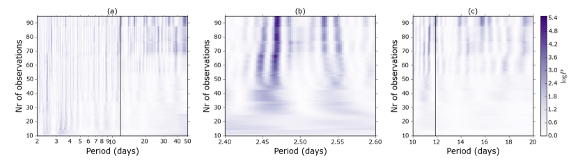
Figure 6.— Stacked periodograms of the HARPS-N RV observations, showing the evolution of the dataset as we gathered the observations. Each panel spans the following period range: (a) 2 to 50 days, (b) zoom-in around 2.5 days, and (c) from 10 to 20 days. The color scale, equal for all three panels represents the periodogram power. Note that the orbital period (marked by the vertical black line) is at $11.8728787$ $\pm$ $0.0000085$ days and the stellar rotation period is 13.6 $\pm$ 1.4 days.

Stacked periodograms

Figure 6 shows the evolution in the Bayesian Generalised Lomb-Scargle periodograms of the RVs as we add more observations (Mortier et al., 2015; Mortier & Collier Cameron, 2017). After about 50 observations we begin to see clear power at the orbital period of Kepler-1655b (11.8 days). We note that this is not the only or the most prominent feature in the periodograms. We also see several streaks of power in the region of 14 to 16 days. This broad range of periods, centered at the rotation period (13.6 days) is consistent with the relatively short-lived, phase-changing incoherent signatures of magnetic activity. We note that these signals are convolved with the window function of the observations, which contains many peaks ranging from about 10 to 50 days (panel (d) of Figure 7).

Periodicities near 2.5 and 3.2 days

We see strong peaks in the periodograms at periods of 2.5 and 3.2 days. We computed the 99% and 99.9% false alarm probability levels via bootstrapping and found that both levels lie well above the highest peaks in the periodograms of both the RV observations and the RV residuals. These signals are therefore not statistically significant. Since we do not have any other information about their nature we did not investigate them any further.

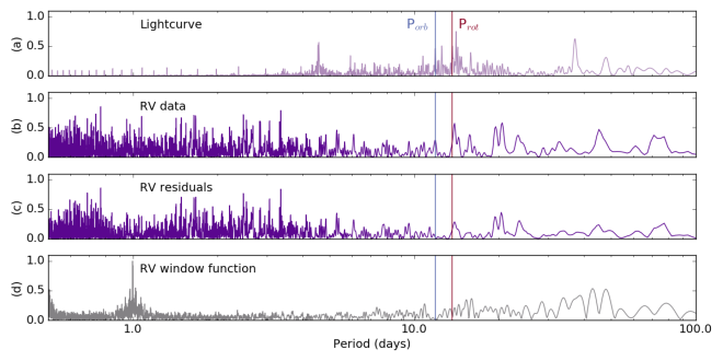
Figure 7.— Lomb-Scargle periodograms of: (a) the Kepler PDCSAP light curve; (b) the HARPS-N RV campaign; (c) the residuals from the RV fit to the HARPS-N observations; and (d) the window function of the RV campaign. None of the peaks in the periodograms of RV observations and residuals are statistically significant (the 99% false alarm probability levels are higher than the maximum power plotted).

6.3. Choice of RV model and priors

Table 1Parameters modeled in the RV analysis and their prior probability distributions.

Orbital period (from transits)	$P$	Gaussian ($11.8728787$, $0.0000085$)
Transit ephemeris (from transits)	$t_{\rm 0}$	Gaussian ($2455013.89795$, $0.00069$)
RV semi-amplitude	$K$	Uniform [0, $\infty$]
Orbital eccentricity	$e$	Uniform [0, 1]
Argument of periastron	$\omega$	Uniform [$0,2\pi$]
Amplitude of covariance	$\eta_{1}$	Uniform [0, $\infty$]
Evolution timescale (from ACF)	$\eta_{2}$	Gaussian ($23,8$)
Recurrence timescale (from ACF)	$\eta_{3}$	Gaussian ($13.6,1.4$)
Structure parameter	$\eta_{4}$	Gaussian (0.5, 0.05)
Uncorrelated noise term	$\sigma_{\rm s}$	Uniform [0, $\infty$]
Systematic RV offset	$RV_{0}$	Uniform

For the Gaussian priors, the terms within parentheses represent the mean and standard deviation of the distribution. The terms within square brackets stand for the lower and upper limit of the specified distribution; if no interval is given, no limits are placed.

In light of these preliminary investigations, we choose to stay open to the possible presence of correlated RV noise arising from Kepler-1655’s magnetic activity. We take any such variations into account via Gaussian-process (GP) regression. Our approach is very similar to that of López-Morales et al. (2016). The GP is encoded by a quasi-periodic kernel of the form:

$$k(t,t^{\prime})=\eta_{1}^{2}\,\cdot\,\exp\left[-\frac{(t-t^{\prime})^{2}}{2\,\eta_{2}^{2}}-\frac{2\,\sin^{2}\left(\frac{\pi(t-t^{\prime})}{\eta_{3}}\right)}{\eta_{4}^{2}}\right].$$ (1)

The hyperparameter ${\eta_{1}}$ is the amplitude of the correlated noise; $\eta_{2}$ corresponds to the evolution timescale of features on the stellar surface that produce activity-induced RV variations; $\eta_{3}$ is equivalent to the stellar rotation period; and $\eta_{4}$ gives a measure of the level of high-frequency structure in the GP model.

$\eta_{2}$ and $\eta_{3}$ are constrained with Gaussian priors using the values for the stellar rotation period and the active-region lifetime determined via the ACF analysis described in Section 6.2.

We constrain $\eta_{4}$ with a Gaussian prior centered around 0.5 $\pm$ 0.05. This value, which is adopted based on experience from previous datasets (including CoRoT-7 Haywood et al. (2014), Kepler-78 Grunblatt et al. (2015) and Kepler-21 López-Morales et al. (2016)), allows the RV curve to have up to two or three maxima and minima per rotation, as is typical of stellar light curves and RV curves (see Jeffers et al. (2009)). Foreshortening and limb darkening act to smooth stellar photometric and RV variations, which means that a curve with more than 2-3 peaks per rotation cycle would be unphysical.

The strong constraints on the hyperparameters (particularly $\eta_{4}$) are ultimately incorporated into the likelihood of our model, and as shown in Figures 8 and 9 provide a realistic fit to the activity-induced variations. We note that GP regression, despite being robust is also extremely flexible. Our aim is not to test how well an unconstrained GP can fit the data, but rather to constrain it to the maximum of our prior knowledge, in order to account for activity-driven signals as best as we can.

We account for the potential presence of uncorrelated, Gaussian noise by adding a term $\sigma_{\rm s}$ in quadrature to the RV error bars provided by the DRS.

We model the orbit of Kepler-1655b as a Keplerian with free eccentricity. We adopt Gaussian priors for the orbital period and transit phase, using the best-fit values for these parameters estimated in Section 5. Finally, we account for the star’s systemic velocity and the instrumental zero-point offset of the HARPS-N spectrograph with a constant term $RV_{0}$. We summarize the priors used for each free parameter of our RV model in Table 1.

The covariance kernel of Equation 1 is used to construct the covariance matrix K, of size $n$ x $n$ where $n$ is the number of RV observations. Each element of the covariance matrix tells us about how much each pair of RV data are correlated with each other.

For a dataset $\underline{y}$ (with $n$ elements $y_{i}$), the likelihood $\mathcal{L}$ is calculated as (Rasmussen & Williams, 2006):

$$\log\mathcal{L}=-\frac{n}{2}\log(2\pi)-\frac{1}{2}\log(|{\bf K}+\sigma_{i}^{2}\,{\bf I}|)$$ (2)

$$-\frac{1}{2}\,\underline{y}^{T}.\,({\bf K}+\sigma_{i}^{2}\,{\bf I})^{-1}.\,\underline{y}.$$

The first term is a normalisation constant. The second term, where $|{\bf K}|$ is the determinant of the covariance matrix, acts to penalise complex models. The third term represents the $\chi^{2}$ of the fit. The white noise component, $\sigma_{i}$, includes the intrinsic variance of each observation (i.e. the error bar, see Table 4) and the uncorrelated Gaussian noise term $\sigma_{s}$ mentioned previously, added together in quadrature. ${\bf I}$ is an identity matrix of size $n$ x $n$.

We maximize the likelihood of our model and determine the best-fit parameter values through a MCMC procedure similar to the one described in Haywood et al. (2014), in an affine-invariant framework (Goodman & Weare, 2010).

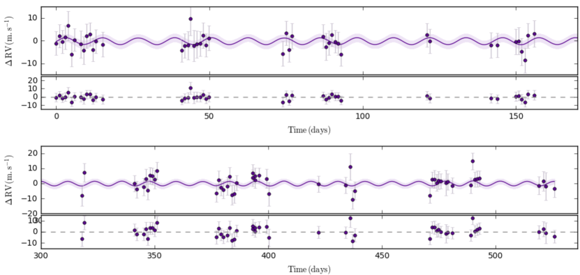
Figure 8.— The HARPS-N RV data (points with error bars) and our best fit (dark line with light-shaded 1-$\sigma$ error regions): (top) zoom-in on the first season; (bottom) zoom-in on the second season, the following year. The residuals after subtracting the model from the data (in m.s^-1) are shown in the plots below each fit.

6.4. Underlying assumptions in our choice of covariance kernel

In imposing strong priors on ${\eta_{2}}$ and ${\eta_{3}}$, we are making the assumption that the rotation period $P_{\rm rot}$ and active-region lifetime $\tau_{\rm ev}$ are the same in both the photometric light curve and the RV curve. This is potentially not the case, as the photometric and spectroscopic variations may be driven by different stellar surface markers/phenomena (eg. starspots, faculae). They may rotate at different speeds, be located at significantly different latitudes on the stellar surface or have very different lifetimes. Faculae on the Sun persist longer than spots. They are likely the dominant contributors to the RV signal, while the shorter-lived spots will dominate the photometry.
It is difficult to check the validity of this assumption as these very same factors also impede our ability to determine precise estimates for $P_{\rm rot}$ and $\tau_{\rm ev}$, particularly in RV observations for which we do not benefit from long-term, high-cadence sampling. For example, the rotation period usually appears in the periodograms (of the light curve and the RVs) as a forest of peaks rather than a single clean, sharp peak (see Figure 7). This effect is the result of the tracers (spots, faculae, etc.) having lifetimes of just a few rotations, and subsequently reappearing at different longitudes on the stellar surface. This scrambles the phase and thus modulates the period; see Section 6.2.

6.5. Results of the RV fitting

We investigated the effect of including a GP and/or an uncorrelated noise term on the accuracy and precision of our mass determination for Kepler-1655b. We also looked at the effects of using different priors for $\eta_{2}$ and $\eta_{3}$, and injecting a fake planet with the density of Earth.

Table 2Effects of including correlated and/or uncorrelated noise contributions in our RV fitting.

	$K$	$\eta_{1}$	$\sigma_{\rm s}$
	[m.s-1]	[m.s-1]	[m.s-1]
(a) Original RV dataset
Model 1	1.47 $\pm^{0.88}_{0.80}$	1.6 $\pm^{1.3}_{1.0}$	4.3 $\pm$ 0.8
Model 2	1.46 $\pm^{0.81}_{0.74}$	-	4.6 $\pm$ 0.9
Model 3	1.51 $\pm^{0.47}_{0.46}$	-	-
(b) RV dataset with injected Earth-composition Kepler-1655b
Model 1	6.13 $\pm^{0.90}_{0.93}$	1.8 $\pm^{1.3}_{1.1}$	4.4 $\pm^{0.9}_{0.8}$
Model 2	6.19 $\pm^{0.83}_{0.84}$	-	4.6 $\pm^{0.9}_{0.7}$
Model 3	6.25 $\pm$0.48	-	-

Model 1: correlated & uncorrelated noise (GP, $\sigma_{\rm s}$, $RV_{0}$ and a Keplerian orbit); Model 2: uncorrelated noise ($\sigma_{\rm s}$, $RV_{0}$ and a Keplerian orbit); Model 3: no noise components ($RV_{0}$ and a Keplerian orbit). (b): we injected a Keplerian signal with semi-amplitude 6.2 m.s^-1 (after subtracting the detected amplitude of 1.47 m.s^-1), corresponding to a mass of 22.6 M_⊕.

We tested three models accounting for both correlated and uncorrelated noise. The first one, which we refer to as Model 1, contains both correlated and uncorrelated noise, in the form of a GP and a term $\sigma_{\rm s}$ added in quadrature to the errors bars, respectively. In addition, the model has a term $RV_{0}$ and a Keplerian orbit. The second model we tested (Model 2) has no GP but does account for uncorrelated noise via a term $\sigma_{\rm s}$ added in quadrature to the error bars. Again, the model also has a term $RV_{0}$ and a Keplerian orbit. Our third and simplest model (Model 3) contains no noise components at all. It only contains a zero offset $RV_{0}$ and a Keplerian orbit.

For all models, we used the same prior values and 1-$\sigma$ uncertainties for all the timescale parameters (orbital $P$ and $t_{0}$, stellar $P_{\rm rot}$ and $\tau_{\rm ev}$) as well as the structure hyperparameter $\eta_{4}$. We found that the eccentricity and argument of periastron remained the same in all cases (consistent with a circular orbit). The zero offset $RV_{0}$ was also unaffected. The best-fit values for the remaining parameters ($K$, $\eta_{1}$, $\sigma_{\rm s}$) for each model tested are reported in Table 2.

Table 3System Parameters for the Kepler-1655 system.

Parameter	Value	Source
RA [h m s]	19 06 45.44	a
DEC [d m s]	+39 12 42.63	a
Spectral type	G0V
$m_{V}$	11.05$\pm$0.08	a
$B-V$	0.57	a
Parallax [mas]	4.34$\pm$ 0.53	b
Distance [pc]	230.41$\pm$ 28.14
$T_{\rm eff}$ [K]	6148$\pm$ 71	c
$\log{g}$	4.36$\pm$ 0.10	c
${\rm[Fe/H]}$	$-$0.24$\pm$ 0.05	c
$\Delta\nu$ [$\mu$Hz]	128.8$\pm$ 1.3	d
$\nu_{max}$ [$\mu$Hz]	2928.0$\pm$ 97.0	d
Mass $[M_{\odot}]$	1.03$\pm$ 0.04	e
Radius $[R_{\odot}]$	1.03$\pm$ 0.02	e
$\rho_{\ast}$ [$\rho_{\odot}$]	0.94$\pm$ 0.04
Age [Gyr]	2.56$\pm$1.06	e
$v\,\sin{i}$ [km s-1]	3.5$\pm$ 0.5	d
Limb darkening $q_{1}$	$0.403$ $\pm$ $0.077$	f
Limb darkening $q_{2}$	$0.260$ $\pm$ $0.039$	f
$<\log{R^{\prime}_{\rm HK}}>$	$-$4.97	g
Prot [days]	$13.6$ $\pm$ $1.4$	f
$\tau_{\rm ev}$ [days]	$23$ $\pm$ $8$	f
Transit and radial-velocity parameters
Orbital period $P$ [days]	$11.8728787$ $\pm$ $0.0000085$	f
Time of mid-transit $t_{0}$ [BJD]	$2455013.89795$ $\pm$ 0.00069	f
Radius ratio $(R_{b}/R_{\star})$	$0.01965$ $\pm$ $0.00069$	f
Orbital inclination $i$ [deg]	$87.62$ $\pm$ $0.55$	f
Transit impact parameter $b$	$0.85$ $\pm$ $0.13$	f
RV semi-amplitude $K$ [m.s-1]	$1.47$ $\pm$ ${}^{0.88}_{-0.80}$	g
RV semi-amplitude 68% (95%) upper limit [m.s-1]	$<1.8$ ($<2.8$)	g
Eccentricity 68% (95%) upper limit	$<0.36$ ($<0.79$)	g
Argument of periastron $\omega_{p}$ [deg]	-71 $\pm$ 92	g
RV offset RV0 [km.s-1]	-40.6386 $\pm$ 0.000006	g
Derived parameters for Kepler-1655b
Radius $R_{b}$ [R⊕]	$2.213$ $\pm$ $0.082$	e,f
Mass $M_{b}$ [M⊕]	$5.0$ $\pm$ ${}^{3.1}_{-2.8}$	e,f,g
Mass 68% (95%) upper limit [M⊕]	$<6.2$ ($<10.1$)	e,f,g
Density $\rho_{b}$ [g.cm-1]	$2.5$ $\pm$ ${}^{1.6}_{-1.4}$	e,f,g
Density 68% (95%) upper limit [g.cm-1]	$<3.2$ ($<5.1$)	e,f,g
Scaled semi-major axis $a/R_{\star}$	$20.5$ $\pm$ $4.1$	f
Semi-major axis $a_{b}$ [AU]	0.103 $\pm$ 0.001	f, g
Incident flux $F$ [F⊕]	$155$ $\pm$ $7$	e,f

Overall, the value of the RV semi-amplitude of Kepler-1655b is robust to within 5 cm.s^-1, regardless of whether we account for (un)correlated noise or not. This is a reflection of the fact that the host star has fairly low levels of activity. When the GP is included, its amplitude $\eta_{1}$ is similar to that of $K$. However, we note that the uncorrelated noise term is large and dominates both the GP and the planet Keplerian signal. This may be a combination of additional instrumental noise (the star is very faint and our observations are largely dominated by photon noise) and short-term granulation motions. Also, rotationally-modulated activity signals that were sampled too sparsely may also appear to be uncorrelated and be absorbed by this term rather than the GP (as was likely the case in López-Morales et al. (2016)).

Regardless of its nature, we cannot ignore the presence of uncorrelated noise. Doing so would lead us to underestimating our 1-$\sigma$ uncertainty on $K$ by 40%. Finally, we see that when we go from Model 2 (uncorrelated noise only) to Model 1 (correlated and uncorrelated noise), the uncertainty on $K$ increases by about 7 cm.s^-1. We attribute this slight inflation to the fact that the orbital period of Kepler-1655b is close to the rotation period of its host star. This acts to incorporate this proximity of orbital and stellar timescales in the mass determination of Kepler-1655b.

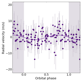
Figure 9.— Phase plot of the orbit of Kepler-1655b for the best-fit model after subtracting the Gaussian-process component.

6.5.1 Effects of varying $P_{\rm rot}$ and $\tau_{\rm ev}$

We ran models with different values for the stellar rotation and evolution timescales ($P_{\rm rot}$ ranging between 11-20 days, $\tau_{\rm ev}$ ranging between 13-50 days, with associated uncertainties ranging from 1-8 days for both). We found that the amplitude of the GP and its associated uncertainty remained the same throughout our simulations. The semi-amplitude of Kepler-1655b also remained the same to within 10%, ranging between 1.37-1.47 m.s^-1, with a 1-$\sigma$ uncertainty ranging from 0.85-0.90 m.s^-1. The uncertainty was largest in cases with the longest evolution timescale (i.e., the activity signals are assumed to retain coherency for a long time) and when the rotation period overlapped most with the orbital period of Kepler-1655b (at 11 days).

6.5.2 RV signature of Kepler-1655b if it had an Earth-like composition

We subtracted a Keplerian with a semi-amplitude $K$ of 1.47 m.s^-1, corresponding to that of Model 1, and subsequently injected a Keplerian signal with semi-amplitude 6.2 m.s^-1, i.e. a mass of 22.6 M_⊕(at the period and phase of Kepler-1655b). With Kepler-1655b’s radius of 2.213 R_⊕and according to the composition models of Zeng et al. (2016), these mass and radius values correspond to an Earth-like composition. We tested all three Models after injecting this artificial signal. As shown in panel (b) of Table 2, we see a completely consistent behavior when the semi-amplitude of the planet is artificially boosted. In particular, the amplitude $\eta_{1}$ of the GP remains consistent well within 1-$\sigma$. This artificial signal is detected at high significance (7-$\sigma$). This test confirms that if the planet had an Earth-like composition, our RV observations would have been sufficient to determine its mass with accuracy and precision; it therefore shows that Kepler-1655b must contain a significant fraction of volatiles. We find that only 0.014% of the samples in our actual posterior mass distribution lie at or above 22.6 M_⊕, and therefore conclude that we can significantly rule out an Earth-like composition for this planet.

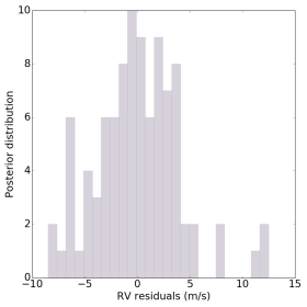
Figure 10.— Histogram of the residuals of the RVs, after subtracting Model 1 from the data. The residuals are close to Gaussian-distributed.

6.6. Mass and composition of Kepler-1655b

The RV fit from Model 1, which we adopt for our mass determination, is plotted in Figure 8. The corresponding correlation plots for the parameters in the MCMC run, attesting of its efficient exploration and good convergence, are shown in the Appendix. The residuals, shown as a histogram in Figure 10 are Gaussian-distributed. The phase-folded orbit of Kepler-1655b is shown in Figure 9.

Taking the semi-amplitude obtained from Model 1, we determine the mass of Kepler-1655b to be 5.0$\pm^{3.1}_{2.8}$ M_⊕. The posterior distribution of the mass is shown in Figure 11. For comparison, we also show the posterior distribution obtained after we injected the artificial signal corresponding to a Kepler-1655b  with an Earth-like composition. As we discussed in Section 6.5.2, we see that the two posterior distributions are clearly distinct and with little overlap. Despite the low significance of our planet mass determination, we can state with high confidence that Kepler-1655b  has a significant gaseous envelope and is not Earth-like in composition. The mass of Kepler-1655b  is less than 6.2   M_⊕  at 68% confidence, and less than 10.1  M_⊕  at 95% confidence. Our analysis excludes an Earth-like composition with more than 98% confidence (see Section 6.5.2).

We obtain a bulk density for Kepler-1655b of $\rho_{b}=2.5\pm^{1.6}_{1.4}$ g.cm^-3. The planet’s density is less than 3.2 g.cm^-3 to 68% confidence and less than 5.1 g.cm^-3 to 95% confidence.

The planet may have experienced some moderate levels of evaporation, which may be significant if its mass is indeed below 5 M_⊕.

The eccentricity is consistent with a circular orbit and with the constraints derived from our asterodensity profiling analysis (Section 5.1). At an orbital period of 11.8 days, we do not expect this planet to be tidally circularized.

The large uncertainty on our mass determination is not unexpected. First, the host star is fainter than typical HARPS-N targets ($m_{V}=11.05$) so our RV observations are photon-limited. Second, the window function of the RV observations contains a number of features in the 10-50 day range (see panel (d) of Figure 7 and Section 6.2.1), which implies that the stellar rotation period, close to 14 days, is sampled rather sparsely. Any activity-induced RV variations, which can reasonably be expected at the level of 1-2 m.s^-1 from suppression of convective blueshift in facular areas, will thus be sparsely sampled; this is likely to wash out their correlated nature and will result in additional uncorrelated noise – which in turn inflates the uncertainty of our mass determination.

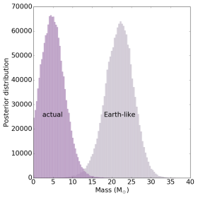
Figure 11.— Posterior distributions of the mass parameter: “actual” refers to the posterior distribution obtained when fitting Model 1 to the actual RV data, while “Earth-like” is the distribution we obtain if we inject a planet of Earth-like composition with Kepler-1655b’s 2.2 R_⊕ radius. Such a planet would have a mass of $\approx$ 22.6M_⊕.

7. Discussion: Kepler-1655b among other known exoplanets

With a radius of 2.213 R_⊕  and a mass less than 10.1 M_⊕  (at 95% confidence), Kepler-1655b  straddles the region between small, rocky worlds and larger, gas-rich worlds. Figure 12 shows the place of Kepler-1655b as a function of mass and radius, alongside other well-characterized exoplanets in the 0.1–32 M_⊕  and 0.3–8 R_⊕  range. The exoplanets that are shown have measured masses and were taken from the list compiled by Christiansen et al. (2017). We used radius measurements from Fulton et al. (2017) where available, or extracted them from the NASA Exoplanet Archive otherwise. We include the planets of the solar system, with data from the NASA Goddard Space Flight Center archive. We overplot the planet composition models of Zeng et al. (2016).

For the purpose of the present discussion, we identify and highlight the planets that have a strong likelihood of being gaseous (in blue) and rocky (in red). For each planet, we drew 1000 random samples from a Gaussian distribution centered at the planet mass and radius, with a width given by their associated mass and radius 1-$\sigma$ uncertainties. Planets whose mass and radius determinations indicate a 96% or higher probability of lying above the 100% H₂O line are colored in blue. Planets that lie below the 100% MgSiO₃ line with 96% probability or higher, and have a probability of less than 4% of lying above the 100% H₂O line are colored in red. All other planets, colored in gray, are those that do not lie on either extreme of this probability distribution (even though their mass and radius measurement uncertainties may be smaller than others that we identified as rocky or gaseous). For clarity we omitted their error bars on this plot.

We note that Kepler-1655b, shown in purple is one of these intermediate worlds.

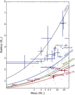
Figure 12.— Mass-radius diagram for planets in the 0.1–32 M_⊕and 0.3–8 R_⊕ranges. The blue points correspond to “gas-rich” planets, while the red points represent planets that are very likely to be rocky in composition (see Section 7). The planets that fall in neither category are colored in gray, and their error bars are omitted for clarity. Kepler-1655b  and its associated 1-$\sigma$ measurement uncertainties are shown in purple.

For this discussion, we define “water worlds” as planets for which the majority of their content (75-80% in terms of their radius) is not hydrogen. Their densities indicate that they must have a significant non-rocky component, but this component is water rather than hydrogen. They formed from solids with high mean molecular weight. We refer to planets with a radius fraction of hydrogen to core that is greater than 20% as “gaseous worlds”.

We wish to investigate how gaseous planets (lying above the water line) behave as a function of planet radius and incident flux received at the planet surface as compared to their rocky counterparts. For this purpose, we created the three plots shown in Figure 13, in which planets are again displayed as probability density distributions rather than single points with 1-$\sigma$ uncertainties. For each planet, we draw 1000 random samples from a Gaussian distribution centered at the planet radius and incident flux measurements, with a width given by their associated 1-$\sigma$ uncertainties. We display the resulting distributions as a two-dimensional binned density plot so that the regions of higher probability appear darker.

In panel (a), we show the resulting density distribution for planets that we previously identified as rocky worlds – over 96% of the Gaussian draws fall below the MgSiO₃ line and fewer than 4% fall above the the H₂O line. In panel (b), we show the density distribution for planets that we previously identified as gaseous worlds – over 96% of the Gaussian draws fall above the H₂O line. In both panels (a) and (b), we plot the well-characterized sample described earlier in the discussion (planets with mass determinations listed in Christiansen et al. (2017), and radius and incident flux measurements from Fulton et al. (2017) or the NASA Exoplanet Archive). We include the planets of the solar system. We label the planets of the solar system and the planets responsible for some of the more prominent features, as well as the position of Kepler-1655b  to guide the reader. In panel (c), we show all 2025 planets with updated radii and incident fluxes from the CKS survey (Fulton et al., 2017). The labels for the solar system planets, LHS1140b and Kepler-4b are included to facilitate comparison with panels (a) and (b).

As has been noted in previous works including Weiss & Marcy (2014); Wolfgang et al. (2016); Jontof-Hutter et al. (2016), we see a great diversity of masses for small, rocky planets (see Figure 13a). They are also present in a broad range of incident fluxes (from $<1$ F_⊕ up to 10,000 F_⊕). Gas-dominated planets also span a wide range of masses, but seem to occur in a narrower range of incident fluxes (see Figure 13b). Both rocky and gaseous planets at longer orbital periods, and thus low incident fluxes (below a few F_⊕) are more difficult to detect and characterize; this means that our exoplanet sample is most likely incomplete in this flux range. We note that Figure 13 is not corrected for any such observational biases. Planets at very high incident fluxes, however, are easiest to detect as they are in very close orbits. We note that the known population of hot Jupiters, at large radius and extremely high incident flux (up to 10,000 F_⊕) is not represented in these plots; however, previous studies have shown that at the high end of the radius distribution, the hot Jupiters have so much gas that they keep most of it, even in highly-irradiated orbits.

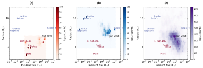
Figure 13.— Incident flux as a function of radius for well-characterized planets to date. In all three panels, each planet is represented as a probability-distribution “cloud” (see main text for details). Panel (a): density distribution for planets that are likely rocky, i.e. with $>$ 96% probability of lying below the 100% MgSiO₃ line, and $<$ 4% probability of lying above the 100% H₂O line. Panel (b): density distribution for planets identified as gas-rich, i.e. with $>$ 96 % probability of lying above the 100% H₂O line. Panel (c): all planets from the CKS sample (Fulton et al., 2017), including those without a mass determination. Both the evaporation valley and evaporation desert are apparent.

In panel (c) of Figure 13, we see the evaporation valley between 1.5 and 2 R_⊕  that was recently observed by Fulton et al. (2017) (see also Zeng et al. (2017)) and predicted theoretically by Owen & Wu (2017) and Jin & Mordasini (2017).

At intermediate radii, Figure 13c shows a dearth of planets at the highest incident fluxes with radii $\sim$ 2-4 R_⊕. It has been shown to be unlikely to be dominated by observational biases, and is commonly referred to as the evaporation desert or sub-Neptune desert (Sanchis-Ojeda et al., 2014; Lundkvist et al., 2016).

Planets in this region either do not exist or they are extremely rare. Perhaps it is a transition region, and they will exist in this region but only for a very short time, making them very difficult to detect.

The evaporation desert leads us to speculate on the composition of Neptune-size planets, and their formation and migration histories. Models of planet interiors are limited by degeneracies in composition for a given mass and radius, regardless of how precisely these two observables may be determined (Rogers & Seager, 2010). This is especially an issue for planets with sizes in the super-Earth to small Neptune range. The very existence of the evaporation desert and the evaporation valley argues against a very water-rich population. Water worlds would survive in close-in, highly-irradiated orbits; they could lose their H/He envelopes through evaporation, but the majority of their steam envelopes would remain, so they would never be stripped down to bare rock (Lopez, 2016). However, further studies need to be carried out to understand exactly how strong these constraints are.

On one hand, the distribution of highly-irradiated, low-mass planets is mainly shaped by formation processes, such as whether most planets form before their disks dissipate. On the other hand, it may be that they are shaped by evolution processes, such as evaporation. Lopez & Rice (2016) show that constraining the slope of the rocky/non-rocky transition (the edge of the evaporation valley) can differentiate between these two scenarios.

Kepler-1655b falls in the midst of this transition region, and is in an orbit where the irradiation levels start to be high enough that it is in a relatively unpopulated zone. It is therefore part of a population of planets that we should actively seek to characterize further.

8. Conclusions

We confirm the planetary nature of Kepler-1655b, characterize its host star and determine its radius and mass.

Our main conclusions are:

• Kepler-1655b  is a moderately-irradiated (F = 155 $\pm$ 7 F_⊕), sub-Neptune with a substantial gas envelope. We measure its radius to be 2.213$\pm$0.082 R_⊕, and determine its mass to be 5.0$\pm^{3.1}_{2.8}$  M_⊕, or less than 10.1 M_⊕  at 95% confidence. This places Kepler-1655b  in a still relatively unexplored area of parameter space, where it straddles the observed evaporation valley between small, rocky planets and Neptune-size, gaseous worlds (Fulton et al., 2017; Owen & Wu, 2017; Jin & Mordasini, 2017). In addition, its moderately-irradiated orbit places it close to the observed evaporation desert (Sanchis-Ojeda et al., 2014; Lundkvist et al., 2016).

• The host star Kepler-1655  is a G0V Sun-like star with a rotation period of $13.6\pm 1.4$ days. The magnetic activity behavior that we observe in both our photometric and spectroscopic time series are similar to those of the Sun in its quieter phase. We see the occasional emergence of active regions with average lifetimes of $23\pm 8$ days, as measured from the Kepler photometric curve via an autocorrelation analysis. We measure activity-driven radial-velocity variations with an RMS of 0.5 m.s^-1. This value is consistent with ongoing HARPS-N observations of the Sun as a star, that display an RMS of 1.6 m.s^-1 even though the Sun is now entering the low phase of its 11-year magnetic activity cycle (see Dumusque et al. (2015) and Phillips et al., in prep.). Our findings are also consistent with activity levels of order 1-2 m.s^-1 seen in the quietest main-sequence, Sun-like stars in spectroscopic surveys (eg. Isaacson & Fischer (2010); Motalebi et al. (2015)).

• In the Kepler-1655  system, the radial-velocity RMS induced by magnetic activity, even though it is a relatively quiet star, is of comparable magnitude to the orbital reflex motion induced by the planet Kepler-1655b. We account for activity variations as both correlated and uncorrelated noise to obtain an accurate (though not necessarily precise) planetary mass determination. In agreement with previous studies (eg. López-Morales et al. (2016); Rajpaul et al. (2015)), we see that the precision of our mass determination depends crucially on regular and adequate sampling of the stellar rotation timescale. If the activity signals are sampled too sparsely, their correlation structure will be changed or lost, in which case they will be best accounted for through an uncorrelated, Gaussian noise term; this will in turn inflate the uncertainty associated with our mass determination.

• It is difficult to measure rotation periods accurately, as they can be different at different levels of activity, likely because the stellar surface is dominated by different types of active regions (eg. faculae, spots). For this reason, extra care must be taken in radial-velocity analyses, particularly in systems such as Kepler-1655, where the stellar rotation ($13.6\pm 1.4$ days) and planetary orbital period (11.8728787$\pm$0.0000085 days) are close to each other.

In order to robustly constrain our planet formation models and look into the details of all these scenarios and processes, we require mass determinations that are accurate and reliable. It is especially important that we focus our characterization efforts on planets like Kepler-1655b  that straddle observational boundaries, such as the evaporation valley between gaseous and rocky planets and the evaporation desert at high irradiation levels. Determining the masses of planets like Kepler-1655b is a necessary step to building a statistical sample that will feed models of planetary formation and evolution.

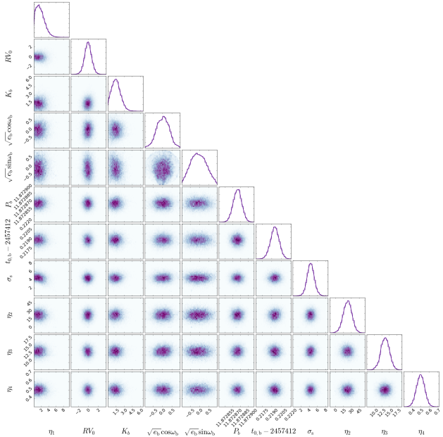
Figure 14.— Marginalized 1- and 2-D posterior distributions of the RV model parameters output from the MCMC procedure. The solid lines overplotted on the histograms are kernel density estimations of the marginal distributions. The smooth, Gaussian-shaped posterior distributions attest of the good convergence of the MCMC chains.

Table 4HARPS-N RV observations and spectroscopic activity indicators, determined from the DRS. From left to right are given: barycentric Julian date BJD, radial-velocity $RV$, the estimated 1-$\sigma$ uncertainty on the RV ($\sigma_{RV}$), the full width at half-maximum ($FWHM$), contrast and line bisector of ($BIS$) of the cross-correlation function (as defined in Queloz et al. (2001)), the Ca II activity indicator $\log R^{\prime}_{HK}$ and its 1-$\sigma$ uncertainty $\sigma_{\log R^{\prime}_{HK}}$.

Barycentric Julian Date	RV	$\sigma_{RV}$	FWHM	contrast	BIS	$\log R^{\prime}_{HK}$	$\sigma_{\log R^{\prime}_{HK}}$
[UTC]	[km.s-1]	[km.s-1]	[km.s-1]		[km.s-1]
2457180.523500	-40.63968	0.00270	7.86870	29.321	0.02594	-4.9614	0.0157
2457181.527594	-40.63651	0.00236	7.86380	29.310	0.02474	-4.9651	0.0128
2457182.603785	-40.63892	0.00259	7.86953	29.305	0.02778	-4.9600	0.0147
2457183.494217	-40.63709	0.00281	7.86066	29.369	0.04133	-4.9601	0.0161
2457184.498702	-40.63199	0.00463	7.85989	29.256	0.03136	-4.9596	0.0354
2457185.495085	-40.64455	0.00293	7.87730	29.309	0.03152	-4.9532	0.0178
2457186.572836	-40.63822	0.00226	7.86260	29.343	0.02592	-4.9750	0.0118
2457188.501974	-40.64006	0.00396	7.88033	29.250	0.03398	-4.9270	0.0263
2457189.492822	-40.64273	0.00415	7.86784	29.305	0.03193	-4.9742	0.0319
2457190.506147	-40.63649	0.00296	7.85754	29.330	0.01650	-4.9878	0.0207
2457191.506484	-40.63570	0.00232	7.87102	29.344	0.02833	-4.9906	0.0132
2457192.503233	-40.64261	0.00240	7.85594	29.332	0.03865	-4.9884	0.0140
2457193.506439	-40.63887	0.00259	7.86547	29.344	0.02939	-4.9654	0.0137
2457195.618836	-40.64015	0.00320	7.85577	29.331	0.02057	-4.9571	0.0206
2457221.430559	-40.64291	0.00239	7.86913	29.361	0.02674	-4.9743	0.0133
2457222.435839	-40.64084	0.00301	7.87471	29.314	0.02747	-4.9653	0.0191
2457223.460747	-40.64063	0.00449	7.88822	29.216	0.03258	-5.0076	0.0397
2457224.390932	-40.62888	0.00576	7.86308	29.208	0.04897	-4.9174	0.0493
2457225.433813	-40.64082	0.00533	7.87820	29.198	0.02494	-5.0425	0.0564
2457226.408684	-40.64007	0.00408	7.86647	29.256	0.01841	-4.9618	0.0324
2457227.450637	-40.63983	0.00331	7.84180	29.309	0.03703	-4.9530	0.0217
2457228.410287	-40.63623	0.00341	7.87077	29.293	0.02768	-4.9568	0.0214
2457229.429739	-40.64052	0.00274	7.86533	29.298	0.03706	-4.9567	0.0156
2457230.406112	-40.63739	0.00323	7.87646	29.312	0.02833	-4.9308	0.0203
2457254.397788	-40.64424	0.00323	7.85502	29.314	0.02396	-4.9604	0.0213
2457255.500146	-40.63523	0.00299	7.86901	29.308	0.02114	-4.9755	0.0184
2457256.421107	-40.64243	0.00309	7.87620	29.285	0.02475	-5.0159	0.0213
2457257.482828	-40.63653	0.00335	7.87228	29.271	0.01542	-4.9738	0.0229
2457267.507688	-40.63665	0.00275	7.87107	29.284	0.02316	-4.9523	0.0155
2457268.565339	-40.64117	0.00391	7.87216	29.272	0.02490	-4.9535	0.0286
2457269.463909	-40.63953	0.00294	7.88436	29.297	0.02912	-4.9824	0.0188
2457270.452464	-40.63594	0.00244	7.86921	29.341	0.03088	-4.9645	0.0127
2457271.453922	-40.63895	0.00217	7.86716	29.344	0.02627	-4.9705	0.0106
2457272.495252	-40.63976	0.00269	7.87068	29.289	0.03039	-4.9893	0.0161
2457273.471826	-40.64459	0.00263	7.86265	29.320	0.03018	-4.9924	0.0149
2457301.432438	-40.63609	0.00280	7.86113	29.327	0.01631	-5.0003	0.0171
2457302.432090	-40.63881	0.00300	7.86872	29.290	0.03184	-4.9895	0.0177
2457322.359064	-40.64060	0.00339	7.86850	29.200	0.03729	-4.9534	0.0215
2457324.381964	-40.64046	0.00310	7.85083	29.271	0.03889	-4.9723	0.0192
2457330.349610	-40.63902	0.00326	7.86853	29.288	0.01826	-4.9757	0.0214
2457331.372976	-40.63873	0.00400	7.84861	29.288	0.03181	-4.9975	0.0315
2457332.370233	-40.64343	0.00392	7.88092	29.280	0.03704	-4.9701	0.0289
2457333.372096	-40.64721	0.00328	7.87162	29.263	0.02773	-5.0009	0.0246
2457334.328880	-40.63632	0.00305	7.86380	29.304	0.02669	-4.9949	0.0201
2457336.372433	-40.63546	0.00371	7.87532	29.294	0.02301	-4.9793	0.0267
2457498.664041	-40.64669	0.00518	7.85834	29.142	0.00964	-4.9501	0.0413
2457499.669841	-40.63127	0.00428	7.85774	29.202	0.02395	-4.9950	0.0349
2457521.623607	-40.63859	0.00294	7.87430	29.328	0.03426	-4.9826	0.0181
2457522.593255	-40.64256	0.00331	7.85636	29.278	0.03021	-5.0042	0.0245
2457525.643222	-40.64070	0.00368	7.85232	29.286	0.04013	-4.9688	0.0257
2457526.666772	-40.63541	0.00447	7.85574	29.270	0.02673	-4.9869	0.0360
2457527.615676	-40.64328	0.00429	7.86272	29.214	0.03598	-4.9852	0.0342
2457528.632060	-40.63341	0.00328	7.86301	29.249	0.02537	-4.9359	0.0199
2457529.644972	-40.63372	0.00324	7.86321	29.255	0.02607	-4.9483	0.0205
2457530.649803	-40.63592	0.00418	7.85874	29.177	0.02875	-5.0283	0.0366
2457531.672726	-40.63028	0.00382	7.85133	29.244	0.01415	-4.9776	0.0283
2457557.640527	-40.64505	0.00403	7.84956	29.207	0.03445	-4.9784	0.0301
2457558.611395	-40.63639	0.00426	7.83640	29.255	0.03740	-4.9370	0.0298
2457559.640215	-40.64116	0.00355	7.87551	29.164	0.02475	-4.9554	0.0227
2457560.634300	-40.64283	0.00378	7.85731	29.167	0.02360	-4.9598	0.0255
2457562.593091	-40.64033	0.00377	7.86254	29.244	0.02591	-4.9733	0.0264
2457563.620948	-40.63391	0.00427	7.87441	29.158	0.04132	-4.9638	0.0310
2457564.607576	-40.64620	0.00472	7.84112	29.226	0.02182	-4.9581	0.0359
2457565.628463	-40.64556	0.00408	7.86775	29.249	0.02912	-4.9645	0.0290
2457566.630680	-40.63824	0.00246	7.87116	29.285	0.01880	-4.9889	0.0133
2457573.575425	-40.63182	0.00374	7.85929	29.305	0.02756	-4.9720	0.0264

Barycentric Julian Date	RV	$\sigma_{RV}$	FWHM	contrast	BIS	$\log R^{\prime}_{HK}$	$\sigma_{\log R^{\prime}_{HK}}$
[UTC]	[km.s-1]	[km.s-1]	[km.s-1]		[km.s-1]
2457573.597046	-40.63485	0.00329	7.86519	29.315	0.02634	-4.9879	0.0221
2457574.566779	-40.63346	0.00274	7.87878	29.312	0.02665	-4.9477	0.0149
2457574.586467	-40.63648	0.00278	7.86857	29.326	0.02920	-4.9623	0.0159
2457576.557217	-40.63311	0.00246	7.87205	29.311	0.02995	-4.9681	0.0128
2457579.629640	-40.63536	0.00430	7.85924	29.250	0.02335	-4.9734	0.0317
2457580.702970	-40.64565	0.00629	7.86485	29.182	0.02583	-4.9331	0.0533
2457602.492695	-40.63907	0.00306	7.85957	29.311	0.03089	-4.9285	0.0172
2457614.470313	-40.63970	0.00287	7.86161	29.292	0.03215	-4.9681	0.0165
2457616.518107	-40.62758	0.00751	7.84425	29.065	0.03880	-4.9471	0.0676
2457617.485597	-40.64913	0.00426	7.84666	29.192	0.03402	-4.9775	0.0325
2457618.483689	-40.64341	0.00402	7.86390	29.124	0.02040	-4.9969	0.0305
2457651.405471	-40.64647	0.00294	7.86796	29.302	0.02770	-4.9582	0.0171
2457652.404666	-40.63602	0.00277	7.87473	29.349	0.02870	-4.9674	0.0154
2457653.410155	-40.63573	0.00393	7.86262	29.305	0.02438	-4.9947	0.0298
2457654.408874	-40.63807	0.00344	7.86736	29.345	0.02750	-4.9921	0.0236
2457655.380684	-40.63649	0.00424	7.86868	29.252	0.02368	-4.9915	0.0327
2457656.400628	-40.63716	0.00251	7.85571	29.329	0.02444	-4.9617	0.0132
2457658.467841	-40.63825	0.00711	7.89902	29.261	0.02978	-5.0566	0.0775
2457659.409674	-40.63750	0.00321	7.86655	29.335	0.02576	-4.9494	0.0194
2457661.433530	-40.64007	0.00263	7.86886	29.389	0.02541	-4.9687	0.0146
2457669.401610	-40.63981	0.00268	7.87027	29.322	0.03286	-4.9664	0.0149
2457670.357039	-40.62378	0.00324	7.85478	29.319	0.02758	-4.9473	0.0196
2457671.396539	-40.63589	0.00260	7.87140	29.334	0.03001	-4.9790	0.0146
2457672.400889	-40.63547	0.00289	7.87136	29.313	0.02379	-4.9728	0.0174
2457673.332071	-40.63531	0.00276	7.86742	29.302	0.02206	-5.0001	0.0160
2457699.366303	-40.64003	0.00394	7.86373	29.291	0.03020	-4.9620	0.0266
2457701.363688	-40.63710	0.00480	7.85277	29.252	0.04106	-5.0048	0.0422
2457702.373816	-40.64049	0.00819	7.89468	29.016	0.03353	-4.8835	0.0685
2457706.345872	-40.64216	0.00357	7.87407	29.227	0.04043	-4.8960	0.0203

References

- Aigrain et al. (2015) Aigrain, S., Llama, J., Ceillier, T., et al. 2015, MNRAS, 450, 3211
- Baranne et al. (1996) Baranne, A., Queloz, D., Mayor, M., et al. 1996, Astronomy and Astrophysics Supplement Series, 119, 373
- Boisse et al. (2012) Boisse, I., Bonfils, X., & Santos, N. C. 2012, Astronomy and Astrophysics, 545, A109
- Borucki et al. (2011) Borucki, W. J., Koch, D. G., Basri, G., et al. 2011, ApJ, 736, 19
- Bressan et al. (2012) Bressan, A., Marigo, P., Girardi, L., et al. 2012, MNRAS, 427, 127
- Buchhave et al. (2016) Buchhave, L. A., Dressing, C. D., Dumusque, X., et al. 2016, AJ, 152, 160
- Campante et al. (2015) Campante, T. L., Barclay, T., Swift, J. J., et al. 2015, ApJ, 799, 170
- Christiansen et al. (2017) Christiansen, J. L., Vanderburg, A., Burt, J., et al. 2017, ArXiv e-prints, arXiv:1706.01892
- Claret & Bloemen (2011) Claret, A., & Bloemen, S. 2011, A&A, 529, A75
- Cosentino et al. (2012) Cosentino, R., Lovis, C., Pepe, F., et al. 2012, in Society of Photo-Optical Instrumentation Engineers (SPIE) Conference Series, Vol. 8446, Society of Photo-Optical Instrumentation Engineers (SPIE) Conference Series
- Coughlin & López-Morales (2012) Coughlin, J. L., & López-Morales, M. 2012, AJ, 143, 39
- da Silva et al. (2006) da Silva, L., Girardi, L., Pasquini, L., et al. 2006, A&A, 458, 609
- Dawson & Fabrycky (2010) Dawson, R. I., & Fabrycky, D. C. 2010, ApJ, 722, 937
- Dawson & Johnson (2012) Dawson, R. I., & Johnson, J. A. 2012, ApJ, 756, 122
- Diplas & Savage (1994) Diplas, A., & Savage, B. D. 1994, ApJS, 93, 211
- Dravins et al. (1981) Dravins, D., Lindegren, L., & Nordlund, A. 1981, A&A, 96, 345
- Dressing & Charbonneau (2015) Dressing, C. D., & Charbonneau, D. 2015, ApJ, 807, 45
- Dumusque et al. (2014) Dumusque, X., Boisse, I., & Santos, N. C. 2014, ApJ, 796, 132
- Dumusque et al. (2015) Dumusque, X., Glenday, A., Phillips, D. F., et al. 2015, ApJ, 814, L21
- Eastman et al. (2013) Eastman, J., Gaudi, B. S., & Agol, E. 2013, PASP, 125, 83
- Edelson & Krolik (1988) Edelson, R. A., & Krolik, J. H. 1988, ApJ, 333, 646
- Fossati et al. (2017) Fossati, L., Marcelja, S. E., Staab, D., et al. 2017, A&A, 601, A104
- Foukal (2004) Foukal, P. V. 2004, Solar Astrophysics, 2nd, Revised Edition, 480
- Fulton et al. (2017) Fulton, B. J., Petigura, E. A., Howard, A. W., et al. 2017, AJ, 154, 109
- Gaia Collaboration et al. (2016) Gaia Collaboration, Prusti, T., de Bruijne, J. H. J., et al. 2016, A&A, 595, A1
- Gelman & Rubin (1992) Gelman, A., & Rubin, D. B. 1992, Statistical science, 457
- Gettel et al. (2016) Gettel, S., Charbonneau, D., Dressing, C. D., et al. 2016, ApJ, 816, 95
- Giles et al. (2017) Giles, H. A. C., Collier Cameron, A., & Haywood, R. D. 2017, MNRAS, 472, 1618
- Goodman & Weare (2010) Goodman, J., & Weare, J. 2010, Communications in Applied Mathematics and Computational Science, 5, 65
- Grunblatt et al. (2015) Grunblatt, S. K., Howard, A. W., & Haywood, R. D. 2015, ApJ, 808, 127
- Hadden & Lithwick (2014) Hadden, S., & Lithwick, Y. 2014, ApJ, 787, 80
- Haywood et al. (2014) Haywood, R. D., Collier Cameron, A., Queloz, D., et al. 2014, MNRAS, 443, 2517
- Haywood et al. (2016) Haywood, R. D., Collier Cameron, A., Unruh, Y. C., et al. 2016, MNRAS, 457, 3637
- Høg et al. (2000) Høg, E., Fabricius, C., Makarov, V. V., et al. 2000, A&A, 355, L27
- Huber et al. (2013) Huber, D., Chaplin, W. J., Christensen-Dalsgaard, J., et al. 2013, ApJ, 767, 127
- Isaacson & Fischer (2010) Isaacson, H., & Fischer, D. 2010, ApJ, 725, 875
- Jeffers et al. (2009) Jeffers, S. V., Keller, C. U., & Stempels, E. 2009, in Cool Stars, Stellar Systems, and the Sun (AIP), 664–667
- Jin & Mordasini (2017) Jin, S., & Mordasini, C. 2017, ArXiv e-prints, arXiv:1706.00251
- Jontof-Hutter et al. (2016) Jontof-Hutter, D., Ford, E. B., Rowe, J. F., et al. 2016, ApJ, 820, 39
- Kipping (2013) Kipping, D. M. 2013, MNRAS, 435, 2152
- Kurucz (1993) Kurucz, R. 1993, ATLAS9 Stellar Atmosphere Programs and 2 km/s grid. Kurucz CD-ROM No. 13. Cambridge, Mass.: Smithsonian Astrophysical Observatory, 1993., 13
- Lagrange et al. (2010) Lagrange, A.-M., Desort, M., & Meunier, N. 2010, A&A, 512, A38
- Li et al. (2017) Li, J., Tenenbaum, P., Twicken, J. D., et al. 2017, Kepler Data Processing Handbook: Data Validation II. Transit Model Fitting and Multiple Planet Search, Tech. rep.
- Lopez (2016) Lopez, E. D. 2016, submitted to MNRAS, arXiv:1610.01170
- Lopez & Fortney (2014) Lopez, E. D., & Fortney, J. J. 2014, ApJ, 792, 1
- Lopez & Rice (2016) Lopez, E. D., & Rice, K. 2016, submitted to MNRAS, arXiv:1610.09390
- López-Morales et al. (2016) López-Morales, M., Haywood, R. D., Coughlin, J. L., et al. 2016, AJ, 152, 204
- Lundkvist et al. (2016) Lundkvist, M. S., Kjeldsen, H., Albrecht, S., et al. 2016, Nature Communications, 7, 11201
- Malavolta et al. (2017a) Malavolta, L., Lovis, C., Pepe, F., Sneden, C., & Udry, S. 2017a, MNRAS, 469, 3965
- Malavolta et al. (2017b) Malavolta, L., Borsato, L., Granata, V., et al. 2017b, AJ, 153, 224
- Mandel & Agol (2002) Mandel, K., & Agol, E. 2002, ApJ, 580, L171
- McQuillan et al. (2014) McQuillan, A., Mazeh, T., & Aigrain, S. 2014, ApJS, 211, 24
- Meunier et al. (2010a) Meunier, N., Desort, M., & Lagrange, A.-M. 2010a, A&A, 512, A39
- Meunier et al. (2010b) Meunier, N., Lagrange, A.-M., & Desort, M. 2010b, A&A, 519, A66
- Mortier & Collier Cameron (2017) Mortier, A., & Collier Cameron, A. 2017, A&A, 601, A110
- Mortier et al. (2015) Mortier, A., Faria, J. P., Correia, C. M., Santerne, A., & Santos, N. C. 2015, A&A, 573, 101
- Mortier et al. (2014) Mortier, A., Sousa, S. G., Adibekyan, V. Z., Brandão, I. M., & Santos, N. C. 2014, A&A, 572, A95
- Morton (2012) Morton, T. D. 2012, ApJ, 761, 6
- Morton (2015) —. 2015, VESPA: False positive probabilities calculator, Astrophysics Source Code Library, ascl:1503.011
- Morton et al. (2016) Morton, T. D., Bryson, S. T., Coughlin, J. L., et al. 2016, ApJ, 822, 86
- Motalebi et al. (2015) Motalebi, F., Udry, S., Gillon, M., et al. 2015, A&A, 584, A72
- Müller et al. (2013) Müller, H. M., Huber, K. F., Czesla, S., Wolter, U., & Schmitt, J. H. M. M. 2013, A&A, 560, A112
- Owen & Wu (2017) Owen, J. E., & Wu, Y. 2017, submitted to AAS journals, arXiv:1705.10810
- Pepe et al. (2002) Pepe, F., Mayor, M., Rupprecht, G., et al. 2002, The Messenger, 110, 9
- Petrovay & van Driel-Gesztelyi (1997) Petrovay, K., & van Driel-Gesztelyi, L. 1997, Solar Physics, 176, 249
- Queloz et al. (2001) Queloz, D., Mayor, M., Udry, S., et al. 2001, The Messenger, 105, 1
- Rajpaul et al. (2015) Rajpaul, V., Aigrain, S., Osborne, M. A., Reece, S., & Roberts, S. 2015, MNRAS, 452, 2269
- Rajpaul et al. (2016) Rajpaul, V., Aigrain, S., & Roberts, S. 2016, MNRAS, 456, L6
- Rasmussen & Williams (2006) Rasmussen, C. E., & Williams, C. K. I. 2006, Gaussian Processes for Machine Learning (MIT Press)
- Redfield & Linsky (2008) Redfield, S., & Linsky, J. L. 2008, ApJ, 673, 283
- Rogers (2015) Rogers, L. A. 2015, ApJ, 801, 41
- Rogers & Seager (2010) Rogers, L. A., & Seager, S. 2010, ApJ, 712, 974
- Rowe et al. (2014) Rowe, J. F., Bryson, S. T., Marcy, G. W., et al. 2014, ApJ, 784, 45
- Saar & Donahue (1997) Saar, S. H., & Donahue, R. A. 1997, ApJ, 485, 319
- Sanchis-Ojeda et al. (2014) Sanchis-Ojeda, R., Rappaport, S., Winn, J. N., et al. 2014, ApJ, 787, 47
- Silva Aguirre et al. (2015) Silva Aguirre, V., Davies, G. R., Basu, S., et al. 2015, MNRAS, 452, 2127
- Smith et al. (2012) Smith, J. C., Stumpe, M. C., Van Cleve, J. E., et al. 2012, PASP, 124, 1000
- Sneden et al. (2012) Sneden, C., Bean, J., Ivans, I., Lucatello, S., & Sobeck, J. 2012, MOOG: LTE line analysis and spectrum synthesis, Astrophysics Source Code Library, ascl:1202.009
- Sousa (2014) Sousa, S. G. 2014, ARES + MOOG: A Practical Overview of an Equivalent Width (EW) Method to Derive Stellar Parameters, ed. E. Niemczura, B. Smalley, & W. Pych, 297–310
- Sousa et al. (2015) Sousa, S. G., Santos, N. C., Adibekyan, V., Delgado-Mena, E., & Israelian, G. 2015, A&A, 577, A67
- Sousa et al. (2011) Sousa, S. G., Santos, N. C., Israelian, G., et al. 2011, A&A, 526, A99+
- Stumpe et al. (2014) Stumpe, M. C., Smith, J. C., Catanzarite, J. H., et al. 2014, PASP, 126, 100
- Stumpe et al. (2012) Stumpe, M. C., Smith, J. C., Van Cleve, J. E., et al. 2012, PASP, 124, 985
- Van Cleve et al. (2016) Van Cleve, J. E., Christiansen, J. L., Jenkins, J. M., et al. 2016, Kepler Data Characteristics Handbook, Tech. rep.
- Wakker & Mathis (2000) Wakker, B. P., & Mathis, J. S. 2000, ApJ, 544, L107
- Weiss & Marcy (2014) Weiss, L. M., & Marcy, G. W. 2014, ApJ, 783, L6
- Wolfgang et al. (2016) Wolfgang, A., Rogers, L. A., & Ford, E. B. 2016, ApJ, 825, 19
- Zeng et al. (2016) Zeng, L., Sasselov, D. D., & Jacobsen, S. B. 2016, ApJ, 819, 127
- Zeng et al. (2017) Zeng, L., Jacobsen, S. B., Hyung, E., et al. 2017, in Lunar and Planetary Science Conference, Vol. 48, Lunar and Planetary Science Conference, 1576