Phase transitions and symmetry energy in nuclear pasta

Abstract

Cold and isospin-symmetric nuclear matter at sub-saturation densities is known to form the so-called pasta structures, which, in turn, are known to undergo peculiar phase transitions. Here we investigate if such pastas and their phase changes survive in isospin asymmetric nuclear matter, and whether the symmetry energy of such pasta configurations is connected to the isospin content, the morphology of the pasta and to the phase transitions. We find that indeed pastas are formed in isospin asymmetric systems with proton to neutron ratios of $x=0.3$, 0.4 and 0.5, densities in the range of 0.05 fm${}^{-3}<\rho<$ 0.08 fm^-3, and temperatures $T<$ 2 MeV. Using tools (such as the caloric curve, Lindemann coefficient, radial distribution function, Kolmogorov statistic, and Euler functional) on the composition of the pasta, determined the existence of homogeneous structures, tunnels, empty regions, cavities and transitions among these regions. The symmetry energy was observed to attain different values in the different phases showing its dependence on the morphology of the nuclear matter structure.

I Introduction

The effect of the excess of neutrons to protons in the nuclear equation of state (EOS) is characterized by the symmetry energy, $E_{sym}(T,\rho)$, and its importance in phenomena ranging from nuclear structure to astrophysical processes has prompted intense investigations li ; EPJA . Some of the latest experimental and theoretical studies of the symmetry energy have been at subsaturation densities and warm temperatures natowitz ; lopez2017 ; the behavior of the symmetry energy at even lower temperatures is still unknown and it is the subject of the present investigation.

Nuclear systems exhibit fascinating complex phenomena at subsaturation densities and warm and cold temperatures. At densities below the saturation density, $\rho_{0}=0.16\,\mathrm{fm}^{-3}$, and temperatures, say, between 1 MeV and 5 MeV, nuclear systems are well inside a condensed region and can undergo phase transitions.

Experimental reactions kowa ; wada ; natowitz have shown that $E_{sym}$ is affected by the formation of clusters. A recent calculation of the symmetry energy at clustering densities and temperatures lopez2017 obtained good agreement with experimental data, corroborating the Natowitz conjecture natowitz ; nato2015 , namely that the asymptotic limit of $E_{sym}$ would not tend to zero at small densities as predicted by mean-field theories.

The problem of estimating the symmetry energy at even lower temperatures is even more challenging. At colder temperatures ($T<1\,$MeV) nuclear systems are theorized to form the so-called “nuclear pasta”, which are of interest in the physics of neutron stars ravenhall . Since neutron star cooling is due mostly to neutrino emission from the core, the interaction between neutrinos and the crust pasta structure is bound to be relevant in the thermal evolution of these stars dorso2017 . An additional challenge of the study of $E_{sym}$ in these cold and sparse systems is that nucleons in the pasta have been found to undergo phase transitions between solid and liquid phases dorso2014 within the pasta structures.

To study the symmetry energy of such complex systems one must use models capable of exhibiting particle-particle correlations that will lead to clustering phenomena and phase changes. Even though most of the studies of $E_{sym}$ have been based on mean-field approaches li , the low temperature-low density investigations lie outside the scope of these models as they fail to describe clustering phenomena. To correct for this, some calculations have attempted to include a limited number of cluster species by hand hempel ; horo-s ; hempel2015 , by using thermal models agrawal , or hybrid interpolations between methods with embedded cluster correlations and mean field theories natowitz .

On the opposite side of the theoretical spectrum, the Classical Molecular Dynamics (CMD) model is able to mimic nuclear systems and yield cluster formation without any adjustable parameters. This is the model used, for instance, to calculated $E_{sym}$ in the liquid-gas region lopez2017 , and to find the solid-liquid phase transition in the pasta dorso2014 .

Thus, the questions that occupy us in the present investigation are: do the different phases of the pasta structures found in Ref. dorso2014 survive in non-symmetric nuclear matter? And, how does the symmetry energy behaves at low densities and temperatures? i.e. within the pasta. In this work we extend the low density calculations of the symmetry energy of Ref. lopez2017 to lower temperatures, and connect them to the morphologic and thermodynamic properties of the pasta found in Ref. dorso2014 , but now at proton fractions in the range of 30$\%$ to 50$\%$.

II Nuclear pasta

The nuclear pasta refers to structures produced by the spatial arrangement of protons and neutrons, theorized to exist in neutron star crusts. These structures form when the nucleon configuration reaches a free energy minima, and can be calculated by finding the minimum of the energy using static methods (usually at zero temperature), or by a cooling bath using dynamical numerical methods. Although a pasta can be formed in pure nuclear matter (i.e. only protons and neutrons) due to the competition between the repulsive and attractive nuclear forces lopez2015 ; gimenez2014 , the term nuclear pasta usually refers to the structures expected to exist in neutron star matter (NSM) composed of nuclear matter embedded in an electron gas.

The nuclear pasta was first predicted through the use of the liquid drop model ravenhall ; Hashimoto , which helped to find the most common “traditional” pasta structures, such as lasagna, spaghetti and gnocchi. These findings were corroborated with mean field Page and Thomas-Fermi models Koonin , and later with quantum molecular dynamics Maruyama ; Kido ; Wata2002 and classical potential models Horo2004 ; dor12 ; dor12A . More recent applications of the classical molecular dynamics (CMD) allowed the detection of different “non-traditional” pasta phases dorso2014 .

As found in Ref. dorso2014 , dynamic models (such as CMD) can drive the neutron star matter into free energy minima, which abound in complex energy landscapes. Local minima are usually surrounded by energy barriers which effectively trap cold systems. It must be remarked that most static models are unable to identify these local minima as actual equilibrium solutions, while dynamical models can identify these local minima by careful cooling. Thus, as proposed in Ref. dorso2014 , at low but finite temperatures the state of the system should be described as an ensemble of both traditional and nontraditional (amorphous, sponge-like) structures rather than by a single one.

II.1 Simulating the nuclear matter

The advantages of classical molecular dynamics (CMD) over other numerical and non-numerical methods have been presented elsewhere dor12 ; dor12A ; dorso2014 , as well as the validity of its classical approach in the range of temperatures and densities achieved in intermediate-energy nuclear reactions lopez2014 .

In a nutshell, CMD treats nucleons as classical particles interacting through pair potentials and predicts their dynamics by solving their equations of motion numerically. The method does not contain adjustable parameters, and uses the Pandharipande (Medium) potentials pandha , of which one is attractive between neutrons and protons, and the other one is repulsive between equal nucleons, respectively. The corresponding expressions read

$$\left\{\begin{array}[]{rcl}V_{np}(r)&=&\displaystyle\frac{V_{r}}{r}e^{-\mu_{r}r}-\displaystyle\frac{V_{r}}{r_{c}}e^{-\mu_{r}r_{c}}-\displaystyle\frac{V_{a}}{r}e^{-\mu_{a}r}+\displaystyle\frac{V_{a}}{r_{c}}e^{-\mu_{a}r_{c}}\\ &&\\ V_{nn}(r)&=&\displaystyle\frac{V_{0}}{r}e^{-\mu_{0}r}-\displaystyle\frac{V_{0}}{r_{c}}e^{-\mu_{0}r_{c}}\end{array}\right.$$ (1)

where $r_{c}$ is the cutoff radius after which the potentials are set to zero. The corresponding parameter values are summarized in Table 1. These parameters were set by Pandharipande to produce a cold nuclear matter saturation density of $\rho_{0}=0.16$ fm^-3, a binding energy $E(\rho_{0})=-16$ MeV/nucleon and a compressibility of about $250\,$MeV.

Parameter	Value	Units
$V_{r}$	3088.118	MeV
$V_{a}$	2666.647	MeV
$V_{0}$	373. 118	MeV
$\mu_{r}$	1.7468	fm-1
$\mu_{a}$	1.6000	fm-1
$\mu_{0}$	1.5000	fm-1
$r_{c}$	5.4	fm

Table 1: Parameter set for the CMD computations. The values correspond to the Pandharipande Medium Model.

Figure 1 shows an example of the pasta structures for nuclear matter with 6000 nucleons in the simulating cell (and periodic boundary conditions), $x=0.5$ at $T=0.2$ MeV, and densities $\rho$=0.05, 0.06, 0.07 and 0.085 fm^-3, respectively.

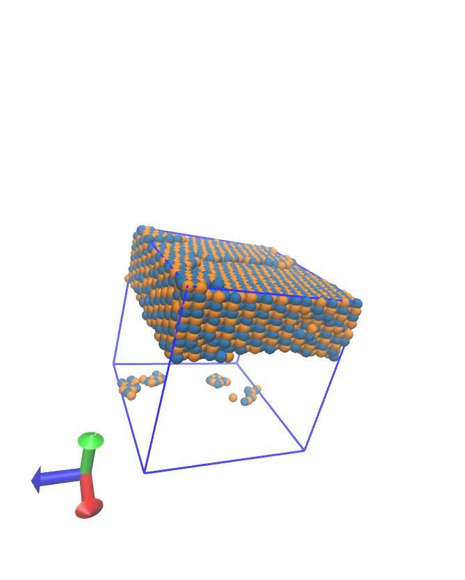
(a) $\rho=0.05$

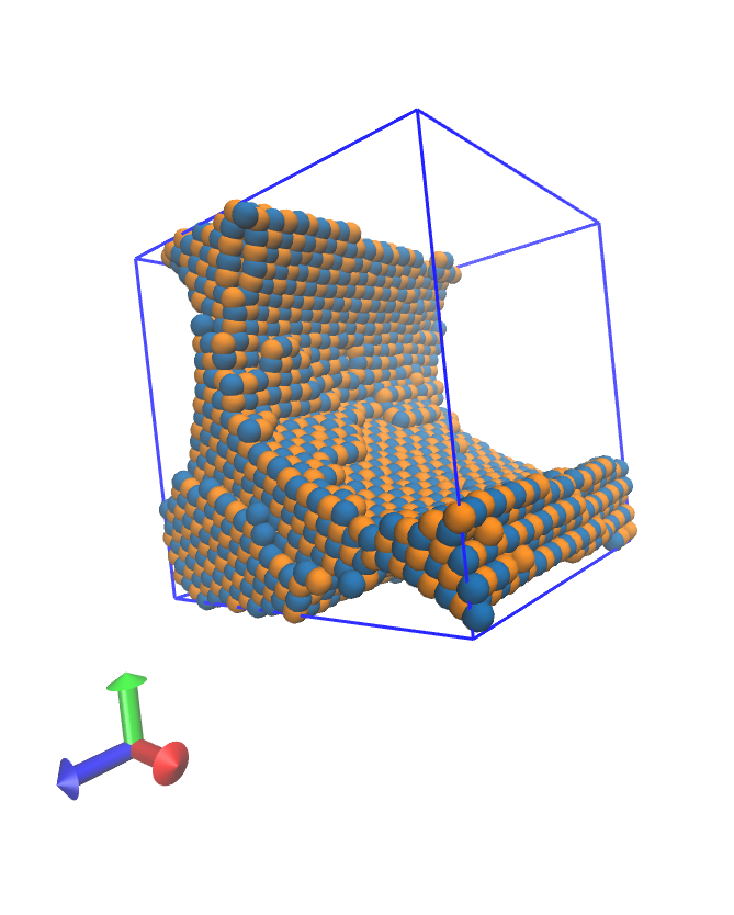
(b) $\rho=0.06$

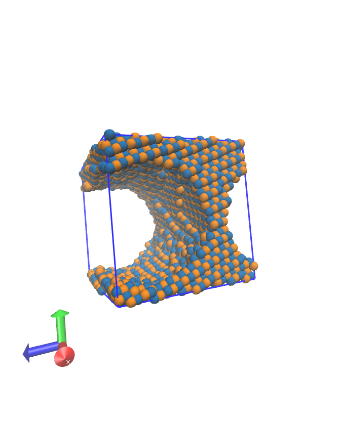
(c) $\rho=0.07$

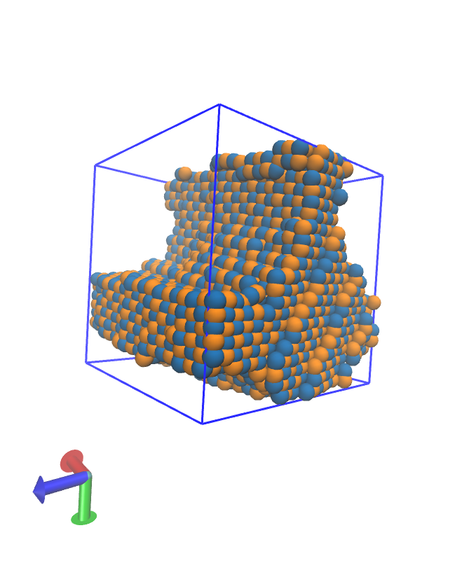
(d) $\rho=0.085$

Figure 1: (Color online) Pasta structures for nuclear matter systems with 6000 nucleons, $x=0.5$ at $T=0.2\,$MeV and densities $\rho$=0.05, 0.06, 0.07 and 0.085 fm^-3. Protons are represented in light color (orange), while neutrons are represented in darker color (blue). The red arrow (out of the page) corresponds to the $x$ coordinate, the green arrow (vertical) to the $y$ coordinate and the blue one (horizontal) to the $z$ coordinate.

We study the properties of a system of 6000 particles (with periodic boundary conditions) using the LAMMPS code lammps with the Pandharipande and screened Coulomb potentials. The total number of particles is divided into protons (P) and neutrons (N) according to values of $x=P/(N+P)=$ 0.3, 0.4 and 0.5. The nuclear system is cooled down from a relatively high temperature ($T\geq 4.0\,$MeV) to a desired cool temperature in small temperature steps ($\Delta T=0.01\,$MeV) with the Nosé Hoover thermostat nose , and assuring that the energy, temperature, and their fluctuations are stable.

Figure 2 shows an example of the energy per nucleon versus the density for systems with 2000 particles at $x=0.5$ and $T=1.5$, $1.0$ and $0.5\,$MeV. Clearly visible are the homogeneous phase (i.e. those under the “$\cup$” part of the energy-density curve), and the loss of homogeneity at lower densities.

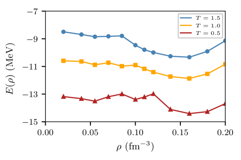
Figure 2: Energy per nucleon versus density for nuclear matter with $x=0.5$ at $T=1.5$ (circles), $1.0$ (squares) and $0.5$ MeV (triangles). The total number of nucleons in the simulating cell was $N=2000$. The system was cooled from 2 MeV to 0.5 MeV.

From Fig. 1 and Fig. 2 it is possible to distinguish three distinct regions to be analyzed. The first one, that goes from very low densities up to approximately $0.08\,$fm^-3 in which the system displays pasta structures, a crystal-like region at densities above approximately $0.14\,$fm^-3, and a transition region between these two dor12A .

II.1.1 Comparison to neutron star matter

Although the present article focuses solely on nuclear matter, it is convenient to compare to neutron star matter, which includes a neutralizing electron gas embedding the nuclear matter. The electron gas is included through a screened Coulomb potential between protons (additional to the Pandharipande potentials) of the Thomas-Fermi form Horo2004 ; Maruyama ; dor12

$$V_{tf}=\displaystyle\frac{q^{2}}{r}e^{-r/\lambda}.$$ (2)

A screening length of $\lambda=20\,$fm is long enough to reproduce the density fluctuations of this model dor14 , likewise the cutoff distance for $V_{tf}$ of 20 fm. Figure 3 shows an example of the pasta structures for symmetric neutron star matter at $T=0.2$ MeV and densities $\rho$=0.05, 0.06, 0.07 and 0.085 fm^-3, respectively. A complete study of phase transitions and the symmetry energy in asymmetric neutron star crusts will presented in the near future.

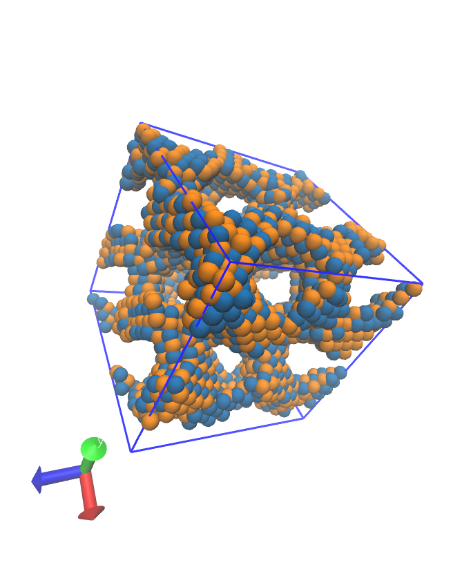
(a) $\rho=0.05$

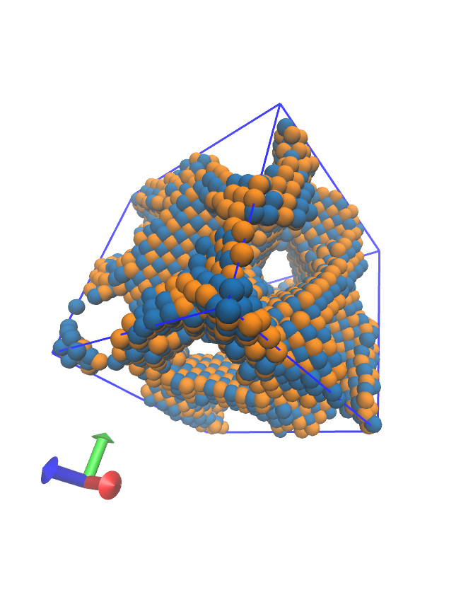
(b) $\rho=0.06$

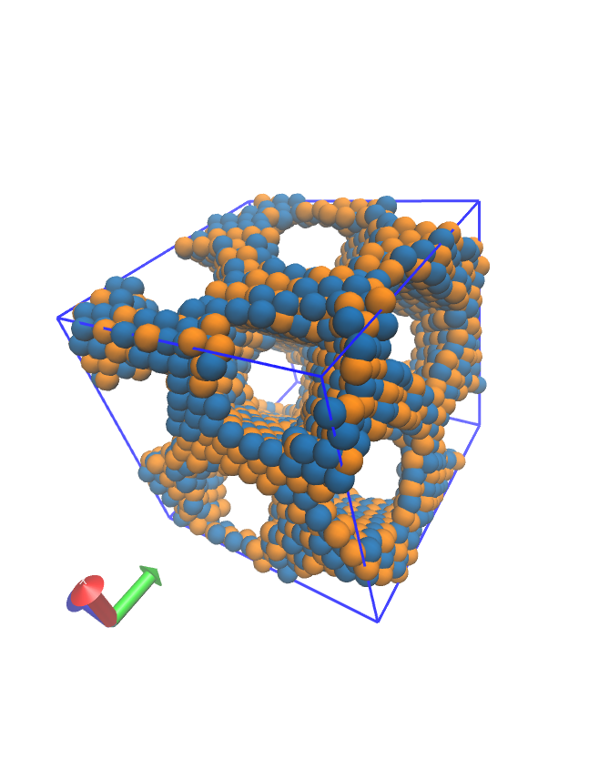
(c) $\rho=0.07$

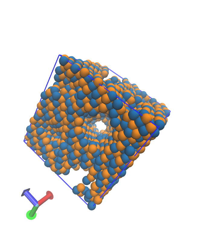
(d) $\rho=0.085$

Figure 3: (Color online) Pasta structures for neutron star matter (with screened Coulomb potential) systems with 4000 nucleons, $x=0.5$ at $T=0.2\,$MeV and densities $\rho$=0.05, 0.06, 0.07 and 0.085 fm^-3. Protons are represented in orange, while neutrons are represented in blue. The red arrow corresponds to the $x$ coordinate, the green arrow to the $y$ coordinate and the blue one to the $z$ coordinate.

II.2 Characterization of the pasta regime

To characterize the pasta, its phase changes and to calculate the symmetry energy we use the the caloric curve, the radial distribution function, the Lindemann coefficient, Kolmogorov statistic, Minkowski functionals and a numerical fitting procedure to estimate $E_{sym}$. These techniques are briefly reviewed next.

II.2.1 Caloric Curve

The heat capacity is a measure of the energy (heat) needed to increase the temperature of the nuclear system, and the plot of energy versus temperature is known as the caloric curve. The energy added to a system is usually distributed among the degrees of freedom of all the particles and, at some precise circumstances, such energy can be used to break inter-particle bonds and make the system go from, say, a solid to a liquid phase; during phase changes an increase of the energy does not result in an increase of the temperature. Likewise, as in different phases there are different number of degrees of freedom, the rate of heating (slope of the caloric curve) is different in the different phases; changes of slope are thus indicators of phase transitions.

II.2.2 Radial distribution function

The radial distribution function is the ratio of the local density of nucleons to the average one, $g(r)=\rho(r)/\rho_{0}$, and it effectively describes the average radial distribution of nucleons around each other. The computation of $g(r)$ is as follows

$$g(r)=\displaystyle\frac{V}{4\pi r^{2}N^{2}}\bigg{\langle}\displaystyle\sum_{i,j}\delta(r-r_{ij})\bigg{\rangle}$$ (3)

where $r_{ij}=|\mathbf{r}_{j}-\mathbf{r}_{i}|$ is the inter-nucleon distance, while $V$ and $N$ are the simulation cell volume and the total number of nucleons, respectively. Thus, $g(r)$ is obtained by tallying the distance between neighboring nucleons at a given mean density and temperature, averaged over a large number of particles. A rigorous definition of $g(r)$ for non-homogeneous systems, such as the pasta, can be found in Appendix A.

The strength of the peaks of $g(r)$ help to detect whether nucleons are in a regular (solid) phase or in a disordered (liquid) system. See Section III for details.

II.2.3 Lindemann coefficient

The Lindemann coefficient lindemann provides an estimation of the root mean square displacement of the particles respect to their equilibrium position in a crystal state, and it serves as an indicator of the phase where the particles are in, as well as of transitions from one phase to another. Formally,

$$\Delta_{L}=\displaystyle\frac{1}{a}\displaystyle\sqrt{\displaystyle\sum_{i=1}^{N}\bigg{\langle}\displaystyle\frac{\Delta r^{2}_{i}}{N}\bigg{\rangle}}$$ (4)

where $\Delta r^{2}_{i}=(r_{i}-\langle r_{i}\rangle)^{2}$, $N$ is the number of particles, and $a$ is the crystal lattice constant; for the nuclear case we use the volume per particle to set the length scale through $a=(V/N)^{1/3}$.

II.2.4 Kolmogorov statistic

The Kolmogorov statistic measures the difference between a sampled (cumulative) distribution $F_{n}$ and a theoretical distribution $F$. The statistic, as defined by Kolmogorov birnbaum , applies to univariate distributions (1D) as follows

$$D_{N}=\mathrm{sup}_{\{x\}}|F_{n}(x)-F(x)|$$ (5)

where “sup” means the supremum value of the argument along the $x$ domain, and $N$ is the total number of samples. This definition is proven to represent univocally the greatest absolute discrepancy between both distributions.

An extension of the Kolmogorov statistic to multivariate distributions, however, is not straight forward and researchers moved in different directions for introducing an achievable statistic gosset . The Franceschini’s version seems to be “well-behaved enough” to ensure that the computed supremum varies in the same way as the “true” supremum. It also appears to be sufficiently distribution-free for practical purposes franceschini .

The three dimensional (3D) Franceschini’s extension of the Kolmogorov statistic computes the supremum for the octants

$$(x<X_{i},y<Y_{i},z < Z_{i}),$$

$$(x<X_{i},y < Y_{i},z>Z_{i}),$$

$$...\ (x > X_{i},y>Y_{i},z>Z_{i})$$ (6)

for any sample $(X_{i},Y_{i},Z_{i})$, $i$ denoting each of the $N$ particles, and chooses the supremum from this set of eight values. The method assumes that the variables $X_{i}$, $Y_{i}$ and $Z_{i}$ are not highly correlated.

In the nuclear case, the Kolmogorov 3D (that is, the Franceschini’s version) quantifies the discrepancy in the nucleons positions compared to the homogeneous case.

It is worth mentioning that the reliability of the 3D Kolmogorov statistic has been questioned in recent years babu . The arguments, however, focus on the correct confidence intervals when applying the 3D Kolmogorov statistic to the null-hypothesis tests. Our investigation does not require computing these intervals, and thus, the questionings are irrelevant to the matter.

II.2.5 Minkowski functionals

Minkowski functionals michielsen are functions designed to measure the size, shape and connectivity of spatial structures formed by the nucleons. For three dimensional bodies these functions are the volume, surface area, Euler characteristic ($\chi$), and integral mean curvature (B). The Euler characteristic can be interpreted as

$$\chi=\mathrm{isolated\ regions}+\mathrm{cavities}-\mathrm{tunnels}$$ (7)

while $B$ is a measure of the curvature of the surface of a given structure. In Ref. dor12A it was found that the pasta structures can be classified according to Table 2.

	B $<$ 0	B $\sim$ 0	B $>$ 0
$\chi>0$	anti-gnocchi		Gnocchi
$\chi\sim 0$	anti-gpaghetti	lasagna	spaghetti
$\chi<0$	anti-jungle gym		jungle gym

Table 2: Integral mean curvature and Euler characteristic values for pasta shapes. The “anti” prefix means the inverted situation between occupied and empty regions. The “jungle gym” stands for a 3D rectangular trellis.

II.2.6 Symmetry energy

The evaluation of the symmetry energy follows the procedure introduced before lopez2014 ; lopez2017 . The symmetry energy is defined as

$$E_{sym}(\rho,T)=\displaystyle\frac{1}{2!}\,\displaystyle\frac{\partial^{2}E(\rho,T,\alpha)}{\partial\alpha^{2}}\bigg{|}_{\alpha=0}$$ (8)

with $\alpha=(N-Z)/(N+Z)=1-2x$. Using the CMD results of the internal energy $E(\rho,T,x)$ it is possible to construct a continuous function by fitting the values of $E(T,\rho,\alpha)$ for each $T$ and $x$ with an expression of the type

$$E(T,\rho,\alpha)=\displaystyle\sum_{i=0}^{3}E_{i}(T,\alpha)\,\rho^{i}$$ (9)

The $\alpha$ dependence of the coefficients $E_{i}(T,\alpha)$ can be extracted from the CMD data calculated at various values of $\alpha$, and assuming an $\alpha$ dependence of the type

$$E_{i}(T,\alpha)=E_{i0}(T)+E_{i2}(T)\,\alpha^{2}+E_{i4}(T)\,\alpha^{4}$$ (10)

with odd terms in $\alpha$ not included to respect the isospin symmetry of the strong force. The symmetry energy is then given by

$$E_{sym}(T,\rho) = E_{02}(T)+E_{12}(T)\rho+$$ (11)

$$+ E_{22}(T)\rho^{2}+E_{32}(T)\rho^{3}$$

with the coefficients $E_{ij}(T)$ obtained from the fit of the CMD data. In our case we calculate the symmetry energy separately for the homogeneous and non-homogeneous cases.

Next, the tools presented in this Section will be used to analyze the pasta structures, determine whether the phase transitions obtained in Ref. dorso2014 for symmetric nuclear matter survive in asymmetric nuclear matter, and what is the behavior of the symmetry energy within the pasta.

II.3 Molecular dynamics simulation of nuclear matter

In what follows, to study infinite systems of isospin-asymmetric nuclear matter, the LAMMPS CMD code was fitted with the Pandharipande potentials and used to track the evolution of systems with $A=$ 4000 or 6000 nucleons situated in a cubic cell under periodic boundary conditions. The isospin content varied from $x=0.3$, $0.4$, and $0.5$, and densities between $0.05\,$fm^-3 to $0.085\,$fm^-3. The temperature was controlled with a Nosé-Hoover thermostat slowly varying from $T$ = 4 MeV down to 0.2 MeV ($\Delta T<0.1\%$). After placing the nucleons at random, but with a minimum inter-particle distance of 0.01 fm, the nucleons were endowed with velocities according to a Maxwell-Boltzmann distribution to correspond to a desired temperature, and the equations of motion were solved to mimic the evolution of the system. The nucleon positions, momenta, energy per nucleon, pressure, temperature, and density, were stored at fixed time-steps.

III Results for nuclear pasta

III.1 Thermodynamic magnitudes

As a first step, we computed the caloric curve for three different proton ratios. Figure 4 shows the response at $\rho=0.05\,$fm^-3 for systems of 6000 nucleons at proton ratios of $x=$0.3, 0.4 and 0.5. The sharp change close to $T=0.5\,$MeV in symmetric nuclear matter was already examined in Ref. dorso2014 . Figure 5 shows an example of the behavior of the Lindemann coefficient as a function of the temperature, compared to the caloric curve for $\rho=0.05\,$fm^-3. This change is a signal of a solid-liquid phase transition within the pasta regime, as concluded in Ref. dorso2014 .

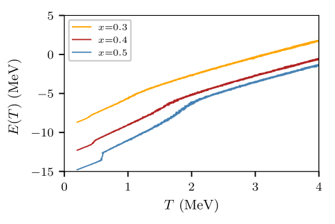
Figure 4: The caloric curve for nuclear matter at $\rho=0.05\,\mathrm{fm}^{-3}$ and $x=0.3$, $0.4$, $0.5$, respectively. The nucleons density was $\rho=0.05\,$fm^-3. The total number of nucleons was 6000.

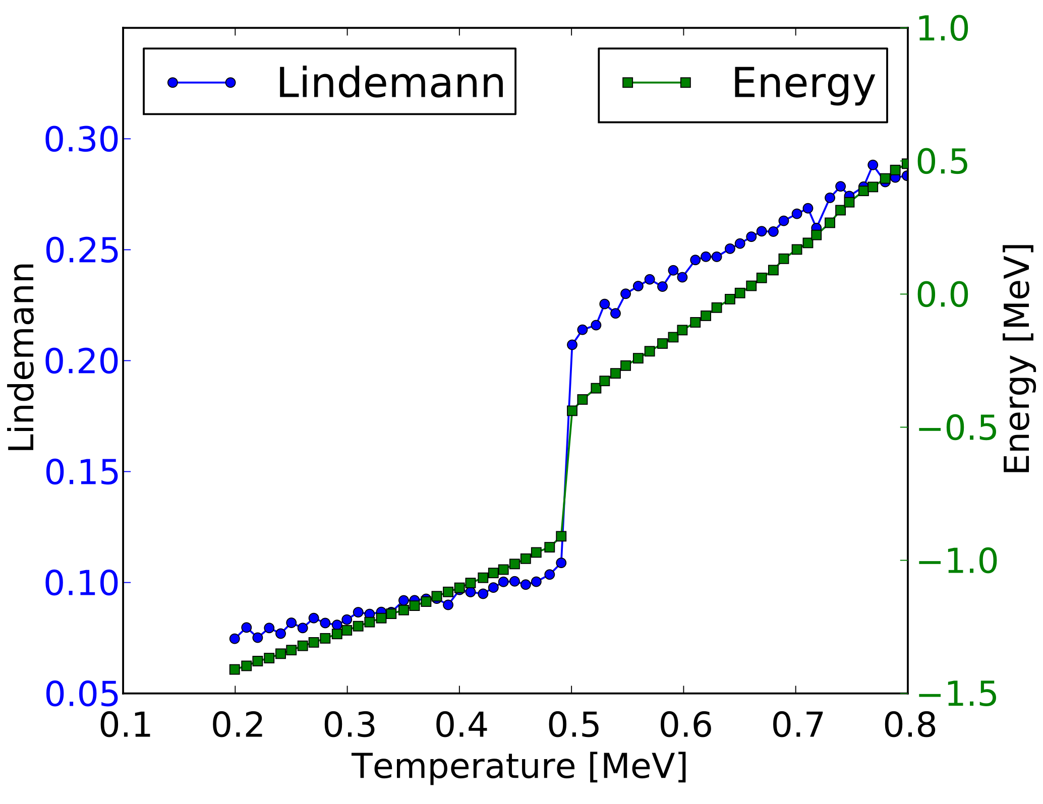
Figure 5: Lindemann coefficient superimposed on the caloric curve for $\rho=0.05\,$fm^-3 for a symmetric system. The sudden change in going from $T<$ 0.5 MeV to $T>$ 0.5 MeV signals a phase change from solid pasta to liquid pasta. Extracted from Ref. dorso2014

.

Figure 4 exhibits, however, a wider picture of the caloric responses. The slope of the curves change gently at “warm” temperatures (say, near $2\,$MeV) attaining lower energies than expected from the extrapolated values for $T>2\,$MeV. It seems, though, that this change in the slope is more significant as $\alpha\rightarrow 0$ ($x\rightarrow 0.5$).

The system pressure also experiences a change in the slope at similar temperatures as the energy, as can be seen in Fig. 6. Notice that the pressure of the symmetric nuclear matter ($x=0.5$) also changes sign, while the pressure of the asymmetric nuclear matter ($x<0.5$) remains positive until very low temperatures. It is clear that the former enters into the metastable regime, while the latter does not completely fulfill this condition.

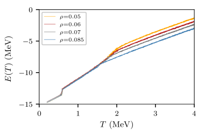
(a) $x=0.5$

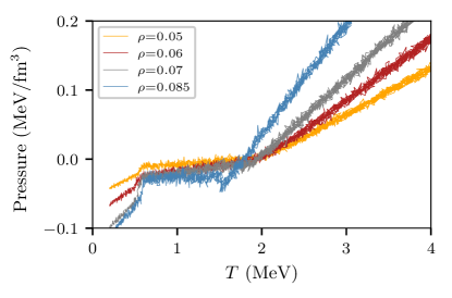
(b) $x=0.5$

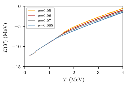
(c) $x=0.4$

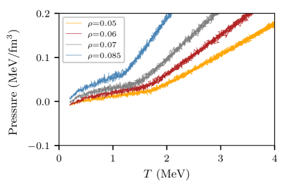
(d) $x=0.4$

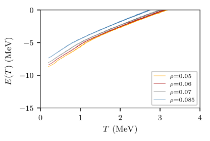
(e) $x=0.3$

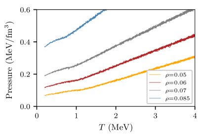
(f) $x=0.3$

Figure 6: (Color online) Energy and pressure as a function of temperature for nuclear matter systems with 6000 nucleons at densities $\rho$=0.05, 0.06, 0.07 and 0.085 fm^-3. Cases (a) and (b) are for symmetric nuclear matter ($x=0.5$) and correspond to the configurations shown in Fig. 1, (c) and (d) are for non-symmetric nuclear matter with $x=0.4$, and (e) and (f) for $x=0.3$.

The change in the pressure sign is meaningful. Positive pressures may be associated to net repulsive inter-particle forces (regardless of momentum), while negative pressures may be associated to net attractive forces. The visual image of a net attractive metastable scenario corresponds to the pasta formation. The fact that pressure does not change sign for asymmetric nuclear matter suggests a more complex scenario; Section III.2 examines the low density regime in detail.

III.2 Microscopic magnitudes

We next explored the radial distribution function $g(r)$ (see Section II.2.2). Figure 7 shows the $g(r)$ for nuclear matter at $\rho=0.085\,$fm^-3 and at three different temperatures (see caption for details). Panel (a) show the results for the symmetric ($x=0.5$) case, and (b) the non-symmetric ($x=0.4$) case.

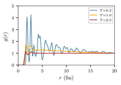
(a) $x=0.5$

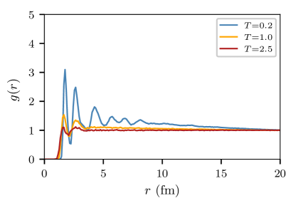
(b) $x=0.4$

Figure 7: (Color online) Radial distribution function $g(r)$ for the case of 6000 nucleons of symmetric (a) and non-symmetric (b) nuclear matter, at $\rho=0.085\,$fm^-3 and $T=0.2\,$MeV, $1.0\,$MeV and 2.5 MeV. The binning is $0.1\,$fm in width in a simulation cell of 41.2 fm of width.

From a very first inspection of Fig. 7 it is clear that the $T=0.2\,$MeV situation corresponds to a solid-like pattern. The local maxima indicate the (mean) equilibrium distance between nucleons in a orderly scheme. The first two maxima near the origin appear sharply, meaning well-arranged neighbors around each nucleon. These maxima are still present at $T=1\,$MeV and $T=2.5\,$MeV, although not as sharp as in the solid-like situation. Thus, the very short range $r<5\,$fm seems not to present an unusual behavior, regardless of the first order transition (solid-to-liquid like) detailed in Section III.1, indicating that in spite of the phase change the pasta structure is maintained.

A noticeable different pattern can be seen in Fig. 7a between the $T=1\,$MeV (metastable) and the $T=2.5\,$MeV (stable) scenario for the range $r>5\,$fm. The metastable scenario exhibits a negative smooth slope, while the stable one displays a vanishing slope. This is in agreement with the pasta formation, as follows.

The $g(r)$ computation involves tallying distances between neighboring nucleons at the nucleons positions (see Eq. (3)). Hence, the $g(r)$ widely samples the inner environment of the pasta, at least for short distances. As the sampled distance increases (inside the pasta), the $g(r)$ is not expected to converge to unity but above unity, since the local average density exceeds the global average density $N/V$. That is what we see in Fig. 7a close to $5\,$fm.

The above reasoning remains valid until the neighboring distances surpasses the inner environment of the pasta. As bubbles or tunnels, or other hollow spaces appear, the tally in Eq. (3) converges to the total number of nucleons inside the simulating cell. Consequently, the distribution $g(r)$ diminishes. A precise computation of $g(r)$ for non-homogeneous media can be seen in Appendix A, together with some theoretical support.

Notice from Fig. 7a that the solid-like situation also resembles the pasta formation since the moving average of the $g(r)$ for $T=0.2\,$MeV exhibits a smooth negative slope.

The argument outlined so far does not hypothesize on the pasta shape. It only compares the average density inside the pasta with respect to $N/V$. Thus, it is expected to hold on a variety of pastas. This was verified for different densities, as shown in Fig. 8.

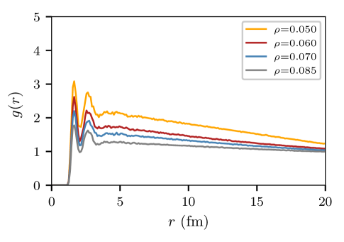
Figure 8: (Color online) Radial distribution function $g(r)$ for the case of 6000 nucleons at $T=1.0\,$MeV and $x=0.5$. The densities are $\rho=0.05$ (top curve), $0.06$, $0.07$ and $0.085\,$fm^-3 (bottom curve). The binning is $0.1\,$fm width, while the simulation cell is approximately 40 fm width.

The non-symmetric case shown in Fig. 7b is somewhat different. The long range $r>5\,$fm appears flattened with respect to the symmetric case (Fig. 7a). Thus, no clear indication of pasta formation can be seen here. The same happened, indeed, with respect to the metastable state in Section III.1. Both, the pressure and the radial distribution seem to fail in order to detect pasta structures.

The visual inspection of the simulation cell shows that pasta structures are actually present in non-symmetric nuclear matter. Figs. 9 and 10 exhibit two non-symmetric situations. Figure 9 actually corresponds to the same configurations as in Fig. 7b but now protons and neutrons are represented separately. The protons actually exhibit a sharp pasta formation (see Fig.  9b). The neutrons’ pattern, instead, appears fuzzy because of the fraction in excess that occupies the empty volume left by the pasta.

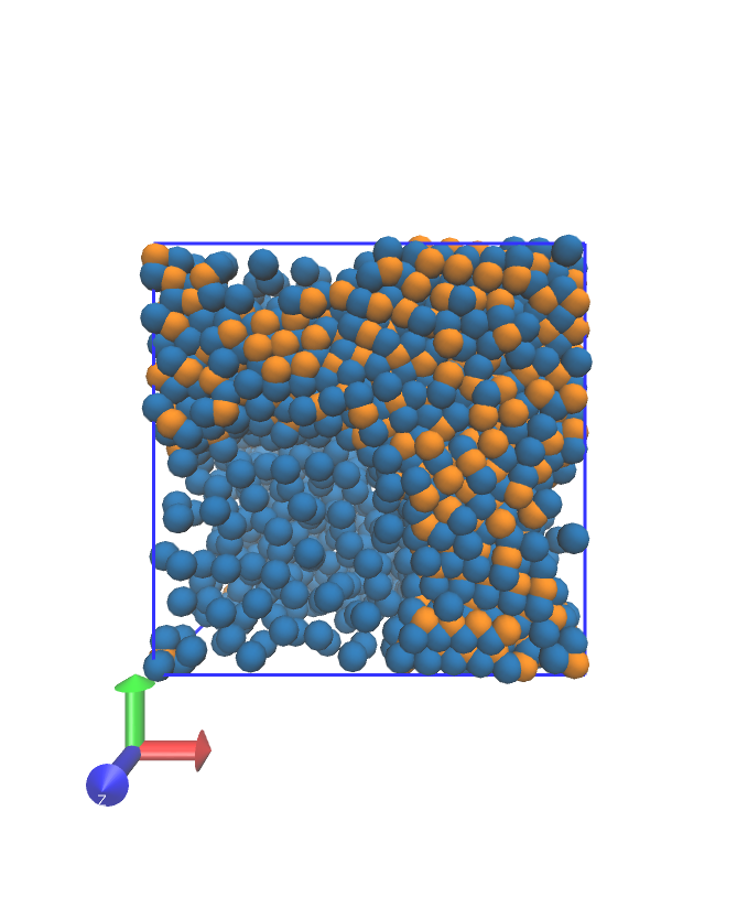
(a)

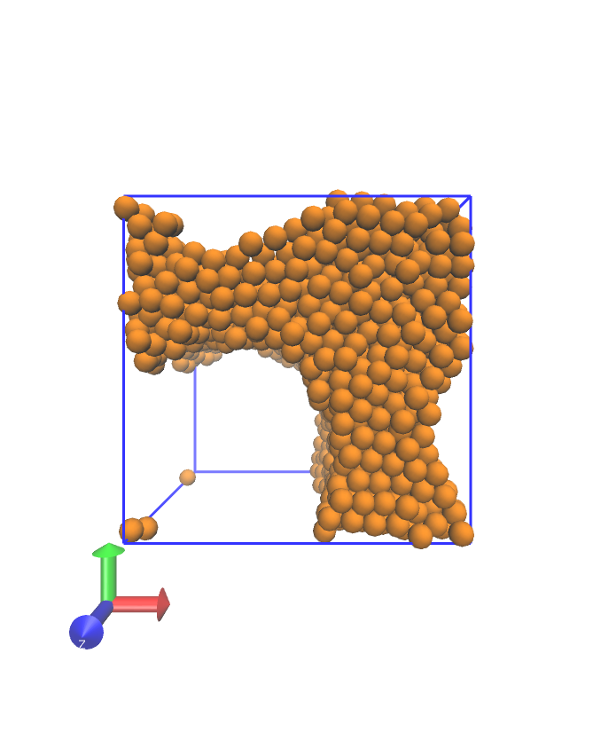
(b)

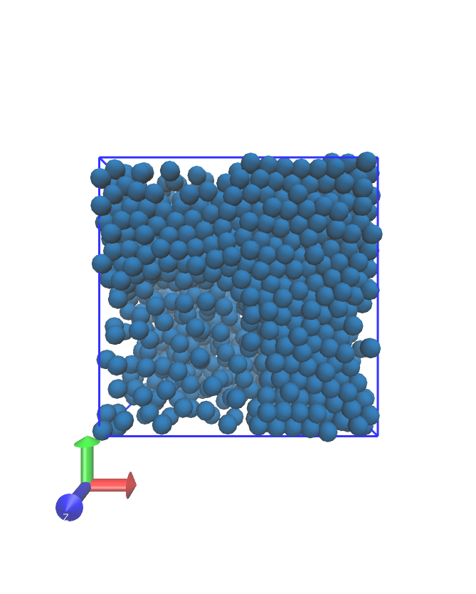
(c)

Figure 9: (Color online) Pasta structures for nuclear matter systems with 6000 nucleons, $x=0.4$ at $T=0.2\,$MeV and density $\rho$=0.085 fm^-3. (a) All nucleons (protons in light color and neutrons in dark), (b) protons only, and (c) neutrons only.

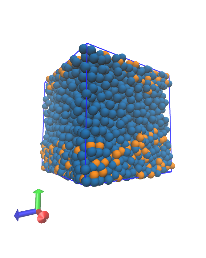
(a)

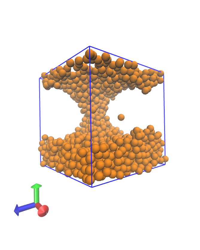
(b)

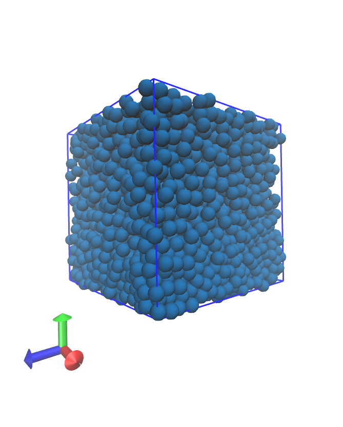
(c)

Figure 10: (Color online) Pasta structures for nuclear matter systems with 6000 nucleons, $x=0.3$ at $T=0.2\,$MeV and density $\rho$=0.085 fm^-3. (a) All nucleons (protons in light color and neutrons in dark), (b) protons only, and (c) neutrons only.

We realize from the above observations that many indicators may fail to recognize the pasta formation in non-symmetric nuclear matter. This is because the neutrons in excess obscure the useful information when mean values are computed. This drawback may also occur in symmetric nuclear matter at the very beginning of the pasta formation (say, at $T\sim 2\,$MeV) since the presence of small bubbles or tiny tunnels may be lost in the averaging process. Section III.3 deals with these issues.

III.3 Morphological indicators

In order to capture the early pasta formation at “warm” temperatures (say, $T\sim 2\,$MeV) we introduce two indicators that do not require computing mean values, namely the Kolmogorov statistic and the Minkowski functionals; the former is not conditioned to space binning, as the latter is, but they both provide different points of view on the pasta formation.

III.3.1 Kolmogorov statistic

The Kolmogorov statistic is known to be “distribution-free” for the univariate distributions case and “almost distribution-free” for multivariate distributions (see Section II.2.4). This section deals with univariate distributions, while the multivariate distributions are left to Section III.4.

The 1D Kolmogorov statistic is useful to study the departure of the nucleons’ position from homogeneity, that is, from the uniform distribution. We applied the statistic separately on each cartesian coordinate, this may be envisaged as the projection of each position on the three canonical axes. Figure 11 shows the corresponding results for an isospin symmetric system at $\rho=0.05\,$fm^-3.

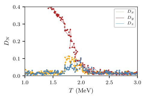
(a)

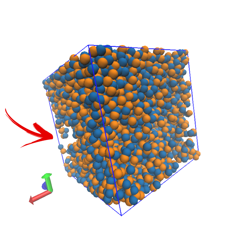
(b)

Figure 11: (Color online) (a) The Kolmogorov 1D statistic vs. temperature. Data corresponds to the position of 6000 nucleons at $\rho=0.05\,\mathrm{fm}^{-3}$ and $x=0.5$ (the same configuration as in Fig. 1a). $D_{x}$, $D_{y}$ and $D_{z}$ correspond to the $x$, $y$ and $z$ Kolmogorov statistics, respectively (see text for details). (b) Visualization of the system analyzed in (a) at $T=2\,$MeV. The arrow points to the most noticeable bubble appearing in the picture.

As can be seen in Fig. 11, the values of the 1D Kolmogorov statistic (i.e. the discrepancy) are negligible for temperatures above $2\,$MeV, as expected for energetic particles moving around homogeneously. At $T\approx 2\,$MeV, the three statistics experience a change in the slope, although $D_{x}$ and $D_{z}$ return to negligible values as the temperature further decreases. The $D_{y}$ statistic, instead, attains a definite departure from homogeneity for $T<2\,$MeV. Recall from Fig. 1a that a lasagna or slab-like structure occurs across the $y$-axis as temperature is lowered.

The 1D Kolmogorov statistic attains the departure from homogeneity at an early stage of the pasta formation. The arrow in Fig. 11b points to the most noticeable bubble appearing in the system at $T=2\,$MeV. The bubble-like heterogeneity also explains the changes in the slope for $D_{x}$ and $D_{z}$ at this temperature, as pictured in Fig. 12. For decreasing temperatures, the bubble widens (on the right side of the image due to the periodic boundary conditions), a tunnel appears (Fig. 12b), and at $T<1.5\,$MeV it finally splits into two pieces while the $(x,y)$ homogeneity gets restored (Fig. 12c) returning $D_{x}$ and $D_{z}$ back to their negligible values.

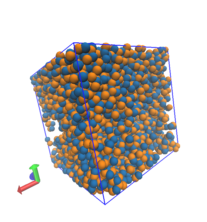
(a) $T=2\,$MeV

(b) $T=1.8\,$MeV

(c) $T=1.5\,$MeV

Figure 12: (Color online) Visualization of 6000 nucleons at $\rho=0.05\,\mathrm{fm}^{-3}$, $x=0.5$ (the same configuration as in Fig. 1a) at three temperatures. (a) A bubble can be seen on the left. (b) A tunnel appears along the $x,y$ plane. (c) The tunnel widens and breaks into two slabs.

We further applied the 1D Kolmogorov statistic on protons and neutrons separately for non-symmetric nuclear matter systems. Figure 13 exhibits the most significant 1D statistics for the densities $\rho=0.05\,\mathrm{fm}^{-3}$ and $\rho=0.085\,\mathrm{fm}^{-3}$, respectively. The corresponding spatial configurations can be seen in Figs. 9 and 10 for $\rho=0.085\,\mathrm{fm}^{-3}$, and in Figs. 14 and 15 for $\rho=0.05\,\mathrm{fm}^{-3}$.

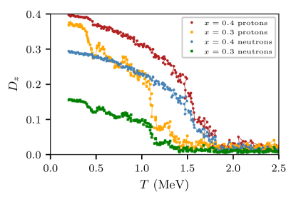
(a) $\rho=0.05\,\mathrm{fm}^{-3}$

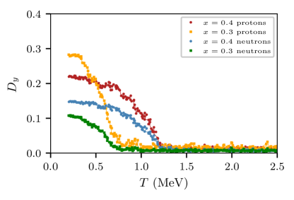
(b) $\rho=0.085\,\mathrm{fm}^{-3}$

Figure 13: (Color online) (a) The Kolmogorov 1D statistic vs. temperature. Data corresponds to the position of 6000 nucleons (no screened Coulomb potential) for $x=0.3$ and $0.4$. (a) The $D_{z}$ statistic ($\rho=0.05\,\mathrm{fm}^{-3}$). (b) The $D_{y}$ statistic ($\rho=0.085\,\mathrm{fm}^{-3}$).

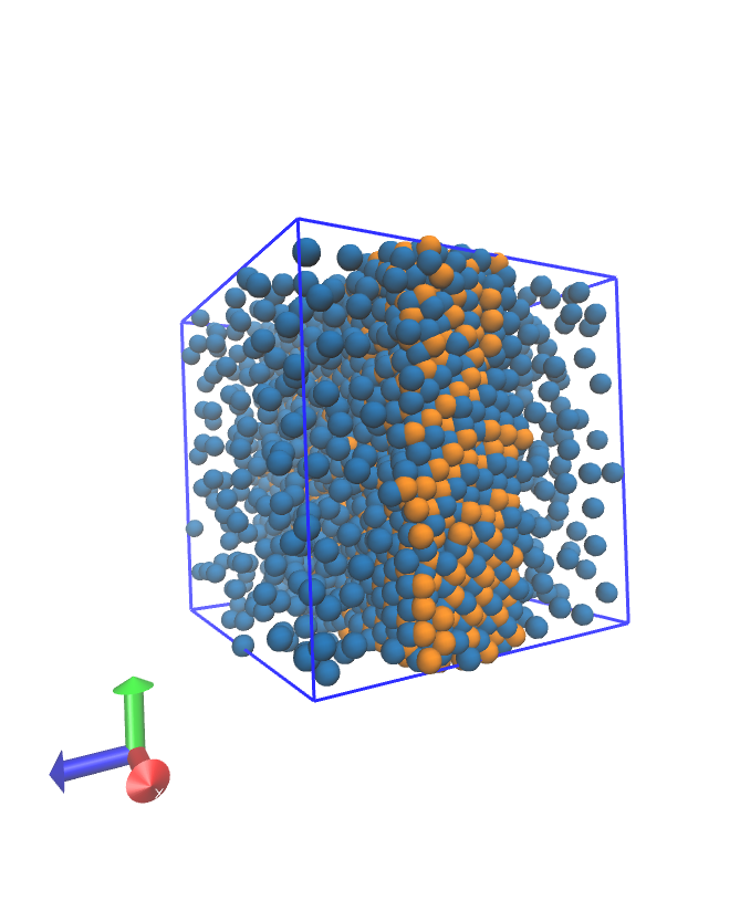
(a)

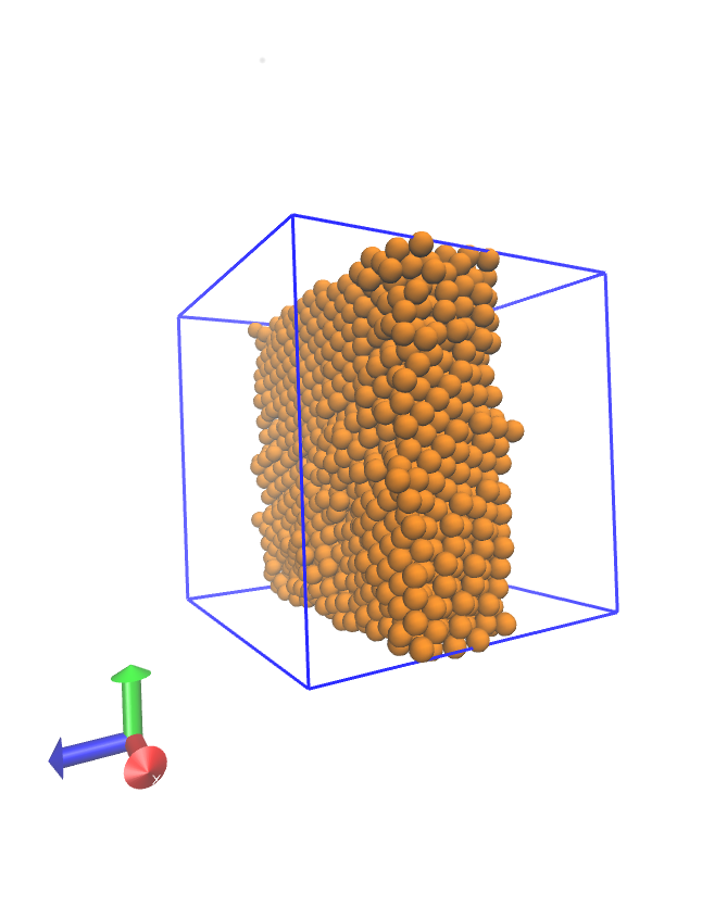
(b)

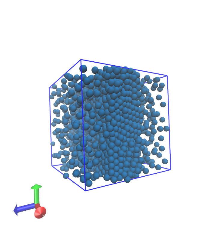
(c)

Figure 14: (Color online) Pasta structures for nuclear matter systems with 6000 nucleons, $x=0.4$ at $T=0.2\,$MeV and density $\rho$=0.05 fm^-3. (a) All nucleons (protons in orange and neutrons in blue). (b) Protons only. (c) Neutrons only.

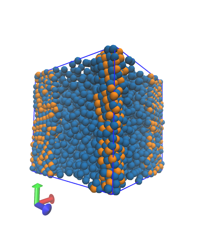
(a)

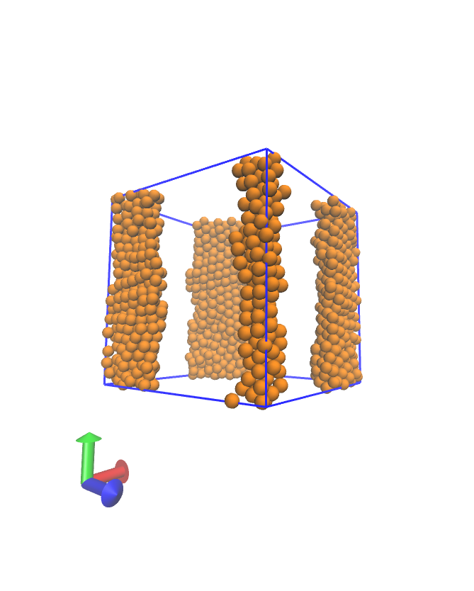
(b)

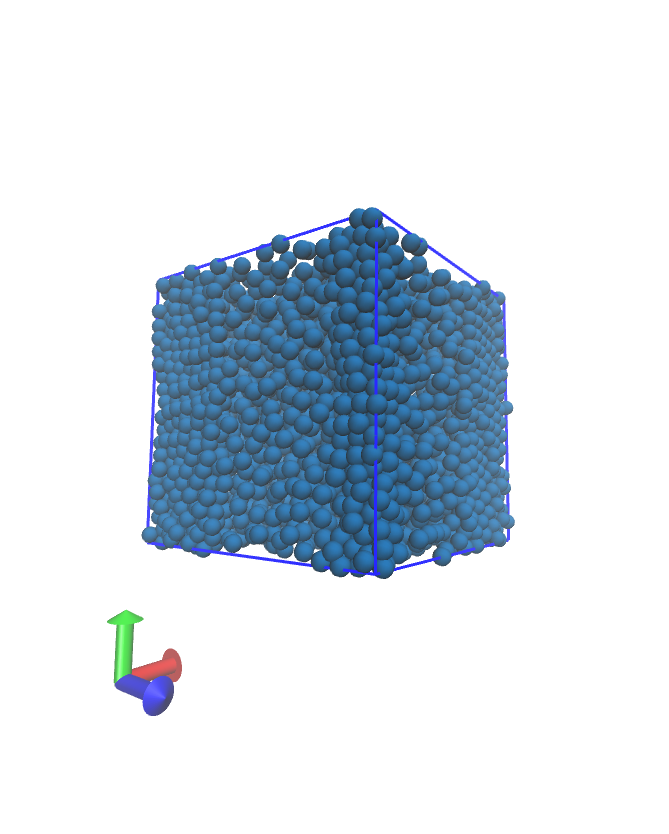
(c)

Figure 15: (Color online) Pasta structures for nuclear matter systems with 6000 nucleons, $x=0.3$ at $T=0.2\,$MeV and density $\rho$=0.05 fm^-3. (a) All nucleons (protons in orange and neutrons in blue). (b) Protons only. (c) Neutrons only.

According to Fig. 13, the temperature threshold at which the 1D Kolmogorov statistic becomes significant, decreases with smaller proton ratios (and fixed density). This is in agreement with the caloric curves presented in Section III.1, but more sharply exposed now. However, both species, protons and neutrons, seem to depart from homogeneity at the same temperature threshold (see Fig. 13). The departure appears more sharply for the protons than for the neutrons. Indeed, the protons attain higher maximum values of $D$ than the neutrons at low temperatures (for the same configuration). The visual inspection of Figs. 9, 10, 14 and 15 confirms this point.

We conclude that the non-symmetric systems do not develop noticeable bubbles or heterogeneities at the same temperature as the symmetric systems do. The excess of neutrons appears to frustrate the pasta formation for a while, but the protons manage to form pasta structures at lower temperatures. The released neutrons get distributed along the cell disrupting the pasta structure, as mentioned in Section III.2.

III.3.2 Minkowski functionals

The Minkowski functionals supply complementary information on the pasta structure from the early stage to the solid-like stage. The accuracy of this information is, however, conditional to the correct binning of the simulation cell. Tiny “voxels” (that is, a high density binning) may produce fake empty voids (artificial bubbles or tunnels) and, on the contrary, oversized voxels may yield a wrong structure of the system due to the lack of details. Therefore, some effort needs to be spent to determine the correct size for the voxels; Appendix B summarizes this procedure.

The simulation cell was first divided into cubic voxels of edge length $d=2.35\,$fm. The Euler functional $\chi$ was computed for symmetric nuclear matter, according to Eq. (7) and the results are shown in Fig. 16. As seen in this figure, the Euler functional $\chi$ for symmetric matter shows three distinct regions as a function of temperature, one at $T>2\,$MeV, one at $T<0.5\,$MeV, and a transition one between these two.

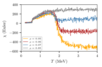
Figure 16: (Color online) The Euler functional $\chi$ as a function of temperature for the densities $\rho=0.05$, $0.06$, $0.07$, $0.085\,$fm^-3 and the proton ratio $x=0.5$. The voxel edge length is $d=2.35\,$fm. The total number of nucleons is $6000$.

At $T>2\,$MeV $\chi$ does not experience significant changes although it attains different values depending on the density. At the low densities of $\rho=0.05\,$fm^-3 and $\rho=0.06\,$fm^-3 $\chi$ exhibits negative values which, according to Eq. (7), indicate that the nucleons are sparse enough to form tunnels and empty regions across the cell. At higher densities, however, $\chi$ becomes positive indicating that tunnels begin to fill forming cavities and isolated regions. This is confirmed by Fig. 17 which shows an inside view of the discretized nuclear matter at $T=2.5\,$MeV, $x=0.5$ and for the four densities under consideration.

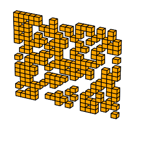
(a) $\rho=0.05$

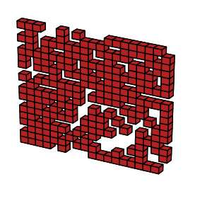
(b) $\rho=0.06$

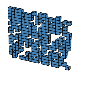
(c) $\rho=0.07$

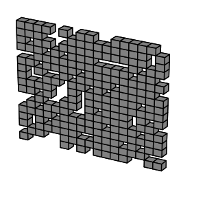
(d) $\rho=0.085$

Figure 17: (Color online) Inside view of discretized nuclear matter with 6000 nucleons at $T=2.5\,$MeV and $x=0.5$. The discretization turned the 6000 nucleons into (approximately) 4300 voxels (edge length $d=2.35\,$fm). Only a slice from the middle ($y$-plane) of the simulation cell is represented. The labels correspond to the density values in fm^-3. The colors are in correspondence with Fig. 16.

The complementarity of $\chi$ over other measures can be seen by comparing it to, for instance, the results of the Kolmogorov statistics (Section III.3.1). As seen in Section III.4, as the nucleons get distributed uniformly at high temperatures neither the 1D nor the 3D Kolmogorov statistic capture the qualitative difference between a tunnel-like and a cavity-like scenarios. Both landscapes may not exhibit noticeable heterogeneities, and thus, they appear to be essentially the same from the point of view of the Kolmogorov statistic.

The energy, however, distinguishes between aforementioned different scenarios. From the comparison between the caloric curves introduced in Section III.1 and the current Euler functional, one can see that both magnitudes are density-dependent in the high temperature regime. While $\chi$ increases for increasing densities, the (mean) energy per nucleon diminishes (see Figs. 6 and 16). Thus, the less energetic configuration (say, $\rho=0.085\,$fm^-3) appears to be a cavity-like (or small bubble-like) scenario from the point of view of $\chi$ (with voxels size of $d=2.35\,$fm).

The Euler functional $\chi$ exhibits a dramatic change at $T\approx 2\,$MeV. This is associated to the departure from homogeneity at the early stage of the pasta formation, as already mentioned in Section III.3.2. Notice that the $\chi$ values for the examined densities join into a single pattern for $T<2\,$MeV, in agreement with the behavior of the energy seen in Fig. 6.

It should be emphasized that although all the examined densities share the same $\chi$ pattern for $T<2\,$MeV, their current morphology may be quite different. Fig. 18 illustrates two such situations (see caption for details). It seems, though, that whatever the morphology, these are constrained to be equally energetic (see Fig. 6).

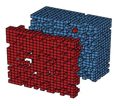
(a) $\rho=0.05$

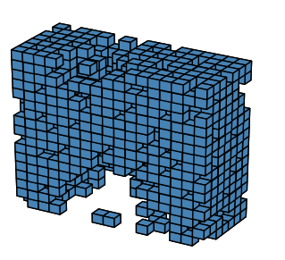
(b) $\rho=0.085$

Figure 18: (Color online) Inside view of discretized nuclear matter with 6000 nucleons at $T=1.5\,$MeV and $x=0.5$. The discretization turned the 6000 nucleons into (approximately) 4300 voxels (edge length $d=2.35\,$fm). (a) Density $\rho=0.05\,$fm^-3. The system split into two major pieces, represented in different colors. Many small pieces in the middle gap can not be seen. (b) Density $\rho=0.085\,$fm^-3. Only a mid-slice of seven voxels thick is shown for practical reasons.

Extending the $\chi$ study for non-symmetric nuclear matter appears to confirm the complexity observed in Sections III.1 and III.3.1. The global pressure does not present negative values for $x=0.4$ and $x=0.3$ at temperatures above the solid-like state. Neither noticeable bubbles nor other heterogeneities could be detected at the early stage of the pasta formation (say, $T\approx 2\,$MeV). We are now able to confirm these results through the $\chi$ functional. Fig. 19 shows the Euler functional for two different densities and $x$= 0.3, 0.4 and 0.5.

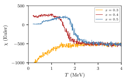
(a) $\rho=0.05$

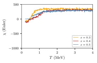
(b) $\rho=0.085$

Figure 19: (Color online) The Euler functional as a function of temperature for $x=0.5$, $0.4$ and $0.3$. The voxel’s edge length is $d=2.35\,$fm. The total number of nucleons is $6000$. (a) $\rho=0.05\,$fm^-3 and (b) $\rho=0.085\,$fm^-3.

Fig. 19a shows three distinct behaviors of $\chi$ at $\rho=0.05\,$fm^-3. The case of symmetric nuclear matter ($x=0.5$) was already analyzed above. The curve for $x=0.4$ appears left-shifted with respect to the symmetric case, in agreement with our previous observation that proton ratios of $x<0.5$ frustrate for a while the pasta formation (see Section III.3.1). In spite of that, the pattern for $x=0.4$ achieves a higher positive value at lower temperatures than the symmetric case indicating that the tunnel-like scenario ($\chi<0$) switched to a bubble-like or an isolated-structure scenario ($\chi>0$). It can be verified from Fig. 20a that this is actually occurring at $T\approx 1\,$MeV; many isolated structures may be visualized in red, while no tunnels seem to be present in the blue region (see caption for details).

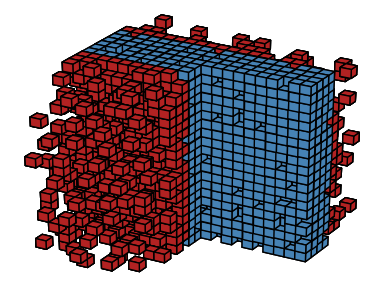
(a) $x=0.4$

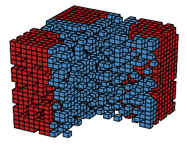
(b) $x=0.3$

Figure 20: (Color online) Inside view of discretized nuclear matter with 6000 nucleons at $T=1.0\,$MeV, and $\rho=0.05\,$fm^-3. A quarter slice has been cut out for a better view of the inner most region of the cell. The discretization turned the 6000 nucleons into (approximately) 3800 voxels (edge length $d=2.35\,$fm). (a) Non-symmetric nuclear matter for $x=0.4$. The red color corresponds to the region mostly occupied by neutrons (compare with Fig. 14). (b) Non-symmetric nuclear matter for $x=0.3$. The blue color corresponds to the region mostly occupied by neutrons (compare with Fig. 15).

The curve of $x=$ 0.3 in Fig. 19a does not change sign nor increases in value at lower temperatures, as opposed to the other two curves. The fact that $\chi<0$ for all of the examined temperatures indicates that tunnel-like landscapes are the relevant ones. Fig. 20b illustrates this scenario: the heavy tunnel-like region (highlighted in blue color) is mostly occupied by neutrons, as shown in Fig. 15, indicating that repulsive forces between neutrons dominate in a large fraction of the cell, and thus producing a positive global pressure all along the examined temperature range, as noticed in Fig. 6. Fig. 19a also show that $\chi$ for $x=0.3$ decreases in magnitude with at lower temperatures; this corresponds to the departure from the spacial homogeneity detected in Fig. 13a, and found by the Kolmogorov statistic and Euler functional to occur at $T\approx 1.5\,$MeV.

At the higher density of $\rho=0.085\,$fm^-3 the behavior of $\chi$ is substantially different. Fig. 19b shows the temperature dependence of $\chi$ for $x=$ 0.3, 0.4 and 0.5; both isospin asymmetric cases are qualitatively similar to the symmetric one. An inspection of the voxels’ configuration (not shown) confirms that tunnels become relevant at very low temperatures; this can be checked from the configurations presented in Figs. 9 and 10.

For obvious reasons the analysis of the $\chi$ functional cannot be applied to protons and neutrons separately, as it was done with the Kolmogorov statistic; excluding either protons or neutrons would produce fake voids, overestimating the total number of tunnels or cavities.

We summarize the results from this section as follows. At $T\approx 2\,$MeV the Euler functional $\chi$ of isospin-symmetric low-density systems ($\rho<0.06\,$fm^-3) show drastic changes from negative to positive values indicating a transition from a void-dominated regime to one with bubbles and isolated regions. Higher density systems ($\rho>0.06\,$fm^-3), in spite of always having $\chi>0$, also increase the value of their $\chi$ at this temperature, reaching a common maximum for all densities at $T\approx 1.5\,$MeV. This maximum corresponds to the formation of bubbles or isolated regions, and indicates the formation of the pasta near the solid-liquid transition; recall that the Kolmogorov statistic was able to detect the pasta formation since the bubbles or isolated regions stage.

For isospin asymmetric systems the low-density ($\rho\approx 0.05\,$fm^-3) growth of $\chi$ is also observed but only for $x=$ 0.4 and 0.5; systems at $x=$ 0.3 have $\chi<0$ at all temperatures. At higher densities ($\rho\approx 0.08\,$fm^-3) the Euler functional is always positive for all temperatures.

Table 2 classifies the pasta according to the sign of $\chi$ and the curvature $B$, and it was a goal of the present study to extend this classification for isospin asymmetric systems, but our results indicate that this labeling becomes meaningless for the non-symmetric case. For a given temperature, the $\chi$ functional attains positive or negative values depending on the isospin content and the density of the system. In general, the excess neutrons obscure the pasta structures for the protons and, thus, the early stage of the pasta formation (that is, the formation of bubbles or isolated regions) is not detectable. In spite of this, we observe that the system departs from homogeneity at $T\sim 1.5\,$MeV (see, for example, Fig. 13a).

III.4 Symmetry energy and nuclear pasta

We now study the symmetry energy of nuclear matter in the pasta region. As stated at the end of Section II.1.1, at a given temperature the energy $E(\rho)$ showed three distinct behaviors as a function of the density: the pasta region for densities below $0.085\,$fm^-3, the crystal-like region for densities above $0.14\,$fm^-3, and an intermediate region in between the first two. In what follows we will focus on the symmetry energy in the pasta region.

Fig. 21 shows the computed symmetry energy as a function of the temperature for the four examined densities. The $E_{sym}$ was computed through the fitting procedure outlined in Section II.2.6. An analysis of the fitting errors can be found in Appendix C.

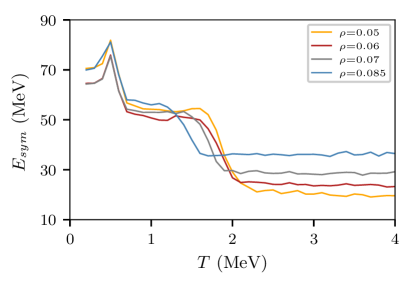
Figure 21: (Color online) Symmetry energy as a function of the temperature for four density values, as indicated in the insert. The system corresponds to nuclear matter with 6000 nucleons.

Several distinct regions can be distinguished for $E_{sym}$ in Fig. 21. In cooling, a liquid system with $T>2\,$MeV starts with a low value of $E_{sym}$. Upon entering the $T<2\,$MeV region and until $T\approx 1.5$ MeV, the symmetry energy increases in magnitude while the liquid pasta is formed. Its value stabilizes in an intermediate value in the warm-to-low temperature range of $0.5$ MeV$<T<1.5$ MeV where the liquid pasta exists. At $T<0.5$ MeV, when the liquid-to-solid phase transition happens within the pasta, the symmetry energy reaches its highest value. We now look at these different stages in turn.

In the higher temperature range, $T>2\,$MeV, the symmetry energy has different magnitudes for the four densities explored (see Fig. 21), with the higher values of $E_{sym}$ corresponding to higher densities. Noticing that this relationship is also maintained by the Euler functional ($\chi$) shown in Fig. 16, it is possible to think that there is a connection between the symmetry energy and the morphology of the system. Remembering from Section III.3.2 that at those temperatures higher densities are associated to cavity-like or isolated regions, and lowest densities with tunnel-like structures, it is safe to think that $E_{sym}$ increases as the tunnels become obstructed and cavities or isolated regions prevail.

Between $1.5$ MeV $<T<2$ MeV the symmetry energy appears to vary in a way resembling the variation of the 3D Kolmogorov statistic, $D$, during the pasta formation stage. To test this hypothesis Fig. 22 compares the variation of $E_{sym}$ with that of $D$ as a function of temperature for the four densities of interest, and finds a good match between both quantities. This interesting observation allows us to use the reasonings in Section III.3.2 to conclude that the variation of $E_{sym}$ can be associated to the changes of the Euler functional $\chi$ (see Fig. 16), which in turn are associated to the morphology of the nuclear matter structure. Indeed one can conclude that as the pasta is formed during cooling, the symmetry energy increases in magnitude.

The value of $E_{sym}$ between $0.5$ MeV $<T<1.5$ MeV corresponds to the pasta structures filled with liquid nuclear matter. Its change at around $T\approx 0.5$ MeV happens at the same temperature at which the caloric curve and the Lindemann coefficient undergoes similar changes (cf. Fig. 5), indicating the phase transition between a liquid pasta ($T>$ 0.5 MeV) and a solid pasta ($T<$ 0.5 MeV). Here one can concluded that the symmetry energy attains its largest value in solid pastas.

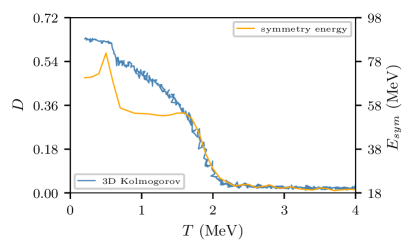
(a) $\rho=0.05$

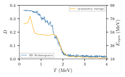
(b) $\rho=0.06$

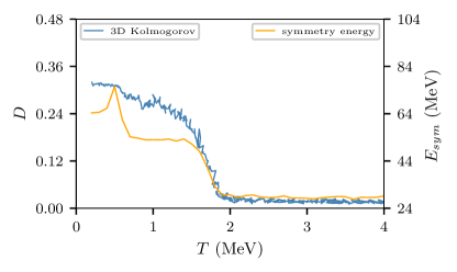
(c) $\rho=0.07$

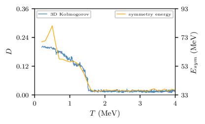
(d) $\rho=0.085$

Figure 22: (Color online) Symmetry energy (right scale) and 3D Kolmogorov statistic (left scale) as a function of the temperature, for nuclear matter with 6000 nucleons at $x=0.5$. The corresponding densities are indicated below each plot (units fm^-3).

Finally, it is worth noting that the values of $E_{sym}$ attained in the studied densities and temperatures are not directly comparable to those calculated in lopez2017 for the liquid-gas coexistence region and compared to experimental results. This lack of comparability comes, first, because the calculation of Fig. 4 in lopez2017 was obtained at higher temperatures ($2$ MeV $<T<5$ MeV) and lower densities ($\rho<$ 0.03 fm^-3), and, second, such calculation was performed with data from a homogeneous medium while the present one uses data from a pasta-structured system. In spite of these differences, it is reassuring that the values of $E_{sym}$ obtained in the present study for the highest temperatures used in the present study, $T>2$ MeV, are within the range of values calculated in lopez2017 for the highest densities considered in such study, namely 0.05 fm${}^{-3}<\rho<$ 0.06 fm^-3.

IV Conclusions

In this article we have investigated the formation of the pasta in nuclear matter (according to the CMD model), its phase transitions and its symmetry energy. In particular we focused in isospin symmetric ($x=0.5$) and isospin asymmetric ($x=0.3$ and 0.4) nuclear matter. We explored, first, if the pasta structures found in symmetric nuclear matter exist in non-symmetric systems and, second, if the solid-to-liquid phase transitions found in Ref. dorso2014 survived in neutron-rich nuclear matter. Lastly, we studied the behavior of the symmetry energy in systems with pasta configurations and whether it is connected to the isospin content, the morphology of the pasta and to the phase transitions.

After introducing a plethora of simulation and computational tools, molecular dynamics simulations were used to produce homogeneous systems that, when cooled down below $T\approx 2$ MeV, were reconfigured into pasta structures; this happened for systems with proton to neutron ratios of $x=0.3$, 0.4 and 0.5, densities in the range of 0.05 fm${}^{-3}\rho<$ 0.08 fm^-3, and were observed by directly drawing the structures, cf. Fig. 1.

Studying the caloric curve (cf. Figs. 4 and 6), and the Lindemann coefficient (cf. Fig. 5) allowed the detection of phase transitions as the nuclear matter system cooled down. The slopes of the caloric curves and of the pressure-temperature curves were also found to vary with density as seen in Fig. 6. A metastable region (i.e. negative pressure) appears to exist only for symmetric systems but not for neutron-rich media.

The radial distribution function allowed the study of the inner structure of the matter filling the pasta structures. Figs. 7 and 8 indicate that at very low temperatures ($T<0.5\,$MeV) the pasta is in a solid state, but at higher temperatures ($0.5\,$ MeV $<T<1.5\,$MeV) it transitions to a liquid phase while maintaining the pasta structure.

Continuing with a study of the departure from homogeneity, the 1D Kolmogorov statistic $D$ was applied separately on each Cartesian coordinate. Figure 11 showed homogeneity in isospin symmetric and non-symmetric systems at temperatures above $2\,$MeV, but at $T\approx 2\,$MeV, $D_{y}$ showed a definite departure from homogeneity for $T<2\,$MeV in agreement with the formation of lasagnas seen in Fig. 1a. Applying the 1D Kolmogorov statistic on protons and neutrons separately shows that in non-symmetric systems the signal from the 1D Kolmogorov statistic appears stronger for protons than for neutrons indicating that in neutron-rich systems the excess neutrons delay the formation of the pasta formation while the protons indeed form pasta structures at lower temperatures.

This complex behavior was corroborated by the Euler functional $\chi$ which showed jumps at the same temperatures at which the phase changed. $\chi$ was found to be correlated, depending on the density, with the existence of tunnels, empty regions, cavities and isolated regions. Indeed, at $T\approx 2\,$MeV in isospin-symmetric low-density systems ($\rho<0.06\,$fm^-3) changes of $\chi$ reflect transitions from a void-dominated to a bubble-dominated region, and at higher densities ($\rho>0.06\,$fm^-3) $\chi$ reaches a maximum when the pasta forms at the solid-liquid transition. Likewise, for isospin asymmetric systems at low-densities ($\rho\approx 0.05\,$fm^-3) $\chi$ attained positive or negative values depending on the isospin content and the density of the system.

All of these phase changes that occur during cooling were reflected in the values of the symmetry energy, which showed different behavior as a function of the temperature (cf. Fig. 21). At the higher temperatures ($T>2\,$MeV), $E_{sym}$ had different magnitudes for each of the four densities studied, indicating that in homogeneous systems the symmetry energy increases with the density. In the transition from homogeneity to a liquid-filled pasta $E_{sym}$ varies in the same way as the 3D Kolmogorov statistic $D$, and the Euler functional $\chi$, showing its dependence on the morphology of the nuclear matter structure. The transition from a liquid pasta ($T>$ 0.5 MeV) to a solid pasta ($T<$ 0.5 MeV) was also reflected on the value of $E_{sym}$ with an increase to its largest value.

In conclusion, classical molecular dynamics simulations show the formation of pastas in isospin symmetric and non-symmetric systems. The computational tools developed and applied, although not perfect, demonstrated their usefulness to detect the in-pasta phase transitions first seen in Ref. dorso2014 , and to extend the calculation of the symmetry energy of Ref. lopez2017 to lower temperatures, and connect its value to the structure and thermodynamics of the neutron-rich pasta.

We acknowledge that, although useful for a first study, the used tools produced a somewhat fuzzy picture of the nucleon dynamics within the pasta, and that these tools need to be refined in the future. In summary the pasta structures were fairly detected at temperatures as high as $T\sim 2\,$MeV, the radial distribution function gave information to infer a phase transition within the pasta, and the Kolmogorov statistic and the Minkowski functional were useful in pointing at the early stage of the pasta formation. Future studies will try to refine these tools and apply them to study the formation of the pasta, possible phase transitions and the role of the symmetry energy in neutron-rich neutron star matter.

Appendix A The radial distribution $g(r)$

A rigorous definition for the radial distribution function $g(r)$ starts from the following distance distribution

$$g(\mathbf{r})=\displaystyle\frac{1}{\rho_{0}}\bigg{\langle}\displaystyle\frac{1}{N}\displaystyle\sum_{i=1}^{N}\displaystyle\sum_{j\neq i}^{N}\delta(\mathbf{r}-\mathbf{r}_{ij})\bigg{\rangle}$$ (12)

where $\rho_{0}=N/V$ is the (mean) density in the simulation cell of volume $V$ (or equivalently $L^{3}$). $\mathbf{r}_{ij}=\mathbf{r}_{j}-\mathbf{r}_{i}$ is the distance vector between the particle $i$ and the particle $j$. The $\delta(\cdot)$ function corresponds to the Dirac delta. The mean value indicated by $\langle\cdot\rangle$ corresponds to the average operation over successive time-steps.

In order to illustrate the pattern of the $g(r)$ due to a pasta structure, we assume that particles form a homogeneous slab (that is, a lasagna-like structure) bounded between the $\pm z_{0}$ (horizontal) planes. The slab is quasi static, meaning that no averaging over successive time-steps is required.

We first consider a small region $\Omega(\mathbf{r})$ with volume $\delta x\,\delta y\,\delta z$ in the $\mathbf{r}$ domain. Thus, we may evaluate the expression (12) as follows

$$\int_{\Omega(\mathbf{r})}g(\mathbf{r})\,d^{3}x=\displaystyle\frac{1}{\rho_{0}}\,\displaystyle\frac{1}{N}\displaystyle\sum_{i=1}^{N}\sum_{j\neq i}^{N}\int_{\Omega(\mathbf{r})}\displaystyle\delta(\mathbf{r}-\mathbf{r}_{ij})\,d^{3}x$$ (13)

where the integral on the right-hand side equals unity at the positions $\mathbf{r}=\mathbf{r}_{ij}$ within $\Omega(\mathbf{r})$.

We now proceed to evaluate the sum over the $j\neq i$ neighbors of the particle $i$. The counting of neighbors is proportional to $\delta x\,\delta y\,\delta z$ since the volume $\Omega(\mathbf{r})$ is very small. Thus, the tally is

$$\sum_{j\neq i}^{N}\int_{\Omega(\mathbf{r})}\displaystyle\delta(\mathbf{r}+\mathbf{r}_{i}-\mathbf{r}_{j})\,d^{3}x\approx\rho(\mathbf{r}+\mathbf{r}_{i})\,\delta x\,\delta y\,\delta z$$ (14)

The magnitude $\rho(\mathbf{r}+\mathbf{r}_{i})$ refers to the density within the small region $\Omega(\mathbf{r}+\mathbf{r}_{i})$, its value remains constant inside the slab and vanishes outside. In fact, $\rho$ can be expressed as $\rho_{s}\,\Theta(z_{0}-|z+z_{i}|)$, with $\Theta(\cdot)$ representing the Heaviside function, and $\rho_{s}$ being the slab density ($\rho_{s}>\rho_{0}$).

The sum over the $i$ particles is evaluated through the integral of the infinitesimal pieces $\rho_{s}\,d^{3}x^{\prime}$. Thus,

$$\sum_{i=1}^{N}\rho(\mathbf{r}+\mathbf{r}_{i})\approx\displaystyle\int_{\mathrm{slab}}\!\!\rho_{s}^{2}\,\Theta(z_{0}-|z+z^{\prime}|)\,d^{3}x^{\prime}$$ (15)

where the slab domain corresponds to the bounded region $|z^{\prime}|\leq z_{0}$. Notice that this integral vanishes for $|z|\geq 2z_{0}$ and equals $\rho_{s}^{2}L^{2}\,(2z_{0}-|z|)$ otherwise. The $g(\mathbf{r})$ function is then

$$g(\mathbf{r})\approx\displaystyle\frac{\rho_{s}}{\rho_{0}}\,\bigg{(}1-\displaystyle\frac{|z|}{2z_{0}}\bigg{)}\ \ \ ,\ \ \ |z|<2z_{0}$$ (16)

assuming that $g(\mathbf{r})$ is somewhat fixed inside the small domain $\Omega(\mathbf{r})$ in (13). We further replaced $N$ by $\rho_{s}\,2z_{0}L^{2}$ in (13).

The expression (16) is not exactly the radial distribution function yet because of the angular dependency of $g(\mathbf{r})$. This dependency may be eliminated by integrating $g(\mathbf{r})$ over a spherical shell of radius $r$, which introduced the normalization factor $4\pi r^{2}$ in agreement with Eq. (3). The expression for the radial distribution then reads

$$g(r)=\displaystyle\frac{1}{4\pi r^{2}}\,\displaystyle\int_{S}\displaystyle\frac{\rho_{s}}{\rho_{0}}\,\bigg{(}1-\displaystyle\frac{r|\cos\theta|}{2z_{0}}\bigg{)}\,r^{2}\sin\theta\,d\theta\,d\varphi$$ (17)

where $z=r\,\cos\theta$. Notice that this expression is valid along the interval $|\cos\theta|<2z_{0}/r$ whenever $2z_{0}<r$, but it is constrained to the natural bound $|\cos\theta|\leq 1$ if $2z_{0}\geq r$. The integration of (17) finally yields

$$g(r)=\left\{\begin{array}[]{lcl}\displaystyle\frac{\rho_{s}}{\rho_{0}}\,\bigg{(}1-\displaystyle\frac{r}{4z_{0}}\bigg{)}&\mathrm{if}&r<2z_{0}\\ &&\\ \displaystyle\frac{\rho_{s}}{\rho_{0}}\,\displaystyle\frac{z_{0}}{r}&\mathrm{if}&r>2z_{0}\\ \end{array}\right.$$ (18)

Notice that as $r\rightarrow 0$, $g(r)$ correctly goes to the limit of $g(r)\rightarrow\rho_{s}/\rho_{0}$. Similarly, for larger values of $r$, and up to $r<2z_{0}$, $g(r)$ decreases linearly, as observed in Fig. 8 for different values of $\rho_{0}$.

Eq. (18) also indicates that $g(2z_{0})\approx 1$ in the case that $\rho_{s}/\rho_{0}\approx 2$, in agreement with Fig. 8 where $g(r)$ tends to unity at $20\,$fm (for simulation cells of $L\sim 45\,$fm); this figure, however, does not show the behavior beyond $20\,$fm as the statistics that can be collected for distances above $L/2$ are very poor.

From literature references, $g(r)$ is supposed to converge to unity as $r\rightarrow\infty$. But, according to (18), the radial distribution vanishes at this limit. The disagreement corresponds to the fact that the condition $g(\infty)=1$ is only valid for homogeneous systems. The expression (18) can actually meet this condition if the slab occupies all the simulation cell, since $\rho_{s}\rightarrow\rho_{0}$ and $z_{0}\rightarrow\infty$ (for periodic boundary conditions).

Appendix B The Minkowski voxels

The Minkowski functionals require the binning of space into “voxels” (that is, tridimensional “pixels”). Each voxel is supposed to include (approximately) a single nucleon. But this is somehow difficult to achieve if the system is not completely homogeneous (and regular).

We start with a simple cubic arrangement of 50% protons and 50% neutrons as shown in Fig. 23. The system is at the saturation density $\rho_{0}=0.16\,$fm^-3 (see caption for details).

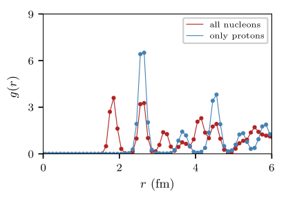
(a)

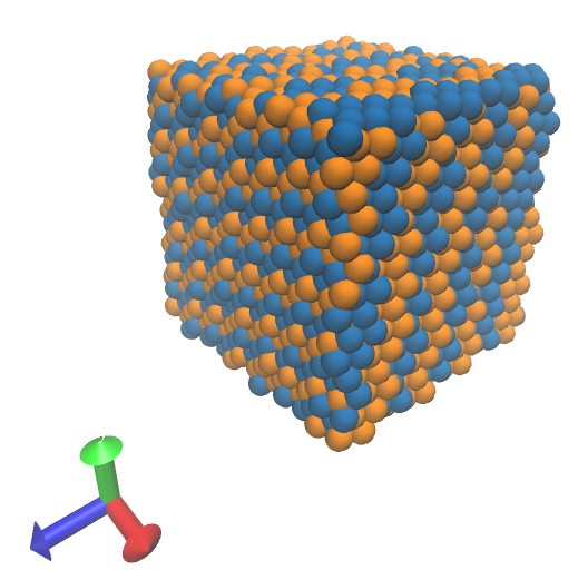
(b)

Figure 23: (Color online) (a) Radial distribution function $g(r)$ for the case of 5832 nucleons ($x=0.5$) at $\rho=0.16\,$fm^-3 and $T=0.1\,$MeV. The binning is $0.05\,$fm. The symbols in blue correspond to the $g(r)$ for protons only. The symbols in red correspond to the $g(r)$ computed over all the nucleons. The first peak for the blue symbols occurs at $2.65\,$fm. The first peak for the red symbols occurs at $1.85\,$fm. (b) A snapshot of the system at $T=0.1\,$MeV.

Notice from Fig. 23 that the nearest distance between protons and neutrons is $1.85\,$fm. Likewise, the nearest distance between nucleons of the same species is approximately $2.65\,$fm (that is, the position of the second peak). It can be verified that the latter is approximately $\sqrt{2}\times 1.85\,$fm, as expected for the simple cubic arrangement (within the $g(r)$ binning errors).

Fig. 24a reproduces the same pattern for the distribution $g(r)$ over all the nucleons. It further shows the Euler functional $\chi$ as a function of the voxel’s width (see caption for details). Both curves share the same abscissa for comparison reasons. For small values of $d$ the functional $\chi$ is negative (not shown), meaning that the voxels are so small that tunnels prevail in the (discretized) system. At $d=1.65\,$fm this functional arrives to a maximum where cavities or isolated regions prevail. Some cavities may be “true” empty regions but other may simply be fake voids. The most probable ones, however, correspond to fake voids since the $g(r)$ pattern actually presents a maximum at $r>1.65\,$fm. Thus, increasing the voxel’s size will most probably cancel the fake cavities.

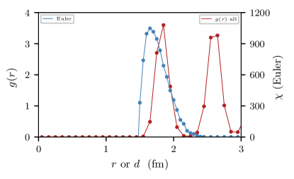
(a)

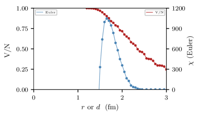
(b)

Figure 24: (Color online) Analysis of the same system as in Fig. 23 (with $N=5832$ nucleons). (a) On the left scale (red symbols), the radial distribution function $g(r)$. On the right scale, the Euler functional $\chi$ as a function of the voxel’s edge length $d$. (b) On the left scale (blue symbols), the first Minkowski functional (volume) as a function of the voxel’s edge length $d$. The volume is normalized by $N$. On the right scale, the same the Euler functional $\chi$ as in (a) for comparison reasons.

The particles located at the first maximum of $g(r)$ (at the saturation density) may be envisaged as touching each other in a regular (simple cubic) array. Therefore, the mean radius for a nucleon should be $1.85/2\,$fm. This means, as a first thought, that binning the space into voxels of width $1.85\,$fm will include a single nucleon per voxels. This is, however, not completely true since approximately half of the first neighbors exceeds the $1.85\,$fm (see first peak in Fig. 23). Many voxels will be empty, and thus, a relevant probability of finding fake voids exists. Fig. 24a illustrates this situation.

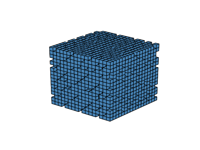
(a) $d=1.85$

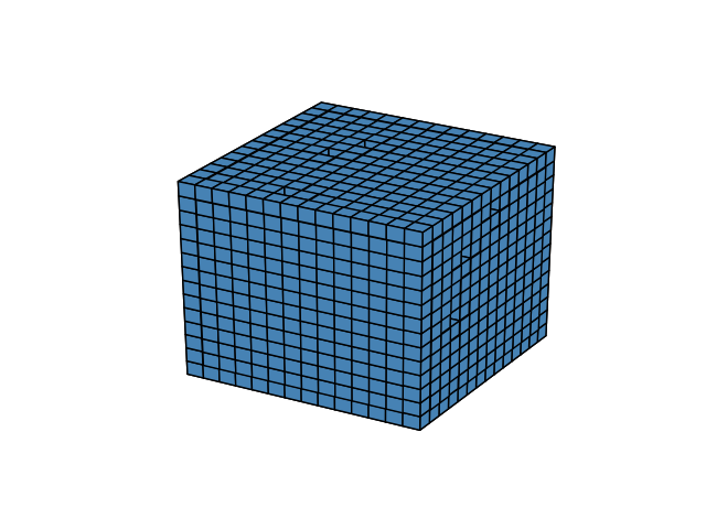
(b) $d=2.35$

Figure 25: Example of the space binning into voxels corresponding to the situation shown in Fig. 23. (a) The edge length of the cubic voxel is $d=1.85\,$fm. (b) The edge length of the cubic voxel is $d=2.35\,$fm.

Notice that whenever a fake empty voxel exists, the contiguous one will perhaps host two nucleons. This is because the nucleon that exceeds the $1.85\,$fm distance to the neighbor, say on the left, may have shorten the distance to the neighbor on the right. Thus, the number of occupied voxels will probably not match the number of nucleons. Fig. 24b shows a decrease in the number of occupied voxels (i.e. the volume) for $r>1.6\,$fm.

The space binning should be done wider in order to to avoid fake empty voxels. But, too wide voxels may include second neighbors. The most reasonable binning distance appears to be around the first minimum of $g(r)$ (see Fig. 23). That is, at some point between $2.15\,$fm and $2.35\,$fm.

A reasonable criterion for the space binning may raise from the Euler functional: the right binning distance should drive the $\chi$ functional to unity, that is, to a single compact region. This occurs at $d=2.35\,$fm for sure, as can be seen in Fig. 25b. It can be further checked from Fig. 24b that this binning allows the hosting of approximately two nucleons per voxels, meaning that the number of fake voids is negligible.

Appendix C The $E_{sym}$ fitting procedure errors

The accuracy of the fitting procedure was further tested according to the hypothetical expansion

$$\Delta E(\alpha)\simeq E_{sym}\,\alpha^{2}+\mathcal{O}(\alpha^{4})$$ (19)

where $\Delta E=E(\rho,T,\alpha)-E(\rho,T,\alpha=0)$. The odd-terms in $\alpha$ are excluded due to the exchange symmetry between protons and neutrons of the strong force lopez2014 . Fig. 26 shows the corresponding results for the explored densities.

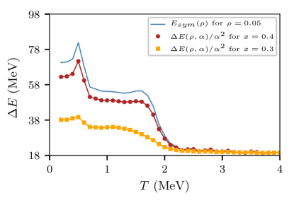
(a) $\rho=0.05$

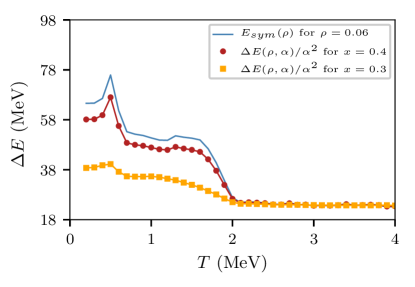
(b) $\rho=0.06$

(c) $\rho=0.07$

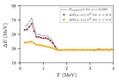
(d) $\rho=0.085$

Figure 26: Symmetry energy and the variation of internal energy $\Delta E(\alpha)$ as a function of the temperature, for nuclear matter with 6000 nucleons. The corresponding densities are indicated below each plot (units fm^-3). Rounded symbols correspond to $\Delta E(\alpha=0.2)$ or $x=0.4$. Squared symbols correspond to $\Delta E(\alpha=0.4)$ or $x=0.3$. The single line represents the fitting procedure (see text for details).

The current fitting procedure appears to be accurate if compared to the ratio $x=0.4$, but a noticeable bias is present for the ratio $x=0.3$. This means that the $\mathcal{O}(\alpha^{2})$ terms (that is, $\mathcal{O}(\alpha^{4})/\alpha^{2}$) may become relevant for proton fractions as low as 30%. Nevertheless, the fitting procedure always results in $\Delta E<E_{sym}$ (despite round-off errors), meaning that the higher order corrections should carry a negative sign. Fig. 27 shows the relative higher order discrepancy (in modulus) for $x=0.4$ and $x=0.3$, respectively.

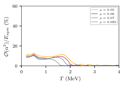
(a) $x=0.4$

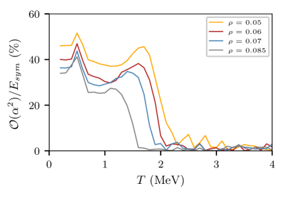
(b) $x=0.3$

Figure 27: (Color online) Relative difference for the high order terms with respect to the computed symmetry energy (in modulus and expressed in percentage) as a function of the temperature. The system corresponds to nuclear matter with 6000 nucleons. On the left, the explores densities at $x=0.4$. On the right, the explores densities at $x=0.3$. The corresponding densities are indicated in the insert (units fm^-3).

The higher order terms, at the pasta temperature range, represent roughly a 10% correction with respect to the first order approach of $E_{sym}$ for $x=0.4$, and around 40% for $x=0.3$, respectively. However, we checked over that both corrections have essentially the same pattern, regardless of a scaling factor.

Although the patterns shown in Fig. 27 and Fig. 21 are very similar, the former exhibits a local maximum within the temperature range $1-2\,$MeV. This maximum appears after the computation of $E_{sym}-\Delta E(\alpha)/\alpha^{2}$. It can be seem from Fig. 26 that the difference in the slopes between $E_{sym}$ and $\Delta E(\alpha)$ is responsible for this phenomenon. Thus, the rate at which $E_{sym}$ jumps from the high temperature regime to the pasta regime cannot be currently analyzed through the first order approach in Eq. (19), but through the higher order terms.

References

- (1) B.A. Li, L.W. Chen and C.M. Ko, Phys. Rep. 464, 113 (2008).
- (2) B.A. Li, A. Ramos, G. Verde, and I. Vidana, Eds., Topical issue on Nuclear Symmetry Energy, Eur. Phys. J. A 50, 39 (2014)
- (3) K. Hagel, J.B. Natowitz and G. Röpke, Eur. Phys. J. A 50, 39 (2014)
- (4) J.A. López and S. Terrazas Porras, Nuc. Phys. A957, 312 (2017).
- (5) R. Wada, et al., Phys. Rev. C 85, 064618 (2012).
- (6) S. Kowalski, et al., Phys. Rev. C 75, 014601 (2007).
- (7) J. B. Natowitz, personal communication, Medellin, Colombia, (2015).
- (8) D.G. Ravenhall, C. J. Pethick and J. R. Wilson, Phys. Rev. Lett. 50, 2066 (1983).
- (9) P.N. Alcain and C.O. Dorso, Nuclear Phys. A 961, 183 (2017).
- (10) P.N. Alcain, P.A. Giménez Molinelli and C.O. Dorso, Phys. Rev. C90, 065803 (2014).
- (11) M. Hempel, et al., Nucl. Phys. A837, 210 (2010).
- (12) C.J. Horowitz, A. Schwenk, Nucl. Phys. A 776, 55 (2006).
- (13) M. Hempel, K. Hagel, J. Natowitz, G. Röpke, and S. Type, Phys. Rev. C91, 045805 (2015).
- (14) B.K. Agrawal, J.N. De, S.K. Samaddar, M. Centelles, and X. Viñas, Eur. Phys. J. A50, 19 (2014).
- (15) J.A. López and E Ramírez-Homs, Nuc. Sci. and Tech. 26, S20502, (2015)
- (16) P.A. Giménez Molinelli, J.I. Nichols, J.A. López and C.O. Dorso, Nuc. Phys. A 923, 31 (2014).
- (17) M. Hashimoto, H. Seki and M. Yamada, Prog. Theor. Phys. 71, 320 (1984).
- (18) D. Page, J. M. Lattimer, M. Prakash and A. W. Steiner, Astrophys. J. Supp. 155, 623 (204)
- (19) R. D. Williams and S. E. Koonin, Nucl. Phys. A435, 844 (1985).
- (20) T. Maruyama, K. Niita, K. Oyamatsu, T. Maruyama, S. Chiba and A. Iwamoto, Phys. Rev. C57, 655 (1998).
- (21) T. Kido, Toshiki Maruyama, K. Niita and S. Chiba, Nucl. Phys. A663-664, 877 (2000).
- (22) G. Watanabe, K. Sato, K. Yasuoka and T. Ebisuzaki, Phys. Rev. C66, 012801 (2002).
- (23) C.J. Horowitz, M.A. Pérez-García, J. Carriere, D.K. Berry, and J. Piekarewicz, Phys. Rev. C70, 065806 (2004).
- (24) C.O. Dorso, P.A. Giménez Molinelli and J.A. López, Phys. Rev. C86, 055805 (2012).
- (25) C.O. Dorso, P.A. Giménez Molinelli and J.A. López, in “Neutron Star Crust”, Eds. C.A. Bertulani and J. Piekarewicz, Nova Science Publishers, ISBN 978-1620819029 (2012).
- (26) J. A. López, E. Ramírez-Homs, R. González, and R. Ravelo Phys. Rev. C89, 024611 (2014).
- (27) A. Vicentini, G. Jacucci and V.R. Pandharipande, Phys. Rev. C31, 1783 (1985); R. J. Lenk and V. R. Pandharipande, Phys. Rev. C34, 177 (1986); R.J. Lenk, T.J. Schlagel and V. R. Pandharipande, Phys. Rev. C42,372 (1990).
- (28) P.N. Alcain, P.A. Giménez Molinelli, J.I. Nichols and C.O. Dorso, Phys. Rev. C89, 055801 (2014).
- (29) S. Plimpton, J. Comp. Phys., 117, 1-19 (1995).
- (30) S. Nose, J. Chem. Phys. 81, 511 (1984).
- (31) F.A. Lindemann, Physik. Z. 11, 609 (1910).
- (32) Z.W. Birnbaum, Journal of the American Statistical Association, 47, 425-441 (1952).
- (33) E. Gosset, Astronomy and Astrophysics 188, 258-264 (1987).
- (34) G. Fasano and A. Franceschini, Monthly Notices of the Royal Astronomical Society 225, 155-170 (1987).
- (35) G.J. Babu and E.D. Feigelson Astronomical Data Analysis Software and Systems XV (eds. C. Gabriel et al.), ASP Conference Series, 351, 127 (2006).
- (36) K. Michielsen and H. De Raedt, Phys. Rep. 347, 461 (2001).