Bayesian Optimization with Expensive Integrands
Abstract
We propose a Bayesian optimization algorithm for objective functions that are sums or integrals of expensive-to-evaluate functions, allowing noisy evaluations. These objective functions arise in multi-task Bayesian optimization for tuning machine learning hyperparameters, optimization via simulation, and sequential design of experiments with random environmental conditions. Our method is average-case optimal by construction when a single evaluation of the integrand remains within our evaluation budget. Achieving this one-step optimality requires solving a challenging value of information optimization problem, for which we provide a novel efficient discretization-free computational method. We also provide consistency proofs for our method in both continuum and discrete finite domains for objective functions that are sums. In numerical experiments comparing against previous state-of-the-art methods, including those that also leverage sum or integral structure, our method performs as well or better across a wide range of problems and offers significant improvements when evaluations are noisy or the integrand varies smoothly in the integrated variables.
1 Introduction
We consider two closely-related derivative-free black-box global optimization problems with expensive-to-evaluate objective functions,
| (1) |
and
| (2) |
where is a simple compact set (e.g., a hyperrectangle, simplex, or finite collection of points); is a vector belonging to a set ; is finite and inexpensive to evaluate with a known analytic form; and is expensive to evaluate, does not provide derivatives with its evaluations, and may be observable either directly or with independent normally distributed noise. We also assume in (2) that is integrable for each . Here, “expensive-to-evaluate” functions are ones that consume a great deal of time per evaluation, e.g., minutes or hours each, or whose number is otherwise severely restricted (see, e.g., sacks1989, booker1998). We treat as a black box and assume that it is continuous in and also in in problem (2) and well-represented by a Gaussian process prior (RaWi06) as described below, but make no other assumptions on its structure.
This pair of closely related problems arises in three settings:
-
1.
First, both (1) and (2) arise when optimizing average-case performance of an engineering system or business process across environmental conditions, where is the performance of system design under environmental condition , and represents the fraction of time that condition occurs. This arises, for example, when choosing the shape of an aircraft’s wing (MLA), the configuration of a cardiovascular bypass graft (marsden2010), or the parameters of an algorithm that dispatches cars in a ride-sharing service.
-
2.
Second, both (1) and (2) arise when we wish to optimize the expected value of a system modeled by a discrete-event simulation , where is random. In this setting, we may choose a random variable whose distribution we know, and for which we can simulate given . We may then define . Our objective becomes either if is discrete or if is continuous, and we can obtain noisy observations of by simulating with drawn from its conditional distribution given . This arises, for example, when building a transportation system to maximize expected service quality subject to stochastic patterns of arrivals through the day , which we can simulate given the total number of arrivals in a day . When used for variance reduction in simulation rather than optimization, this technique is known as stratification (glasserman2003monte).
-
3.
Third, (1) arises when tuning a machine learning algorithm’s hyperparameters by using k-fold cross-validation. In this application, is the error on fold using hyperparameters and our goal is to minimize . This problem arises more generally when optimizing average performance across multiple prediction tasks (bardenet2013collaborative, hutter2011sequential, swersky2013multi) and is called multi-task Bayesian optimization (swersky2013multi).
Although (1) and (2) can be considered jointly as maximization of an objective where is a measure, and our theoretical analysis will at times take this view, (1) and (2) have very different properties computationally and have been considered separately in the literature so we refer to them separately here.
Potential Solution Approaches:
Problems (1) and (2) may be solved by optimizing directly with a method designed for derivative-free black box global optimization of expensive and possibly noisy functions. These methods include Bayesian optimization methods (jones1998efficient, forrester2008engineering, brochu2010tutorial) and other surrogate-based optimization methods (barthelemy1993, torczon1997, shoemaker2014). Indeed, can be evaluated using multiple evaluations of by summing in (1) or with numerical quadrature in (2). However, the expense of evaluating is many times larger than for , especially if in (1) is large or numerical quadrature in (2) is performed accurately. This approach is inefficient because it is unable to adjust the computational effort spent on evaluating : it either evaluates it fully or not at all. This inefficiency is most apparent when the first evaluations of at indicate is substantially sub-optimal: the extra expense of fully evaluating is wasted.
These problems may also be solved by applying a black box global optimization method to noisy observations of obtained via Monte Carlo sampling. One may sample from and use as a noisy estimate of . This approach is inefficient because it ignores information about when building its surrogate for . This inefficiency is most apparent when the first two evaluations of are at the same or very similar . If is free from noise and varies slowly with , the second such evaluation provides little information beyond the first. This inefficiency could perhaps be mitigated by using Quasi Monte Carlo (QMC; see, e.g., glasserman2003monte) together with an optimization method (ideally a multifidelity one, e.g., forrester2007multi) that is tolerant to bias in its noisy observations, but even this would become inefficient when most of ’s variability is driven by values of not sampled until later in the QMC sequence.
These inefficiencies in optimization based on surrogate models of suggest one may create a more efficient method through surrogate models of , coupled with intelligent selection of points and at which to evaluate . williams2000sequential and swersky2013multi developed methods of this type for solving (1), and groot2010bayesian, Xie:2012 for solving (2). While these approaches can improve performance over modeling alone, we show in this article that they leave substantial room for improvement. Indeed, all of these previous approaches except Xie:2012 use heuristic two-step rules that choose first without considering , and then choose with fixed. As we show below, not considering and together causes these methods to perform poorly in certain settings, even sometimes failing to be asymptotically consistent. Moreover, these previous methods are insufficiently general: Xie:2012 requires and the kernel of the covariance of the Gaussian process to be Gaussian, and all previous methods require evaluations of to be free from noise, significantly restricting their applicability.
Contributions:
In this paper, we significantly generalize and improve over this previous work by developing a novel method, Bayesian Quadrature Optimization (BQO), that uses a one-step value of information analysis to select the pair of points at which to evaluate . This method is general and supports solving either (1) or (2) with noisy or noise-free evaluations of , and this support for noisy observations significantly expands the applicability of our approach within optimization via simulation. This algorithm is Bayes-optimal by construction when only a single evaluation of may be made. We also prove that it provides a consistent estimator of the global optimum of as the number of samples allowed extends to infinity in both the finite and continuum domain settings for the finite sum problem (1). Performing the one-step value of information analysis at the heart of BQO requires solving a challenging optimization problem, and we present novel computational methods that solve this problem efficiently, including a novel discretization-free method for estimating the gradient of the value of information, a new convergence analysis of a different and less efficient discretized scheme more closely related to past work, and a novel transformation that provides a more computationally convenient form of . We demonstrate that our algorithm substantially outperforms state-of-the-art Bayesian optimization methods when observations are noisy or the integrand varies smoothly in the integrated variables, and performs as well as state-of-the-art methods in the remaining settings. Our demonstrations use a variety of problems from optimization via simulation and hyperparameter tuning in machine learning. We also provide a robust implementation of our method at https://github.com/toscanosaul/bayesian_quadrature_optimization.
Our method improves over the previous literature in three ways: First, it is more general, as it is the first to allow noise in the evaluation of , the first to simultaneously support solving both (1) and (2), and allows general in contrast with groot2010bayesian and Xie:2012’s requirement that be a normal density. Second, it is more well-supported theoretically, as its one-step optimality justification contrasts with the heuristic justification offered in williams2000sequential, groot2010bayesian and swersky2013multi. (Xie:2012 is one-step Bayes-optimal for the special case of (2) that it considers.) Also none of these previous methods come with a proof of consistency, and williams2000sequential may fail to be consistent if a poor tie-breaking rule is chosen as we note below. Third, it provides better empirical performance in problems with noisy evaluations or when the integrand varies smoothly in the integrated variables, and performs comparably in other problems. We discuss this previous literature in more detail below.
This paper significantly extends the conference paper MCQMC, where an early version of the BQO method was referred to as Stratified Bayesian Optimization (SBO). We have re-named our method to reflect its more general ability to solve problems beyond the second use-case based on stratification described at the start of this section. Beyond that conference paper, the current paper includes proofs of consistency for both finite and continuum domains for the finite sum problem (1), a proof of convergence of the discretized computational method used in that paper, a new discretization-free computational method that is substantially more efficient in higher dimensions, and additional numerical experiments on new problems with new benchmark algorithms.
Detailed Discussion of Related Work:
williams2000sequential considers the problem (1) when is noiseless, and uses a small modification of the well-known expected improvement acquisition function (Mockus1989, jones1998efficient). Their acquisition function is a two step procedure which first uses expected improvement to choose by maximizing the conditional expectation of given the past observations, and then chooses by minimizing the posterior mean squared prediction error. This algorithm is not consistent for finite for the following reason: After has been evaluated for all , (but not necessarily all ), almost surely. This implies that the conditional expectation of is for all . If the tie-breaking rule used chooses the same on each iteration, then this method will fail to evaluate each infinitely often. lehman2004 considers minor modifications of the previous algorithm, and their M-robust algorithm can also fail to be consistent with a poor tie-breaking rule.
groot2010bayesian considers problem (2) when is noiseless, is Gaussian, and the kernel of the Gaussian process on is the squared exponential kernel. Its acquisition function is a minor modification of the active learning method ALC (cohn1996). Numerical experiments in that paper do not demonstrate an improvement over evaluating directly. While the method proposed for choosing is motivated by minimizing the expected variance of the objective after one evaluation, it does not do so optimally. Instead, like williams2000sequential, it chooses ignoring what will be chosen, and then chooses with fixed. This is in contrast with our approach, which chooses and jointly in a one-step optimal way.
swersky2013multi considers problem (1) when is noiseless, and uses a small modification of the expected improvement acquisition function (jones1998efficient). Like williams2000sequential and groot2010bayesian, and in contrast with our joint optimization approach, it first chooses ignoring , and then in a second step it chooses with fixed. Although one should typically choose to reduce uncertainty about , swersky2013multi instead chooses using an expected improvement criterion over even though we are not maximizing over . This can select points whose posterior mean of is high but posterior variance is extremely low, essentially wasting a measurement. This leads in turn to examples where the policy repeatedly samples the same and under-explores, as we discuss in the appendix (D). Our numerical experiments show this method can perform well in problems with a small number of homogeneous tasks, but tends to underperform significantly as the number of tasks increase.
Xie:2012 considers problem (2) when is noiseless, is Gaussian and independent, and the Gaussian process on has a squared exponential kernel. BQO generalizes the method in that paper to the significantly more applicable setting where can be noisy (required for application to optimization via simulation), with any (required for applications to cross-validation in machine learning) and any kernel (required for good performance on a wider variety of problems). These generalizations significantly increase the difficulty of the problem, because they preclude closed-form expressions used in Xie:2012. We also provide significantly improved computational methods: the discretized method used in Xie:2012 to optimize the acquisition function requires computation that scales exponentially in the dimension, preventing its use for more than dimensions, while our discretization-free method has sub-exponential scaling and numerical experiments demonstrate excellent performance on problems in up to dimensions. Although Xie:2012 does not provide theoretical analysis, one can see our convergence proof for the discretized method as addressing theoretical questions left unanswered by that previous work. We also go beyond Xie:2012 in extending our methodology to be fully Bayesian by sampling Gaussian process hyperparameters from their posterior distribution using slice sampling.
Other related work includes marzat2013, which considers a related but different formulation of (1) based on maximizing worst-case performance over a discrete set of environmental conditions. lam2008 considers a modification of williams2000sequential where the criterion used is for response surface model fit instead of global optimization.
Our consistency proof for the finite sum problem (1) is the first for any algorithm that evaluates instead of . Consistency of some Bayesian optimization algorithms that evaluate have, however, been shown in the literature. frazier2009knowledge proved consistency of the knowledge gradient algorithm for any Gaussian process for finite domains. Later bull2011 proved consistency of expected improvement for functions that belong to the reproducing kernel Hilbert space (RKHS) of the covariance function. The recent working paper bect2016 also contains consistency results for knowledge gradient and expected improvement over any Gaussian process with continuous paths.
Our BQO algorithm can be considered to be within the class of knowledge gradient policies (PowellFrazier2008), because it selects the () to sample that maximizes the expected utility of the final solution, under the assumption, made for tractability, that we may take only one additional sample. Work on knowledge gradient algorithms in other settings includes frazier2009knowledge, poloczek2017multi, wugradientsbo. Our discretization-free approach leverages ideas in particular from wugradientsbo. Our algorithm also leverages Bayesian quadrature techniques (o1991bayes), which build a Gaussian process model of the function , and then use the relationships given by the sum or integral to imply a second Gaussian process model on the objective .
The rest of this paper is organized as follows: 2 presents our statistical model. 3 presents the conceptual value of information analysis underlying the BQO algorithm. 4 describes computation of the value of information and its derivative, and presents the BQO algorithm in a practically implementable form. 5 presents theoretical results on consistency of BQO. 6 presents simulation experiments. 7 concludes.
2 Statistical Model
Our BQO algorithm relies on a Gaussian process (GP) model of the underlying function , which then implies a Gaussian process model over . Before presenting BQO in 3, we present this statistical model to provide notation used through the rest of the paper. The first part of our development is standard in Bayesian optimization (jones1998efficient) and Bayesian quadrature (o1991bayes), while the second part, in which a Gaussian process on the function’s integral or sum is obtained, is only standard in Bayesian quadrature.
We suppose that observing at provides an observation equal to optionally perturbed by additive independent normally distributed noise with mean and variance . To permit estimation, we require one of two additional assumptions on this noise: either that is constant across the domain; or that observing at also provides an observation of . The first assumption has been shown to be effective in a wide range of applications in the Bayesian optimization literature (snoek2012practical). The second is reasonable in discrete-event simulation applications in which is the average of a large batch of independent replications. In such applications, the difference between and its mean converges to a normal distribution by the central limit theorem as the batch size grows large, and can be estimated by dividing the sample variance of these samples by their number (kim:2007).
We assume that the function follows a Gaussian process prior distribution:
where is a real-valued function taking arguments (the mean function), is a positive semi-definite function taking arguments (the kernel), and are the hyperparameters of the mean function and kernel. contains when the variance of the observational noise is assumed to be unknown and constant. Common choices for and from the Gaussian process regression literature (RaWi06, murphy2012machine, goovaerts1997geostatistics, seeger2005semiparametric, bonilla2007multi) appropriate for problem (2) include setting to a constant and letting be the squared exponential or Matérn kernel. In the case of the finite sum (1), kernels from the intrinsic model of coregionalization are appropriate (seeger2005semiparametric, goovaerts1997geostatistics, bonilla2007multi) and will be discussed in 6.
Following work on fully Bayesian inference in GP regression (Neal:GPBayesian), we additionally place a Bayesian prior distribution on . This prior can regularize values of used in inference, pushing them toward regions of the space of hyperparameters believed to best correspond to the data. The prior can also be set constant if there is enough data to obviate such regularization.
We now discuss inference supposing that we have points in the historical data , where is a (possibly noisy) observation of with the conditional distribution given , described above. Within our inference procedure we sample from its posterior distribution given via slice sampling (radford2003Slice). One may also replace this sampling-based fully Bayesian treatment of by using the maximum a posteriori estimate (MAP), which sets to its posterior mode (murphy2012machine). This is less computationally intensive, but tends to be less accurate. The maximum likelihood estimate (MLE) of is a particular case of the MAP when the prior distribution on is flat.
Using this procedure to sample , we now describe computation of the posterior distribution on both and given . The posterior distribution on given at time is
where the parameters , can be computed using standard results from Gaussian process regression (RaWi06). To support later analysis, we provide these expressions here, suppressing dependence on in our notation:
| (6) | |||||
| (10) |
where
We now describe the posterior distribution on the objective function given . We assume that is written in its integral form (2). Results for (1) are similar, where the resulting expressions are obtained by replacing integration over by a sum over (or equivalently Lebesgue integration with respect to a counting measure). We denote by , , and the conditional expectation, conditional covariance, and conditional variance with respect to the Gaussian process posterior given and . By results from Bayesian quadrature (o1991bayes), for , we have that
| (11) | ||||
| (12) |
Ignoring some technical details, the first line is derived using interchange of integral and expectation, as in . The second line is derived similarly, though with more effort, by writing the covariance in terms of the expectation and interchanging expectation and integration.
3 Conceptual Description of the BQO Algorithm
Our BQO algorithm uses the statistical model described in 2 and samples sequentially. It chooses where to sample using a value of information analysis (Ho66). This analysis measures the expected quality of the best solution we can provide to (1) or (2) after samples, and how this quality improves with an additional sample of . In this section we describe this value of information analysis from a conceptual perspective in preparation for describing in 4 the novel computational methodology we create to make its implementation possible. This conceptual value of information analysis echos the use of value of information in Bayesian optimization in works on knowledge-gradient methods (frazier2009knowledge) and in problem (2) by Xie:2012. The value of information analysis we describe here generalizes Xie:2012 to support noisy observations, integrals with dependent normally distributed densities, non-normally distributed densities, and sums, and general kernels. While the generalization of the conceptual form of the value of information analysis from Xie:2012 to handle this richer class of problems is straightforward, it presents a host of new computational challenges that requires new methodology, as fully described in 4.
We conduct our value of information analysis assuming the hyperparameters are given, as is common practice in Bayesian optimization (swersky2013multi, reviewBO). Then, in the implementation of the BQO algorithm, because is unknown, we average this -dependent value of information over the posterior on . While in principle one could instead conduct the full value of information analysis acknowledging that is unknown, proceeding as we do provides substantial computational benefits.
To conduct this analysis, we first study the expected quality of the best solution we can provide. Given samples, , and a risk-neutral utility function, we would choose as our solution to (1) or (2),
where . This solution has expected value (again, with respect to the posterior after samples given ),
Consequently, the improvement in expected solution quality resulting from a sample at at time is
| (13) |
and we refer to this quantity as the value of information. Our Bayesian Quadrature Optimization (BQO) algorithm then is defined as the algorithm that samples where this value of information (marginalized over ) is maximized,
| (14) |
Here, the expectation is over the posterior on , as indicated by the subscript.
This policy is one-step Bayes optimal in the known-hyperparameter case (i.e., the prior on is concentrated on a single value), in the sense that if we can take one more sample before reporting a final solution then its sampling decision maximizes the expected value of at this reported final solution. It is not necessarily Bayes-optimal if we can take more than one sample, but we argue that it remains a reasonable heuristic, and our numerical experiments in 6 support this. It is also Bayes-optimal for the problem (1) in the known-hyperparameter case when the number of iterations converge to infinity, as we show in 5.
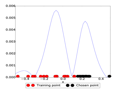
Figure 1 illustrates BQO, showing one step in the algorithm applied to a simple analytic test problem
| (15) |
where , , and . Direct computation shows . In the figure, we fix to a maximum likelihood estimate obtained using 15 training points.
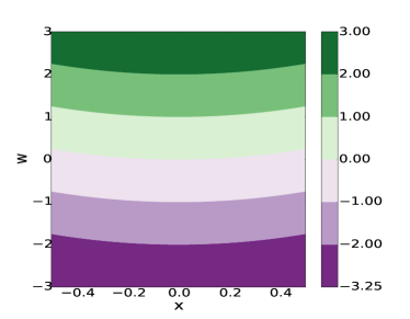
from by .
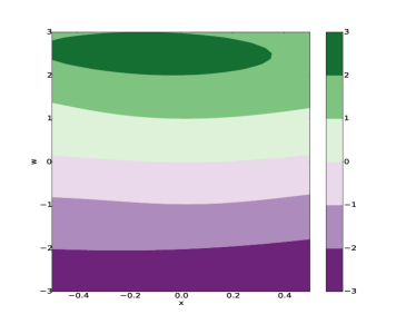
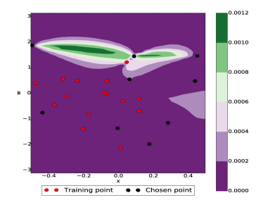
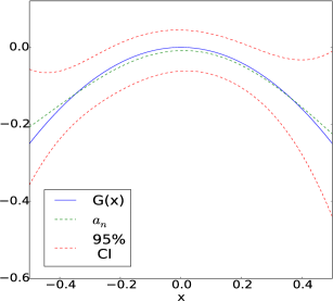
The figure’s first row shows the contours of (left panel) and BQO’s estimate (right panel) after evaluating at points chosen uniformly at random in an initial training phase, and at an additional points chosen by BQO. The second row’s left panel shows the value of information . The value of information is small near where BQO has already sampled, because it has less uncertainty about in this region. BQO’s value of information is also small for extreme values of , because its posterior on suggests that these are far from its maximum, and small for extreme values of because is small there. BQO’s value of information is thus largest for points that are far from previous samples, relatively close to the maximizer of ’s posterior mean, and have moderate values of . BQO samples next at the point with the largest value of information, near and . The second row’s right panel shows the posterior on . This posterior is accurate and almost perfectly estimates ’s maximizer.
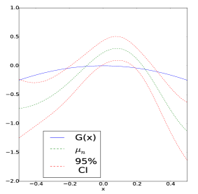
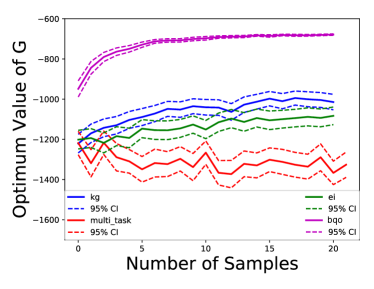
Figure 2 shows equivalent quantities for the knowledge-gradient (KG) method (frazier2009knowledge), after noisy evaluations of at points chosen uniformly at random in an initial training phase, and at an additional points chosen by KG. Like other traditional Bayesian optimization methods, KG models directly, ignoring valuable information from , and computes a value of information as a function of only while leaving the choice of to chance. As a consequence, KG’s estimates of and its maximizer have significantly more error than BQO’s estimates.
4 Computation of the BQO Algorithm
In this section we develop methods to compute the value of information (13) and its gradient, to support implementation of the BQO algorithm. We introduce a new and powerful method in 4.2 for computing unbiased stochastic estimators of the gradient of the value of information, which we refer to more briefly as stochastic gradients. These stochastic gradients are used within a stochastic gradient ascent method to optimize the value of information.
We also show in 4.4 how a deterministic discretized method for approximating the value of information and its gradient, first developed in Xie:2012 for the setting without noise and independent Gaussian and kernel, can be extended to our more general setting. When it was first proposed in Xie:2012 it lacked a theoretical analysis of its discretization error. To address this shortcoming, we demonstrate that this discretization error vanishes asymptotically when the discretizations are sufficiently well-designed. We refer to this method as the “discretized method,” and refer to the first method (which does not rely on discretization) as the “discretization-free method.”
We provide an analysis of the computational complexity of each method, showing that the time and space complexity of the discretization-free method scale better in the dimension of . In concert with this theoretical observation, empirical observations show that the discretized method is fastest when has one or two dimensions but is too slow to be practical in higher dimensions. In contrast, our numerical experiments (6) show that our novel discretization-free method is practical in dimensions as large as .
To simplify proofs, we assume that has the integral form defined in (2). As we mentioned in 2, results for (1) are similar, where the resulting expressions are obtained by replacing integration over by a sum. We also assume in our computation of the value of information that is given, as discussed in 3, and drop the dependence on from our notation (except in 4.3 where we write it explicitly to support a high-level summary of the BQO algorithm). Table 1 summarizes notation used in this section, including both notation introduced in previous sections and new notation defined later in this section.
| or | ||
| Value of information at time | ||
| History observed by time | ||
| Kernel of the Gaussian process prior distribution over the function | ||
| if , or | ||
| if for | ||
| Variance of the noise in evaluations of | ||
| conditional variance given |
4.1 Preliminary Representation of the Value of Information
In this section, we find a useful representation of the value of information (13) that will allow us to develop the discretization-free (4.2) and discretized (4.4) methods to approximate it and its gradient. We first observe that we can rewrite the value of information (13) as
| (16) |
This expression is not directly useful from a computational perspective, so we take one step further and find the joint distribution of across all conditioned on and for any . This is provided by the following lemma. The lemma is a generalization of Section 2.1 in frazier2009knowledge, and we include the proof in the appendix A.
Lemma 1.
There exists a random variable , whose conditional distribution given is standard normal, such that for all , with
The posterior mean of can be represented by
| (20) |
where for . We also have that
| (21) |
where .
The expressions in this lemma require that be known to compute the value of information. This is seldom true in practice, but this quantity can be estimated and the estimate used in its place. If the noise is homogeneous then it can be estimated by including it as a hyperparameter in our Gaussian-process-based inference. If each observation is an average of many i.i.d. replications, allowing the variance of the noise in each observation to be estimated with high accuracy, and we believe that the noise does not change abruptly in the domain, then we can use the mean of the variance estimates from previous observations as our estimator of . Finally, if we are in neither of these situations, then we can use the approach developed in Kersting2007 in which a Gaussian process is used to estimate the variance of heteroscedastic noise across the domain.
We now use Lemma 1 to estimate the value of information and its gradient in the next subsection.
4.2 Discretization-Free Computation of the Value of Information and its Gradient
In this subsection, we provide unbiased and strongly consistent Monte Carlo estimators of the value of information and its gradient. Our techniques use the envelope theorem (milgrom) and were inspired by wugradientsbo, which uses this theorem to build an unbiased estimator of the gradient of the knowledge-gradient in a different setting.
First, Lemma 1, equation (16), and the strong law of large numbers show that if are independent standard normal random variables, then
is an unbiased and strongly consistent estimator of the value of information . The inner optimization problems can be solved using standard optimization methods such as LBFGS (byrd:1997) or Newton methods (if the Hessian of the kernel exists). Gradients of the inner optimization problem’s objective can be computed using (24).
We now build an unbiased and strongly consistent estimator of where , , and give sufficient conditions for existence of . We use the envelope theorem (milgrom), along with the following lemma, which shows some smoothness properties of and . The proof of this lemma may be found in A.
Lemma 2.
We assume is constant, and the kernel of the prior distribution on is continuously differentiable and bounded. We also suppose there is a non-negative function such that is finite for all , and for all and . Then:
-
1.
and are both continuously differentiable for any if .
-
2.
For any , is continuously differentiable with respect to if and is continuously differentiable.
The condition in the previous lemma is always true in the noisy case, as shown by (10). In the noiseless case, can be zero only if is a previously measured point.
The following lemma shows how to compute stochastic gradients of and allows us to optimize with a stochastic gradient ascent method.
Lemma 3.
Suppose that the hypotheses of Lemma 2 on and are satisfied. Also assume that for a given , is almost surely a singleton, where is a standard normal random variable. Also assume and is continuously differentiable at and . Let be independent standard normal random variables. Then
where . Furthermore, for all .
Proof.
Let be a standard normal random variable, and where and . By Lemma 2, is continuously differentiable, and so by the envelope theorem (milgrom, Corollary 4),
where and the dependence of on , is ignored when taking the gradient.
We now show that . First observe that if is a real number such that , by the envelope theorem, we then have that,
Furthermore, we have that
where , which is finite because is continuously differentiable and is a compact set. Consequently, .
By Corollary 5.9 of bartle, . Finally, the first claim of the lemma follows from the strong law of large numbers.
∎
As a reminder, we assumed that the objective function has the integrated form at the beginning of the section. In the case of the finite sum (1), the assumptions we have made in Lemma 3 and Lemma 2 may no longer hold. In particular, will typically not exist for where , and so may not exist either (see Lemma 1). However, our approach remains applicable in this setting: we use to maximize for each , and then easily solve observing that is a finite set. Using in this way requires showing similar results to the ones presented in this section to compute stochastic gradients of with respect to for any fixed , under the assumption that and are sufficiently smooth for any . We do not include these results here, because their proofs follow the same ideas already presented.
4.3 Computation and Complexity of the BQO Algorithm
In this section, we summarize computation of the BQO algorithm, which combines the tools developed in previous sections, and discuss its complexity. First, recall we previously described methods for obtaining unbiased samples of and using a fixed value of . Because was fixed, we suppressed it in our notation, but here we indicate it explicitly, writing these values as and and their estimators as and respectively. We will use these within a stochastic gradient algorithm, ADAM (adam), for solving problem (14), i.e., for maximizing . Within this stochastic gradient algorithm, each stochastic gradient is obtained by first taking independent samples from the posterior distribution on given using slice sampling, and then computing , where each uses a single independent standard normal random variable (so as defined Lemma 3). We use a similar approach in the final step of our algorithm to select a point with maximal posterior mean , except that the only source of randomness in our stochastic gradient estimator is .
The BQO algorithm using this approach is summarized in Algorithm 1.
Observe that in the noise-free case, is not differentiable at any previously evaluated point , as shown by the last equation of Lemma 1. The set of previously evaluated points, however, is finite and so we can still use ADAM by perturbing the algorithm’s current iterate whenever it resides at a non-differentiable point. A similar idea can be found in jordan:saddle.
Finally we discuss BQO’s time and space complexity, assuming we use it to select points to sample. To select each point to sample, we use Algorithm 1, which runs the ADAM algorithm for iterations. Each iteration requires a stochastic gradient computed using independent standard Gaussian random variables, independent samples from the posterior on (let be the number of iterations of slice sampling used for each), and runs of LBFGS to maximize . Let be the number of steps in a single run of LBFGS, where each step requires an evaluation of , , and their gradients. Let be the complexity of computing the kernel and its gradient, and let be the complexity of computing (24),, and for all .
With this notation, we show in the appendix (B) that the BQO algorithm has time complexity and space complexity .
The integrals in (24), , and do not necessarily have closed-form expressions. While we might estimate them via Monte Carlo or numerical integration, this can be inconvenient and increase computational cost. Consequently it may be better to first perform a change of variables from to another for which integrals may be evaluated in closed form. One such transformation, to the Gaussian distribution, is discussed in the appendix C. In addition, a change of variables from to induces a change from to some other , which might change more slowly with (requiring fewer samples to model it) or be better modeled by a Gaussian process. We illustrate this change of variable technique in our numerical experiments, in the inventory (6.6) and Citi Bike (6.3) problems.
4.4 Discretized Computation of the Value of Information and its Gradient
In this section we describe an alternate approach to that in 4.2 for estimating the value of information and its gradient. It uses a discretization of . Although this approach was already considered in Xie:2012, which presents a particular case of our method for the integral objective (2) in the noise-free setting with an independent Gaussian and Gaussian kernel, we extend this analysis by generalizing it to our setting and showing that a sequence of increasingly fine discretizations produces a sequence of estimators whose estimates converge to the value of information. Thus, these estimators, while biased, are strongly consistent. In practice, computational intractability limits this approach when has more than dimensions. This lack of scalability is also demonstrated by a complexity analysis we present at the end of this subsection.
Lemma 4.
We assume that is continuous for all , , is bounded, and is a constant. Suppose that we have an increasing sequence of finite discretizations of , such that is dense in . Then
The proof of this lemma may be found in A. A sequence of discretizations that satisfy the properties of the lemma can be built by considering the rationals, as we do in the proof of Theorem 5.
Using the previous lemma, we have that , where , , and is defined by
where and are any deterministic vectors, and is a one-dimensional standard normal random variable. We can then approximate the value of information by for some . By convenience, we denote by and by for each in . If , which is possible if is a finite set, then the approximation is exact.
Algorithm 1 of frazier2009knowledge applied to , gives a subset of indexes from , such that , where , for , and are the standard normal cdf and pdf, respectively. This shows how to approximate the value of information using the discretization of .
We now show how to approximate the gradient of the value of information using the discretization of . Observe that if , and so . On the other hand, if , one can show via direct computation that . Consequently, we only need to compute for each in . Another direct computation shows that , where
Complexity of the Discretized Version of the BQO Algorithm.
Here we discuss the time and space complexity of a version of BQO based on discretized computation of the value of information and its gradient. We use the same notation and a similar analysis to that in the previous section. As a reminder, is the complexity of the computation of the kernel and its gradient, and is the complexity of computing , and for all . We sample parameters from the posterior on , running slice sampling for at most iterations for each, and we optimize the value of information with the ADAM algorithm for at most iterations. If we use a uniform discretization of size where is the dimension of , the time complexity of the BQO algorithm run for iterations is , and the space complexity is . Thus if increases, the time complexity and space complexity increase exponentially. This makes this method impractical when .
5 Asymptotic Analysis for BQO
In this section, we show consistency of BQO. We show that if and are finite, is finite or a closed box in , the integrand function follows a Gaussian process prior with continuous paths for a fixed , and the prior on the hyperparameters of the kernel is concentrated on a single value, then as the number of iterations of the algorithm tends to infinity, the optimal solution given by the BQO algorithm converges in expectation to an optimal solution . We omit the explicit dependence of the expressions on since the prior on is assumed concentrated on a single value.
We state two consistency results, one for continuum (Theorem 1) and the other for finite (Theorem 2). The proofs for both results may be found in the appendix. The proof for finite has a similar structure to the proof of consistency for the knowledge-gradient method for finite domains in problems without integrated objectives from frazier2009knowledge. We present a proof for the finite case partly because finite arises in practice, and partly because it is substantially simpler than the continuum case and provides a starting point for understanding the continuum proof. Our proof for the continuum goes substantially beyond the techniques required for the finite case, and develops techniques that may also be useful for proving consistency of other Bayesian optimization methods in continuum settings. Consistency of Bayesian optimization in continuum settings has been largely unexplored, with the authors being aware of only two other papers on this topic: The working paper bect2016 contains consistency results for Bayesian optimization algorithms over Gaussian processes with continuous paths in the continuum setting; and bull2011 proved consistency of expected improvement for functions that belong to the reproducing kernel Hilbert space (RKHS) of the covariance function in the continuum setting, though Driscoll’s Theorem (beder2001) shows that, under some regularity conditions, sample paths of the Gaussian process almost surely do not belong to the RKHS.
We first introduce notation needed for the theorems. Define . Define the set , where is the set of functions defined on , and is the set of positive semidefinite functions defined on . We define the set as
We first state our result for continuum and prove it in the appendix E.2,
Theorem 1.
Suppose that , for all , is a finite set, and the probability space is complete. Assume . We assume that the function is continuous in for all , and there exists such that for all and . Then
where indicates expectation with respect to the distribution over sampling decisions induced by BQO.
We also state our result for finite and prove it in the appendix E.1,
Theorem 2.
Suppose that and are finite. Assume . We have that
6 Numerical Experiments
In this section we present numerical experiments motivated by applications in operations research and machine learning. We compare the BQO algorithm against baseline Bayesian optimization algorithms and algorithms from the literature designed for the specific problems considered. These experiments illustrate how the BQO algorithm can be applied in practice, and demonstrate it performs at least as well as these benchmarks on all problems considered, and often much better.
We compare on seven test problems: a test problem with a simple analytic form (6.1); a composition of Branin functions (6.2) used in williams2000sequential; a realistic problem arising in the design of the New York City’s Citi Bike system (6.3); cross-validation of convolutional neural networks (6.5) and recommendation engines (6.4); an inventory problem with substitution (6.6); and a collection of problems simulated from Gaussian process priors (6.7) that provide insight into how the benefit provided by BQO is determined by problem characteristics, and that identify problems where BQO is most helpful.
As benchmark algorithms we consider the multi-task algorithm in Section 3.2 of swersky2013multi and the algorithm of williams2000sequential, which both place a Gaussian process prior on , as BQO does. In addition, we consider two baseline Bayesian optimization algorithms: the knowledge-gradient (KG) policy of frazier2009knowledge and the Expected Improvement criterion of jones1998efficient, which both place the Gaussian process prior directly on . The KG policy is equivalent to BQO in problems where all components of are moved into . We also solved the problems from 6.1 and 6.3 with Probability of Improvement (PI) (brochu2010tutorial), but do not include these results because both KG and EI significantly outperform PI.
We now discuss the kernels used in these experiments. When implementing BQO and the benchmark algorithms in the Branin (6.2) and inventory (6.6) problems, we use the -Matérn kernel , where .
In the cross-validation problems (6.4, 6.5), we use the expected improvement algorithm with the -Matérn kernel, and the BQO algorithm (Algorithm 1 in 3) and multi-task Bayesian algorithm with the task kernel (swersky2013multi), which is the Kronecker product of a -Matérn kernel and a kernel defined only over the finite set . Specifically this kernel is defined by where , is the number of tasks, and are real numbers, such that whenever and , and the matrix is symmetric and positive definite.
In the analytic test problem (6.1), Citi Bike problem (6.3), and the problems simulated from Gaussian process priors (6.7), we implemented BGO and the benchmark algorithms with the squared exponential kernel , where is the common prior variance and are the length scales parameters.
In the majority of our experiments (6.2 and 6.4-6.6) we implement BGQO using the discretization-free approach with fully Bayesian inference over hyperparameters (Algorithm 1 in 3). In the analytic test problem (6.1), the Citi Bike problem (6.3), and the problems simulated from Gaussian process priors (6.7), we use the discretized version (4.4) of the BQO algorithm. In these problems we also calculate the hyperparameters of the kernels, and , using maximum likelihood estimation following the first stage of samples. We do not use the discretization-free version of BQO in these problems because they were performed as part of an initial conference paper version of this work (MCQMC), and only the discretized version of BQO existed at that time. Benchmark algorithms in each problem were implemented using the same approach to hyperparameter estimation as used by BQO.
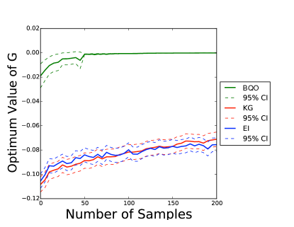
6.1 An Analytic Test Problem
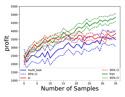
In our first example, we consider the problem (15) stated in 3. BQO is well-suited to this problem because evaluations of have much lower noise than those of . We do not compare against the multi-task algorithm (swersky2013multi) and SDE algorithm (williams2000sequential) because they can only be applied when the objective function is a finite sum. We do not compare against Xie:2012 because this problem has noisy evaluations. Figure 3 compares the performance of BQO, KG and EI on this problem, plotting the number of samples beyond the first stage on the axis, and the average true quality of the solutions provided, , averaging over 3000 independent runs of the three algorithms. We see that BQO substantially outperforms both benchmark methods. This is because BQO reduces the noise in its observations by conditioning on , allowing it to more swiftly localize the objective’s maximum.
6.2 Branin Function
In this example problem we compare BQO against the SDE (williams2000sequential) and multi-task (swersky2013multi, Section 3.2) algorithms. We consider the Branin problem proposed in williams2000sequential where ,
is the Branin function and . We define and . The joint distribution of is defined in Table 2. We maximize the function .
| 0.2 | 0.4 | 0.6 | 0.8 | |
|---|---|---|---|---|
| 0.25 | 0.0375 | 0.0875 | 0.0875 | 0.0375 |
| 0.5 | 0.0750 | 0.1750 | 0.1750 | 0.0750 |
| 0.75 | 0.0375 | 0.0875 | 0.0875 | 0.0375 |
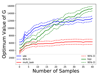
Figure 4 compares the performance of BQO, SDE and the multi-task algorithm on this problem, plotting the number of samples beyond the first stage on the axis, and the average true quality of the solutions provided, . We average over 100 independent runs of the BQO algorithm, 126 independent runs of the multi-task algorithm, and 230 independent runs of the SDE algorithm. We see that BQO substantially outperforms both the SDE and multi-task optimization benchmarks, despite the fact that these competing methods also model . We believe this is because SDE and the multi-task optimization algorithm both choose points using a heuristic rule that performs poorly in certain settings, as explained in the introduction, rather than using a one-step optimality analysis like BQO.
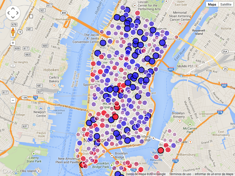
6.3 New York City’s Citi Bike System
We now consider a queuing simulation based on New York City’s Citi Bike system in which system users may remove an available bike from a station at one location within the city and ride it to a station with an available dock in some other location. The optimization problem that we consider is the allocation of a constrained number of bikes (6000) to available docks within the city at the start of rush hour, so as to minimize, in simulation, the expected number of potential trips in which the rider could not find an available bike at their preferred origination station, or could not find an available dock at their preferred destination station. We call such trips “negatively affected trips.”
We simulate the demand for bike trips on days from January 1st to December 31st between 7:00am and 11:00am. We use 329 actual bike stations, locations, and numbers of docks from the Citi Bike system. In our simulator, we choose a day at random from the 365 days of the year and then simulate the demand for trips between each pair of bike stations on that day using an independent Poisson process whose rate is given by historical data from that day in 2014 available from Citi Bike’s website (citibike). Travel times between pairs of stations are modeled using an exponential distribution with parameters estimated from this same dataset. If a potential trip’s origination station has no available bikes, then that trip does not occur, and we increment our count of negatively affected trips. If a trip does occur, and its preferred destination station does not have an available dock, then we also increment our count of negatively affected trips, and the bike is returned to the closest bike station with available docks.
We divide the bike stations into groups using k-nearest neighbors, and let be the number of bikes in each group at 7:00 AM. We suppose that bikes are allocated uniformly among stations within a single group. The random variable is the total demand for bike trips during the period of our simulation, summed over all pairs of bike stations. The distribution of is a mixture of Poisson distributions. Evaluations of for fixed are noisy due to additional sources of randomness beyond within our simulation.
We solve this problem with BQO, KG, EI and the multi-task algorithm. The multi-task algorithm cannot solve problems where the objective function is an infinite sum, as it is in this problem, so we modify the objective function it uses to a truncated expectation over finitely many values of . Because implementing the multi-task algorithm become computationally intractable when there are thousands of tasks, we restrict this truncated expectation to 181 values of .
Figure 5(a) compares the performance of BQO, KG, EI and the multi-task algorithm, plotting the number of samples beyond the first stage on the axis, and the average true quality of the solutions provided, , averaging over 300 independent runs of BQO, EI and KG, and 100 independent runs of the multi-task algorithm. We see that BQO quickly finds an allocation of bikes to groups that attains a small expected number of negatively affected trips. We believe that multi-task does poorly because of the large number of tasks, and its inability to leverage information across related tasks.
6.4 Hyperparameter Tuning in Recommender Systems
In this subsection and the following we consider optimization of a machine learning model’s hyperparameters where error is evaluated using cross-validation. Cross-validation is a method for estimating a machine learning model’s error. In more detail, -fold cross-validation randomly splits the training data into datasets of roughly equal size. Then, for each dataset (or “fold”), it trains the machine learning model holding out that data, and evaluates the error of the resulting estimates on the held out data. The average of these errors is called the cross-validation error, and is used as an objective in optimization of a machine learning model’s hyperparameters. In this approach, we minimize over , where is the error of the model with hyperparameters evaluated on the -th dataset .
In this subsection we consider the problem of optimizing hyperparameters for probabilistic matrix factorization (PMF) models used in recommender systems (mnih2008). We apply this PMF model to a dataset from arxiv.org (arxiv), with information about downloads from users on papers. We treat a user as providing a positive binary rating for a paper if that user downloaded the paper, which creates positive binary ratings.
We use -fold cross-validation to provide an estimate of the test error as a function of four PMF model hyperparameters: the learning rate, the regularizer, the number of epochs, and the matrix rank. We then use EI, BQO and the multi-task algorithm to choose these hyperparameters to minimize this cross-validation error. EI simply selects a set of hyperparameters at each step and evaluates all 5 folds, while BQO and the multi-task algorithm select an and a fold .
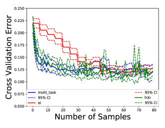
Figure 6(a) compares the cross-validation error of these algorithms, plotting the number of folds queried beyond the first stage on the axis, and the best error obtained, averaging over independent runs of BQO and multi-task, and of EI. We see that BQO and multi-task perform similarly, and both outperform EI. We conjecture that multi-task’s competitive performance in this problem is due to the small number of tasks and the homogeneity of the folds.
6.5 Hyperparameter Tuning in Convolutional Neural Networks
We consider the problem of training convolutional neural networks (CNNs) to classify images (cnncifar). We use -fold cross validation on the CIFAR10 dataset (cifar), which consists of 10 classes and 50,000 training images. We choose the network architecture described in the pytorch tutorial (pytorch), which consists of two convolutional layers, two fully connected layers, and on top of them a softmax layer for final classification. We tune the following hyperparameters: the number of epochs, the batch size, the learning rate, the number of channels in the first convolutional layer, the size of the kernel in the convolutional layers, and the number of hidden units in the first fully connected layer. The number of channels in the second convolutional layer is the number of channels in the first convolutional layer plus 10, and the number of hidden units in the second fully connected layer is 84.
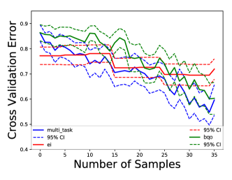
Figure 6(b) compares the performance of EI, BQO and the multi-task algorithm, plotting the number of folds queried beyond the first stage on the axis, and the best error obtained, averaging over independent runs of BQO and the multi-task algorithm, and of EI. We see that BQO and multi-task perform similarly, but better than EI. As in the recommender system problem, we conjecture that multi-task is competitive because of the small number of tasks and their homogeneity.
6.6 Newsvendor Problem under Dynamic Consumer Substitution
The newsvendor problem under dynamic consumer substitution is adapted from ryzin2001Stocking, and was considered in simopt. In this problem, we choose the initial inventory levels of the products sold, each with given cost and price . Our goal is to optimize profit.
A sequence of customers indexed by arrive in order and either buy an in-stock product, or decide to not buy anything. Here, is known. Customer assigns a utility to each product , and to the no-purchase option (indexed by ). Customer decides which product to buy, if any, by choosing the with the largest among the in-stock and the no-purchase option. Utilities for products () are modeled with the multinomial logit model, where , is constant, and are mutually independent Gumbel random variables with distribution function where is Euler’s constant. The utility for the no-purchase option is . In this problem, the objective function is defined as the expected overall profit considering the customers starting from a vector of initial inventory positions for each product. This profit is computed as sum of the prices of the products sold minus the cost of the initial inventory.
We consider the setting where there are customers and products whose costs are and dollars respectively and prices are and dollars respectively. We assume that is equal to for all .
We now describe how we use BQO in this problem. Fix a product . Observe that since for follows a Gumbel distribution with cdf , then is uniformly distributed on . Consequently, follows a gamma distribution where is the gamma cumulative distribution function. Now define the vector where . It is straightforward to simulate given , for example by noting that the distribution of is Dirichlet and independent of (see Theorem 2.1 of Section 2.1.2 of dirichletbook). Thus, simulating from this Dirichlet and multiplying by the given value of provides a sample of given . Alternatively, we can use a simple modification of Example 10e in Section 10.2 of rossSimulation. We can also simulate given that resides in an interval by acceptance-rejection sampling, or by simulating from a truncated gamma distribution, and then simulating conditioned on .
We then apply BQO with equal to the conditional expectation of the profit given and the initial inventory levels for each product. To observe this conditional expectation we average results from independent simulations, where the collection of values for are simulated conditioned on .
We similarly apply the multi-task algorithm with equal to the conditional expectation of the profit given the initial inventory level and that . Here, each is a rectangular region of values for , given by , , , and , where is the median of (this is the same for and ). For each observation of this conditional expectation we average independent simulations. The EI algorithm observes the profit without conditioning, averaging independent simulations.
In Figure 7 we compare the performance of EI, BQO and the multi-task algorithm, plotting the number of samples beyond the first stage on the axis, and the best profit obtained, averaging over independent runs of BQO, of multi-task, and of EI. We see that BQO outperforms the benchmark algorithms, and the multi-task algorithm underperforms the other algorithms considered.
6.7 Problems Simulated from Gaussian Process Priors
We now compare the performance of BQO against a benchmark Bayesian optimization algorithm on synthetic problems drawn at random from Gaussian process priors. By varying the parameters of the Gaussian process prior, we study how BQO’s performance relative to a benchmark (the KG algorithm) varies with problem characteristics, offering insight into the types of real-world problems on which BQO is likely to provide the most substantial benefit in comparison with using a traditional Bayesian optimization method.
These experiments show that the most important factor influencing BQO’s relative performance is the speed with which varies with . BQO provides the most value when this variation is large enough to influence performance, and small enough to allow to be modeled with a Gaussian process. Thus, users of BQO should choose a that plays a big role in overall performance, and whose influence on performance is smooth enough to support predictive modeling. These experiments also show that when settings are favorable, BQO provides substantial benefit, in some cases offering an improvement of almost . On those few problems in which BQO underperforms the benchmark, it underperforms by a much smaller margin of less than .
We now construct these problems in detail. Let on , where: is drawn, for each in a fine discretization of , independently from a normal distribution with mean and variance (we could have set to be an Orstein-Uhlenbeck process with large volatility, and obtained an essentially identical result); and is drawn from a Gaussian Process with mean and Gaussian covariance function . We then define by where the expectation is over , and by , where the expectation is over both and , is drawn uniformly from and is drawn uniformly from the discretization of . To observed , we draw 1 sample of and and average . (We also performed experiments, not shown here, that observed by averaging multiple samples, and found the same qualitative behavior.)
We thus have a class of problems parametrized by , , , and an outcome measure determined by the overall number of samples. Before displaying results, we reparametrize the dependence on and in what will be a more interpretable way. We first set to 1, as multiplying both and by a scalar simply scales the problem. Then, the variance reduction ratio achieved by BQO in conditioning on is approximately , with this estimate becoming exact as grows large and the values of become uncorrelated across . We define equal to this approximate variance reduction ratio. Thus, our problems are parametrized by the approximate variance reduction ratio , the overall number of samples, and by , which measures the speed with which varies with .
Given this parametrization, we sampled problems from Gaussian process priors using all combinations of and . We also performed additional simulations at for . Figure 8 shows Monte Carlo estimates of the normalized performance difference between BQO and KG for these problems, as a function of ( is the natural logarithm), , and the number of samples taken overall. The normalized performance difference is estimated for each set of problem parameters by taking a randomly sampled problem generated using those problem parameters, discretizing the domain into 2500 points, running each algorithm independently 500 times on that problem, and averaging across these 500 samples, where is the final solution calculated by BQO, and similarly for .
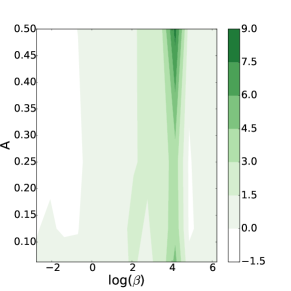
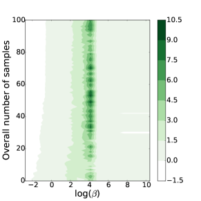
The normalized performance difference is robust to and the overall number of samples, but is strongly influenced by . BQO is always better than KG whenever . Moreover, it is substantially better than KG when , with BQO outperforming KG by as much as a factor of . For larger , BQO remains better than KG, but by a smaller margin. This unimodal dependence of the normalized performance difference on can be understood as follows: BQO provides value by modeling the dependence of on . Modeling this dependence is most useful when takes moderate values because it is here where observations of at one value of are most useful in predicting the value of at other values of . When varies very quickly with (large ), it is more difficult to generalize, and when varies very slowly with ( close to ), then modeling dependence on is comparable with modeling as constant.
7 Conclusions
We have presented a new Bayesian optimization algorithm, Bayesian Quadrature Optimization, designed for objectives that are sums or integrals of expensive-to-evaluate integrands. This method is derived from a conceptual one-step optimality analysis for which we provide novel computational techniques that support efficient implementation. We demonstrated that this method is consistent when the objective is a finite sum, and showed via extensive numerical experiments that it performs as well or better than the state of the art, providing substantial value when evaluations are noisy or the integrand varies smoothly in the integrated variables.
Acknowledgments
The authors were partially supported by NSF CAREER CMMI-1254298, NSF CMMI-1536895, AFOSR FA9550-15-1-0038, AFOSR FA9550-16-1-0046, and DMR-1120296.
References
Appendix
Appendix A Proofs of Results in Section 4
Proof of Lemma 1.
Proof.
Recall that we assume throughout 4 that has the integrated form (2). Results for (1) are similar with the resulting expressions obtained by replacing integration over by a sum. By equation (11),
| (22) |
where for .
Since conditioned on is normally distributed, then is also normally distributed. By the tower property,
and by the law of total variance,
Using the equation (22) and the previous expressions, we get the following formula for
| (23) |
where conditioning on , and , which ends the proof of the first part of the lemma.
Finally, we only need to show the last claim of the lemma. We have that if , or is not in , then , and then
where . Observe that in (23) the distribution of the left-hand side does not depend on the sign of . Thus, without loss of generality, we define equal to . If and is in , then it is easy to see that because .
∎
Proof of Lemma 2.
Proof.
We first show that and are continuously differentiable for each . In Lemma 1, we show that
and
Thus we only need to show that for all and are continuously differentiable on . is continuously differentiable because is constant.
We now show that is continuously differentiable for any . is bounded, and so is integrable with respect to for any because is integrable with respect to . Moreover, is differentiable with respect to , and is continuous on , and so it is bounded for any fixed because is compact. Consequently,
| (24) |
for all by Corollary 5.9 of bartle. Moreover, by Corollary 5.8 of bartle, is continuous on . This proves the first part of the lemma.
We now prove the second part of the lemma. Using a similar argument with the hypothesis that , and Corollaries 5.8 and 5.9 of bartle, we can show that is continuously differentiable for any x. Thus, using that is continuously differentiable, we can conclude that is continuously differentiable with respect to .
∎
Proof of Lemma 4.
Proof.
First, we show and are both uniformly continuous in . By Lemma 1,
and
Thus we only need to show that is continuous for all because is compact. The continuity follows from the Corollary 5.7 of bartle.
and are both bounded on because they are both continuous on a compact set, and so . Consequently by the monotone convergence theorem,
| (25) |
Appendix B BQO’s Time and Space Complexity
In this section, we discuss BQO’s time and space complexity, assuming we use it to select points to sample. To select each point to sample, we use Algorithm 1, which runs the ADAM algorithm for iterations. Each iteration requires a stochastic gradient computed using independent standard Gaussian random variables, independent samples from the posterior on , and runs of LBFGS to maximize . Let be the number of steps in a single run of LBFGS, where each step requires an evaluation of , , and their gradients. Let be the complexity of computing the kernel and its gradient, and let be the complexity of computing (24),, and for all .
To obtain a sample of from its posterior, we run slice sampling for at most iterations. To obtain a sample of from its posterior, we run slice sampling for at most iterations. Each iteration of slice sampling requires computing the likelihood of the data given the candidate parameters for the model. Computing the likelihood requires first computing , which requires kernel evaluations, each of which has complexity . It then requires computing the Cholesky decomposition of (which has complexity ) and solving a triangular system of equations involving this Cholesky decomposition (which has complexity ). Thus, each iteration of slice sampling has time complexity and space complexity , and the total complexity of sampling once using slice sampling is . Since we obtain samples for each value of from to , the total complexity due to sampling is in time, and in space.
Now, for each iteration of the ADAM algorithm, we optimize using LBFGS for at most iterations where is a sample of the hyperparameters of the model and is a sampled Gaussian random variable.
For each point visited within this optimization, we compute and its gradient, which requires computing and its gradient (see Lemma 1). This has time complexity , because the computation of each of the values of and their gradients is , giving the term. We then compute the matrix product involving using the pre-computed Cholesky decomposition of by solving a triangular linear system with complexity . (The complexity of computing the Cholesky decomposition of for this has already been accounted for above.)
For each point visited in the optimization we also compute and its gradient with respect to . To do this, we compute and its gradient with respect to , and . In doing so, we re-use the previously discussed computation of the terms and their gradients, and computation of the matrix product of and the inverse of the Cholesky decomposition of . The additional computation required is the matrix product of this same inverse of the Cholesky decomposition of with , which does not depend on and can be performed only once per optimization of , saving a factor of below. This extra computation introduces an additional time complexity incurred once per optimization of .
Consequently, the overall complexity due to optimizing within the ADAM algorithm for a single (but not including the complexity of sampling and computing the Cholesky decomposition of ) is in time, and in space. This computation is repeated for ranging from to , and has overall time complexity and space complexity .
By the previous two paragraphs, we conclude that the BQO algorithm has time complexity and space complexity .
Appendix C Closed-Form Expressions for the Gaussian and Squared Exponential Kernel Case
In this section we give closed-form expressions for and its gradient to compute BQO and its gradient when we use the squared exponential kernel , and
| (27) |
where , and is the density of a normal random variable with mean and variance .
The previous assumptions are quite common, for example they are assumed in Xie:2012. Moreover, we can always transform a problem of the form to a new problem of the form where is of the form given in (27) under suitable conditions. The procedure and necessary conditions are:
-
•
Denote the continuous density of by , where is a random vector such that .
-
•
Assume that we can compute or estimate the marginals of the random vector : for all .
-
•
Denote the inverse of the distribution function of a standard Gaussian random variable by . We have that for all . Thus,
-
•
We assume that is positive definite, and can be computationally estimated.
-
•
We have that .
-
•
Define , where is the ith component of the vector for all . Let denote the Jacobian computed from . Assume that does not vanish identically. By the change of variables theorem, we have that
where and is the ith entry of .
This shows how to transform a general problem to a problem with density given by (27), and the conditions under which this is possible. However, we do not always want to use this transformation because the correlation between and can be too small, which may not be optimal for BQO as we discuss in 6.7.
We now compute the closed-form expressions of and its gradient. We have that
for . Thus, we only need to compute for any and , which is given by the following equations,
This shows how to compute . We now compute the gradient of . Observe that
where is the derivative respect to the jth entry of . Consequently,
and
which shows how to compute the gradient of .
Appendix D Illustration of Poor Performance of the Multi-Task Algorithm
In this section we give an example where the average multi-task algorithm presented in Section 3.2 of swersky2013multi is inefficient, and we show that the BQO algorithm does not have that problem.
Let , , and , if . We want to maximize
We assume that , and has been evaluated. In addition, we suppose that for , for some , and their correlation is equal to zero. By equation 15 in jones1998efficient, we have that
if , where , and is the posterior variance of . Consequently,
and
where .
Suppose that in the next iteration we choose again a point of the form , and , thus we have that
and
where . Similarly, we can see that if we keep choosing points of the form , we are going to have that
and
where if .
Observe that
uniformly on if . Consequently, for large, we have that
if , and so we can only choose a point of the form until we have evaluated all the different points of the form , which is clearly inefficient when is large.
We now show that the BQO algorithm does not have that problem. Observe that if ,
and by Theorem 3 we have that for all , and thus the BQO algorithm chooses to evaluate .
Theorem 3.
We have that
if for all
Proof.
The proof is a direct consequence of Lemma 1 and the Vitale’s extension of the Sudakov-Fernique inequality (vitale2000).
∎
Appendix E Consistency of BQO
In this section, we prove the two consistency results: Theorem 1 and Theorem 2 of 5. To support the proofs of our theorems, we embed BQO within a controlled Markov process framework. We denote the probability space by , and assume it is complete. The action space is the domain of , which is , where is a subset of . The state space is the set of possible parameters of the Gaussian process on . More formally, if we denote by , the state space is defined by , where is the set of functions defined on , and is the set of positive semidefinite functions defined on .
The discrete-time dynamic system, which shows how the posterior parameters change when a new observation is obtained, is given by
where is the chosen point to measure at stage , , and is defined by
and
where is the variance of the sample of , e.g. where .
We now define a sequence of value functions by
where is the number of times that we can evaluate , is the class of admissible policies (a policy is a sequence of maps , where each maps parameters of the Gaussian process into the domain of ), and conditioning on means that where .
Similarly, we define the value of a policy as
An optimal policy given optimizes .
We denote the weighted sum of a function over by its Lebesgue integral respect to . Given , we denote the parameters of the induced GP on by , where the mean is and the covariance is . Observe that the integrals are sums because is finite.
We define the set as
We summarize the notation that is used in this section:
Observe that
We do not write the specific dependence on a policy when there is no confusion.
E.1 Consistency of BQO for Finite Domains
In this subsection, we prove a slightly stronger result (Theorem 4) whose proof implies Theorem 2. All the results of this subsection assume that both and are finite.
Theorem 4.
Suppose that and are finite. For each , we have that
Proof.
We first note that the limit of exists by Lemma 5. Denoted it by . Furthermore, is non-decreasing in and bounded above by Lemma 7, and so by Fatou’s lemma we have that . By Lemma 6, under the BQO policy a.s. for all . Thus,
and by Lemma 7. This ends the proof because .
∎
Lemma 5.
For any , and policy , we have that converges almost surely pointwise to , where and .
Proof.
This is proof is strongly based on frazier2009knowledge. We first show that the limit exists for any pair of points . Let where , and
We only need to show that converges a.s. since is a linear transformation of . We may write the components of as the conditional expectation of an integrable random variable with respect to (the smallest algebra generated by the information at time ) by and . Thus is a uniformly integrable martingale and hence converges a.s. (see Kallenberg1997). Thus the limit exists a.s. because the domain of is finite. Furthermore, since the limit of kernels is a kernel, we must have that is semi-positive definite.
∎
Lemma 6.
Under the BQO policy, if and is finite, then a.s. where is the limit of , and
Proof.
Define the events for any , , where is the limit of the parameters of the GP model, and define the Q-factors
For any , we define the events:
By Proposition 2, , and so is the event that for , and for . We will show that if , and so we will have that .
Let . Assume that . By contraposition of Lemma 8, there exists a measurable set such that , and for each , we have that there exists for each such that the BQO policy does not sample for .
Fix , and define . Given that and for and , there exists , such that
Thus the BQO policy must sample from at time , which contradicts the statement that the BQO policy never samples from at time . Consequently, , and so for all almost surely. By Lemma 9, we conclude that almost surely, as we wanted to prove.
∎
Lemma 7.
is non-decreasing in and is bounded above. For any policy , is non-decreasing in and is bounded above. Furthermore, .
Proof.
First, we prove that is non-decreasing in and bounded above. Observe that then
and this difference is not negative by Proposition 1. This shows that is non-decreasing.
Now, we show that . We have that for any policy ,
and then .
We now show that is non-decreasing in for any stationary policy. We have that and then
and this difference is not negative by Proposition 2.
∎
Proposition 1.
For and ,, we have that for all . Furthermore, for all states .
Proof.
This proof is based on a similar proposition in frazier2009knowledge. We first show that . We proceed by induction on . For , we have that , and by Jensen’s inequality
where the penultimate equality follows by Lemma 1.
Now, we prove the induction step. For ,
where the second equality follows from the dynamic programming principle.
In the last equation both points and are inerchangeable, in the sense that it does not matter the order in which and are chosen. Thus, we have that
where , and are the new parameters of the posterior Gaussian process after observing and choosing .
By the induction hypothesis,
as we wanted to prove.
Finally, take the extra measurement to be the measurement made by the optimal policy in state s, and thus by the first part of the proposition we conclude that .
∎
Proposition 2.
Let be a stationary policy, and . We have that .
Proof.
We proceed by induction on . Consider the base case, By Jensen’s inequality we have
where , and is the variance of the observations of .
Now consider the induction step. For , we assume that if , we have that for all parameters . Thus,
as we wanted to prove.
∎
Lemma 8.
If the policy samples from infinitely often almost surely, then almost surely under .
Proof.
Note that there exists a sequence of i.i.d. normal random variables with mean zero and variance such that we observe the -th time that is queried. By the strong law of large numbers, we have that there exists a measurable set of probability one such that converges to the zero random variable as goes to infinity. By hypothesis, there exists a measurable set with probability one such that samples from infinitely often. Consequently, has probability one.
Fix . Consider the observations where , and . So, we have that converges to , and then the posterior distribution of given does not depend on the noisy observations of . Consequently, we have that if , then
This ends the proof.
∎
Lemma 9.
Let . If is finite and for all , then .
Proof.
Suppose that and . Fix any and . We will show that for every , where
We reorder the index set such that . For a standard univariate normal random variable , we have that
Thus, using that , we have that
which implies that for almost every in Taking the limit as , by the bounded convergence theorem, we have that
and so a.s., which implies that .
For all , we have that
and so
By recursion, we conclude that for all , , we have that
Consequently, we have that for all
Denote by , we have that for all ,
Consequently, the vector has a covariance matrix with all entries equal to
Now define a normal random vector . Conditioned on , it has mean vector , and covariance matrix with all entries equal to . Consequently, is equal in distribution to .
We then have that
Then
which ends the proof. ∎
E.2 Consistency of BQO for Continuum Domains
Theorem 5.
Suppose that , for all , and . Let . We assume that the function is continuous in for all , and there exist such that for all and . We then have that
As we did in the appendix E.1, we analyze the problem with a dynamic programming framework, and use the same notation defined there. In addition, we assume without loss of generality that . All the results of this subsection assume that is finite.
We introduce the following notation:
| is | a finite set of A | |||
| is | ||||
Observe that
We should note that Lemma 7 proved in the appendix E.1 under the assumption that we can only choose a finite number of alternatives, holds under the assumption that we are optimizing over a finite set and we can choose any alternative in a compact set.
Proof of Theorem 5.
Proof.
Assume without loss of generality that . Let be an increasing sequence of sets defined by
It is clear that , and Let be a sequence of real numbers defined by
By Lemma 10 and the Monotone Convergence Theorem applied to we have that (note that the expectation of is finite by Lemma 11)
By Lemma 7, we have that
and then
| (28) |
thus by Theorem 6 and Lemma 7,
By the Monotone Convergence Theorem applied to and by Lemma 10, we have that
∎
Lemma 10.
Assume that , and . , where are the sets defined in the proof of Theorem 5.
Proof.
Let and . There exists such that
because is a continuous function in a compact set. Let such that whenever . Using the completeness of the rationals, we have that there exist ,, and such that , , and if ,
and then
which implies that if ,
and then almost surely.
∎
Lemma 11.
Let be an admissible policy, and . We have that, given a finite or compact set of and ,
Proof.
Let be the density of a normal random variable with mean zero and variance where is the point chosen by at iteration , we have that
| (30) |
where This shows that .
∎
Theorem 6.
Let be a finite set of . Suppose that , and . We have that
Proof.
We first note that the limit of exists a.s. by Lemma 13, and we denote it by . By Lemma 15, under the BQO policy a.s. Furthermore, is non-decreasing in and bounded above by Lemma 7, and so by Fatou’s lemma we have that . Thus, for any ,
and by Lemma 7. This ends the proof because .
∎
Lemma 12.
Let be the Reproducing Kernel Hilbert Space (RKHS) associated to any isotropic kernel defined in , where , we have the following:
-
1.
Consider the operator defined by
where , and
We have that , and
-
2.
Suppose that is continuous for any . Consider the operator defined by
where , and
We have that , and for all .
-
3.
where
-
4.
-
5.
for any if is in .
Proof.
-
1.
Define . It is easy to see that:
Furthermore, it is well known that in that case is a projection onto the space generated by
consequently we have that . Similarly, we can see that .
-
2.
Define the kernel for , and let be its RKHS. Define
where and .
Observe that if , and for all , we have that
where is the ith entry of .
Now take for some , and . Consider a sequence of points such that for all . Let be the kth entry of . Thus, we have that where is the kth entry of . By the previous result for all ,
and so
Now observe that by the previous equation and using that is positive definite,
as we wanted to prove.
-
3.
The proof is a simple consequence of the definition of .
-
4.
We have that
-
5.
It follows from the proof of Corollary 4.36 of steinwart2008svm.
∎
Lemma 13.
Suppose that . Given a finite set . Consider any , and policy . We have that the following happens almost surely:
-
1.
converges to , and for all , . Furthermore, for all , and .
-
2.
The convergence of is uniform.
-
3.
Let , and define . We have that is continuous.
-
4.
exists for all .
-
5.
The limit of exists for all , , and it is equal to . Furthermore, for all .
Proof.
By the convergence of conditional expectations property implied by the Doob’s martingale convergence theorem and the fact that has second moments, we must have that for any points , it happens almost surely that , and .
Consequently, for all , a.s. (the previous affirmation is true because for any points , the event is false has probability zero, and so the event
has probability zero).
Let’s now prove that the sequence is equicontinuous. Fix any , observe that for any , by the Mean Value Theorem and Lemma 12, we have that if
so is equicontinuous for all .
Now, take any , . Let and such that . Thus,
which implies that is a Cauchy sequence if converges, and thus converges too. Consequently, for all , . Furthermore, the convergent is uniform because is equicontinuous,which implies that is continuous. Observe, that since exists for all , we must have that exists for all . Observe that the limit of kernels is a kernel, and so is a kernel. This proves (1), (2), (3) and (4). Similarly, we can prove (5).
∎
Lemma 14.
Suppose that . Given , a finite set of , then converges uniformly to a.s.
Proof.
By Lemma 13, we have that converges uniformly to for all a.s. Since we assume that the noise is bounded, we have that
where are the bounds of the variance of the noise. Thus, for all
Now,
thus it is clear that for all a.s., because , a.s., and is finite.
∎
Lemma 15.
Suppose that . Under the BQO policy, for any finite set of , if , then a.s. where is the limit of , and
Proof.
By Lemma 14 and Lemma 17, there exists a measurable set of probability one, such that if , converges uniformly to , and the statement of the Lemma 17 is true. Fix a .
Let . By Lemma 14, is continuous, and so it is uniformly continuous because is compact. Consequently, there exists such that if , then and
| (31) |
By Lemma 17, the same can be chosen such that that if the policy chooses an infinite number of points in , thus .
In order to simplify the notation, we assume that . We build a collection of finite sets of number of rationals such that (for example, see proof of Theorem 5). We order the elements of such that . We define the intervals if , and . By Lemma 16, we know that there exists such that .
Take any finite set of . Let . Let where for all , and satisfies that there exists for all such that . We then have that for all such that for all and . Observe that by Proposition 1, for all .
Assume that . By Lemma 17, there exists such that if , is not chosen if where and . Take any , such that for some , , and define . Take any such that where and . Observe that . Define . Since converges uniformly to , we have that there exists such that
which contradicts that we would not choose a point if , , and . Consequently, is the empty set.
Thus, we have that for all and , , and so . Finally, Lemma 18 implies the result.
∎
Lemma 16.
Let for . If , we have that there exists such that if , and the elements of are sorted such that , then for all .
Proof.
The proof is trivial. ∎
Lemma 17.
Suppose that . Let . It almost surely happens that: for every and , there exists such that if the policy measures an infinite number of alternatives in for , where is the open ball of radio with center , and , we then have that
| (32) |
Proof.
We can assume without loss of generality that the Gaussian process is separable, because the probability space is complete and so there exists a separable version of every stochastic process defined in (neveuBook, pollardMini). Let and . We define . Since is Lipschitz continuous, thus is continuous a.s., and so by adlerRandomFields, we have that for all
where is the log-entropy function for . By Lemma 13 and the fact that is continuous a.s., there exists a measurable set of probability one, such that if , the limits of the parameters of the GP exist and is continuous. Fix a . Let . We then have that
thus there exists such that , and if , then .
A simple extension of Lemma 1.3.1 of Chapter 1 of adlerRandomFields shows that the canonical metric satisfies that there exists such that if . Define , which is finite because is bounded ( is continuous in a compact set).
Observe that for all
Now, we will show that for all , where is the log-entropy function for associated to the Gaussian process on given , and . Let be a cover of , where is the ball with center and radius using the metric . Define the sequence of balls , where is the ball with center and radius using the metric . Since , we have that is a cover of , and thus . So, for all , we have that if .
Define . We will prove by induction on that for all , . The result is true when . Suppose that it is true if . Thus,
and , consequently,
and then . By induction we have that for all . Fix , we then have that the GP on given is nondegenerate, and so by Theorem 1.5.4 and Corollary 1.3.4 of adlerRandomFields, we have that there exists such that
Furthermore, in the proof of Theorem 1.3.3 of adlerRandomFields, it is shown that for all ,
where is a constant such that , and . Consequently,
where . In particular, is in , and so we must have that , and a.s.
Note that,
where Consequently,
and so
a.s. Similarly,
We will prove that a.s. Suppose that in a set such that . We then have that
However, , which is a contradiction. Consequently, the event
occurs a.s. Similarly, a.s.
By using a similar argument than the previous one and the fact that is bounded a.s., we can then see that a.s.
Now observe that if , we then have that
and thus a.s.
Observe that there exists a sequence i.i.d. standard normal random variables such that we observe the -th time that is queried. By the strong law of large numbers, there exists a measurable set of probability one, such that converges to the zero random variable.
Fix a , and take such that
and where and is an upper bound of (e.g. for all ).
Suppose that the policy measures an infinite number of alternatives in . Consider the collection where and . We know that converges to zero. Furthermore, is bounded for all , and so is bounded for large, and converges to zero. Thus for large
where ( is bounded because ), and thus is bounded for large, and then there exists a convergent subsequence of . Denote this convergent subsequence by , and its limit by . Observe that,
and thus
Now, by Lemma 5 (remember that ), we have that
Since and are finite, for all .
Now observe that,
where . This ends the proof. ∎
Lemma 18.
Suppose that . Let be a finite set of . If for all a.s., then a.s.