Photoproduction of dileptons and photons in p-p collisions at Large Hadron Collider energies

Abstract

The production of large $p_{T}$ dileptons and photons originating from photoproduction processes in p-p collisions at Large Hadron Collider energies is calculated. The comparisons between the exact treatment results and the ones of the equivalent photon approximation approach are expressed as the $Q^{2}$ (the virtuality of photon) and $p_{T}$ distributions. The method developed by Martin and Ryskin is used for avoiding double counting when the coherent and incoherent contributions are considered simultaneously. The numerical results indicate that, the equivalent photon approximation is only effective in small $Q^{2}$ region and can be used for coherent photoproduction processes with proper choice of $Q^{2}_{\textrm{max}}$ ( the choices $Q^{2}_{\textrm{max}}\sim\hat{s}$ or $\infty$ will cause obvious errors), but can not be used for incoherent photoproduction processes. The exact treatment is needed to deal accurately with the photoproduction of large $p_{T}$ dileptons and photons.

I INTRODUCTION

Since its conveniences and simplicity, the equivalent photon approximation (EPA) , which can be traced to early work by Fermi, Weizsäcker and Williams (1934), and Landau and Lifshitz (1934), has been widely used for the approximate calculation of the various processes in relativistic heavy ion collisions Sov.Phys._6_244 ; Z.Phys._29_315 ; Z.Phys._88_612 ; Phys.Rev._45_729 ; Phys.Rev._51_1037 ; Phys.Rev._105_1598 ; Nucl.Phys._23_1295 . By treating the moving electromagnetic fields of charged particles as a flux of real photons, many topics are studied such as photoproduction mechanism, particle and particle pairs production, meson production in electron-nucleon collisions, two-photon particle production mechanism, the determining of the nuclear parton distributions, and small x physics Phys.Rev.C._92_054907 ; Phys. Rev._104_211 ; Nucl.Phys.B._900_431 ; Phys.Rev.C._84_044906 ; Nucl.Phys.A._865_76 ; Phys.Rev.C._91_044908 ; Chin.Phys.Lett._29_081301 ; Phys.Rep._458_1 ; Nucl.Phys._53_323 ; Phys.Rev.D._4_1532 ; Phys.Rep._15_181 . The accuracy of the EPA is denoted by a dynamical cut-off $\Lambda_{\gamma}^{2}$ of the photon virtuality $Q^{2}$. At $Q^{2}<\Lambda_{\gamma}^{2}$, photo-absorption cross sections differ slightly from their values on the mass shell and quickly decrease at $Q^{2}>\Lambda_{\gamma}^{2}$. Thus, the EPA approach is a reasonable approximation comparing with the exact treatment which returns to the EPA approach when $Q^{2}\rightarrow 0$, and is used precisely for the description of the cross sections only at the kinematics domain $Q^{2}<\Lambda_{\gamma}^{2}$ Phys.Rev.D._4_1532 ; Phys.Lett.B._223_454 ; Phys.Rev.D._39_2536 ; Phys.Lett.B._319_339 . However, the applicability range of EPA and of its accuracy are not always considered in most works where $Q^{2}_{\textrm{max}}$ is usually set to be $\hat{s}/4$ ($\hat{s}$ is the squared centre-of-mass (CM) frame energy of the photo-absorption processes) or even infinity, which will cause a large fictitious contribution from the $Q^{2}>\Lambda_{\gamma}^{2}$ domain Phys.Rep._15_181 . On the other hand, the EPA approach can not be used for the study of the incoherent photon emission processes since the parton-quark model is used which requires $Q^{2}$ should be larger than $\Lambda_{\textrm{QCD}}$, and some statements in the previous studies Nucl.Phys.B._900_431 ; Phys.Rev.C._92_054907 ; Phys.Rev.C._84_044906 ; Phys.Rev.C._91_044908 ; Nucl.Phys.A._865_76 ; Chin.Phys.Lett._29_081301 are actually inaccurate.

Hadronic processes for producing large transverse momentum $(p_{T})$ dileptons and photons are very important in the research of relativistic p-p collisions. Since photons and dileptons do not participate in the strong interactions directly, the photon or dilepton production can test the predictions of perturbative quantum chromodynamics (pQCD) calculations, and has long been proposed as ideal probes of the strong interacting matter (quark-gluon plasma, QGP) properties without the interference of final-state interactions. In the present work, we extend the photoproduction mechanism which plays a fundamental role in the ep deep inelastic scattering at the Hadron Electron Ring Accelerators Z.Phys.C._72_637 ; Phys.Lett.B._377_177 ; Phys.Rep._345_265 ; Phys.Rep._332_165 to the production of large $p_{T}$ photons and dileptons in p-p collisions at Large Hadron Collider (LHC) energies, which has been investigated in most literatures in the EPA approach. There are several motivations. Although the hard scattering of initial partons (the annihilation and Compton scattering of partons) is a dominant source of large $p_{T}$ dileptons and photons in central collisions, the photoproduction processes also playing an interesting role at LHC energies in which its corrections to the production of dileptons and photons are non-negligible (especially at the large $p_{T}$ domain) Phys.Rev.C._84_044906 ; Phys.Rev.C._91_044908 ; The photoproduction processes give the main contribution to the lepton pair production cross section in the peripheral collisions (especially for the ultra-peripheral collisions); The EPA is used as an important method in hadronic processes, its validity is not obvious. Therefore, it is meaningful to study the accuracy of EPA in photoproduction processes and give the accurate corrections to the production of dileptons and photons.

We present the comparisons between EPA approach and exact treatment in which the photon radiated from proton or its constituents is off mass shell and no longer transversely polarized, and the minimum of $p_{T}$ is chosen as $p_{T\ \textrm{min}}=1\ \textrm{GeV}$ for satisfying the requirement of pQCD Rev.Mod.Phys._59_465 ; Phys.Rev.C._84_044906 . There are two types of photoproduction processes: direct photoproduction processes (dir.pho) and resolved photoproduction processes (res.pho) Phys.Rev.C._84_044906 ; Phys.Rev.C._91_044908 . In the first type, the high-energy photon which are emitted from proton or the charged parton of the incident proton interacts with the parton of another incident proton by quark-photon Compton scattering. In the second type, the high-energy photon, which can be regard as an extend object consisting of quarks and gluons, fluctuates into a quark-antiquark pair for a short time which then interacts with the parton of another incident proton by quark-gluon Compton scattering and quark-antiquark annihilation. Besides, it is necessary to distinguish two kinds of photons emission mechanisms JPG_24_1657 ; Nucl.Phys.B._904_386 : coherent emission in which virtual photons are emitted coherently by the whole proton and the proton remains intact after the photon radiated; incoherent emission in which virtual photons are emitted incoherently by the individual constituents (quarks) of proton and the proton will dissociate or excite after the photon emitted. In most instances, these two kinds of photon emission processes are performed simultaneously, hence the square of the form factor $F^{2}_{1}(Q^{2})$ is used as coherent probability or weighting factor (WF) for recognizing the coherent part from the whole interaction. In Ref. EPJC_74_3040 , Martin and Ryskin have been used this method to avoid the double counting in the calculation.

The paper is organized as follows. Section. II presents the formalism of exact treatment for the photoproduction of large $p_{T}$ dileptons and photons in p-p collisions. Based on the method of Martin and Ryskin, the coherent and incoherent contributions are considered simultaneously. The EPA approach is also introduced by taking $Q^{2}\rightarrow 0$. In Section. III, the numerical results with the distributions of $Q^{2}$ and $p_{T}$ at LHC energies are illustrated. Finally, the summary and conclusions are given in Section. IV.

II PHOTOPRODUCTION OF LARGE $p_{T}$ DILEPTONS AND PHOTONS

Since photons and dileptons are the ideal probes in the research of QGP, its production processes have received many studies in EPA approach. Although the EPA has been widely used as a convenient method for the approximate calculation of Feynman diagrams for the collision of fast charged particles Phys.Rep._15_181 , it’s applicability range is often ignored. Thus, the more precise calculations for the cross sections are needed. We present the exact treatment, which expand the proton or quark tensor (multiplied by $Q^{-2}$) by using the transverse and longitudinal polarization operators, for the photoproduction of large $p_{T}$ dileptons and photons in p-p collisions. The formalism is analogous with Refs. Nucl.Phys.B._621_337 ; Nucl.Phys.B._904_386 where the exact treatment for the photoproduction of heavy quarkonia are studied.

II.1 The $Q^{2}$ distribution of Large $p_{T}$ dilepton production

The large $p_{T}$ dileptons produced by direct photoproduction processes can be divided into the coherent direct photoproduction processes (coh.dir) and incoherent direct photoproduction processes (incoh.dir).

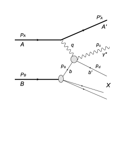
Figure 1: The coherent direct photoproduction processes in which the virtual photon emitted from the whole incident proton A interacts with parton b of another incident proton B via photon-quark Compton scattering, and A remains intact after the photon emitted. A^′ is the scattered proton A, b^′ is the scattered parton b, and X is the sum of residue of B after photon emitted.

For the case of coh.dir (Fig. 1), the invariant cross section of large $p_{T}$ dileptons with $Q^{2}$ distribution is given by

$$\frac{d\sigma^{\textrm{coh.dir}}(p+p\rightarrow p+l^{+}l^{-}+X)}{dM^{2}dQ^{2}}$$

$$= 2\sum_{b}\int dydx_{b}d\hat{t}f_{b/p}(x_{b},\mu_{b}^{2})\frac{d\sigma(p+b\rightarrow p+l^{+}l^{-}+b)}{dM^{2}dQ^{2}dyd\hat{t}},$$

where $x_{b}=p_{b}/P_{B}$ is the parton’s momentum fraction, $f_{b/p}(x_{b},\mu_{b}^{2})$ is the parton distribution function of the proton B Z.Phys.C._53_127 , and the factorized scale is chosen as $\mu_{b}=\sqrt{4p_{T}^{2}}$ Phys.Rev.C._84_044906 . The cross section of the subprocess $p+b\rightarrow p+l^{+}l^{-}+b$ can be written as Phys.Rev.D._79_054007 ; Nucl.Phys.B._904_386

$$\frac{d\sigma(p+b\rightarrow p+l^{+}l^{-}+b)}{dM^{2}dQ^{2}dy}$$ (2)

$$= \frac{\alpha}{3\pi M^{2}}\sqrt{1-\frac{4m_{l}^{2}}{M^{2}}}(1+\frac{2m_{l}^{2}}{M^{2}})\frac{d\sigma(p+b\rightarrow p+\gamma^{*}+b)}{dQ^{2}dy}$$

$$= \frac{\alpha^{2}}{6\pi^{2}M^{2}}\sqrt{1-\frac{4m_{l}^{2}}{M^{2}}}(1+\frac{2m_{l}^{2}}{M^{2}})T_{\mu\nu}\frac{y\rho^{\mu\nu}_{\textrm{coh}}}{Q^{2}}$$

$$\times\frac{d\textrm{P}\textrm{S}_{2}(q+p_{b};p_{c},p_{d})}{2yx_{b}s_{NN}},$$

where $Q^{2}=-q^{2}$, $y=(q\cdot p_{b})/(P_{A}\cdot p_{b})$, $M$ is the invariant mass of dileptons, $m_{l}$ is lepton mass, $T_{\mu\nu}$ is the amplitude of reaction $\gamma^{*}+b\rightarrow\gamma^{*}+b$, $s_{NN}$ is the CM frame energy square of the p-p collision, $d\textrm{PS}_{2}(q+p_{b};p_{c},p_{d})$ is the Lorentz-invariant phase-space measure Nucl.Phys.B._621_337 , the electromagnetic coupling constant is chosen as $\alpha=1/137$, and

$$\rho^{\mu\nu}_{\textrm{coh}} = (-g^{\mu\nu}+\frac{q^{\mu}q^{\nu}}{q^{2}})H_{2}(Q^{2})$$ (3)

$$-\frac{(2P_{A}-q)^{\mu}(2P_{A}-q)^{\nu}}{q^{2}}H_{1}(Q^{2}),$$

is the proton tensor (multiplied by $Q^{-2}$), $H_{1}(Q^{2})$ and $H_{2}(Q^{2})$ are the elastic form factors of proton.

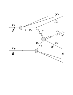
Figure 2: The incoherent direct photoproduction processes in which virtual photon emitted from the parton a of incident proton A interacts with parton b from proton B via the photon-quark interaction, and A is allowed to break up after photon emitted. a denotes the parton of A, $X_{A}$ is the residue of A after photon emitted.

Similarly, the invariant cross section of large $p_{T}$ dileptons produced by incoh.dir (Fig. 2) with $Q^{2}$ distribution has the form

$$\frac{d\sigma^{\textrm{incoh.dir}}(p+p\rightarrow X_{A}+l^{+}l^{-}+X)}{dM^{2}dQ^{2}}$$ (4)

$$= 2\sum_{a,b}\int dydx_{a}dx_{b}d\hat{t}f_{a/p}(x_{a},\mu_{a}^{2})f_{b/p}(x_{b},\mu_{b}^{2})$$

$$\times\frac{d\sigma(a+b\rightarrow a+l^{+}l^{-}+b)}{dM^{2}dQ^{2}dyd\hat{t}},$$

where $x_{a}=p_{a}/P_{A}$ is parton’s momentum fraction, $f_{a/p}(x_{a},\mu_{a}^{2})$ is the parton distribution function of the proton A, $\mu_{a}=\sqrt{4p_{T}^{2}}$. And the cross section of the partonic processes $a+b\rightarrow a+l^{+}l^{-}+b$ reads

$$\frac{d\sigma(a+b\rightarrow a+l^{+}l^{-}+b)}{dM^{2}dQ^{2}dy}$$ (5)

$$= \frac{\alpha}{3\pi M^{2}}\sqrt{1-\frac{4m_{l}^{2}}{M^{2}}}(1+\frac{2m_{l}^{2}}{M^{2}})\frac{d\sigma(a+b\rightarrow a+\gamma^{*}+b)}{dQ^{2}dy}$$

$$= \frac{\alpha^{2}}{6\pi^{2}M^{2}}\sqrt{1-\frac{4m_{l}^{2}}{M^{2}}}(1+\frac{2m_{l}^{2}}{M^{2}})T_{\mu\nu}\frac{e_{a}^{2}y\rho^{\mu\nu}_{\textrm{incoh}}}{Q^{2}}$$

$$\times\frac{d\textrm{P}\textrm{S}_{2}(q+p_{b};p_{c},p_{d})}{2yx_{a}x_{b}s_{NN}},$$

where $e_{a}$ is the charge of massless quark a, $y=(q\cdot p_{b})/(p_{a}\cdot p_{b})$ for the case of incoh.pho, and the massless quark tensor (multiplied by $Q^{-2}$) is

$$\rho^{\mu\nu}_{\textrm{incoh}} = (-g^{\mu\nu}+\frac{q^{\mu}q^{\nu}}{q^{2}})L_{2}(Q^{2})$$ (6)

$$-\frac{(2p_{a}-q)^{\mu}(2p_{a}-q)^{\nu}}{q^{2}}L_{1}(Q^{2}).$$

In Martin-Ryskin method EPJC_74_3040 , the coherent probability (WF) is given by the square of the form factor $F_{1}^{2}(Q^{2})$. Therefore,

$$H_{1}(Q^{2})=H_{2}(Q^{2})=F_{1}^{2}(Q^{2}),$$ (7)

where $F_{1}(Q^{2})$ can be parameterized by the dipole form: $F_{1}(Q^{2})=(1+Q^{2}/0.71\ \textrm{GeV}^{2})^{-2}$.

For the incoherent contribution, the ’remaining’ probability has to be considered for avoiding double counting, and $L_{1}(Q^{2})$, $L_{2}(Q^{2})$ in Eq. (6) have the forms of

$$L_{1}(Q^{2})=L_{2}(Q^{2})=1-F_{1}^{2}(Q^{2}).$$ (8)

By using the linear combinations Phys.Rep._15_181

$$Q^{\mu}=\sqrt{\frac{-q^{2}}{(q\cdot p_{b})^{2}-q^{2}p_{b}^{2}}}(p_{b}-q\frac{q\cdot p_{b}}{q^{2}})^{\mu},$$

$$R^{\mu\nu}=-g^{\mu\nu}+\frac{1}{q\cdot p_{b}}(q^{\mu}p_{b}^{\nu}+q^{\nu}p_{b}^{\mu})-\frac{q^{2}}{(q\cdot p_{b})^{2}}p_{b}^{\mu}p_{b}^{\nu},$$

$\rho^{\mu\nu}$ can be written in the form

$$\rho^{\mu\nu}=\rho^{00}Q^{\mu}Q^{\nu}+\rho^{++}R^{\mu\nu}.$$ (10)

Apparently, $R^{\mu\nu}$ and $Q^{\mu}Q^{\nu}$ are equivalent to transverse and longitudinal polarization Nucl.Phys.B._621_337 : $R^{\mu\nu}=\varepsilon_{T}^{\mu\nu}$, $Q^{\mu}Q^{\nu}=-\varepsilon_{L}^{\mu\nu}$. Thus, the cross section of subprocesses $p+b\rightarrow p+\gamma^{*}+b$ can be expressed as Nucl.Phys.B._904_386

$$\frac{d^{3}\sigma(p+b\rightarrow p+\gamma^{*}+b)}{dydQ^{2}d\hat{t}}$$ (11)

$$= \frac{\alpha}{2\pi}[\frac{y\rho^{++}_{\textrm{coh}}}{Q^{2}}\frac{d\sigma_{T}(\gamma^{*}+b\rightarrow\gamma^{*}+b)}{d\hat{t}}$$

$$+\frac{y\rho^{00}_{\textrm{coh}}}{Q^{2}}\frac{d\sigma_{L}(\gamma^{*}+b\rightarrow\gamma^{*}+b)}{d\hat{t}}],$$

where

$$\rho^{++}_{\textrm{coh}}=F_{1}^{2}(Q^{2})[\frac{1+(1-y)^{2}}{y^{2}}-\frac{2m_{p}^{2}}{Q^{2}}]$$

$$\rho^{00}_{\textrm{coh}}=F_{1}^{2}(Q^{2})\frac{4(1-y)}{y^{2}},$$ (12)

$d\sigma_{T}/d\hat{t}$ and $d\sigma_{L}/d\hat{t}$ represent the transverse and longitudinal cross sections of subprocesses $\gamma^{*}+b\rightarrow\gamma^{*}+b$ respectively,

$$\frac{d\hat{\sigma}_{T}(\gamma^{*}+b\rightarrow\gamma^{*}+b)}{d\hat{t}}$$

$$= \frac{4\pi\alpha^{2}e_{b}^{4}z^{2}}{Q^{4}}[-\frac{\hat{t}}{\hat{s}}-\frac{\hat{s}}{\hat{t}}-M^{2}Q^{2}(\frac{1}{\hat{s}^{2}}+\frac{1}{\hat{t}^{2}})$$

$$+2(Q^{2}-M^{2})\frac{\hat{u}}{\hat{s}\hat{t}}]+\frac{8\pi\alpha^{2}e_{b}^{4}z^{2}}{Q^{4}}\frac{Q^{2}\hat{u}(\hat{t}-M^{2})^{2}}{\hat{t}^{2}(\hat{s}+Q^{2})^{2}},$$

and

$$\frac{d\hat{\sigma}_{L}(\gamma^{*}+b\rightarrow\gamma^{*}+b)}{d\hat{t}}=\frac{8\pi\alpha^{2}e_{b}^{4}z^{2}}{Q^{4}}\frac{Q^{2}\hat{u}(\hat{t}-M^{2})^{2}}{\hat{t}^{2}(\hat{s}+Q^{2})^{2}},$$ (14)

where $z=Q^{2}/(\hat{s}+Q^{2})$, $e_{b}$ is the charge of massless quark b. The Mandelstam variables for subprocesses $\gamma^{*}+b\rightarrow\gamma^{*}+b$ are defined as

$$\hat{s}=(q+p_{b})^{2}=\frac{M^{2}}{z_{q}}+\frac{p_{T}^{2}}{z_{q}(1-z_{q})},$$

$$\hat{t}=(q-p_{c})^{2}=(z_{q}-1)yx_{b}s_{NN},$$

$$\hat{u}=(p_{b}-p_{c})^{2}=M^{2}-z_{q}yx_{b}s_{NN},$$ (15)

where $z_{q}=(p_{c}\cdot P_{B})/(q\cdot P_{B})$ is the inelasticity variable, $p_{T}$ is the transverse momentum in the $\gamma^{*}-b$ CM frame.

In the same way, we can write the cross section of the incoherent subprocesses $a+b\rightarrow a+\gamma^{*}+b$ as

$$\frac{d^{3}\sigma(a+b\rightarrow a+\gamma^{*}+b)}{dydQ^{2}d\hat{t}}$$ (16)

$$= \frac{\alpha}{2\pi}e_{a}^{2}[\frac{y\rho^{++}_{\textrm{incoh}}}{Q^{2}}\frac{d\sigma_{T}(\gamma^{*}+b\rightarrow\gamma^{*}+b)}{d\hat{t}}$$

$$+\frac{y\rho^{00}_{\textrm{incoh}}}{Q^{2}}\frac{d\sigma_{L}(\gamma^{*}+b\rightarrow\gamma^{*}+b)}{d\hat{t}}],$$

where

$$\rho^{++}_{\textrm{incoh}}=(1-F_{1}^{2}(Q^{2}))\frac{1+(1-y)^{2}}{y^{2}}$$

$$\rho^{00}_{\textrm{incoh}}=(1-F_{1}^{2}(Q^{2}))\frac{4(1-y)}{y^{2}},$$ (17)

here we have $\hat{s}=M^{2}/z_{q}+p_{T}^{2}/(z_{q}-z_{q}^{2})$, $\hat{t}=(z_{q}-1)yx_{a}x_{b}s_{NN}$ and $\hat{u}=M^{2}-z_{q}yx_{a}x_{b}s_{NN}$.

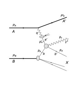
Figure 3: The coherent resolved photoproduction processes in which the incident proton A emits a high energy virtual photon, then the parton $a^{\prime}$ of the resolved photon interacts with the parton b of another incident proton B via the interactions of quark-antiquark annihilation and quark-gluon Compton scattering, and the proton A remains intact after photon emitted.

The resolved photoproduction processes are very important in the research of relativistic heavy ion collisions. The resolved photoproduction processes can also be divided into two categories: coherent resolved photoproduction processes (coh.res) and incoherent resolved photoproduction processes (incoh.res). In the case of coh.res (Fig. 3), the invariant cross section of large $p_{T}$ dileptons with $Q^{2}$ distribution is:

$$\frac{d\sigma^{\textrm{coh.res}}(p+p\rightarrow p+l^{+}l^{-}+X)}{dM^{2}dQ^{2}}$$ (18)

$$= 2\sum_{b}\sum_{a^{\prime}}\int dydx_{b}dz_{a^{\prime}}d\hat{t}f_{b/p}(x_{b},\mu_{b}^{2})f_{\gamma}(z_{a^{\prime}},\mu_{\gamma}^{2})$$

$$\times\frac{\alpha}{2\pi}\frac{y\rho^{++}_{\textrm{coh}}}{Q^{2}}\frac{d\sigma(a^{\prime}+b\rightarrow\gamma^{*}+b)}{dM^{2}d\hat{t}},$$

where $z_{a^{\prime}}$ denotes the parton’s momentum fraction of the resolved photon which are emitted from the proton A, $f_{\gamma}(z_{a^{\prime}},\mu_{\gamma}^{2})$ is the parton distribution function of the resolved photon Phys.Rev.D._60_054019 , $\mu_{\gamma}=\sqrt{4p_{T}^{2}}$. The cross sections of subprocesses $a^{\prime}+b\rightarrow\gamma^{*}+b$ are given by

$$\frac{d\hat{\sigma}}{d\hat{t}}(q\bar{q}\rightarrow\gamma^{*}\gamma)=\frac{2}{3}\frac{\pi\alpha^{2}e_{q}^{4}}{\hat{s}_{\gamma}^{2}}(\frac{\hat{t}_{\gamma}}{\hat{u}_{\gamma}}+\frac{\hat{u}_{\gamma}}{\hat{t}_{\gamma}}+\frac{2M^{2}\hat{s}_{\gamma}}{\hat{u}_{\gamma}\hat{t}_{\gamma}})$$

$$\frac{d\hat{\sigma}}{d\hat{t}}(q\bar{q}\rightarrow\gamma^{*}g)=\frac{8}{9}\frac{\pi\alpha\alpha_{s}e_{q}^{2}}{\hat{s}_{\gamma}^{2}}(\frac{\hat{t}_{\gamma}}{\hat{u}_{\gamma}}+\frac{\hat{u}_{\gamma}}{\hat{t}_{\gamma}}+\frac{2M^{2}\hat{s}_{\gamma}}{\hat{u}_{\gamma}\hat{t}_{\gamma}})$$

$$\frac{d\hat{\sigma}}{d\hat{t}}(qg\rightarrow\gamma^{*}q)=\frac{1}{3}\frac{\pi\alpha\alpha_{s}e_{q}^{2}}{\hat{s}_{\gamma}^{2}}(-\frac{\hat{t}_{\gamma}}{\hat{s}_{\gamma}}-\frac{\hat{s}_{\gamma}}{\hat{t}_{\gamma}}-\frac{2M^{2}\hat{u}_{\gamma}}{\hat{s}_{\gamma}\hat{t}_{\gamma}}).$$

where $\hat{s}_{\gamma}=M^{2}/z_{q}^{\prime}+p_{T}^{2}/(z_{q}^{\prime}-z_{q}^{\prime 2})$, $\hat{t}_{\gamma}=(z_{q}^{\prime}-1)\hat{s}_{\gamma}$ , and $\hat{u}_{\gamma}=M^{2}-z_{q}^{\prime}\hat{s}_{\gamma}$ are the Mandelstam variables for the subprocesses of res.pho, $z_{q}^{\prime}=(p_{c}\cdot p_{b})/(p_{a^{\prime}}\cdot p_{b})$ is the inelasticity variable. The strong coupling constant is taken as the one-loop form Chin.Phys.Lett._32_121202

$$\alpha_{s}=\frac{12\pi}{(33-2n_{f})\ln(\mu^{2}/\Lambda^{2})},$$ (20)

with $n_{f}=3$ and $\Lambda=0.2\ \textrm{GeV}$.

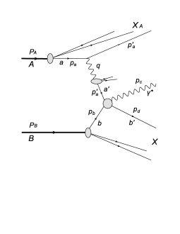
Figure 4: The incoherent resolved photoproduction processes in which the parton $a^{\prime}$ of the resolved photon radiated by parton a of proton A interacts with the parton b from proton B via the quark-antiquark annihilation and quark-gluon Compton scattering, and A is allowed to break up after photon emitted.

The invariant cross section for large $p_{T}$ dileptons produced by incoh.res (Fig. 4) with $Q^{2}$ distribution can be presented as

$$\frac{d\sigma^{\textrm{incoh.res}}(p+p\rightarrow X_{A}+l^{+}l^{-}+X)}{dM^{2}dQ^{2}}$$ (21)

$$= 2\sum_{a,b}\sum_{a^{\prime}}\int dydx_{a}dx_{b}dz_{a^{\prime}}d\hat{t}f_{a/p}(x_{a},\mu_{a}^{2})f_{b/p}(x_{b},\mu_{b}^{2})$$

$$\times f_{\gamma}(z_{a^{\prime}},\mu_{\gamma}^{2})e_{a}^{2}\frac{\alpha}{2\pi}\frac{y\rho^{++}_{\textrm{incoh}}}{Q^{2}}\frac{d\sigma(a^{\prime}+b\rightarrow\gamma^{*}+b)}{dM^{2}d\hat{t}},$$

the cross sections of subprocesses $a^{\prime}+b\rightarrow\gamma^{*}+b$ are discussed in Eq. (II.1).

II.2 The $p_{T}$ distribution of Large $p_{T}$ dileptons production

It is straightforward to obtain the distribution of $p_{T}$ by accordingly reordering and redefining the integration variables in Eq. (II.1). For convenience, the Mandelstam variables in Eq. (II.1) can be written in the form

$$\hat{s} =2\cosh y_{r}M_{T}\sqrt{\cosh^{2}y_{r}M_{T}^{2}-M^{2}}$$ (22)

$$+2\cosh^{2}y_{r}M_{T}^{2}-M^{2},$$

$$\hat{t} =M^{2}-Q^{2}-\sqrt{\hat{s}}M_{T}e^{-y_{r}}+\frac{Q^{2}}{\sqrt{\hat{s}}}M_{T}e^{y_{r}},$$

$$\hat{u} =M^{2}-\sqrt{\hat{s}}M_{T}e^{y_{r}}-\frac{Q^{2}}{\sqrt{\hat{s}}}M_{T}e^{y_{r}},$$

where $y_{r}=\ln(\cot\theta_{c}/2)$ is the rapidity, $\theta_{c}$ is the CM frame scattering angle, $M_{T}=\sqrt{p_{T}^{2}+M^{2}}$ is the dileptons transverse mass. By using the Jacobian determinant, the variables $x_{b}$ and $\hat{t}$ can be transformed into

$$d\hat{t}dx_{b}=|\frac{D(x_{b},\hat{t})}{D(p_{T},y_{r})}|dy_{r}dp_{T}^{2},$$ (23)

where the Jacobian determinant is

$$|\frac{D(x_{b},\hat{t})}{D(p_{T},y_{r})}|$$ (24)

$$= \frac{\cosh y_{r}}{ys_{NN}\sqrt{\cosh^{2}y_{r}M_{T}^{2}-M^{2}}}[M_{T}(2\cosh y_{r}$$

$$+\frac{2\cosh^{2}y_{r}M_{T}^{2}-M^{2}}{M_{T}\sqrt{\cosh^{2}y_{r}M_{T}^{2}-M^{2}}})(M_{T}\sqrt{\hat{s}}-M^{2}e^{y_{r}})$$

$$\times(e^{-2y_{r}}+\frac{Q^{2}}{\hat{s}})+\sinh y_{r}(\hat{s}e^{-y_{r}}+\frac{Q^{2}M^{2}e^{y_{r}}}{\hat{s}})$$

$$\times(2M_{T}+\frac{2\cosh^{2}y_{r}M_{T}^{2}-M^{2}}{\cosh y_{r}\sqrt{\cosh^{2}y_{r}M_{T}^{2}-M^{2}}})].$$

Thus, the invariant cross section of large $p_{T}$ dileptons produced by coh.dir with $p_{T}$ distribution can be expressed as

$$\frac{d\sigma^{\textrm{coh.dir}}_{y_{rc}}(p+p\rightarrow p+l^{+}l^{-}+X)}{dM^{2}dp_{T}^{2}dy_{r}}$$ (25)

$$= 2\sum_{b}\int dQ^{2}dyf_{b/p}(x_{b},\mu_{b}^{2})\frac{\hat{s}}{ys_{NN}p_{T}}(\sqrt{\hat{s}}+\frac{Q^{2}}{\sqrt{\hat{s}}})$$

$$\times\frac{d\sigma(p+b\rightarrow p+l^{+}l^{-}+b)}{dM^{2}dQ^{2}dyd\hat{t}},$$

where $y_{rc}$ represents that the cross section is calculated at $y_{r}=0$, the cross section $d\sigma(p+b\rightarrow p+l^{+}l^{-}+b)/(dM^{2}dQ^{2}dyd\hat{t})$ is discussed in Eq. (2) and Eq. (11).

In the case of incoh.dir, the invariant cross section for large $p_{T}$ dileptons with $p_{T}$ distribution is given by

$$\frac{d\sigma_{y_{rc}}^{\textrm{incoh.dir}}(p+p\rightarrow X_{A}+l^{+}l^{-}+X)}{dM^{2}dp_{T}^{2}dy_{r}}$$

$$= 2\sum_{a,b}\int dQ^{2}dydx_{a}f_{a/p}(x_{a},\mu_{a}^{2})f_{b/p}(x_{b},\mu_{b}^{2})$$

$$\times\frac{\hat{s}}{yx_{a}s_{NN}p_{T}}(\sqrt{\hat{s}}+\frac{Q^{2}}{\sqrt{\hat{s}}})\frac{d\sigma(a+b\rightarrow a+l^{+}l^{-}+b)}{dM^{2}dQ^{2}dyd\hat{t}},$$

the Mandelstam variables are the same as Eq. (22), the cross section $d\sigma(a+b\rightarrow a+l^{+}l^{-}+b)/(dM^{2}dQ^{2}dyd\hat{t})$ is discussed in Eq. (5) and Eq. (16).

For the case of coh.res, the variables $\hat{t}$ and $z_{a^{\prime}}$ can be transformed into

$$d\hat{t}_{\gamma}dz_{a^{\prime}}=|\frac{D(z_{a^{\prime}},\hat{t}_{\gamma})}{D(p_{T},y_{r})}|dy_{r}dp_{T}^{2},$$ (27)

where the Jacobian determinant is

$$|\frac{D(z_{a^{\prime}},\hat{t}_{\gamma})}{D(p_{T},y_{r})}|$$ (28)

$$= \frac{\cosh y_{r}}{yx_{b}s_{NN}\sqrt{\cosh^{2}y_{r}M_{T}^{2}-M^{2}}}[e^{-2y_{r}}M_{T}(2\cosh y_{r}$$

$$+\frac{2\cosh^{2}y_{r}M_{T}^{2}-M^{2}}{M_{T}\sqrt{\cosh^{2}y_{r}M_{T}^{2}-M^{2}}})(M_{T}\sqrt{\hat{s}_{\gamma}}-M^{2}e^{y_{r}})$$

$$+\hat{s}_{\gamma}e^{-y_{r}}\sinh y_{r}(\frac{2\cosh^{2}y_{r}M_{T}^{2}-M^{2}}{\cosh y_{r}\sqrt{\cosh^{2}y_{r}M_{T}^{2}-M^{2}}}$$

$$+2M_{T})],$$

the invariant cross section of large $p_{T}$ dileptons with $p_{T}$ distribution is given by

$$\frac{d\sigma_{y_{rc}}^{\textrm{coh.res.}}(p+p\rightarrow p+l^{+}l^{-}+X)}{dM^{2}dp_{T}^{2}dy_{r}}$$

$$= 2\sum_{b}\sum_{a^{\prime}}\int dQ^{2}dydx_{b}f_{b/p}(x_{b},\mu_{b}^{2})f_{\gamma}(z_{a^{\prime}},\mu_{\gamma}^{2})$$

$$\times\frac{\hat{s}_{\gamma}^{\frac{3}{2}}}{yx_{b}s_{NN}p_{T}}\frac{\alpha}{2\pi}\frac{y\rho^{++}_{\textrm{coh}}}{Q^{2}}\frac{d\sigma(a^{\prime}+b\rightarrow l^{+}l^{-}+b)}{dM^{2}d\hat{t}}.$$

The invariant cross section of large $p_{T}$ dileptons produced by incoh.res with $p_{T}$ distribution can be written as

$$\frac{d\sigma_{y_{rc}}^{\textrm{incoh.res.}}(p+p\rightarrow X_{A}+l^{+}l^{-}+X)}{dM^{2}dp_{T}^{2}dy_{r}}$$ (30)

$$= 2\sum_{a,b}\sum_{a^{\prime}}\int dQ^{2}dydx_{a}dx_{b}f_{a/p}(x_{a},\mu_{a}^{2})f_{b/p}(x_{b},\mu_{b}^{2})$$

$$\times f_{\gamma}(z_{a^{\prime}},\mu_{\gamma}^{2})\frac{\hat{s}^{\frac{3}{2}}_{\gamma}}{yx_{a}x_{b}s_{NN}p_{T}}e_{a}^{2}\frac{\alpha}{2\pi}\frac{y\rho^{++}_{\textrm{incoh}}}{Q^{2}}$$

$$\times\frac{d\sigma(a^{\prime}+b\rightarrow l^{+}l^{-}+b)}{dM^{2}d\hat{t}},$$

where the cross sections of subprocesses $a^{\prime}+b\rightarrow l^{+}l^{-}+b$ are discussed in Eq. (II.1), and the Mandelstam variables for res.pho are the same as Eq. (22) but for $Q^{2}=0$.

II.3 The $Q^{2}$ distribution of Large $p_{T}$ real photon production

The invariant cross sections of large $p_{T}$ real photons can be derived from the invariant cross sections of large $p_{T}$ dileptons produced by photoproduction processes if the invariant mass of dileptons is zero $(M^{2}=0)$. The invariant cross section of large $p_{T}$ real photons produced by coh.dir with $Q^{2}$ distribution satisfy the following form

$$\frac{d\sigma^{\textrm{coh.dir}}(p+p\rightarrow p+\gamma+X)}{dQ^{2}}$$

$$= 2\sum_{b}\int dydx_{b}d\hat{t}f_{b/p}(x_{b},\mu_{b}^{2})\frac{d\sigma(p+b\rightarrow p+\gamma+b)}{dQ^{2}dyd\hat{t}},$$

where the cross section of subprocess $p+b\rightarrow p+\gamma+b$ is similar to Eq. (11), but the transverse and longitudinal cross sections of subprocesses $\gamma^{*}+b\rightarrow\gamma+b$ should be presented as the following forms

$$\frac{d\hat{\sigma}_{T}}{d\hat{t}}(\gamma^{*}+b\rightarrow\gamma+b)$$ (32)

$$= \frac{4\pi\alpha^{2}e_{b}^{4}z^{2}}{Q^{4}}[-\frac{\hat{t}}{\hat{s}}-\frac{\hat{s}}{\hat{t}}+2Q^{2}\frac{\hat{u}}{\hat{s}\hat{t}}]$$

$$+\frac{8\pi\alpha^{2}e_{b}^{4}z^{2}}{Q^{2}}\frac{\hat{u}}{(\hat{s}+Q^{2})^{2}},$$

and

$$\frac{d\hat{\sigma}_{L}}{d\hat{t}}(\gamma^{*}+b\rightarrow\gamma+b)=\frac{8\pi\alpha^{2}e_{b}^{4}z^{2}}{Q^{2}}\frac{\hat{u}}{(\hat{s}+Q^{2})^{2}},$$ (33)

where the Mandelstam variables are $\hat{s}=M^{2}/z_{q}+p_{T}^{2}/(z_{q}-z_{q}^{2})$, $\hat{t}=(z_{q}-1)yx_{b}s_{NN}$, and $\hat{u}=-z_{q}yx_{b}s_{NN}$.

The invariant cross section of large $p_{T}$ real photons produced by incoh.dir with $Q^{2}$ distribution can be expressed as

$$\frac{d\sigma^{\textrm{incoh.dir}}(p+p\rightarrow X_{A}+\gamma+X)}{dQ^{2}}$$ (34)

$$= 2\sum_{a,b}\int dydx_{a}dx_{b}d\hat{t}f_{a/p}(x_{a},\mu_{a}^{2})f_{b/p}(x_{b},\mu_{b}^{2})$$

$$\times\frac{d\sigma(a+b\rightarrow a+\gamma+b)}{dQ^{2}dyd\hat{t}},$$

here we have $\hat{s}=M^{2}/z_{q}+p_{T}^{2}/(z_{q}-z_{q}^{2})$, $\hat{t}=(z_{q}-1)yx_{a}x_{b}s_{NN}$, and $\hat{u}=-z_{q}yx_{a}x_{b}s_{NN}$. The partonic cross sections of $a+b\rightarrow a+\gamma+b$ are analogous with Eq. (16).

In the case of coh.res, the invariant cross section for large $p_{T}$ real photons with $Q^{2}$ distribution has the form

$$\frac{d\sigma^{\textrm{coh.res.}}(p+p\rightarrow p+\gamma+X)}{dQ^{2}}$$ (35)

$$= 2\sum_{b}\sum_{a^{\prime}}\int dydx_{b}dz_{a^{\prime}}d\hat{t}f_{b/p}(x_{b},\mu_{b}^{2})f_{\gamma}(z_{a^{\prime}},\mu_{\gamma}^{2})$$

$$\times\frac{\alpha}{2\pi}\frac{y\rho^{++}_{\textrm{coh}}}{Q^{2}}\frac{d\sigma(a^{\prime}+b\rightarrow\gamma+b)}{d\hat{t}},$$

the cross sections of subprocesses $a^{\prime}+b\rightarrow\gamma+b$ are given by Rev.Mod.Phys._59_465

$$\frac{d\hat{\sigma}}{d\hat{t}}(q\bar{q}\rightarrow\gamma\gamma)=\frac{2}{3}\frac{\pi\alpha^{2}e_{q}^{4}}{\hat{s}_{\gamma}^{2}}(\frac{\hat{t}_{\gamma}}{\hat{u}_{\gamma}}+\frac{\hat{u}_{\gamma}}{\hat{t}_{\gamma}}),$$

$$\frac{d\hat{\sigma}}{d\hat{t}}(q\bar{q}\rightarrow\gamma g)=\frac{8}{9}\frac{\pi\alpha\alpha_{s}e_{q}^{2}}{\hat{s}_{\gamma}^{2}}(\frac{\hat{t}_{\gamma}}{\hat{u}_{\gamma}}+\frac{\hat{u}_{\gamma}}{\hat{t}_{\gamma}}),$$

$$\frac{d\hat{\sigma}}{d\hat{t}}(qg\rightarrow\gamma q)=\frac{1}{3}\frac{\pi\alpha\alpha_{s}e_{q}^{2}}{\hat{s}_{\gamma}^{2}}(-\frac{\hat{t}_{\gamma}}{\hat{s}_{\gamma}}-\frac{\hat{s}_{\gamma}}{\hat{t}_{\gamma}}),$$ (36)

where the Mandelstam variables for the subprocesses of res.pho can be written as $\hat{s}_{\gamma}=M^{2}/z_{q}^{\prime}+p_{T}^{2}/(z_{q}^{\prime}-z_{q}^{\prime 2})$, $\hat{t}_{\gamma}=(z_{q}^{\prime}-1)\hat{s}_{\gamma}$, and $\hat{u}_{\gamma}=-z_{q}^{\prime}\hat{s}_{\gamma}$.

For the case of incoh.res, the invariant cross section of large $p_{T}$ real photons with $Q^{2}$ distribution can be written as

$$\frac{d\sigma^{\textrm{incoh.res.}}(p+p\rightarrow X_{A}+\gamma+X)}{dQ^{2}}$$ (37)

$$= 2\sum_{a,b}\sum_{a^{\prime}}\int dydx_{a}dx_{b}dz_{a^{\prime}}d\hat{t}f_{a/p}(x_{a},\mu_{a}^{2})f_{b/p}(x_{b},\mu_{b}^{2})$$

$$\times f_{\gamma}(z_{a^{\prime}},\mu_{\gamma}^{2})e_{a}^{2}\frac{\alpha}{2\pi}\frac{y\rho^{++}_{\textrm{incoh}}}{Q^{2}}\frac{d\sigma(a^{\prime}+b\rightarrow\gamma+b)}{d\hat{t}},$$

where the cross sections of subprocesses $a^{\prime}+b\rightarrow\gamma+b$ are the same as Eq. (II.3).

II.4 The $p_{T}$ distribution of large $p_{T}$ real photon production

The invariant cross section of large $p_{T}$ real photons produced by coh.dir with $p_{T}$ distribution reads:

$$E\frac{d\sigma_{y_{rc}}^{\textrm{coh.dir}}(p+p\rightarrow p+\gamma+X)}{d^{3}p}$$ (38)

$$= \frac{2}{\pi}\sum_{b}\int dQ^{2}dyf_{b/p}(x_{b},\mu_{b}^{2})\frac{\hat{s}}{ys_{NN}p_{T}}(\sqrt{\hat{s}}+\frac{Q^{2}}{\sqrt{\hat{s}}})$$

$$\times\frac{d\sigma(p+b\rightarrow p+\gamma+b)}{dQ^{2}dyd\hat{t}},$$

the cross sections $d\sigma(p+b\rightarrow p+\gamma+b)/(dQ^{2}dyd\hat{t})$ are discussed in Eq. (11) . And for the case of incoh.dir, the invariant cross section of large $p_{T}$ real photons with $p_{T}$ distribution is:

$$E\frac{d\sigma_{y_{rc}}^{\textrm{incoh.dir}}(p+p\rightarrow X_{A}+\gamma+X)}{d^{3}p}$$

$$= \frac{2}{\pi}\sum_{a,b}\int dQ^{2}dydx_{a}f_{a/p}(x_{a},\mu_{a}^{2})f_{b/p}(x_{b},\mu_{b}^{2})$$

$$\times\frac{\hat{s}}{yx_{a}s_{NN}p_{T}}(\sqrt{\hat{s}}+\frac{Q^{2}}{\sqrt{\hat{s}}})\frac{d\sigma(a+b\rightarrow a+\gamma+b)}{dQ^{2}dyd\hat{t}},$$

the cross sections $d\sigma(a+b\rightarrow a+\gamma+b)/(dQ^{2}dyd\hat{t})$ are discussed in Eq. (16). The Mandelstam variables for dir.pho are the same as Eq. (22) but for $M^{2}=0$.

The invariant cross section of large $p_{T}$ real photons produced by coh.res with $p_{T}$ distribution can be written as:

$$E\frac{d\sigma_{y_{rc}}^{\textrm{coh.res.}}(p+p\rightarrow p+\gamma+X)}{d^{3}p}$$ (40)

$$= \frac{2}{\pi}\sum_{b}\sum_{a^{\prime}}\int dQ^{2}dydx_{b}f_{b/p}(x_{b},\mu_{b}^{2})f_{\gamma}(z_{a^{\prime}},\mu_{\gamma}^{2})$$

$$\times\frac{\hat{s}_{\gamma}^{\frac{3}{2}}}{yx_{b}s_{NN}p_{T}}\frac{\alpha}{2\pi}\frac{y\rho^{++}_{\textrm{coh}}}{Q^{2}}\frac{d\sigma(a^{\prime}+b\rightarrow\gamma+b)}{d\hat{t}},$$

the invariant cross section of large $p_{T}$ real photons produced by incoh.res with $p_{T}$ distribution is given by:

$$E\frac{d\sigma_{y_{rc}}^{\textrm{incoh.res.}}(p+p\rightarrow X_{A}+\gamma+X)}{d^{3}p}$$ (41)

$$= \frac{2}{\pi}\sum_{a,b}\sum_{a^{\prime}}\int dQ^{2}dydx_{a}dx_{b}f_{a/p}(x_{a},\mu_{a}^{2})f_{b/p}(x_{b},\mu_{b}^{2})$$

$$\times f_{\gamma}(z_{a^{\prime}},\mu_{\gamma}^{2})\frac{\hat{s}^{\frac{3}{2}}_{\gamma}}{yx_{a}x_{b}s_{NN}p_{T}}e_{a}^{2}\frac{\alpha}{2\pi}\frac{y\rho^{++}_{\textrm{incoh}}}{Q^{2}}$$

$$\times\frac{d\sigma(a^{\prime}+b\rightarrow\gamma+b)}{d\hat{t}},$$

the cross sections of subprocesses $a^{\prime}+b\rightarrow\gamma+b$ are the same as Eq. (II.3), and the Mandelstam variables for res.pho are the same as Eq. (22), but for $Q^{2}=0$ and $M^{2}=0$.

II.5 The equivalent photons approximation

The idea of EPA approach is treating the field of a fast charged particle as a flux of photons. An essential advantage of EPA is that, when using it, it is sufficient to know the photo-absorption cross section on the mass shell only. Details of its off mass shell behavior are not essential. Thus, the EPA approach, as a useful technique, has been widely used to obtain the various cross sections for charged particles in relativistic heavy ion collisions Phys.Rep._15_181 . Unfortunately, the accuracy of EPA and its applicability range are often neglected Phys.Rev.C._84_044906 ; Phys.Rev.C._91_044908 ; Nucl.Phys.A._865_76 ; Chin.Phys.Lett._29_081301 . The choice of $Q^{2}_{\textrm{max}}\sim\hat{s}$ or $\infty$ is used instead of the significant dynamical cut off $\Lambda^{2}_{\gamma}$ which represents the precision of the EPA approach. However, the exact treatment developed above can be returned to EPA approach by taking $Q^{2}\rightarrow 0$, and the detailed discussion can be found in Ref. Phys.Rep._15_181 . This provides us the powerful comparisons between our results and the ones in the literatures Phys.Rev.C._84_044906 ; Phys.Rev.C._91_044908 . Taking $Q^{2}\rightarrow 0$ is corresponding to that the photon is emitted parallelly from proton or quark, and the variable $y$ becomes the usual momentum fraction ($y=q^{+}/P_{A}^{+}$ for coh.pho and $y=q^{+}/p_{a}^{+}$ for incoh.pho) in the light-front formalism. Since the collinear factorization framework is used for the parton distribution functions, $x_{a}$ and $x_{b}$ are also equal to $p_{a}^{+}/P_{A}^{+}$ and $p_{b}^{+}/P_{B}^{+}$, respectively.

The cross section of subprocess $p+b\rightarrow p+l^{+}l^{-}+b$ with EPA form reads:

$$\frac{d\sigma^{\textrm{coh.pho}}}{dydQ^{2}d\hat{t}} = (\frac{\alpha}{2\pi}\frac{y\rho^{++}_{\textrm{coh}}}{Q^{2}})\frac{d\sigma}{d\hat{t}}$$ (42)

$$= \frac{\alpha}{2\pi}\frac{F_{1}^{2}(Q^{2})}{Q^{2}}[\frac{1+(1-y)^{2}}{y}-y\frac{2m_{p}^{2}}{Q^{2}}]\frac{d\sigma}{d\hat{t}}$$

$$= \frac{df_{\gamma}\shortmid_{\textrm{coh}}(y)}{dQ^{2}}\frac{d\sigma}{d\hat{t}},$$

where $f_{\gamma}\shortmid_{\textrm{coh}}(y)$ is the coherent photon flux which is associated with the whole proton Nucl.Phys.B._904_386 . It should be noted that, since $\sigma_{T}$ and $\sigma_{L}$ are multiplied by the factor $Q^{-2}$, $\sigma_{L}$ and the terms which are proportional to $Q^{2}$ in $\sigma_{T}$ can also provide the non-zero contributions when $Q^{2}\rightarrow 0$, but they are neglected in EPA approach. Actually, the errors from these omissions are so small, and can not cause any noticeable effects.

Another approximate analytic form of the coherent photon flux is developed by Drees and Zeppenfeld (DZ) Phys.Rev.D._39_2536 , which is widely used in the literatures Phys.Rev.C._91_044908 ; Phys.Rev.C._49_1127 ; Nucl.Phys.B._900_431 ; Chin.Phys.Lett._29_081301 . By setting $Q^{2}_{\textrm{max}}\rightarrow\infty$, and neglecting the $m_{p}^{2}$ term in $\rho^{++}_{\textrm{coh}}$, they obtained

$$f_{\gamma}\shortmid_{\textrm{coh}}(y) = \frac{\alpha}{2\pi}\frac{1+(1-y)^{2}}{y}[\ln A$$ (43)

$$-\frac{11}{6}+\frac{3}{A}-\frac{3}{2A^{2}}+\frac{1}{3A^{2}}],$$

where $A=(1+0.71\ \textrm{GeV}^{2}/Q^{2}_{\textrm{min}})$.

For the case of incoh.pho, the cross section of subprocess $a+b\rightarrow a+l^{+}l^{-}+b$ with EPA form reads:

$$\frac{d\sigma^{\textrm{incoh.pho}}}{dydQ^{2}d\hat{t}} = (e_{a}^{2}\frac{\alpha}{2\pi}\frac{y\rho^{++}_{\textrm{incoh}}}{Q^{2}})\frac{d\sigma}{d\hat{t}}$$ (44)

$$= e_{a}^{2}\frac{\alpha}{2\pi}\frac{1-F_{1}^{2}(Q^{2})}{Q^{2}}\frac{1+(1-y)^{2}}{y}\frac{d\sigma}{d\hat{t}}$$

$$= \frac{df_{\gamma}\shortmid_{\textrm{incoh}}(y)}{dQ^{2}}\frac{d\sigma}{d\hat{t}},$$

where $f_{\gamma}\shortmid_{\textrm{incoh}}(y)$ is the incoherent photon flux.

Another form of Eq. (44) , which neglects the $F_{1}^{2}(Q^{2})$ term and takes $Q^{2}_{\textrm{min}}=1\ \textrm{GeV}^{2}$, is

$$f_{\gamma}\shortmid_{\textrm{incoh}}(y) = e_{a}^{2}\frac{\alpha}{2\pi}\frac{1+(1-y)^{2}}{y}\ln\frac{Q^{2}_{\textrm{max}}}{Q^{2}_{\textrm{min}}}.$$ (45)

III NUMERICAL RESULTS

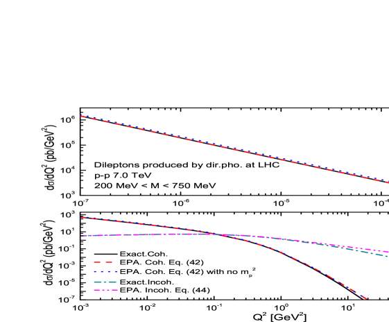
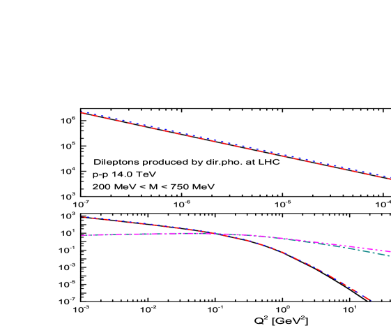
Figure 5: (a) Comparisons of the exact results and EPA ones of dileptons produced by dir.pho for $y_{r}=0$. The solid line (black) represents the exact results of coh.pho, the dash line (red) represents the results of EPA based on the photon flux function Eq. (42), the dot line (blue) represents the results of EPA based on Eq. (42) but without $m_{p}^{2}$ term, the dash-dot line (dark-cyan) represents the exact results of incoh.pho, the dash-dot-dot line (magenta) represents the results of EPA based on the photon flux function of Eq. (44). (b) The same as figure (a) but for p-p collisions at $\sqrt{s_{NN}}=14.0\ \textrm{TeV}$. The solid line (black) coincides with the dash line (red) in small $Q^{2}$ domain. Since the contributions of incoh.pho are so small comparing with coh.pho in the small $Q^{2}$ domain, its results are not plotted in the upper figures.

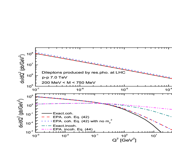
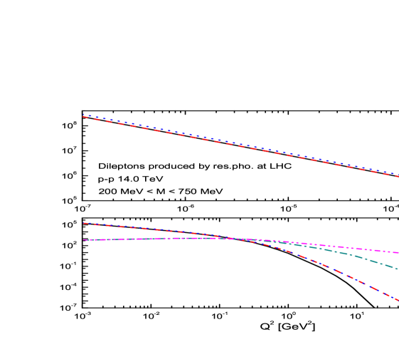
Figure 6: Same as Fig. 5 but for res.pho.

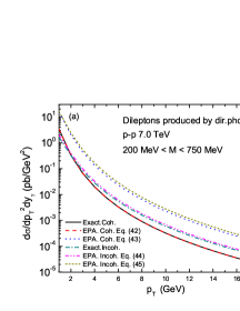
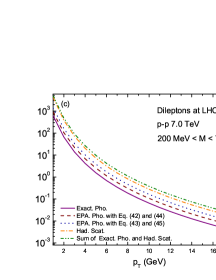
Figure 7: (a) Invariant cross section of dileptons produced by dir.pho. for $y_{r}=0$ in p-p collisions at $\sqrt{s_{NN}}=7.0\ \textrm{TeV}$. (b) Same as (a) but for res.pho. (c) The comparisons between the photoproduction processes results with the ones of hadronic processes, the solid line (purple) represents the exact results of photoproduction processes, the dash line (wine) represents the results of EPA based on Eq. (42) and Eq. (44), the dot line (royal) represents the results of EPA based on Eq. (43) and Eq. (45), the dash-dot line (orange) represents the results of hard scattering of initial partons (had.scat), the dash-dot-dot line (olive) represents the sum of the exact results of photoproduction processes and the ones of had.scat. In Fig. 7 (a) and 7 (b), the solid line (black) coincides with the dash line (red) in the whole $p_{T}$ domain.

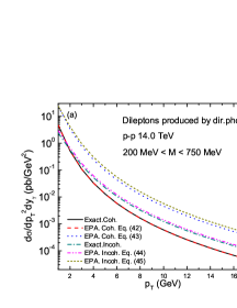
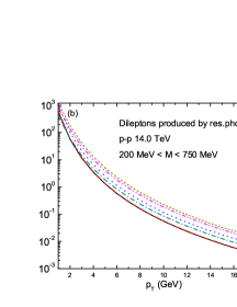
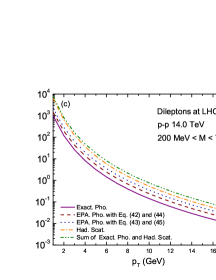
Figure 8: Same as Fig. 7 but for p-p collisions at $\sqrt{s_{NN}}=14\ \textrm{TeV}$.

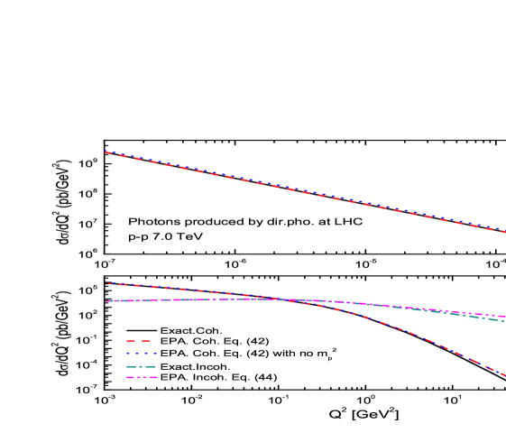
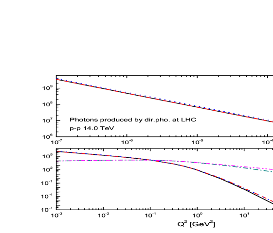
Figure 9: Photons produced by dir.pho. for $y_{r}=0$ in p-p collisions at $\sqrt{s_{NN}}=7.0\ \textrm{TeV}$ (a) and at $\sqrt{s_{NN}}=14.0\ \textrm{TeV}$ (b). The solid line (black) coincides with the dash line (red) in small $Q^{2}$ domain. Since the contributions of incoh.pho are so small comparing with coh.pho in the small $Q^{2}$ domain, its results are not plotted in the upper figures.

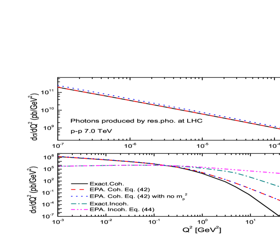
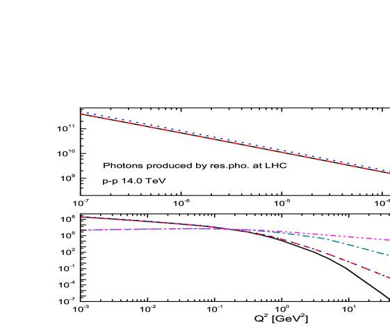
Figure 10: Same as Fig. 9 but for res.pho.

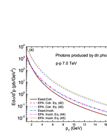
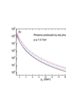
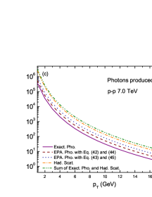
Figure 11: (a) Invariant cross section of photons produced by dir.pho for $y_{r}=0$ in p-p collisions at $\sqrt{s_{NN}}=7.0\ \textrm{TeV}$. (b) Same as (a) but for res.pho. (c) The comparisons between the photoproduction processes results with the ones of hadronic processes. In Fig. 11 (a) and 11 (b), the solid line (black) coincides with the dash line (red) in the whole $p_{T}$ domain.

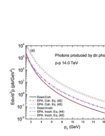
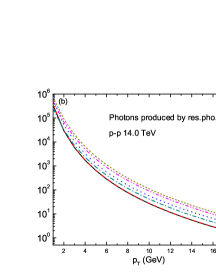
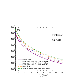
Figure 12: Same as Fig. 11 but for p-p collisions at $\sqrt{s_{NN}}=14\ \textrm{TeV}$

The several theoretical inputs and the bounds of involved variables need to be provided. The mass range of dileptons is chosen as $200\ \textrm{MeV}<M<750\ \textrm{MeV}$, the mass of proton is $m_{p}=0.938\ \textrm{GeV}$ Chin.Phys.C._38_090001 . Since the large $p_{T}$ photoproduction processes are considered (the contribution are mainly from the transverse direction) , the rapidity is set to be $y_{r}=0$ ($\theta_{c}\sim\pi/2$) according to Ref. Phys.Rev.C._84_044906 .

For the $Q^{2}$ distribution, the bounds of integration variables for coh.dir are given by

$$\hat{t}_{\textrm{min}}=(z_{q\ \textrm{min}}-1)yx_{b}s_{NN},$$

$$\hat{t}_{\textrm{max}}=(z_{q\ \textrm{max}}-1)yx_{b}s_{NN},$$

$$x_{b\ \textrm{min}}=\frac{\hat{s}_{\textrm{min}}+Q^{2}}{ys_{NN}},\ x_{b\ \textrm{max}}=1,$$

$$y_{\textrm{min}}=\frac{\hat{s}_{\textrm{min}}+Q^{2}}{s_{NN}},$$

$$y_{\textrm{max}}=\frac{1}{2m_{p}^{2}}\sqrt{4m_{p}^{2}Q^{2}+Q^{4}}+\frac{2m_{p}^{2}-s_{NN}}{2m_{p}^{2}s_{NN}}Q^{2},$$ (46)

where $\hat{s}_{\textrm{min}}=(M_{T\ \textrm{min}}+p_{T\ \textrm{min}})^{2}$, $p_{T}^{2}=\hat{t}(\hat{s}\hat{u}+Q^{2}M^{2})/(\hat{s}+Q^{2})^{2}$ is the square of the transverse momentum for dileptons and

$$z_{q\ \textrm{min}}=\frac{M^{2}+\hat{s}}{2\hat{s}}-\frac{\sqrt{(\hat{s}-M^{2})^{2}-4p_{T\ \textrm{min}}^{2}\hat{s}}}{2\hat{s}}$$

$$z_{q\ \textrm{max}}=\frac{M^{2}+\hat{s}}{2\hat{s}}+\frac{\sqrt{(\hat{s}-M^{2})^{2}-4p_{T\ \textrm{min}}^{2}\hat{s}}}{2\hat{s}}.$$ (47)

The bounds of variables for the incoh.dir are same as Eq. (III), but for $\hat{t}_{\textrm{min}}=(z_{q\ \textrm{min}}-1)yx_{a}x_{b}s_{NN}$, $\hat{t}_{\textrm{max}}=(z_{q\ \textrm{max}}-1)yx_{a}x_{b}s_{NN}$, $x_{b\ \textrm{min}}=(\hat{s}_{\textrm{min}}+Q^{2})/yx_{a}s_{NN}$, $x_{a\ \textrm{min}}=(\hat{s}_{\textrm{min}}+Q^{2})/ys_{NN}$ and $x_{a\ \textrm{max}}=1$.

In the coh.res, the bounds of variables are

$$\hat{t}_{\gamma\ \textrm{min}}=(z_{q\ \textrm{min}}^{\prime}-1)z_{a}yx_{b}s_{NN},$$

$$\hat{t}_{\gamma\ \textrm{max}}=(z_{q\ \textrm{max}}^{\prime}-1)z_{a}yx_{b}s_{NN},$$

$$z_{a\ \textrm{min}}=\frac{\hat{s}_{\gamma\ \textrm{min}}}{yx_{b}s_{NN}},\ z_{a\ \textrm{max}}=1,$$

$$x_{b\ \textrm{min}}=\frac{\hat{s}_{\gamma\ \textrm{min}}}{z_{a\ \textrm{max}}ys_{NN}},\ x_{b\ \textrm{max}}=1,$$

$$y_{\textrm{min}}=\frac{\hat{s}_{\gamma\ \textrm{min}}}{z_{a\ \textrm{max}}s_{NN}},$$ (48)

$y_{\textrm{max}}$ is same as Eq. (III), where $\hat{s}_{\gamma\ \textrm{min}}=(M_{T\ \textrm{min}}+p_{T\ \textrm{min}})^{2}$, $p_{T}^{2}=\hat{t}\hat{u}/\hat{s}$ and

$$z_{q\ \textrm{min}}^{\prime}=\frac{M^{2}+\hat{s}_{\gamma}}{2\hat{s}_{\gamma}}-\frac{\sqrt{(\hat{s}_{\gamma}-M^{2})^{2}-4p_{T\ \textrm{min}}^{2}\hat{s}_{\gamma}}}{2\hat{s}_{\gamma}}$$

$$z_{q\ \textrm{max}}^{\prime}=\frac{M^{2}+\hat{s}_{\gamma}}{2\hat{s}_{\gamma}}+\frac{\sqrt{(\hat{s}_{\gamma}-M^{2})^{2}-4p_{T\ \textrm{min}}^{2}\hat{s}_{\gamma}}}{2\hat{s}_{\gamma}}.$$

The bounds of variables for the incoh.res are same as Eq. (III) but for $\hat{t}_{\gamma\ \textrm{min}}=(z_{q\ \textrm{min}}^{\prime}-1)z_{a}yx_{a}x_{b}s_{NN}$, $\hat{t}_{\gamma\ \textrm{max}}=(z_{q\ \textrm{max}}^{\prime}-1)z_{a}yx_{a}x_{b}s_{NN}$, $z_{a\ \textrm{min}}=\hat{s}_{\gamma\ \textrm{min}}/(yx_{a}x_{b}s_{NN})$, $x_{b\ \textrm{min}}=\hat{s}_{\gamma\ \textrm{min}}/(z_{a\ \textrm{max}}yx_{a}s_{NN})$, $x_{a\ \textrm{min}}=\hat{s}_{\gamma\ \textrm{min}}/(z_{a\ \textrm{max}}ys_{NN})$ and $x_{a\ \textrm{max}}=1$.

For the $p_{T}$ distribution, the bounds of $x_{a}$, $x_{b}$ and $y$ are same as $Q^{2}$ distribution, but for $z_{a\ \textrm{max}}=1/(1+Q^{2}/(4p_{T}^{2}))$ Phys.Rev.D_29_852 ; Phys.Rev.D._51_3320 , the bounds of $Q^{2}$ are $Q^{2}_{\textrm{min}|\textrm{coh.dir}}=x_{1}^{2}m_{p}^{2}/(1-x_{1})$, $x_{1}=\hat{s}/s_{NN}$, $Q^{2}_{\textrm{min}|\textrm{incoh.dir}}=0$, $Q^{2}_{\textrm{min}|\textrm{coh.res}}=Q^{2}_{\textrm{min}|\textrm{incoh.res}}=0.01\ \textrm{GeV}^{2}$ EPJC_10_313 , and $Q^{2}_{\textrm{max}}=4p_{T}^{2}$ is used for the exact calculations and the EPA ones Eq. (42) and Eq. (44).

In Fig. 5 and 6, the $Q^{2}$ distribution of dileptons produced by photoproduction processes in p-p collisions at LHC energies are plotted. The contribution of exact treatment are compared with the EPA ones. For the case of coh.dir, the results of EPA share the same trend with the exact one in the small $Q^{2}$ region, since EPA is obtained by setting the photon virtuality $Q^{2}\rightarrow 0$ and neglecting the longitudinal photon contributions. Considering that the coherent photon flux function with the DZ form Eq. (43) is obtained by neglecting the $m_{p}^{2}$ term, the EPA result Eq. (42) with no $m_{p}^{2}$ term is also presented for researching the $Q^{2}$ dependence behaviour and the validity of Eq. (43). It can be seen that, the EPA result with no $m_{p}^{2}$ term is greater than the result of Eq. (42) at small $Q^{2}$ domain, but they become consistent with increasing $Q^{2}$, since the $m_{p}^{2}$ term is inversely proportional to $Q^{2}$. The exact result is in agreement with the EPA results Eq. (42) in small $Q^{2}$ region, and is less than the EPA ones when $Q^{2}>10\ \textrm{GeV}^{2}$. The case of coh.res is similar to coh.dir, but the differences between the exact results and the EPA ones are much more evident in large $Q^{2}$ domain. Therefore, the EPA approach is only suitable in the small $Q^{2}$ domain, and can be used as a good approximation for coh.pho, since the small $Q^{2}$ domain give the main contribution which agree with the statements of Martin and Ryskin in Ref. EPJC_74_3040 , and of Budnev and Ginzburg in Ref. Phys.Rep._15_181 . And the errors from the omission of $m_{p}^{2}$ term in Eq. (42) and the option of $Q^{2}_{\textrm{max}}\sim\hat{s}\ or\ \infty$ in Eq. (42) and Eq. (43) can not be neglected.

For the case of incoh.dir, the exact result and the EPA ones are almost same and can be neglected comparing with coh.dir when $Q^{2}<0.01\ \textrm{GeV}^{2}$, but the differences among them are evident when $Q^{2}>0.1\ \textrm{GeV}^{2}$. Besides, the incoh.dir contribution is comparable with the coh.dir contribution when $Q^{2}>0.01\ \textrm{GeV}^{2}$, and becomes much larger when $Q^{2}>0.1\ \textrm{GeV}^{2}$. The case of incoh.res is similar to incoh.dir, but the differences between the exact results and the EPA ones are more prominent in large $Q^{2}$ domain. It should be emphasized that, if the Martin-Ryskin method is not considered, the incoh.pho contribution will always much larger than the coh.pho one in the whole $Q^{2}$ region and is divergent at very small $Q^{2}$ domain ($Q^{2}\rightarrow 0$). This is a unphysical result. Comparing with the Martin-Ryskin method which avoid this unphysical large value of incoh.pho naturally, the physical interpretation is not clear in literatures Nucl.Phys.B._900_431 ; Phys.Rev.C._92_054907 ; Phys.Rev.C._84_044906 ; Phys.Rev.C._91_044908 ; Chin.Phys.Lett._29_081301 which calculated the incoh.pho contribution by using the artificial cutoff $Q^{2}>1\ \textrm{GeV}^{2}$. Therefore, the EPA approach is not a effective approximation for incoh.pho, since the incoh.pho contribution are mainly from the large $Q^{2}$ domain where the errors are obvious, and the results in these works are not accurate enough.

The $p_{T}$ distribution of dileptons produced by photoproduction processes in p-p collisions at LHC energies are illustrated in Fig. 7 and 8. For the case of coh.dir, the exact result nicely agrees with EPA one Eq. (42) in the whole $p_{T}$ region. However, the result of Eq. (43) is much larger than the results of exact treatment and Eq. (42), since Eq. (43) is obtained by neglecting the $m_{p}^{2}$ term in Eq. (42), and setting $Q^{2}_{\textrm{max}}=\infty$ which will cause obvious errors. It can be seen that, the contribution of res.pho is about two orders of magnitude larger than the dir.pho, thus the contribution of large $p_{T}$ dileptons produced by photoproduction processes is mainly from res.pho. The case of coh.res is similar to coh.dir, the errors from Eq. (43) is also prominent. Therefore, the choice of $Q^{2}_{\textrm{max}}$ is crucial to the accuracy of EPA. Eq. (42) with $Q^{2}_{\textrm{max}}=4p_{T}^{2}$ is a good choice for calculating coh.pho. However, choosing $Q^{2}\sim\infty$ will cause the large fictitious contribution from the large $Q^{2}$ domain (it can be found in the figures which show the $Q^{2}$ dependence behaviour), which agree with the statements in Ref. Phys.Rep._15_181 . For the practical use of EPA, except considering the kinematically allowed $Q^{2}$-change region, one should also elucidate whether there is a dynamical cut off $\Lambda^{2}_{\gamma}$, and estimate it. However, the definite values of the $\Lambda_{\gamma}^{2}$ for different processes are essentially different, and still need further studies.

For the case of incoh.dir, the EPA results are greater than the exact one in the whole $p_{T}$ region, but the difference between the EPA result Eq. (45) and the exact one is much more evident, since the $Q_{\textrm{max}}^{2}$ is set be $\hat{s}/4$ in Eq. (45), which include the errors from the large $Q^{2}$ domain. The incoh.res is similar to incoh.dir, the differences between the exact result and the EPA ones are prominent in the whole $p_{T}$ region. Thus, the EPA approach can not be used in incoh.pho and the effects of the inapplicability of EPA for incoh.pho are significant. In Fig. 7 (c) and 8 (c), the comparisons between the photoproduction processes and the one of initial partons hard scattering are presented. It can be seen that the corrections from the exact results of photoproduction processes to had.scat are non-negligible, especially in the large $p_{T}$ domain. However, the differences between the EPA results and the exact one are evident. The EPA results will give the large fictitious correction to the production of dileptons and photons, especially for the EPA result of Eq. (43) and Eq. (45). Thus the statements are not accurate in Ref. Phys.Rev.C._84_044906 ; Phys.Rev.C._91_044908 , in which the incoh.pho of dileptons and photons was calculated by using the EPA approach Eq. (45) with $Q^{2}_{\textrm{max}}=\hat{s}/4$ and $Q^{2}_{\textrm{min}}=1\ \textrm{GeV}^{2}$, and the coh.pho was calculated by using the photon flux function with the DZ form Eq. (43).

Fig. 9 and 10 present the $Q^{2}$ distribution of real photons produced by photoproduction processes in p-p collision at LHC energies. It is shown that the differences among the exact result and EPA ones are more obvious in the large $Q^{2}$ region. The $p_{T}$ distribution of real photons produced by photoproduction processes in p-p collision at LHC energies can be found in Fig. 11 and Fig. 12. The results are similar to the case of dileptons in Fig. 7 and 8, but the inapplicability of EPA for incoh.pho and the errors from the option of $Q^{2}_{\textrm{max}}\sim\infty$ and $Q^{2}_{\textrm{max}}=\hat{s}/4$ are more obvious. We also compare our results of real photons to Ref. Phys.Rev.C._84_044906 ; Phys.Rev.C._91_044908 , the inaccuracy of EPA is more evident. Therefore, the EPA can be used for coh.pho with the suitable choice of $Q^{2}_{\textrm{max}}$. And for incoh.pho, EPA is not an effective treatment, since it dominates the large $Q^{2}$ region where the errors are obvious. Thus, the exact treatment is needed to deal accurately with the photoproduction of dileptons and photons.

IV SUMMARY AND CONCLUSIONS

We have investigated the production of large $p_{T}$ dileptons and photons induced by photoproduction processes in p-p collisions at LHC energies, and presented the distributions of $Q^{2}$ and $p_{T}$. The exact treatment, which returns to the EPA approach in the limit $Q^{2}\rightarrow 0$, is developed for calculations. The coherent and incoherent photon emission processes are considered simultaneously and the Martin-Ryskin method is used for avoiding the double counting. The comparisons between the exact results and EPA ones are presented for discussing the applicability range of EPA and its accuracy. The numerical results indicate that, the EPA approach is only a good approximation in the small $Q^{2}$ region and can be used for coh.pho with the suitable option of $Q^{2}_{\textrm{max}}$. For incoh.pho, EPA is not an effective approximation, since the incoh.pho dominate the large $Q^{2}$ region where the errors are obvious. The photon flux function Eq. (43) developed by Drees and Zeppenfeld and Eq. (45) with $Q^{2}_{\textrm{max}}=\hat{s}/4$ are widely used in the literatures Nucl.Phys.B._904_386 ; Phys.Rev.C._92_054907 ; Chin.Phys.Lett._29_081301 ; Nucl.Phys.A._865_76 ; Phys.Rev.C._84_044906 ; Phys.Rev.C._91_044908 , and the the imprecise statements were given. Therefore, EPA can not provide accurate enough results for the photoproduction of large-$p_{T}$ dileptons and photons in p-p collision, and the exact treatment should be considered.

References

- (1) E. Fermi, Z. Phys. 29, 315 (1924).
- (2) K. F. V. Weizsäcker, Z. Phys. 88, 612 (1934).
- (3) E. J. Williams, Phys. Rev. 45, 729 (1934).
- (4) L.D. Landau and E.M. Lifshitz, Sov. Phys. 6, 244 (1934).
- (5) G. Nordheim et al., Phys. Rev. 51, 1037 (1937).
- (6) R. H. Dalitz and D. R. Yennie, Phys. Rev. 105, 1598 (1957).
- (7) I. Ya. Pomeranchuk and I. M. Shmushkevich, Nucl. Phys. 23, 1295 (1961).
- (8) R. B. Curtis, Phys. Rev. 104, 211 (1956).
- (9) J. Q. Zhu, Z. L. Ma, C. Y. Shi, and Y. D. Li, Phys. Rev. C 92, 054907 (2015).
- (10) Y. P. Fu and Y. D. Li, Nucl. Phys. A865, 76 (2011).
- (11) Y. P. Fu and Y. D. Li, Phys. Rev. C 84, 044906 (2011).
- (12) G. M. Yu and Y. D. Li, Phys. Rev. C 91, 044908 (2015).
- (13) J. Q. Zhu and Y. D. Li, Chin. Phys. Lett. 29, 081301 (2012).
- (14) J. Q. Zhu, Z. L. Ma, C. Y. Shi and Y.D. Li, Nucl. Phys. B900, 431 (2015).
- (15) A. J. Baltz, et al. Phys. Rep. 458, 1 (2008).
- (16) C.J. Brown and D.H. Lyth, Nuel. Phys. B53, 323 (1973).
- (17) V. M. Budnev, I. F. Ginzburg, G. V. Meledin, and V. G. Serbo, Phys. Rep. 15, 181 (1975).
- (18) S. J. Brodsky, T. Kinoshita, and H. Terazawa, Phys. Rev. D 4, 1532 (1971); H. Terazawa, Rev. Mod. Phys. 45, 615 (1973).
- (19) M. Drees and D. Zeppenfeld, Phys. Rev. D 39, 2536 (1989); B. A. Kniehl, Phys. Lett. B 254, 267 (1991).
- (20) M. Drees, J. Ellis and D. Zeppenfeld, Phys. Lett. B 223, 454 (1989).
- (21) S. Frixione, M. L. Mangano, P. Nason, and G. Ridolfi, Phys. Lett. B 319, 339 (1993).
- (22) R. Nisius, Phys. Rep. 332, 165 (2000).
- (23) Y. D. Li and L. S. Liu, Phys. Lett. B 377, 177 (1996).
- (24) M. Krawczyk, A. Zembrzuski, and M. Staszel, Phys. Rep. 345, 265 (2001).
- (25) J. M. Butterworth, J. R. Forshaw, and M. H. Seymour, Z. Phys. C 72, 637 (1996).
- (26) J. F. Owens, Rev. Mod. Phys. 59, 465 (1987).
- (27) G. Baur, K. Hencken, and D. Trautmann, J. Phys. G. 24, 1657 (1998).
- (28) J. Q. Zhu and Y. D. Li, Nucl. Phys. B904, 386 (2016).
- (29) A. D. Martin and M. G. Ryskin, Eur. Phys. J. C 74, 3040 (2014).
- (30) B. A. Kniehl and L. Zwirner, Nucl. Phys. B621, 337 (2002).
- (31) M. Glück, E. Reya, and A. Vogt, Z. Phys. C 53, 127 (1992).
- (32) Z. B. Kang, J. W. Qiu and W. Vogelsang, Phys. Rev. D 79, 054007 (2009); R. D. Field, Applications of perturbative QCD (Addison-Wesley Publishing Company, Reading, MA, 1989).
- (33) M. Glück, E. Reya, and I. Schienbein, Phys. Rev. D 60, 054019 (1999).
- (34) Z. L. Ma, J. Q. Zhu, C. Y. Shi, and Y. D. Li, Chin. Phys. Lett. 32, 121202 (2015).
- (35) N. Baron and G. Baur, Phys. Rev. C 49, 1127 (1994); M. Drees, R. M. Godbole, M. Nowakowski and S. D. Rindani, Phys. Rev. D 50, 2335 (1994).
- (36) K. A. Olive, et al., Particle Data group, Chin. Phys. C 38, 090001 (2014).
- (37) G. Rossi, Phys. Rev. D 29, 852 (1984).
- (38) M. Glück, E. Reya, and M. Stratmann, Phys. Rev. D 51, 3220 (1995).
- (39) M. Glück, E. Reya, and I. Schienbein, Eur. Phys. J. C 10, 313 (1999).