A Robust Interferometry Against Imperfections Base on Weak Value Amplification

Abstract

The optical interferometry has been widely used in various high precision applications. Usually, the minimum precision of an interferometry is limited by various technique noises in practice. To suppress such kind of noises, we propose a novel scheme, which combines the weak measurement with the standard interferometry. The proposed scheme dramatically outperforms the standard interferometry in the signal noise ratio and the robustness against noises caused by the optical elements’ reflections and the offset fluctuation between two paths. A proof-of-principle experiment is demonstrated to validate the amplification theory.

I Introduction

The optical interferometry has been widely used in science and industry fields, such as physicsLIGO2016 , astronomyAstro2003 , engineeringBiegen1988 , applied scienceatom1997 , biologyDIC1981 and medicineHuang1991 . In all of these applications, an important issue is to detect the length difference or the phase difference between different paths. Making use of the obtained differences, one may achieve a highest precision length measurementLIGO2016 . Theoretically, the minimum measurable length difference is limited by the shot noise limitGiovannetti2011 , which is inversely proportional to the square root of the input intensity and the number of measurement events. While in practice, the technical noises may cause uncertainty that usually much higher than the theoretical limit. Hence to suppress the practical technical noises has become an important issue in applications of the interferometry.

Aiming to the high precision detection, a technique called the weak value amplification(WVA)Aharonov1988 ; Hosten2008 ; Dixon2009 ; Viza2013 ; Xu2013 ; Fang2016 ; OAM2014 ; Hu2017 can suppress the technique noises to increase the signal noise ratio(SNR). This has been demonstrated in theoriesJordan2014 ; Brunner2010 ; Li2011 and experimentsXu2013 ; Fang2016 . Physically, such kind of suppression can be achieved by amplifying the signal at the cost of decreasing the probability of detection. Due to the amplification, small changes beyond the detector resolution can even be detected Hosten2008 ; Dixon2009 .

In this paper, we propose a scheme named weak value amplified interferometry(WVAI) which merges the WVA and the standard interferometry(SI) together. By applying the WVA technique, this scheme amplifies the phase difference before detection in an interferometer. The amplification provides the robustness against technique noises. Based on an optical Mach-Zehnder interferometer, the performance of the proposed scheme is investigated. Then the influences of two kinds of technique noises, which are respectively caused by the reflections of the optical elements and the fluctuations of the phase offset, are studied. The results show that the WVAI scheme outperforms the SI in the SNR and in the the technique noise suppression. In addition, a proof-of-principle experiment is demonstrated to verify the phase amplification effect of the WVAI scheme.

This paper is organized as follows: In Sec. II we present a new interferometry scheme named WVAI. Then the influences of two typical technique noises, which are respectively caused by the reflections of the optical elements and the fluctuations of the offset between two paths, are investigated in Sec. III. In Sec. IV a proof-of-principle experiment is demonstrated and analyzed. Finally, Sec.V concludes this paper.

II Scheme Description

Before presenting the proposed scheme, let’s consider an optical Mach-Zehnder interferometer to exemplify the standard interferometry. Displayed in Fig. 1(a), a monochromatic laser beam is split into two paths by the BS1 with 50/50 splitting ratio. In the lower path, $e^{-i\theta}$ stands for the phase difference between two paths. While in the upper path, a controllable phase $\phi$ is introduced as an offset phase delay. The two beams in the two paths interfere after they recombining by the BS2. Then one can collect the intensity of the interference by a detector, which is

$$I_{D_{I}}(\theta) =I_{in}|\frac{e^{-i\phi}+e^{-i\theta}}{\sqrt{2}}|^{2}$$ (1)

$$=\frac{I_{in}}{4}[1+\cos(\phi-\theta)],$$

where $I_{in}$ is the input light intensity. The subscript ”I” represents the SI scheme.

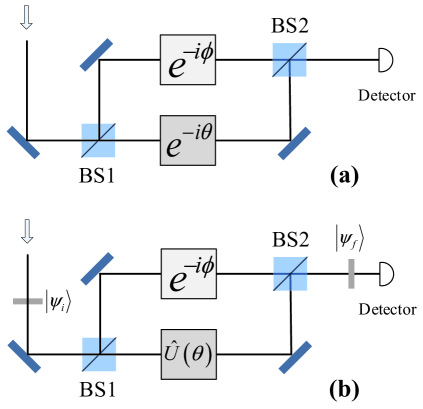
Figure 1: (Color online). The schematic diagram of the SI(a) and the WVAI(b) based on an optical Mach-Zehnder interferometer.

With a little modification, one can combine the interferometer with the WVA technique. As indicated in Fig.1(b), two linear polarizers are inserted before the BS1 and after the BS2, respectively. These polarizers are used to selected the system in the preselected state $|\psi_{i}\rangle=1/\sqrt{2}(|H\rangle+|V\rangle)$ and in the postselected state $|\psi_{f}\rangle=\cos\alpha|H\rangle+\sin\alpha|V\rangle)$, respectively. Note that H and V stands for horizontal and vertical polarized direction respectively. The phase difference $e^{-i\theta}$ is replaced with a unitary operation $\hat{U}(\theta)=e^{-i\theta\hat{A}}$, where $A\equiv|H\rangle\langle H|-|V\rangle\langle V|$. Then one obtains a WVAI scheme based on an optical Mach-Zehender interferometer. Other types of interferometer, such as Michelson, Sagnac and atom interferometer, etc., will be straightforward.

The output state of the modified interferometer is expressed as

$$|\Psi_{out}\rangle=\langle\psi_{f}|\frac{e^{-i\phi}+\hat{U}(\theta)}{\sqrt{2}}|\psi_{i}\rangle|\phi(p)\rangle,$$ (2)

where $|\phi(p)\rangle$ is the input laser state, $p$ stands for the momentum. When $\alpha=-\pi/4+\epsilon,|\theta/\epsilon|\ll 1$, the output state could be written in its first-order-approximation

$$|\Psi_{out}\rangle\approx\langle\psi_{f}|\psi_{i}\rangle\frac{e^{-i\phi}+e^{-iA_{w}\theta}}{\sqrt{2}}|\phi(p)\rangle,$$ (3)

where

$$A_{w}=\frac{\langle\psi_{f}|\hat{A}|\psi_{i}\rangle}{\langle\psi_{f}|\psi_{i}\rangle}=\frac{\cos\alpha-\sin\alpha}{\cos\alpha+\sin\alpha}=\cot\epsilon.$$ (4)

The detector collects the light selected by $|\psi_{f}\rangle$. The detected intensity is given by

$$I_{D_{A}}(\theta) \approx I_{in}\langle\psi_{f}|\psi_{i}\rangle^{2}|\frac{e^{-i\phi}+e^{-iA_{w}\theta}}{\sqrt{2}}|^{2}$$ (5)

$$=\frac{I_{in}}{4A_{w}^{2}}[1+\cos(\phi-A_{w}\theta)],$$

where the subscript ”A” indicates the proposed scheme. Because of the postselection, the orthogonal polarized parts are neglected. The successful selected probability is $1/A_{w}^{2}$.

In the following, we evaluate the performance of the proposed scheme with two features. The first one is the output intensity difference between no phase delay input and $\theta(\theta>0)$ input, which is

$$\Delta I_{D}=I_{D}(\theta)-I_{D}(0).$$

This difference can be obtained by differential detectionDiff or phase and amplitude modulationFOG . The second one is the intensity contrast ratio, i.e. $I(\theta)/I(0)$, which represents the ratio of the intensity variation (detected signal) induced by the phase delayQiu2017 .

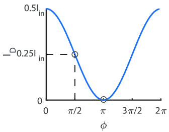
Figure 2: (Color online). The output intensity $I_{D}$ of different offsets $\phi$ without phase delay input in the standard interferometry.

Fig.2 shows the output intensity of different offsets without phase delay input in the SI. Based on the WVAI scheme one may get a similar curve with an attenuation of $1/A_{w}^{2}$ in the amplitude. Typically, the offset $\phi$ is set at two phase values, i.e. $\pi/2$ and $\pi$, for the highest sensitivity and the weak signal detection, respectively.

When $\phi=\pi$, the interferometer has total destructive interference. Since it’s easier to detect a brightening of nothing than to detect a dimming of a bright light, this offset is usually set for weak signal detection like gravitational waves detection. Omitting the technique noise, $\Delta I_{D}$ is equal to the detected intensity in both the WVAI and the SI scheme, which can be written in the first-order approximation respectively

$$\Delta I_{D_{A}}=I_{D_{A}}\approx I_{in}\theta^{2}/8,$$ (6)

$$\Delta I_{D_{I}}=I_{D_{I}}\approx I_{in}\theta^{2}/8.$$

Explicitly, the output intensity difference is proportional to the quadratic term of $\theta$. Although $\theta$ has been amplified, the WVAI scheme detects the same intensity as the SI does. This degradation is blamed to discarding light in the postselection. Furthermore, both methods obtain infinite intensity contrast ratios.

When $\phi=\pi/2$, this offset leads to a maximum sensitivity of the interferometer. It can be found in Fig.2, the curve has the maximum gradient with $\phi=\pi/2$. In this situation,

$$\Delta I_{D_{A}}=\frac{0.25I_{in}\sin(A_{w}\theta)}{A_{w}^{2}}\approx\frac{0.25I_{in}\theta}{A_{w}},$$ (7)

$$\Delta I_{D_{I}}=0.25I_{in}\sin\theta\approx 0.25I_{in}\theta.$$

Obviously, $\Delta I_{D_{A}}$ is $1/A_{w}$ of $\Delta I_{D_{I}}$ which is caused by the low postselection’s probability. However, due to the amplified phase, the WVAI outperforms than the SI on the intensity contrast ratio. As shown in Fig.3, the intensity contrast ratio rises along with the increasing of $A_{w}$.

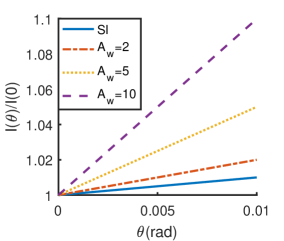
Figure 3: (Color online). The intensity contrast ratio with the offset $\phi=\pi/2$ of the SI(solid line), $A_{w}=2$(dash-dotted line), $A_{w}=5$(dotted line), $A_{w}=10$(dashed line).

Clearly, when the phase offset is set at $\phi=\pi$, the WVAI scheme and the SI scheme have the same output intensities, which means that they have the same detection uncertainty. Both scheme get infinite intensity contrast ratios. While with the offset $\pi/2$, the WVAI scheme obtain a higher intensity contrast ratio at the expense of losing the output intensity. However, if the power-recyclepowerrecycle2016 is taken into consideration, all the light will go through the postselection without attenuation. One may gain a $A_{w}^{2}$ times magnificence of the output intensity, which is

$$\ I_{D_{A}}(\theta)\approx\frac{I_{in}}{4}[1+\cos(\phi-A_{w}\theta)].$$ (8)

The amplified phase will boost the performance with any $\phi$. With balanced differential detectors, a $\pi/2$ offset will lead to a $A_{w}$ times enhancement of sensitivity than SI.

III Imperfection analysis

In this section, we discuss two typical kinds of technique noises as examples to demonstrate the robustness of the proposed scheme against the noises. These noises are caused by the reflections of imperfect optical elements and the fluctuation of the offset $\phi$, respectively.

III.1 Reflection of imperfect optical elements

Practically, all optical elements’ transmission ratio can’t be 1. The reflected light will interfere with the output light field. For example, in the proposed scheme depicted in the Fig.1, the imperfections of BS1, BS2, and all the mirrors could cause this problem. The reflected light field before postselection can be written as $E_{in}\eta_{n}e^{i\delta_{n}}$, where the subscript $n$ denotes the number of the optical elements, $E_{in}$, $\eta_{n}$ and $\delta_{n}$ are the input light field, the square root of the reflectivity, and the relative phase of corresponding elements, respectively. Generally, one has the following expression

$$\eta e^{i\delta}=\sum\nolimits_{n=1}^{N}\eta_{n}e^{i\delta_{n}},$$

where $N$ is the total number of optical elements, $\eta=\sqrt{\sum\nolimits_{n=1}^{N}\eta_{n}^{2}}$, and $\tan\delta=\frac{\sum\nolimits_{n=1}^{N}\sin\delta_{n}}{\sum\nolimits_{n=1}^{N}\cos\delta_{n}}$. Commonly, $\eta\ll 1$ and $\delta$ can be any value from $-\pi$ to $\pi$. Then the output intensity described by Eq. (5) becomes

$$I_{D_{A}}(\theta) \approx I_{in}\langle\psi_{f}|\psi_{i}\rangle^{2}|e^{-i\phi}+e^{-iAw\theta}+\sum\nolimits_{n=1}^{N}\eta_{n}e^{i\delta_{n}}|^{2}$$ (9)

$$=\frac{I_{in}}{4A_{w}^{2}}\{1+\frac{\eta^{2}}{2}+\cos(\phi-A_{w}\theta)$$

$$+\eta[\cos(\phi+\delta)+\cos(A_{w}\theta+\delta)]\}.$$

When $\phi=\pi$, according to the Taylor expansion to the second order in Eq. (9) one acquires

$$\Delta I_{D_{A}}(\theta)\approx(S_{1A}+\sigma_{1A}^{(n)})I_{in},$$

where

$$\left\{\begin{aligned} &S_{1A}=\theta^{2}/8\\ &\sigma_{1A}^{(n)}=\frac{\eta^{2}}{8A_{w}^{2}}-\eta(\frac{\theta^{2}}{4}\cos\delta+\frac{\theta\sin\delta}{2A_{w}})\\ \end{aligned}\right..$$ (10)

$S_{1A}$ and $\sigma_{1A}^{(n)}$ are the proportions of the input intensity, which mean the signal induced by phase delay $\theta$ and the noise caused by the reflected light, respectively.

While in the SI, one has

$$\Delta I_{D_{I}}(\theta)\approx(S_{1I}+\sigma_{1I}^{(n)})I_{in}$$

where

$$\left\{\begin{aligned} &S_{1I}=\theta^{2}/8\\ &\sigma_{1I}^{(n)}=\frac{\eta^{2}}{8}-\eta(\frac{\theta^{2}}{4}\cos\delta+\frac{\theta\sin\delta}{2})\\ \end{aligned}\right..$$ (11)

To reveal the noise influences of two ways, we compare the absolute value of $\sigma^{(n)}$ in Eq. (10) and Eq. (11) with $\eta=0.01$. The results are shown in Fig.4. When $A_{w}\geq 10$ the noise of the WVAI is at least 1 order of magnitude lower than the SI’s, leading to a higher SNR. The SNR with $\eta=0.01$ and $\delta=0$ can been seen in Fig.5. In addition, compared among Fig.4(b), (c), (d) and Fig.5, as long as the amplification factor raises, the noise decreases leading to increasing SNR.

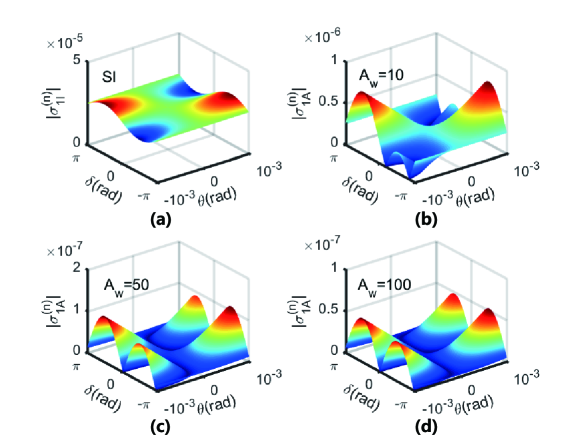
Figure 4: (Color online). The calculated results of $|\sigma_{1}^{(n)}|$ in Eq. (10) and Eq. (11) with $\eta=0.01$ and a offset $\phi=\pi$.

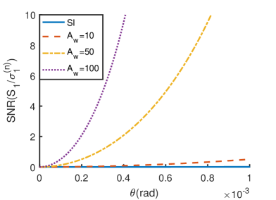
Figure 5: (Color online). The SNRs of the SI(solid line), $A_{w}=10$(dashed line), $A_{w}=50$(dash-dotted line), $A_{w}=100$(dotted line). They are calculated with $\eta=0.01$, $\delta=0$ and a offset $\phi=\pi$.

When $\phi=\pi/2$, the intensity difference in the WVAI scheme is given by

$$\Delta I_{D_{A}}(\theta)\approx(S_{2A}+\sigma_{2A}^{(n)})I_{in},$$

where

$$\left\{\begin{aligned} &S_{2A}=\frac{\theta}{4A_{w}}\\ &\sigma_{2A}^{(n)}=\eta(\frac{1-\eta}{2A_{w}^{2}}-\frac{\theta^{2}}{8}\cos\delta-\frac{\theta\sin\delta}{4A_{w}})\\ \end{aligned}\right..$$ (12)

While in the SI scheme, the intensity difference is given by

$$\Delta I_{D_{I}}(\theta)\approx I_{in}(S_{2I}+\sigma_{2I}^{(n)})I_{in},$$

where

$$\left\{\begin{aligned} &S_{2I}=\frac{\theta}{4}\\ &\sigma_{2I}^{(n)}=\eta(\frac{1-\eta}{2}-\frac{\theta^{2}}{8}\cos\delta-\frac{\theta\sin\delta}{4})\\ \end{aligned}\right..$$ (13)

Similarly, the results of $|\sigma^{(n)}|$ with $\eta=0.01$ are depicted in Fig.6. The noise in the WVAI scheme is at least 2 orders of magnitude less than the SI’s. From Fig.7, although the collected intensity in the WVAI is $1/A_{w}$ of the SI’s with the same $\theta$, the SNR of the WVAI is still higher than the SI’s.

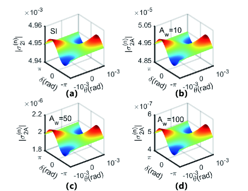
Figure 6: (Color online). The calculated results of $|\sigma_{2}^{(n)}|$ in Eq. (12) and Eq. (13) with $\eta=0.01$ and a offset $\phi=\pi/2$.

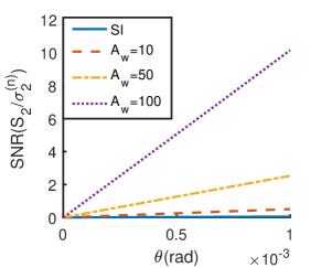
Figure 7: (Color online). The SNRs of the SI(solid line), $A_{w}=10$(dashed line), $A_{w}=50$(dash-dotted line), $A_{w}=100$(dotted line). They are calculated with $\eta=0.01$, $\delta=0$ and a offset $\phi=\pi/2$.

III.2 Fluctuations of offset $\phi$

Vibrations, air movements, deformations of optical mounts, and other environment factors may change the path difference between two arms of the interferometer. These effects cause fluctuations of $\phi$, which brings unexpected noises. Usually we use a close-loop compensation to avoid the fluctuations. However, the fluctuations can’t be eliminated at all. Consider that there’s a small fluctuation $\Delta\phi\ll 1$. $\Delta\phi$ must be less than $\theta$, otherwise the signal will be submerged in the noise. The output intensity difference is

$$\Delta I_{D_{A}}(\theta)=I_{in}(S_{3A}+\sigma_{3A}^{(n)}),$$

where

$$\left\{\begin{aligned} &S_{3A}=-\frac{I_{in}}{2Aw^{2}}\text{sin}(\phi-\frac{A_{w}\theta}{2})\text{sin}(\frac{A_{w}\theta}{2})\\ &\sigma_{3A}^{(n)}=\frac{1}{2A_{w}^{2}}\sin(\phi-A_{w}\theta+\frac{\Delta\phi}{2})\sin\frac{\Delta\phi}{2}\end{aligned}\right..$$ (14)

For the SI, one obtains

$$\Delta I_{D_{I}}(\theta)=I_{in}(S_{3I}+\sigma_{3I}^{(n)})$$

where

$$\left\{\begin{aligned} &S_{3I}=-\frac{I_{in}}{2}\text{sin}(\phi-\frac{\theta}{2})\text{sin}(\frac{\theta}{2})\\ &\sigma^{(n)}_{3I}=\frac{1}{2}\sin(\phi-\theta+\frac{\Delta\phi}{2})\sin\frac{\Delta\phi}{2}\end{aligned}\right..$$ (15)

Obviously, when $A_{w}=1$, Eq. (14) is equal to Eq. (15). Let $\phi=\pi$, $|\sigma_{3}^{(n)}|$ becomes

$$|\sigma_{3}^{(n)}| =|\frac{1}{2A_{w}^{2}}\sin(A_{w}\theta-\frac{\Delta\phi}{2})\sin\frac{\Delta\phi}{2}|$$ (16)

$$\approx|\frac{(2A_{w}\theta-\Delta\phi)\Delta\phi}{8A_{w}^{2}}|.$$

When $|\theta|\leq|\Delta\phi|$, $|\sigma_{3}^{(n)}|$ decreases monotonically along $A_{w}\geq 1$, so the noise of WVAI scheme is less than the SI’s. The SNR of the WVAI scheme could benefit from the attenuated noise. The simulated results with $\Delta\phi=10^{-4}rad$ is illustrated in Fig.8.

Figure 8: (Color online). The noise caused by the fluctuation of $\Delta\phi=10^{-4}$ at the offset $\pi$ calculated by Eq. (16).

Let $\phi=\pi/2$, Eq. (16) becomes

$$|\sigma_{3}^{(n)}| =|\frac{1}{2A_{w}^{2}}\cos(A_{w}\theta-\frac{\Delta\phi}{2})\sin\frac{\Delta\phi}{2}|$$ (17)

$$\approx|\frac{(1-A_{w}^{2}\theta^{2}-\frac{\Delta^{2}\phi}{4}+A_{w}\theta)\Delta\phi}{8A_{w}^{2}}|.$$

$|\sigma_{3}^{(n)}|$ also monotonically decreases along $A_{w}\geq 1$ when $\phi=\pi/2$. Fig.9 is the calculated diagram with $\Delta\phi=10^{-4}rad$. Apparently, the SNR of the WVAI outperforms than the SI’s with a $\pi/2$ offset.

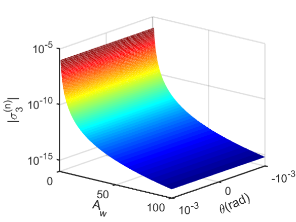
Figure 9: (Color online). The noise caused by the fluctuation of $\Delta\phi=10^{-4}$ at the offset $\pi/2$ calculated by Eq. (17).

IV Experiment

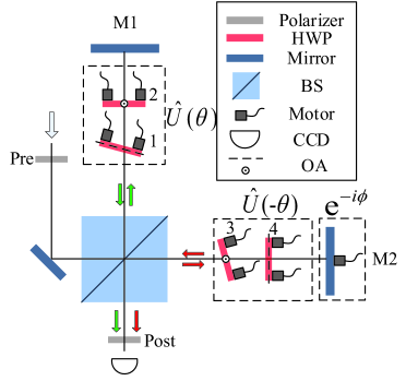
Figure 10: (Color online). The experimental setup. HWP: half wave plate. BS: 50/50beam splitter. OA: optical axis.

As mentioned in Sec. II, the results of other types of interferometer is similar to the Mach-Zehnder type’s. Because it’s easier to build and adjust, we choose a Michelson interferometer to demonstrate the proposed scheme instead. The experiment is set as illustrated in Fig.10. A monochromatic laser beam, generated by a diode laser(Toptica, DL100) with a central wavelength of $\lambda_{0}=780\text{nm}$, is prepared in the state$|\psi_{i}\rangle=1/\sqrt{2}(|H\rangle+|V\rangle)$ by the first polarizer with label ”Pre”. Then the beam enters a Michelson interferometer. The phase difference between two arms is $\phi+2n\pi$, where $n$ is integer. The difference is set by the motor fixed on the mirror M2. After the beams recombining through BS, a polarizer with label ”Post” selected them at state $|\psi_{f}\rangle=\cos\alpha|H\rangle+\sin\alpha|V\rangle$. In both arms of the interferometer, we place a two-waveplates-group to introduce a phase delay between horizontal and vertical polarization. It has been proved in Xu2013 ; Fang2016 the two-waveplates-group could equivalently realize a thin birefringent crystal. The HWPs’ OAs(optical axes) are perpendicular to each other to cancel their phase delay. Tilting one of the HWPs around its OA by a tiny angle $\gamma$ increases the optical path of this HWP, which introduce a unitary operation $\hat{U}(\theta)=e^{-i\theta A}$. In this experiment, the HWPs are binary com- pound zero-order half-wave plates, so the relationship between $\gamma$ and $\theta$ isFang2016

$$\theta=\frac{\pi(n_{e}-n_{o})h\gamma^{2}}{\lambda n^{2}},$$ (18)

where $n_{e}$, $n_{o}$, and $n$ are refractive indices of quartz for extraordinary light, ordinary light, and average light, respectively, $h$ is the thickness of the plate, and $\lambda$ is the wavelength of the light. The tilt also increase the optical path in one arms which cause a variation of offset $\phi$, so we put the HWPs into both arms to diminish this influence. As shown in Fig.10, HWP1’s and HWP4’s OAs are horizontal direction. HWP2’s and HWP3’s OAs are vertical direction. We tilt the HWP1 and HWP3 along their OAs by the same angle $\gamma$ to introduce opposite phase delay and to compensate the increased optical path length.

By rotating the postselection polarizer to a different position, we could set required $A_{w}$. The offset is set at $\pi$ for the total destructive interference. However, the minimum step size of the motor on the mirror M2 limits the practical accuracy of setting $\phi$. The vibration of the optical platform and the deformation of the motor cause fluctuations of the offset. To prove the amplification effect, we use intensity contrast ratio $I(\theta)/I(0)$ as a criterion. When $\phi>A_{w}\theta$, we obtain that

$$\frac{I(\theta)}{I(0)}=\frac{1+\cos(\phi-2A_{w}\theta)}{1+\cos\phi}.$$ (19)

When $|\psi_{f}\rangle=|H\rangle$, the experiment becomes a traditional Michelson interferometer with the path difference of $\phi-2\theta$ between two arms. In this situation the intensity contrast ratio becomes

$$\frac{I(\theta)}{I(0)}=\frac{1+\cos(\phi-2\theta)}{1+\cos\phi}.$$ (20)

which are same as the standard interferometry’s results discussed before.

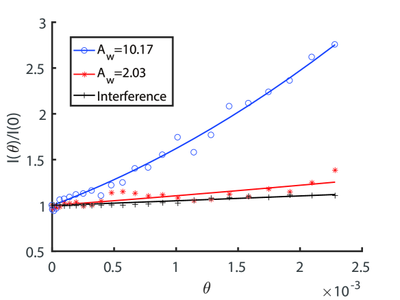
Figure 11: (Color online). Relation of the phase delay $\theta$ and intensity contrast ratio $I(\theta)/I(0)$. Blue circles, red plus signs and black asterisks are experimental results with $A_{w}=10.17,2.03$ and interference, respectively. And the corresponding lines are fitting with Eq. (19) and Eq. (20) .

The experimental results are shown in Fig.11. All curves fit well with Eq. (19) and Eq. (20). We calculate that $\phi=3.1639$, which meet the set value $\pi$ mentioned before. Apparently, the intensity contrast ratio increases along the amplification factor $A_{w}$ as predicted in Sec.II. The results firmly support the amplification effect in the WVAI scheme.

V Conclusion

In summary, we propose a new scheme named weak value amplified interferometry. The proposed scheme combines the weak value amplification and the SI. It can amplify the phase difference between different paths at a cost of decreasing the detected probability. Benefited from the amplification, the proposed scheme is robust against the technique noises. To exemplify the scheme, the investigation is based on an optical Mach-Zehnder interferometer. Comparing to the SI, the proposed scheme shows a higher intensity contrast ratio and stronger suppressions against two practical noises, which are respectively caused by the reflections of the optical elements and the fluctuations of the offset, with the offset setting at $\pi$ and $\pi/2$. To demonstrate the proposed scheme, a proof-of-principle experiment based on a Michelson interferometer is established and analyzed. The results successfully validate the phase amplification effect.

References

- (1) Scientific, L. I. G. O., B. P. Abbott, R. Abbott, T. D. Abbott, M. R. Abernathy, F. Acernese, K. Ackley et al. ”Tests of general relativity with GW150914.” Physical review letters 116, no. 22 (2016): 221101.
- (2) Monnier, John D. ”Optical interferometry in astronomy.” Reports on Progress in Physics 66, no. 5 (2003): 789.
- (3) Biegen, James F. ”Interferometric surface profiler.” U.S. Patent 4,732,483, issued March 22, 1988.
- (4) Lenef, Alan, Troy D. Hammond, Edward T. Smith, Michael S. Chapman, Richard A. Rubenstein, and David E. Pritchard. ”Rotation sensing with an atom interferometer.” Physical review letters 78, no. 5 (1997): 760.
- (5) Allen, Robert Day, Nina Strmgren Allen, and Jeffrey L. Travis. ”Video-enhanced contrast, differential interference contrast (AVEC-DIC) microscopy: A new method capable of analyzing microtubule-related motility in the reticulopodial network of allogromia laticollaris.” Cytoskeleton 1, no. 3 (1981): 291-302.
- (6) Huang, David, Eric A. Swanson, Charles P. Lin, Joel S. Schuman, William G. Stinson, Warren Chang, Michael R. Hee et al. ”Optical coherence tomography.” Science (New York, NY) 254, no. 5035 (1991): 1178.
- (7) Giovannetti, Vittorio, Seth Lloyd, and Lorenzo Maccone. ”Advances in quantum metrology.” Nature photonics 5, no. 4 (2011): 222-229.
- (8) Y. Aharonov, D. Z. Albert, and L. Vaidman, Phys. Rev. Lett. 60, 1351 (1988).
- (9) Hosten, Onur, and Paul Kwiat. ”Observation of the spin Hall effect of light via weak measurements.” Science 319, no. 5864 (2008): 787-790.
- (10) Dixon, P. Ben, David J. Starling, Andrew N. Jordan, and John C. Howell. ”Ultrasensitive beam deflection measurement via interferometric weak value amplification.” Physical review letters 102, no. 17 (2009): 173601.
- (11) Viza, Gerardo I., Juli n Mart nez-Rinc n, Gregory A. Howland, Hadas Frostig, Itay Shomroni, Barak Dayan, and John C. Howell. ”Weak-values technique for velocity measurements.” Optics letters 38, no. 16 (2013): 2949-2952.
- (12) Xu, Xiao-Ye, Yaron Kedem, Kai Sun, Lev Vaidman, Chuan-Feng Li, and Guang-Can Guo. ”Phase estimation with weak measurement using a white light source.” Physical review letters 111, no. 3 (2013): 033604.
- (13) Fang, Chen, Jing-Zheng Huang, Yang Yu, Qinzheng Li, and Guihua Zeng. ”Ultra-small time-delay estimation via a weak measurement technique with post-selection.” Journal of Physics B: Atomic, Molecular and Optical Physics 49, no. 17 (2016): 175501.
- (14) Magaa-Loaiza, Omar S., Mohammad Mirhosseini, Brandon Rodenburg, and Robert W. Boyd. ”Amplification of angular rotations using weak measurements.” Physical Review Letters 112, no. 20 (2014): 200401.
- (15) Hu, Meng-Jun, and Yong-Sheng Zhang. ”Gravitational Wave Detection via Weak Measurements.” arXiv preprint arXiv:1707.00886 (2017)
- (16) Jordan, Andrew N., Juli n Mart nez-Rinc n, and John C. Howell. ”Technical advantages for weak-value amplification: when less is more.” Physical Review X 4, no. 1 (2014): 011031.
- (17) N. Brunner and C. Simon, Phys. Rev. Lett. 105, 010405 (2010).
- (18) Li, Chuan-Feng, Xiao-Ye Xu, Jian-Shun Tang, Jin-Shi Xu, and Guang-Can Guo. ”Ultrasensitive phase estimation with white light.” Physical Review A 83, no. 4 (2011): 044102.
- (19) Denk, W., W. W. Webb, and A. J. Hudspeth. ”Mechanical properties of sensory hair bundles are reflected in their Brownian motion measured with a laser differential interferometer.” Proceedings of the National Academy of Sciences 86, no. 14 (1989): 5371-5375.
- (20) Kim, Byoung Yoon, and Herbert J. Shaw. ”Phase-reading, all-fiber-optic gyroscope.” Optics letters 9, no. 8 (1984): 378-380.
- (21) Qiu, Xiaodong, Linguo Xie, Xiong Liu, Lan Luo, Zhaoxue Li, Zhiyou Zhang, and Jinglei Du. ”Precision phase estimation based on weak-value amplification.” Applied Physics Letters 110, no. 7 (2017): 071105.
- (22) Wang, Yi-Tao, Jian-Shun Tang, Gang Hu, Jian Wang, Shang Yu, Zong-Quan Zhou, Ze-Di Cheng et al. ”Experimental demonstration of higher precision weak-value-based metrology using power recycling.” Physical review letters 117, no. 23 (2016): 230801.