Generalization Challenges for Neural Architectures in Audio Source Separation

Abstract

Recent work has shown that recurrent neural networks can be trained to separate individual speakers in a sound mixture with high fidelity. Here we explore convolutional neural network models as an alternative and show that they achieve state-of-the-art results with an order of magnitude fewer parameters. We also characterize and compare the robustness and ability of these different approaches to generalize under three different test conditions: longer time sequences, the addition of intermittent noise, and different datasets not seen during training. For the last condition, we create a new dataset, RealTalkLibri, to test source separation in real-world environments. We show that the acoustics of the environment have significant impact on the structure of the waveform and the overall performance of neural network models, with the convolutional model showing superior ability to generalize to new environments. The code for our study is available at https://github.com/ShariqM/source_separation.

1 Introduction

The sound waveform that arrives at our ears rarely comes from a single isolated source, but rather contains a complex mixture of multiple sound sources transformed in different ways by the acoustics of the environment. One of the central challenges of auditory scene analysis is to separate the components of this mixture so that individual sources may be recognized. Doing so generally requires some form of prior knowledge about the statistical structure of sound sources, such as common onset, co-modulation and continuity among harmonic components (Bregman, 1994; Darwin, 1997). Our goal is to develop a model that can learn to exploit these forms of structure in the signal in order to robustly segment the time-frequency representation of a sound waveform into its constituent sources (see Figure 1).

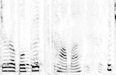
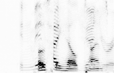
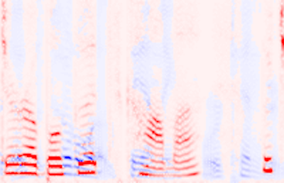
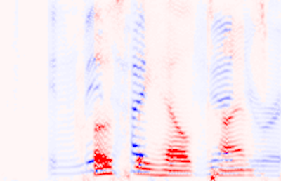
Figure 1: Left and right column: Two examples of source separation using the spectrogram of two overlapped voices as input. First row: Spectrogram of the mixture. Second Row: The source estimates using the oracle (red and blue). Third Row: Source estimates using our method.

The problem of source separation has traditionally been approached within the framework of computational auditory scene analysis (CASA) (Hu & Wang, 2013). These methods typically rely upon features such as gammatone filters in order to find a representation of the data that will allow for clustering methods to segment the individual speakers of the mixture. In some cases, these features are parameterized to allow for learning (Bach & Jordan, 2006). Other approaches use generative models such as factorial Hidden Markov Models (HMMs) to accomplish speech separation or recognition (Cooke et al., 2010). Sparse non-negative matrix factorization (SNMF) (Le Roux et al., 2015) and Bayesian non-parametric models such as (Nakano et al., 2011) have also been used. However the computational complexity inherent in many of these approaches makes them difficult to implement in an online setting that is both robust and efficient.

Recently, Hershey et al. (2016) introduced Deep Clustering (DPCL) which uses a Bi-directional Long short-term memory (BLSTM) (Graves et al., 2005) neural network to learn useful embeddings of time-frequency bins of a mixture. They formulate an objective function which encourages these embeddings to cluster according to their source so that K-means can be applied to partition the source signals in the mixture. This model was further improved in the work of Isik et al. (2016) and Chen et al. (2017) which proposed simpler end-to-end models and achieved an impressive $\sim$10.5dB Signal-to-Distortion Ratio (SDR) in the source estimation signals.

In this work we develop an alternative model for source separation based on a dilated convolutional neural network architecture (Yu & Koltun, 2015). We show that it achieves similar state-of-the-art performance as the BLSTM model with an order of magnitude fewer parameters. In addition, our convolutional approach can operate over a streaming signal enabling the possibility of source separation in real-time.

Another goal of this study is to examine how well these different neural network models generalize to inputs that are more realistic. We test the models with inputs containing very long time sequences, intermittent noise, and mixtures collected under different recording conditions, including our RealTalkLibri dataset. Success in these more challenging domains is critical for progress to continue in source separation, where the eventual goal is to be able to separate sources regardless of speaker identities, recording devices, and acoustical environments. Figure 2 shows three examples of how these factors can affect the spectrogram of the recorded waveform.

While the Automatic Speech Recognition (ASR) community has begun to discuss and address this generalization challenge (Vincent et al., 2017; Hsu et al., 2017), there has been less discussion in the context of audio source separation. In vision and machine learning, this issue is usually referred to as dataset bias (Torralba & Efros, 2011; Tzeng et al., 2017; Donahue et al., 2014) where models perform well on their training dataset but fail to generalize to new datasets. In recent years the main approach to tackling this issue has been through data augmentation. In the speech community, simulators for different acoustical environments (Barker et al., 2015; Kinoshita et al., 2013) have been leveraged to create more data.

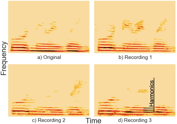
Figure 2: a: Original recording of a single female speaker from the LibriSpeech dataset; b,c,d: Recordings of the original waveform made with three different orientations between computer speaker and recording device.

Here we show that the choice of model architecture alone can improve generalization. Our choice to use a convolutional architecture was inspired by the generalization power of Convolutional Neural Networks (CNNs) (LeCun et al., 1998; Krizhevsky et al., 2012; Sigtia et al., 2016) relative to fully connected networks. We compare the performance of our CNN model with the recurrent BLSTM models of previous work and show that while both suffer when tested on reaslistic mixtures under novel recording conditions, the CNN model degrades more gracefully and exhibits superior performance to the BLSTM in this regime.

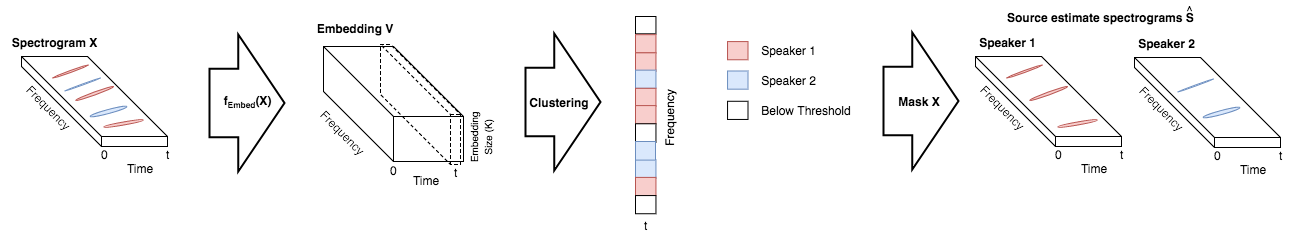
Figure 3: Overview of the source separation process.

2 Deep Attractor Framework

Notation: For a tensor $T\in\mathbf{R}^{A\times B\times C}$: $T_{\cdot,\cdot,c}\in\mathbf{R}^{A\times B}$ is a matrix, and $T_{a,\cdot,c}\in\mathbf{R}^{B}$ is a vector, and $T_{a,b,c}\in\mathbf{R}$ is a scalar.

2.1 Embedding the mixed waveform

Chen et al. (2017) propose a framework for single-channel speech separation. $x\in\mathbf{R}^{\tau}$ is a raw input signal of length $\tau$ and $X\in\mathbf{R}^{F\times T}$ is its spectrogram computed using the Short-time Fourier transform (STFT). Each time-frequency bin in the spectrogram is embedded into a K-dimensional latent space $V\in\mathbf{R}^{F\times T\times K}$ by a learnable transformation $f(\cdot;\theta)$ with parameters $\theta$:

$$\bar{V}=f(X;\theta)$$ (1)

$$V_{f,t,\cdot}=\frac{\bar{V}_{f,t,\cdot}}{||\bar{V}_{f,t,\cdot}||_{2}}$$ (2)

In our work, the embeddings are normalized to the unit sphere in the latent dimension $k$ (eq. 2).

2.2 Generating embedding labels

We assume that each time-frequency bin can be assigned to one of the $C$ possible speakers. The Ideal Binary Mask (IBM), $\bar{Y}\in\mathbf{\{0,1\}}^{F\times T\times C}$, is a one-hot representation of this classification for each time-frequency bin:

$$\bar{Y}_{f,t,c} = \begin{cases}1,&\text{if}\hskip 5.69054ptc=\underset{c^{\prime}}{\operatorname*{arg\,max}}(S_{f,t,c^{\prime}})\\ 0,&\text{otherwise}\end{cases}$$ (3)

where $S\in\mathbf{R}^{F\times T\times C}$ is the supervised source target spectrogram. We estimate $\bar{Y}$ by a mask $M\in(0,1)^{F\times T\times C}$ computed from the spectrogram $X$.

To prevent time-frequency embeddings with negligible power from interfering, the raw classification tensor $\bar{Y}$ is first masked with a threshold tensor $H\in\mathbf{R}^{F\times T}$. The threshold tensor removes time-frequency bins which are below a fraction $0<\alpha<1$ of the highest power bin present in $X$:

$$H_{f,t} = \begin{cases}0,&\text{if}\hskip 5.69054ptX_{f,t}<\alpha\hskip 2.84526pt\text{max}(X)\\ 1,&\text{otherwise}\end{cases}$$ (4)

$$Y_{\cdot,\cdot,c} = \bar{Y}_{\cdot,\cdot,c}\odot H$$ (5)

where $\odot$ denotes element-wise product.

2.3 Clustering the embedding

An attractor point, $A_{c}\in\mathbf{R}^{K}$, can be thought of as a cluster center for a corresponding source $c$. Each attractor $A_{c}$ is the mean of all the embeddings which belong to speaker $c$:

$$A_{c,k} = \frac{\sum_{f,t}V_{f,t,k}Y_{f,t,c}}{\sum_{f,t}Y_{f,t,c}}$$ (6)

During training the attractor points are calculated using the thresholded oracle mask, $Y$. In the absence of the oracle mask at test time, the attractor points are calculated using K-means. Only the embeddings which pass the corresponding time-frequency bin threshold are clustered.

Finally the mask is computed by taking the inner product of all embeddings with all attractors and applying a softmax:

$$M_{f,t,c}=\underset{c}{softmax}\Big{(}\sum_{k}A_{c,k}V_{f,t,k}\Big{)}$$ (7)

From this mask, we can compute source estimate spectrograms:

$$\hat{S}_{\cdot,\cdot,c}=M_{\cdot,\cdot,c}\odot X$$ (8)

which in turn can be converted back to an audio waveform via the inverse STFT. We do not attempt to compute the phase of the source estimates. Instead, we use the phase of the mixture to compute the inverse STFT with the magnitude source estimate spectrogram $\hat{S}$.

The loss function $\mathcal{L}$ is the mean-squared-error (MSE) of the source estimate spectrogram and the supervised source target spectrogram, $S\in\mathbf{R}^{F\times T\times C}$:

$$\mathcal{L} = \sum_{c}||S_{\cdot,\cdot,c}-\hat{S}_{\cdot,\cdot,c}||^{2}_{F}$$ (9)

where $||\cdot||_{F}$ denotes the Frobenius norm. See Figure 3 for an overview of our source separation process.

2.4 Network Architecture

A variety of neural network architectures are potential candidates to parameterize the embedding function in Equation 2. Chen et al. (2017) use a 4-layer Bi-Directional LSTM architecture (Hochreiter & Schmidhuber, 1997; Schuster & Paliwal, 1997). This architecture utilizes weight sharing across time which allows it to process inputs of variable length.

By contrast, convolutional neural networks are capable of sharing weights along both the time and frequency axis. Recently convolutional neural networks have been shown to perform state-of-the-art music transcription by having filters which convolve over both the frequency and time dimensions (Sigtia et al., 2016). One reason this may be advantageous is that the harmonic series exhibits a stationarity property in the frequency dimension. Specifically, for a signal with fundamental frequency $f_{0}$ the harmonics are equally spaced according to the following set: $\{i*f_{0}:i=2,3,...,n\}$. This structure can be seen in the equal spacing of successive harmonics in Figure 2d.

Another motivation we have for using convolutional neural networks is that they do not incorporate feedback which may allow them to be more stable under novel conditions not seen during training. In the absence of a recurrent memory, filter dilation (Yu & Koltun, 2015) enables the receptive field to integrate information over long time sequences without the loss of resolution. Furthermore, incorporating a fixed amount of future knowledge in the network is straightforward by having a fixed-lag delay in the convolution as we show in Figure 4. This is similar to fixed-lag smoothing in Kalman filters (Moore, 1973).

3 Our Model

Layer

1

2

3

4

5

6

7

8

9

10

11

12

13

Convolution

3x3

3x3

3x3

3x3

3x3

3x3

3x3

3x3

3x3

3x3

3x3

3x3

3x3

Dilation

1x1

2x2

4x4

8x8

16x16

32x32

1x1

2x2

4x4

8x8

16x16

32x32

1x1

Residual

False

True

False

True

False

True

False

True

False

True

False

True

False

Channels

128

128

128

128

128

128

128

128

128

128

128

128

K

Table 1: Dilated Convolution Model Architecture

3.1 Dilated Convolution

Yu & Koltun (2015) proposed a dilation function $D(\cdot,\cdot,\cdot;\cdot)$ to replace the pooling operations in vision tasks. For notational simplicity, we describe dilation in one dimension. This method convolves an input signal $X\in\mathbf{R}^{G}$ with a filter $K\in\mathbf{R}^{H}$ with a dilation factor $d$:

$$F_{t}=D(K,X,t;d)=\underset{dh+g=t}{\sum}K_{h}X_{g}$$

The input receptive field of a unit $F_{t}$ in an upper layer of a dilated convolutional network grows exponentially as a function of the layer number as shown in Figure 4. When applied to time sequences, this has the useful property of encoding long range time dependencies in a hierarchical manner without the loss of resolution which occurs when using pooling. Unlike recurrent networks which must store time dependencies of all scales in a single memory vector, dilated convolutions stores these dependencies in a distributed manner according to the unit and layer in the hierarchy. Lower layers encode local dependencies while higher layers encode longer range global dependencies. Such models have been successfully used for generating audio directly from the raw waveform (Oord et al., 2016).

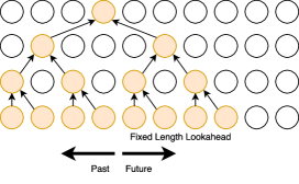
Figure 4: One-dimensional, fixed-lag dilated convolutions used by our model with dilation factors of 1, 2 and 4. The bottom row represents the input and each successive row is another layer of convolution. This network has a fixed-lag of 4 timepoints before it can output a decision for the current input.

4 Datasets

We construct our mixture data sets according to the procedure introduced in (Hershey et al., 2016), which is generated by summing two randomly selected waveforms from different speakers at signal-to-noise ratios (SNR) uniformly distributed from -5dB to 5dB and downsampled to 8kHz to reduce computational cost.

A training set is constructed using speakers from the Wall Street Journal (WSJ0) training dataset (Garofalo et al., 2007) si_tr_s.

We construct three test sets:

1) In WSJ0, a test set is constructed identical to the test set introduced in (Hershey et al., 2016) using 18 unheard speakers from si_dt_05 and si_et_05.

2) In LibriSpeech, a test set is constructed using 40 unheard speakers from test-clean.

3) In RealTalkLibri, we generate more realistic mixture using the procedure described below.

4.1 RealTalkLibri Dataset

The main motivation for creating this dataset is to record mixtures of speech where the acoustics of the room deform a high quality recording into a more realistic one. While datasets of real mixtures exist, there exists no dataset where the ground truth source waveforms are available, only the transcription of the speakers words are given as target outputs (Kinoshita et al., 2013; Barker et al., 2015). In order to understand how well our model generalizes to real world mixtures we created a small test dataset for which there is ground truth of the source waveforms.

The RealTalkLibri (RTL) test dataset is created starting from the test-clean directory of the open LibriSpeech dataset (Panayotov et al., 2015) which contains 40 speakers. We first downsampled all waveforms to 8kHz as before. Each mixture in the dataset is created by sampling two random speakers from the test-clean partition of LibriSpeech, picking a random waveform and start time for each, and playing the waveforms through two Logitech computer speakers for 12 seconds. The waveforms of the two speakers are played in separate channels linked to a left and right computer speaker, separated from the microphone of the computer by different distances. The recordings are made with a sample rate of 8kHz using a 2013 MacBook Pro (Figure 5). In order to obtain ground truth of the individual speaker waveforms each of the waveforms is played twice, once in isolation and once simultaneously with the other speaker. The first recording represents the ground truth and the second one is for the mixture. To verify the quality of the ground truth recordings, we constructed an ideal binary mask $\bar{Y}$ which performs about as well on the previous simulated datasets, see the Oracle performance in Figure 9. The RealTalkLibri data set is made up of two recording sessions which each yielded 4.5 hours of data, giving us a total of 9 hours of test data. The data is available at https://www.dropbox.com/s/4pscejhkqdr8xrk/rtl.tar.gz?dl=0

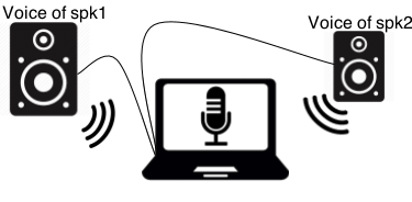
Figure 5: Recording setup diagram.

5 Experiments

5.1 Experimental Setup

We evaluate the models on a single-channel simultaneous speech separation task. The mixture waveforms are transformed into a time-frequency representation using the Short-time Fourier Transform (STFT) and the log-magnitude features, $X$, are served as input to the model. The STFT is computed with 32ms window length, 8ms hop size, and the Hann window. We use SciPy (Jones et al., 2014) to compute the STFT and TensorFlow to build our neural networks (Abadi et al., 2016).

We report our results using a distance measure between the source estimate and the true source in the waveform space. Our distance measure is the signal-to-distortion ratio (SDR) which was introduced in (Vincent et al., 2006) as a blind audio source separation (BSS) metric which is less sensitive to the gain of the source estimate. We compute our results using version 3 of the Matlab bsseval toolbox (Févotte et al., 2005). A python implementation of this code is also available online (Raffel et al., 2014) .

Our network consists of 13 dilated convolutional layers (Yu & Koltun, 2015) made up of two stacks, each stack having its dilation factor double each layer. Batch Normalization (Ioffe & Szegedy, 2015) is applied to each layer and residual connections (He et al., 2016) are used at every other layer, see Table 1 for details. Our model has a fixed-lag response of 127 timepoints ($\sim$ 1s, see Figure 4). The output of the network is of dimensionality ($T\times F\times K$), $T$ being the number of output time points, F the number of frequency bins, and $K$ being both the final number of channels and embedding dimensionality. During training $T$ is set to 400 ($\sim$3s), $F$ to 129 (specified by the STFT), $K$ to 20, and $\alpha$ (threshold factor) to 0.6. For evaluation we also use the max() function rather than the softmax() for computing the mask in equation (7). The Adam Optimizer (Kingma & Ba, 2014) is used with a piecewise learning rate schedule, boundaries$=[10k,50k,100k]$, values $=[1.0,0.5,0.1,0.01]$, and initial learning rate $1\mathrm{e}{-3}$.

We reimplement the DANet of (Chen et al., 2017) with a BLSTM architecture containing 4 layers and 500 hidden units in both the forward and backward LSTM, for a total of 1000 hidden units. We replicated their training schedule using the RMSProp algorithm (Tieleman & Hinton, 2012), a starting learning rate of $1\mathrm{e}{-3}$, and exponential decay with parameters: decay_steps$=2000$, decay_rate$=0.95$.

We calculate an Oracle score using the Ideal Binary Mask (IBM), $\bar{Y}$, using the ground truth source spectrograms (Eq. 3).

5.2 WSJ0 Evaluation

We begin by evaluating the models on the WSJ0 test dataset as in (Chen et al., 2017). Our state-of-the-art results are shown in Table 2. Our model achieves the best score using a factor of ten fewer parameters than DANet. The DPCL score is taken from (Isik et al., 2016) which has a very similar architecture to DANet and therefore a similar number of parameters. Their model has one important difference however, a second neural network is used to enhance the source estimate spectrogram to achieve their result. Our model is still able to exceed its performance without this extra enhancement network. In addition, our model has a fixed window into the future whereas the BLSTM models have access to the entire future. This indicates that a convolution based architecture is better at solving this source separation task with less information in comparison to a recurrent based architecture.

Model	WSJ0	Number of
	SDR (dB)	Parameters
DANet (BLSTM)	10.48	$17\,114\,580$
DPCL* (BLSTM)	10.8	?
Ours (CNN)	10.97	$1\,650\,836$
Oracle	13.49	-

Table 2: Signal-to-Distortion Ratio (SDR) for two competitor models, our proposed convolutional model, and the Oracle. Our model achieves the best results using significantly fewer parameters. Our score is averaged over 3200 examples. *: SDR score is from (Isik et al., 2016). This model is at an advantage because it has a second enhancement neural network that improved the source estimate spectrogram after masking in addition to the normal BLSTM.

5.3 Embeddings

At test time we do not have access to the labels $\bar{Y}$ so the attractors cannot be computed using equation 6. As in previous work, K-means is employed instead. In order for the attractors to from a good proxy for the K-means algorithm it is important the attractors form dense clusters of embeddings. Without applying any regularization on the attractors we found that this was not the case. The main issue we observed was that embeddings for both speakers in the mixture were largely overlapping with a few embeddings driven extremely far apart in order to drive the attractors apart. This worked well for training but poorly at test time, the solutions found by K-means didn’t match the attractors found in training. In order to combat this degeneracy we l2 normalize the embeddings V which is novel and very effective (Eq. 2).

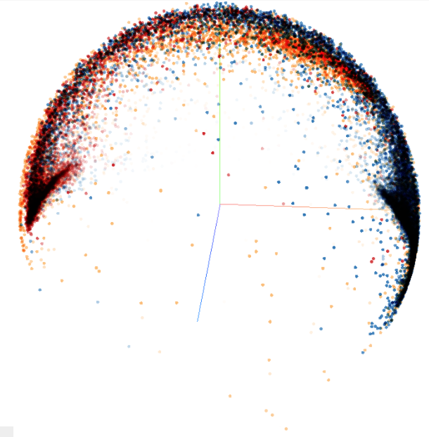
Figure 6: Embeddings for two speakers (red & blue) over 200 time points, projected onto a 3-dimensional subspace using PCA. The orange points correspond to time-frequency bins where the energy was below threshold (see eq. 5). There are $T\times F=200\times 129=25800$ embedding points in total.

In Figure 6 we visualize the embedding outputs of our model using PCA for a single mixture across $T=200$ timepoints. Each embedding point corresponds to a single time-frequency bin in the mixed input spectrogram. The embeddings are colored in this diagram according to the oracle labelling, red for speaker 1 and blue for speaker 2. Notice that the network has learned to cluster the embeddings according to the speaker they belong too, i.e. there is a high density of red embeddings on the left and similarly for blue embeddings on the right. This structure allows K-means to easily find cluster centers that match the attractors used at training time.

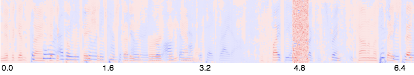
Figure 7: Source separation spectrogram for the noise generalization experiment.

5.4 Generalization Experiments

5.4.1 Length Generalization

In the first experiment we study how well these models work under time-sequences 25x longer than they are trained on, i.e. $T=10000$ ($\sim 80$s). Previous work (Kaiser & Sutskever, 2015) has indicated that because recurrent architectures incorporate feedback they can function unpredictably for sequence lengths beyond those seen during training. On the other hand, convolutional network architectures do not incorporate any feedback. This is advantageous for processing time sequences of indefinite length because errors cannot accumulate over time. Since a convolutional network is a stationary process in the convolved dimension, we hypothesize this architecture will operate more robustly over sequence lengths much longer than those seen during training. Our results are shown in Figure 8a. Surprisingly, the results indicate that the BLSTM is also able to generalize to sequences of significantly larger length, contrary to our expectations. We discuss possible explanations of this result in the next section. Our CNN model is able to maintain its performance across the long sequence as expected.

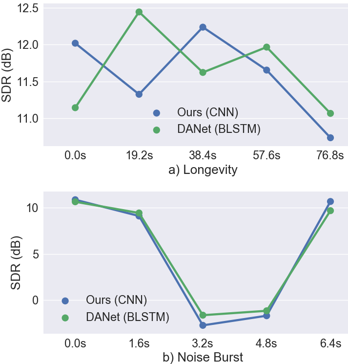
Figure 8: Results of the length and noise generalization experiments. For both plots, we plot the SDR starting at the time specified by the x-axis up until 400 time points ($\sim 3$s) later. Both the BLSTM and CNN are (a) able to operate over very long time sequences and (b) recover from intermittent noise. See Figure 7 for the spectrogram in b).

5.4.2 Noise Generalization

In the second experiment we are interested in how the models respond to small bursts of input data far outside of the training distribution. We believe the BLSTM model might become unstable as a result of such inputs because its recurrent structure makes it possible for the noise to affect its hidden state indefinitely. We took sequences of length $T=1200$ ($\sim 9$s) and inserted white noise for 0.25s in the middle of the mixture to disrupt the models process. Our results are shown in Figure 8b. Again, contrary to our belief the BLSTM is very resilient to this noise, the model quickly recovers after the noise passes (last data point). One possible explanation is that the BLSTM is only integrating information over short time scales and therefore “forgets” about previous input data after a short number of time steps. We believe this is because when we construct the input for our models we randomly sample a starting time for each waveform. This may force the BLSTM to learn a stationary function since it must be able to separate the mixture with or without information from the past in its hidden state.

5.4.3 Data Generalization

In the final experiment we are interested in how well the models generalize to data progressively farther from their training distribution. We trained all the models on the WSJ0 training set and then tested on the WSJ0 test set, the LibriSpeech test set, and RealTalkLibri test set. Our results are shown in Figure 9. Our model generalizes quite well from the WSJ0 dataset to the LibriSpeech dataset, only losing $1.8$dB of performance. Unfortunately it degrades substantially, by $7.5$dB, when using the RTL dataset. However, our model still outperforms the DANet model on all datasets. Note that the Oracle performance also degrades by $\sim 1$dB on RTL.

In Figure 10 we visualize the mistakes our network makes under the RealTalkLibri dataset. The first example indicates that the model does not have a strong enough bias to the harmonic structure contained in speech, it classifies the frequencies of the fundamental to a different speaker than the harmonic frequencies of that fundamental. The second example indicates that the model also has issues with temporal continuity, the speaker identity of particular frequency bins varies sporadically across time. This indicates that there is still room to improve generalization in these models by modifying model architecture and adding regularization.

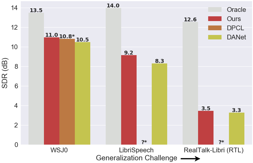
Figure 9: Results of models tested on WSJ0 simulated mixtures, LibriSpeech simulated mixtures, and our RealTalkLibri (RTL) dataset. Our model performs the best on WSJ0, generalizes better to LibriSpeech, but fails alongside the BLSTM at generalizing to the real mixtures of RTL. All models are trained on WSJ0. *: Model has a second neural network to enhance the source estimate spectrogram and is therefore at an advantage. The model wasn’t available online for testing against LibriSpeech or RTL.

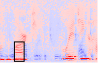
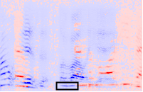
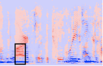
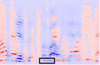
Figure 10: Left and right column: Two examples of source separation on the RealTalkLibri dataset. Row 1: Source estimates using the oracle. Row 2: The source estimates using our method. The model has difficulty maintaining continuity of speaker identity across frequencies of a harmonic stack (left column) and across time (right column).

6 Discussion

Recurrent neural networks have been shown to perform audio source separation with high fidelity. Here we explored using convolutional neural networks as an alternative model. Our state-of-the-art results on the WSJ0 dataset using a factor of ten fewer parameters show that convolutional models are both more accurate and more efficient for audio source separation. Our model has the additional advantage of working online with a fixed-lag response of $\sim 1$sec.

In order to study the robustness of all models we studied their performance under three different conditions: longer time sequences, intermittent noise, and datasets not seen during training. Our results in the length and noise generalization experiments indicate that the BLSTM learns to behave much like a stationary process in the temporal dimension. We do not observe any substantial degradation in performance after it has been perturbed with noise. It also performs consistently on sequences which are significantly longer than those seen during training.

On the other hand, we get this stationarity property for free with our convolutional model. This further motivates our network architecture in Figure 4 which, by design, integrates only local information from the past and future.

In the final experiment we showed that our convolutional neural network also generalized better to both the LibriSpeech dataset and the RealTalkLibri dataset we introduced here. Models which are robust to new datasets as well as the deformations caused by the acoustics of different environments are critical to progress in audio source separation. Our RealTalkLibri dataset complements other real-world speech datasets (Barker et al., 2015; Kinoshita et al., 2013) by additionally providing approximate ground truth waveforms for the mixture which is currently not available.

Looking forward, we aim to improve the generalization ability on examples such as those shown in Figure 10 by introducing a training set for RealTalkLibri, developing more robust model architectures, introducing regularizers for the structure of speech, and creating powerful data augmentation tools. We also believe models which can operate under an unknown number of sources is of utmost importance to the field of audio source separation.

References

- Abadi et al. (2016) Abadi, Martín, Barham, Paul, Chen, Jianmin, Chen, Zhifeng, Davis, Andy, Dean, Jeffrey, Devin, Matthieu, Ghemawat, Sanjay, Irving, Geoffrey, Isard, Michael, et al. Tensorflow: A system for large-scale machine learning. In OSDI, volume 16, pp. 265–283, 2016.
- Bach & Jordan (2006) Bach, Francis R and Jordan, Michael I. Learning spectral clustering, with application to speech separation. Journal of Machine Learning Research, 7(Oct):1963–2001, 2006.
- Barker et al. (2015) Barker, Jon, Marxer, Ricard, Vincent, Emmanuel, and Watanabe, Shinji. The third ‘chime’speech separation and recognition challenge: Dataset, task and baselines. In Automatic Speech Recognition and Understanding (ASRU), 2015 IEEE Workshop on, pp. 504–511. IEEE, 2015.
- Bregman (1994) Bregman, Albert S. Auditory scene analysis: The perceptual organization of sound. MIT press, 1994.
- Chen et al. (2017) Chen, Zhuo, Luo, Yi, and Mesgarani, Nima. Deep attractor network for single-microphone speaker separation. In Acoustics, Speech and Signal Processing (ICASSP), 2017 IEEE International Conference on, pp. 246–250. IEEE, 2017.
- Cooke et al. (2010) Cooke, Martin, Hershey, John R, and Rennie, Steven J. Monaural speech separation and recognition challenge. Computer Speech & Language, 24(1):1–15, 2010.
- Darwin (1997) Darwin, Chris J. Auditory grouping. Trends in cognitive sciences, 1(9):327–333, 1997.
- Donahue et al. (2014) Donahue, Jeff, Jia, Yangqing, Vinyals, Oriol, Hoffman, Judy, Zhang, Ning, Tzeng, Eric, and Darrell, Trevor. Decaf: A deep convolutional activation feature for generic visual recognition. In International conference on machine learning, pp. 647–655, 2014.
- Févotte et al. (2005) Févotte, Cédric, Gribonval, Rémi, and Vincent, Emmanuel. Bss_eval toolbox user guide–revision 2.0. 2005.
- Garofalo et al. (2007) Garofalo, John, Graff, David, Paul, Doug, and Pallett, David. Csr-i (wsj0) complete. Linguistic Data Consortium, Philadelphia, 2007.
- Graves et al. (2005) Graves, Alex, Fernández, Santiago, and Schmidhuber, Jürgen. Bidirectional lstm networks for improved phoneme classification and recognition. Artificial Neural Networks: Formal Models and Their Applications–ICANN 2005, pp. 753–753, 2005.
- He et al. (2016) He, Kaiming, Zhang, Xiangyu, Ren, Shaoqing, and Sun, Jian. Deep residual learning for image recognition. In Proceedings of the IEEE conference on computer vision and pattern recognition, pp. 770–778, 2016.
- Hershey et al. (2016) Hershey, John R, Chen, Zhuo, Le Roux, Jonathan, and Watanabe, Shinji. Deep clustering: Discriminative embeddings for segmentation and separation. In Acoustics, Speech and Signal Processing (ICASSP), 2016 IEEE International Conference on, pp. 31–35. IEEE, 2016.
- Hochreiter & Schmidhuber (1997) Hochreiter, Sepp and Schmidhuber, Jürgen. Long short-term memory. Neural computation, 9(8):1735–1780, 1997.
- Hsu et al. (2017) Hsu, Wei-Ning, Zhang, Yu, and Glass, James. Unsupervised domain adaptation for robust speech recognition via variational autoencoder-based data augmentation. arXiv preprint arXiv:1707.06265, 2017.
- Hu & Wang (2013) Hu, Ke and Wang, DeLiang. An unsupervised approach to cochannel speech separation. IEEE Transactions on audio, speech, and language processing, 21(1):122–131, 2013.
- Ioffe & Szegedy (2015) Ioffe, Sergey and Szegedy, Christian. Batch normalization: Accelerating deep network training by reducing internal covariate shift. In International Conference on Machine Learning, pp. 448–456, 2015.
- Isik et al. (2016) Isik, Yusuf, Roux, Jonathan Le, Chen, Zhuo, Watanabe, Shinji, and Hershey, John R. Single-channel multi-speaker separation using deep clustering. arXiv preprint arXiv:1607.02173, 2016.
- Jones et al. (2014) Jones, Eric, Oliphant, Travis, and Peterson, Pearu. SciPy: open source scientific tools for Python. 2014.
- Kaiser & Sutskever (2015) Kaiser, Łukasz and Sutskever, Ilya. Neural gpus learn algorithms. arXiv preprint arXiv:1511.08228, 2015.
- Kingma & Ba (2014) Kingma, Diederik P and Ba, Jimmy. Adam: A method for stochastic optimization. arXiv preprint arXiv:1412.6980, 2014.
- Kinoshita et al. (2013) Kinoshita, Keisuke, Delcroix, Marc, Yoshioka, Takuya, Nakatani, Tomohiro, Sehr, Armin, Kellermann, Walter, and Maas, Roland. The reverb challenge: A common evaluation framework for dereverberation and recognition of reverberant speech. In Applications of Signal Processing to Audio and Acoustics (WASPAA), 2013 IEEE Workshop on, pp. 1–4. IEEE, 2013.
- Krizhevsky et al. (2012) Krizhevsky, Alex, Sutskever, Ilya, and Hinton, Geoffrey E. Imagenet classification with deep convolutional neural networks. In Advances in neural information processing systems, pp. 1097–1105, 2012.
- Le Roux et al. (2015) Le Roux, Jonathan, Weninger, Felix J, and Hershey, John R. Sparse nmf–half-baked or well done? Mitsubishi Electric Research Labs (MERL), Cambridge, MA, USA, Tech. Rep., no. TR2015-023, 2015.
- LeCun et al. (1998) LeCun, Yann, Bottou, Léon, Bengio, Yoshua, and Haffner, Patrick. Gradient-based learning applied to document recognition. Proceedings of the IEEE, 86(11):2278–2324, 1998.
- Moore (1973) Moore, John B. Discrete-time fixed-lag smoothing algorithms. Automatica, 9(2):163–173, 1973.
- Nakano et al. (2011) Nakano, Masahiro, Le Roux, Jonathan, Kameoka, Hirokazu, Nakamura, Tomohiko, Ono, Nobutaka, and Sagayama, Shigeki. Bayesian nonparametric spectrogram modeling based on infinite factorial infinite hidden markov model. In Applications of Signal Processing to Audio and Acoustics (WASPAA), 2011 IEEE Workshop on, pp. 325–328. IEEE, 2011.
- Oord et al. (2016) Oord, Aaron van den, Dieleman, Sander, Zen, Heiga, Simonyan, Karen, Vinyals, Oriol, Graves, Alex, Kalchbrenner, Nal, Senior, Andrew, and Kavukcuoglu, Koray. Wavenet: A generative model for raw audio. arXiv preprint arXiv:1609.03499, 2016.
- Panayotov et al. (2015) Panayotov, Vassil, Chen, Guoguo, Povey, Daniel, and Khudanpur, Sanjeev. Librispeech: an asr corpus based on public domain audio books. In Acoustics, Speech and Signal Processing (ICASSP), 2015 IEEE International Conference on, pp. 5206–5210. IEEE, 2015.
- Raffel et al. (2014) Raffel, Colin, McFee, Brian, Humphrey, Eric J, Salamon, Justin, Nieto, Oriol, Liang, Dawen, Ellis, Daniel PW, and Raffel, C Colin. mir_eval: A transparent implementation of common mir metrics. In In Proceedings of the 15th International Society for Music Information Retrieval Conference, ISMIR. Citeseer, 2014.
- Schuster & Paliwal (1997) Schuster, Mike and Paliwal, Kuldip K. Bidirectional recurrent neural networks. IEEE Transactions on Signal Processing, 45(11):2673–2681, 1997.
- Sigtia et al. (2016) Sigtia, Siddharth, Benetos, Emmanouil, and Dixon, Simon. An end-to-end neural network for polyphonic piano music transcription. IEEE/ACM Transactions on Audio, Speech and Language Processing (TASLP), 24(5):927–939, 2016.
- Tieleman & Hinton (2012) Tieleman, Tijmen and Hinton, Geoffrey. Lecture 6.5-rmsprop: Divide the gradient by a running average of its recent magnitude. COURSERA: Neural networks for machine learning, 4(2):26–31, 2012.
- Torralba & Efros (2011) Torralba, Antonio and Efros, Alexei A. Unbiased look at dataset bias. In Computer Vision and Pattern Recognition (CVPR), 2011 IEEE Conference on, pp. 1521–1528. IEEE, 2011.
- Tzeng et al. (2017) Tzeng, Eric, Hoffman, Judy, Saenko, Kate, and Darrell, Trevor. Adversarial discriminative domain adaptation. In Computer Vision and Pattern Recognition (CVPR), volume 1, pp. 4, 2017.
- Vincent et al. (2006) Vincent, Emmanuel, Gribonval, Rémi, and Févotte, Cédric. Performance measurement in blind audio source separation. IEEE transactions on audio, speech, and language processing, 14(4):1462–1469, 2006.
- Vincent et al. (2017) Vincent, Emmanuel, Watanabe, Shinji, Nugraha, Aditya Arie, Barker, Jon, and Marxer, Ricard. An analysis of environment, microphone and data simulation mismatches in robust speech recognition. Computer Speech & Language, 46:535–557, 2017.
- Yu & Koltun (2015) Yu, Fisher and Koltun, Vladlen. Multi-scale context aggregation by dilated convolutions. arXiv preprint arXiv:1511.07122, 2015.