Abstract

Using the volume of the space enclosed by the Ryu-Takayanagi (RT) surface, we study the complexity of the disk-shape subregion (with radius R) in various (2+1)-dimensional gapped systems with gravity dual. These systems include a class of toy models with singular IR and the bottom-up models for quantum chromodynamics and fractional quantum Hall effects. Two main results are: i) in the large-R expansion of the complexity, the R-linear term is always absent, similar to the absence of topological entanglement entropy; ii) when the entanglement entropy exhibits the classic ‘swallowtail’ phase transition, the complexity is sensitive but reacts differently.

1 Introduction

Holographic principle suggests that the spacetime could be an emergent phenomenon. Entanglement, which characterizes how the joint of different parts of a system distinguishes its classical whole, is believed to play an essential role [1, 2]. This insight is due in large part to the holographic prescription for the entanglement entropy—the area of the codimension-two minimal surface in the bulk with its UV boundary coincident with the entangling surface in the dual field theory [3]. The mentioned minimal surface has been referred as the Ryu-Takayanagi (RT) surface.

Complexity is another quantum information quantity that might be important in understanding the quantum structure of spacetimes [4]. It is relevant to the number of unitary operators which converts one quantum state to another. There are two holographic dualities which have been proposed to describe the complexity. Popularly, they are known as the ‘complexity=volume’ (CV) conjecture [5] and ‘complexity=action’ (CA) conjecture [6]. Starting from the study of the linear growth of the black hole formation and the size of the Einstein-Rosen bridge, the former conjecture states that the complexity in the boundary field theory is related to the volume of a codimension-one maximal bulk space, which is anchored on a given boundary time slice. The CV conjecture needs to introduce a length scale which depends on the concrete systems. Without such arbitrariness, the latter conjecture states that the complexity is described by the bulk action on the Wheeler-DeWitt patch [6], which is the domain of dependence of any Cauchy surfaces in the bulk that approaches the boundary time slice.

In this paper, we will be concerned with the RT volume that is associated with the bulk space enclosed by the RT surface. Intuitively, the RT volume is interesting since it is intrinsically related to the holographic entanglement entropy (HEE). The lesson learned from the RT volume would suggest new holographic duals to the quantum information. In fact, motivated by the connection between the volume of the maximal time slice in an Anti-de Sitter (AdS) spacetime and the fidelity susceptibility of pure states [7], the RT volume was proposed as the holographic subregion complexity (HSC), corresponding to the reduced fidelity susceptibility of mixed states in the boundary [8, 9]. Furthermore, the quantitative evidence of this correspondence has been presented by studying the marginal perturbation in the (1+1)-dimensional conformal field theory (CFT) [10]. Moreover, for a spherical subregion in the boundary, it was also argued that the regularized RT volume is related to the Fisher information metric [11]. On the other hand, the HSC has a deep relationship to the HEE indeed. For example, similar to the HEE, the HSC can signal different phase transitions [12, 13, 14]. Besides the aforementioned work, the RT volume has attracted much attention, e.g., see [15, 16, 17, 18, 19]. Among others, we only note that the scale arbitrariness in the CV conjecture could be eliminated by introducing some variant of the RT volume: it was proposed recently within the AdS₃/CFT₂ duality that the curvature integral in the space enclosed by the RT surface provides a dimensionless quantity which could be dual to the complexity of the reduced density matrix [20].

For condensed matter theories (CMT), the quantum entanglement provides important insight into the structure of many-body states. One famous example is the notion of topological entanglement entropy (TEE) [21, 22, 23], which is one of the most proximate representations of the topological order in (2+1)-dimensional topological field theories. The TEE can be extracted by the asymptotic behavior of the entanglement entropy between a disk (with radius R) and the rest of the system: $\mathcal{S}=\alpha R-\mathcal{S}_{\mathrm{top}}+\mathcal{O}(R^{-1})$. Here the first term denotes the well-known area law and the second term is the TEE. When the theory has a mass gap, the TEE is invariant under a continuous deformation of the disk.

In [24], the TEE is studied based on the RT prescription. It is found that the TEE is vanishing for the AdS soliton, as expected for a theory like quantum chromodynamics (QCD). The vanishing of the holographic TEE is not accidental, which also can be seen in a class of (2+1)-dimensional gapped geometries with singular IR [25, 26]. The nonvanishing TEE can be produced by introducing the Chern-Simons interaction in the D3-D7 systems [27] or the Gauss-Bonnet (GB) curvature in the gravity theory when the RT surface has the disk topology [28]. Moreover, the TEE can be interpreted as the black hole entropy in the AdS₃ [29, 30].

A natural question is whether there is a quantity in the HSC, which corresponds to the TEE in the HEE. As a first step to address this question, we will study the large-R expansion of the HSC (with a disk-shape subregion) in various (2+1)-dimensional holographic gapped systems without the TEE. On the other hand, in some of these systems, the HEE can exhibit a classic ‘swallowtail’ phase transition when the topology of the RT surface changes from the disk shape to the cylinder shape. This typical phenomenon has been taken as a probe of the confinement/deconfinement transition [31, 32, 24]. We will study the HSC in the intermediate-R region and focus on whether the HSC is sensitive to the topology change of the RT surface.

The rest of this paper is organized as follows. In Sec. 2, we will study a class of gapped geometries

$$ds^{2}=\frac{L^{2}}{z^{2}}\left[-h(z)dt^{2}+d\rho^{2}+\rho^{2}d\theta^{2}+\frac{dz^{2}}{f(z)}\right],$$ (1)

where $L$ is the AdS radius and the IR behavior $\left(z\rightarrow\infty\right)$ is required to be

$$f(z)=az^{n}+\cdots,\quad a>0,\;n\geq 2.$$ (2)

Then the spacetime becomes singular in the IR. We will prove analytically that in the large-R expansion, the R-linear term is absent in the HSC. Moreover, we will calculate numerically the HSC as a function of R in several toy-models. It will be shown that the HSC can probe the topology change of the RT surface. From Sec. 3 to Sec. 5, we will study three kinds of (2+1)-dimensional phenomenon models with the mass gap, including the AdS soliton, soft-wall model and holographic fractional quantum Hall (FQH) model. For all the models, the R-linear term in the HSC is vanishing. For the AdS soliton, the HSC is sensitive to the topology change. In Sec. 6, we will discuss whether the R-linear term can be produced in the soft-wall model by involving the GB correction to the gravity theory. In Sec. 7, the conclusion will be given. In Appendix A, we will review briefly the numerical solution of the holographic FQH model. In Appendix B, we attempt to explore further the HSC in the GB gravity.

2 Geometries with singular IR

Suppose that a spacetime is described by the metric (1) with the IR behavior (2). When $n>0$, the singularity lies at a finite proper distance away. From the UV/IR connection, it might be excepted that the corresponding IR phase is gapped. Actually, by analyzing the spectrum of a probed scalar field in the spacetime, it has been found [25, 26] that the system with $n>2$ has a discrete spectrum and for $n=2$, it has a continuous spectrum above the gap. For $0<n<2$, the geometry is singular but is not dual to a gapped phase.

2.1 RT surface

We will study the RT surfaces in those gapped geometries. Consider a circle with radius R in the UV boundary, which divides the system into two parts. The HEE between them can be determined by

$$\mathcal{S}=\frac{\mathrm{Area}\left(\Sigma\right)}{4G_{N}},$$ (3)

where $G_{N}$ is the four-dimensional Newton constant and $\Sigma$ denotes the minimal surface that extends from the boundary circle to the bulk. Using Eq. (1), one can read the induced metric of the RT surface:

$$ds_{\mathrm{ind}}^{2}=\frac{L^{2}}{z^{2}}\left[(\frac{1}{f}+\rho^{\prime 2})dz^{2}+\rho^{2}d\theta^{2}\right],$$ (4)

where the prime denotes the derivative with respect to $z$ that is taken as one of surface coordinates. By the induced metric, one can obtain the entropy functional of $\rho(z)$:

$$\mathcal{S}=\frac{\pi L^{2}}{2G_{N}}\int_{0}^{\infty}dz\frac{\rho}{z^{2}}\sqrt{\frac{1}{f}+\rho^{\prime 2}}.$$ (5)

Taking the variation with respect to $\rho(z)$, one can derive the equation of motion (EOM) that determines the extremal surface:

$$\rho^{\prime\prime}-\frac{2f\rho^{\prime 3}}{z}-\frac{\rho^{\prime 2}}{\rho}-\left(\frac{2}{z}-\frac{f^{\prime}}{2f}\right)\rho^{\prime}-\frac{1}{\rho f}=0\text{.}$$ (6)

If there are several extremal surfaces, the entropy functional is multi-valued and the HEE is given by the minimal value.

2.2 HEE and HSC

2.2.1 Large R expansion

In Ref. [25], it has been pointed out that for $n=2$, the RT surface only can be disk-like. While for $n>2$, the topology can be changed from disk to cylinder as R increases, see Figure 6 in [25] for a schematic. In particular, we stress that for $n>2$ only a cylinder-like RT surface can appear at large R.

Usually, it is not possible to solve the EOM for RT surfaces analytically. But when R is large, the analytical solutions have been found in [26] by a matching procedure. Let’s briefly review the strategy. In the UV, one can find that $\rho(z)$ can be expanded in 1/R as

$$\rho(z)=R-\frac{\rho_{1}(z)}{R}-\frac{\rho_{3}(z)}{R^{3}}+\cdots-\frac{\hat{\rho}(z)}{R^{v}}+\cdots,$$ (7)

where the last term denotes the leading term of those that are not odd powers of 1/R. We will focus on $n>2$ at first. For our aim, it is enough to keep only the pending function $\rho_{1}(z)$. In terms of the EOM (6), $\rho_{1}(z)$ should satisfy

$$\frac{z^{2}}{\sqrt{f}}(\frac{\sqrt{f}}{z^{2}}\rho_{1}^{\prime})^{\prime}=s_{1},$$ (8)

where the source is $s_{1}=-1/f$. Equation (8) has the solution

$$\rho_{1}(z)=\int_{0}^{z}du\frac{u^{2}}{\sqrt{f(u)}}(b_{1}+\int_{u}^{\infty}dv\frac{1}{v^{2}\sqrt{f(v)}}),$$ (9)

where $b_{1}$ is an integration constant. In the IR, the EOM (6) implies that $\rho(z)$ has the large $z$ expansion

$$\rho(z)=\rho_{0}+\frac{2z^{2-n}}{\rho_{0}a(n-2)(n+2)}+\cdots,\quad n>2.$$ (10)

This is a cylinder-like solution. The constant $\rho_{0}$ means the radius of the cylinder in the IR. To match the UV and IR, the solution (9) is pulled to a sufficiently large $z$ so that Eq. (2) holds. Then one has

$$\rho_{1}(z)=\frac{b_{1}}{\sqrt{a}}\frac{z^{3-n/2}}{3-n/2}(1+\cdots)+\frac{2z^{2-n}}{(2-n)(2+n)a}(1+\cdots).$$ (11)

After inserting Eq. (11) into the UV expansion (7), it can be matched to the IR expansion (10), which leads to

$$b_{1}=0,\quad\rho_{0}=R.$$ (12)

Now one has a large-R solution applied to the total region of $z$. Calculating Eq. (5) with this solution, one can obtain

$$\mathcal{S}\sim R\int_{0}^{\infty}dz\frac{1}{z^{2}\sqrt{f(z)}}-\frac{1}{R}\int_{0}^{\infty}dz\frac{\sqrt{f(z)}}{2z^{2}}\rho_{1}^{\prime}(z)^{2}+\mathcal{O}(\frac{1}{R^{3}}),$$ (13)

where $\rho_{1}(z)$ is given by Eq. (11) and Eq. (12). One can see that the TEE is zero.

The matching procedure for $n=2$ is similar. The final solution can be written as

$$\rho(z)=R-\frac{1}{2\sqrt{a}}(\frac{b_{1}}{R}+\cdots)z^{2}-\frac{1}{2aR}\log{z}+\cdots,$$ (14)

where $b_{1}=0$. Plugging Eq. (14) into the entropy functional (5) leads to

$$\mathcal{S}\sim R\int_{0}^{\infty}dz\frac{1}{z^{2}\sqrt{f(z)}}+\frac{1}{R}\int_{0}^{\infty}dz\frac{f(z)-4az^{2}\log{z}}{8a^{2}z^{4}\sqrt{f(z)}}+\mathcal{O}(\frac{1}{R^{3}}),$$ (15)

where the TEE is still zero.

Now we will calculate the HSC. Consider the volume of the space enclosed by the RT surface. The HSC can be defined by [8]:

$$\mathcal{C}=\frac{\mathrm{Volume}\left(\Sigma\right)}{8\pi LG_{N}},$$ (16)

where $L$ is supposed to be the AdS radius. It should be noted that the suitable length scale for a gapped phase might not be determined by the AdS radius alone. In this paper, we will not explore this issue since we focus on comparing the area of RT surfaces and the RT volume. Moreover, for the similar reason, we don’t care about other proposals for the holographic complexity.

From the metric (1) with the constant time, one can obtain the complexity functional:

$$\mathcal{C}=\frac{L^{2}}{4G_{N}}\int_{0}^{\infty}dz\frac{1}{z^{3}\sqrt{f(z)}}\int_{0}^{\rho(z)}d\rho\rho.$$ (17)

Using the large-R expansion of $\rho(z)$, we can expand Eq. (17) to

$$\mathcal{C}\sim\left\{\begin{array}[]{c}R^{2}\int_{0}^{\infty}dz\frac{1}{z^{3}\sqrt{f(z)}}-\int_{0}^{\infty}dz\frac{2\rho_{1}(z)}{z^{3}\sqrt{f(z)}}+\mathcal{O}(\frac{1}{R^{2}}),\;n>2;\\ R^{2}\int_{0}^{\infty}dz\frac{1}{z^{3}\sqrt{f(z)}}-\int_{0}^{\infty}dz\frac{\log(z)}{az^{3}\sqrt{f(z)}}+\mathcal{O}(\frac{1}{R^{2}}),\;n=2.\end{array}\right.$$ (18)

One can see that the R-linear term is vanishing in the HSC.

2.2.2 Topology change

We will study some toy-models with $n>2$. Following [25], we will set the geometries (1) with a simple form $f(z)=1+z^{n}$. We will focus on the topology change of RT surfaces. Since it happens at finite R, we will resort to the numerical method. Usually, the EOM for RT surfaces is integrated from IR to UV. So we need the IR boundary condition. For the cylinder topology, it is nothing but Eq. (10). For the disk topology, it is convenient to replace $z$ with $\rho$ as one of the surface coordinates. Accordingly, the EOM and IR boundary condition can be written by

$$z^{\prime\prime}+\frac{z^{\prime 3}}{\rho f}+\left(\frac{2}{z}-\frac{f^{\prime}}{2f}\right)z^{\prime 2}+\frac{z^{\prime}}{\rho}+\frac{2f}{z}=0,$$ (19)

$$z(\rho)=z_{\ast}-\frac{f\left(z_{\ast}\right)}{2z_{\ast}}\rho^{2}+\cdots,$$ (20)

where $z_{\ast}$ is the radial location at the top of the disk. Using the IR boundary conditions, we can numerically depict the RT surface and in turn obtain the HEE and HSC. To exhibit the features of HEE and HSC clearly, it is convenient to subtract the divergent terms that depend on the UV cutoff $\epsilon$ of $z$. Inserting the RT surface for the pure AdS spacetime $\rho(z)=\sqrt{R^{2}-z^{2}}$ into Eq. (5) and Eq. (17), one can isolate the divergent terms of the HEE and HSC

$$\mathcal{S}_{\mathrm{div}}=\frac{\pi L^{2}}{2G_{N}}\frac{R}{\epsilon},\;\mathcal{C}_{\mathrm{div}}=\frac{L^{2}}{8G_{N}}\left(\frac{R^{2}}{2\epsilon^{2}}+\log\epsilon\right).$$ (21)

Then we define the regularized quantities

$$S=\mathcal{S-S}_{\mathrm{div}},\;C=\mathcal{C-C}_{\mathrm{div}}.$$ (22)

For convenience, we further rescale them by

$$\bar{S}=S/\left|S_{0}\right|,\;\bar{C}=C/\left|C_{0}\right|.$$ (23)

where $S_{0}$ and $C_{0}$ are certain constants. Their concrete values are not important for the relevant physics. To be clear, we define them as follows: $S_{0}$ is the critical value of $S$ when the RT surface changes the topology and $C_{0}$ is the value of $C$ when the branch with disk topology meets the branch with cylinder topology.

We plot $\bar{S}$ and $\bar{C}$ in Figure 1. Some remarks are in order. First, both entropy and complexity functionals are the multi-valued functions of R near the critical radius at which the RT surface changes the topology. Second, as $n$ decreases, their multi-valued regions gradually shrink. For the small $n$, the complexity functional is still obviously multi-valued but the entropy functional becomes approximately single-valued. Third, the shapes of two multi-valued regions are different: one is the classic ‘swallowtail’ and the other is not. Accordingly, the HEE (the minimal value of the entropy functional) is continuous but its first derivative is not. On the contrary, the HSC is discontinuous. In particular, the complexity functional at large $n$ exhibits a novel ‘double-S’ behavior, while the entropy functional does not have an obvious counterpart to the small ‘S’. Note that the existence of small ‘S’ region can be evidenced in the functions $z_{\ast}(R)$ and $\rho_{0}(R)$, see Figure 2. These results indicate that the HSC can perceive the topology change of the RT surface. Compared to the HEE, it reacts differently and can be more sensitive.

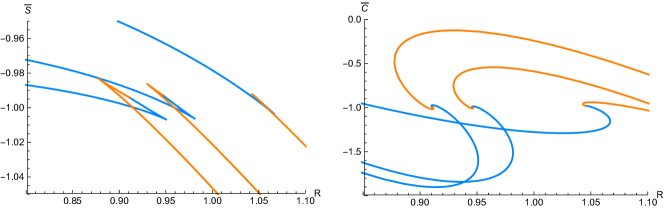
Figure 1: $\bar{S}$ (left) and $\bar{C}$ (right) as the functions of R for the gapped geometries with singular IR. In each pannel, there are three curves, which correspond to the different parameters $n=3.5$, $4.5$, $5.5$. As $n$ decreases, the multi-valued regions gradually shrink. Each curve includes two branches which have the disk topology (blue) and cylinder topology (orange), respectively. This color scheme is used in all the figures of the main text.

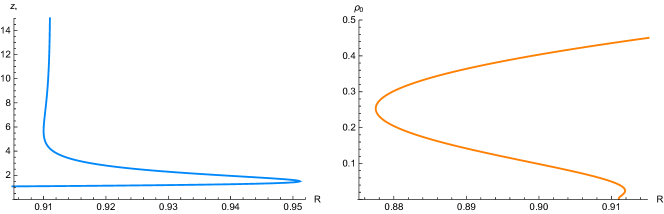
Figure 2: $z_{\ast}$ (left) and $\rho_{0}$ (right) as the functions of R for the gapped geometries with singular IR and $n=5.5$.

3 AdS Soliton

Consider the $\mathcal{N}=4$ super Yang-Mills theory in four dimensions, with one compactified spatial direction $\phi$. Suppose that $\phi$ is anti-periodic, which indicates massive fermions. At low energies, this theory is reduced to the three-dimensional gauge theory, associated with the confinement, mass gap and finite correlation length. By holography, it is dual to the AdS₅ soliton in IIB string theory [33]. The AdS soliton is a gapped geometry since its compact dimension shrinks to zero at some finite value of AdS radius, indicating an IR fixed point of the field theory at finite energy scale.

3.1 RT surface

We will study the soliton geometry

$$ds^{2}=\frac{{L^{2}}}{z^{2}}\left[\frac{dz^{2}}{h(z)}-dt^{2}+d\rho^{2}+\rho^{2}d\theta^{2}+h(z)d\phi^{2}\right]+L^{2}d\Omega_{5}^{2},$$ (24)

where

$$h(z)=1-(\frac{z}{z_{0}})^{4},$$ (25)

and $z_{0}$ is relevant to the period of $\phi$. Using the induced metric for the RT surface

$$ds_{\mathrm{ind}}^{2}=\frac{{L^{2}}}{z^{2}}\left[\left(\frac{1}{h}+\rho^{\prime 2}\right)dz^{2}+\rho^{2}d\theta^{2}+hd\phi^{2}\right]+L^{2}d\Omega_{5}^{2},$$ (26)

the entropy functional can be expressed as

$$\mathcal{S}=\frac{\pi\Omega_{5}L_{\phi}L^{8}}{2G_{N}}\int_{0}^{z_{0}}dz\frac{\rho}{z^{3}}\sqrt{1+h\rho^{\prime 2}},$$ (27)

where $\Omega_{5}$ is the unit volume of five-dimensional sphere, $L_{\phi}$ is the period of $\phi$, and $G_{N}$ is the ten-dimensional Newton constant. Variation of the entropy functional (27) with respect to $\rho(z)$ generates the EOM for the RT surface

$$\frac{d}{dz}\left(\frac{h\rho\rho^{\prime}}{z^{3}\sqrt{1+h\rho^{\prime 2}}}\right)=\frac{1}{z^{3}}\sqrt{1+h\rho^{\prime 2}}.$$ (28)

3.2 HEE and HSC

3.2.1 Large R expansion

In [24], it has been found that the RT surface is cylinder-like as R is large. Also, it has been noticed that the solution of the EOM (28) at large $\rho_{0}$ has the form

$$\rho(z)=\rho_{0}+\frac{1}{\rho_{0}}\rho_{1}(z)+\cdots,$$ (29)

where $\rho_{1}(z)$ should be vanishing in the IR ($z\rightarrow z_{0}$). Substituting this ansatz into (28), one can derive

$$\rho_{1}(z)=c_{2}+\frac{1-2c_{1}}{8}\log(1-z^{2})-\frac{1+2c_{1}}{8}\log(1+z^{2}),$$ (30)

where we have set $z_{0}=1$ for convenience. Noticing that the EOM (28) near $z=1$ has a solution

$$\rho=\rho_{0}+\frac{1-z}{4\rho_{0}}+\cdots,$$ (31)

the integral constants in (30) can be determined:

$$c_{1}=\frac{1}{2},\;c_{2}=\frac{\log 2}{4}.$$ (32)

Furthermore, we know $\rho(0)=R$, which imposes

$$\rho_{0}+\frac{1}{4\rho_{0}}\log(2)=R\text{.}$$ (33)

At large $\rho_{0}$, we have $\rho_{0}\simeq R$. Collecting all these results together, one can recast Eq. (29) as the solution at large R:

$$\rho(z)=R+\frac{1}{4R}\log(\frac{1}{1+z^{2}})+\cdots.$$ (34)

Then Eq. (27) can be expanded as

$$\mathcal{S}\sim R\int_{0}^{1}dz\frac{1}{z^{3}}+\frac{1}{R}\int_{0}^{1}dz\frac{1}{8z^{3}}\left[\frac{z^{2}h}{(1+z^{2})^{2}}+2\log(\frac{1}{1+z^{2}})\right]+\mathcal{O}(\frac{1}{R^{3}}),$$ (35)

where the TEE is vanishing. This is the essential result in [24]. Since one does not expect any long-range order in the ground state of (2+1) dimensional QCD, this result has been viewed as a consistency check on the HEE at that time.

Now we turn to study the HSC, which can be determined by

$$\mathcal{C=}\frac{\Omega_{5}L_{\phi}L^{8}}{4G_{N}}\int_{0}^{1}dz\frac{1}{z^{4}}\int_{0}^{\rho(z)}d\rho\rho.$$ (36)

Using the large-R expansion (34), we obtain

$$\mathcal{C}\sim R^{2}\int_{0}^{1}dz\frac{1}{z^{4}}+\int_{0}^{1}dz\frac{1}{2z^{4}}\log(\frac{1}{1+z^{2}})+\mathcal{O}(\frac{1}{R^{2}}).$$ (37)

There is no R-linear term.

3.2.2 Topology change

The IR boundary condition (31) can be used to solve numerically the RT surface with cylinder topology. For disk topology, we will look for the profile $z(\rho)$ of the RT surface, instead of $\rho(z)$. Rewrite the EOM (28) by $z(\rho)$, from which the IR boundary condition can be read:

$$z(\rho)=z_{\ast}+\frac{z_{\ast}h^{\prime}(z_{\ast})-6h(z_{\ast})}{8z_{\ast}}\rho^{2}+\cdots.$$ (38)

We also need the UV divergent terms of the HEE and HSC. In the UV $\left(z\rightarrow 0\right)$, the bulk geometry approaches AdS${}_{5}\times S^{5}$. The EOM (28) has the solution

$$\rho(z)=R-\frac{z^{2}}{4R}+\frac{z^{4}\log z}{32R^{3}}+\cdots.$$ (39)

Substituting it into Eq. (27) and Eq. (36), the divergent terms can be extracted:

$$\mathcal{S}_{\mathrm{div}}=\frac{\pi\Omega_{5}L_{\phi}L^{8}}{4G_{N}}\left(\frac{R}{\epsilon^{2}}+\frac{\log\epsilon}{4R}\right),\;\mathcal{C}_{\mathrm{div}}=\frac{\Omega_{5}L_{\phi}L^{8}}{4G_{N}}\left(\frac{R^{2}}{3\epsilon^{3}}-\frac{1}{2\epsilon}\right).$$ (40)

In the study of HEE [24], it has been shown that there is a ‘swallowtail’ phase transition associated with the topology change of the RT surface. In the left panel of Figure 3, we recover such a behavior. From the right panel in Figure 3, we have found that the HSC can probe the topology change in a different way: the complexity functional behaves as the ‘double-S’ instead of the ‘swallowtail’. The existence of the ‘double-S’ can be understood by the double and triple valued regions of the functions $z_{\ast}(R)$ and $\rho_{0}(R)$, see Figure 4.

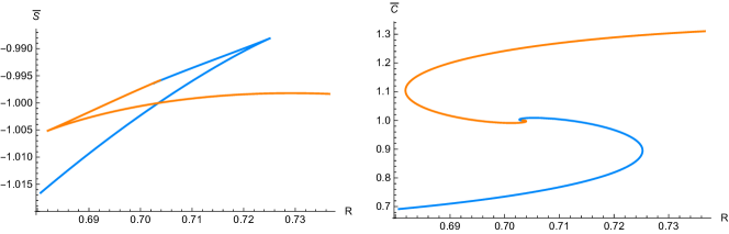
Figure 3: $\bar{S}$ (left) and $\bar{C}$ (right) as the functions of R for the AdS soliton.

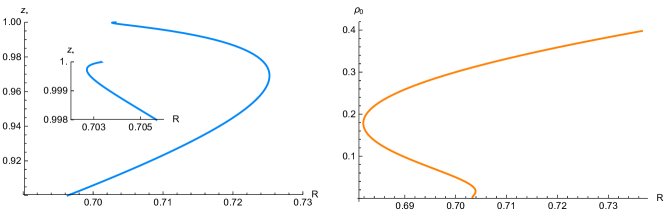
Figure 4: $z_{\ast}$ (left) and $\rho_{0}$ (right) as the functions of R for the AdS soliton.

It should be noted that our figure for the HEE is not exactly same as Figure 6 in [24]. This is because their HEE subtracts a term $\sim\left(\log R\right)/R$ besides the divergent terms. Moreover, the two functions $z_{\ast}(R)$ and $\rho_{0}(R)$ have been plotted in Figure 4 and Figure 5 of [24], respectively. Although the triple-valued region has not been noticed in their Figure 4, it is barely visible in their Figure 5.

4 Soft-wall model

The hard-wall and soft-wall models are both the bottom-up approaches to the AdS/QCD duality. A basic feature of hard-wall models is the existence of an IR brane at which the warped dimension abruptly ends. The hard IR wall breaks the conformal symmetry and provides the simplest realization of the confinement [34]. In the soft-wall model, there is a smoothing of the IR wall by invoking a dilaton field, which correctly produces the Regge behavior of highly excited mesons [35]. Consider the power-law behavior of the dilaton $\phi(z)=(\mu z)^{\nu}$, where $\mu$ is the energy scale and $z$ is the conformal coordinate. By analyzing the eigenfunctions of bulk fields with such power-law dilaton, the Kaluza-Klein mass spectrum with large $n$ can be given by $m_{n}^{2}\sim\mu^{2}n^{2-2/\nu}$ [36]. For $\nu<1$, the spectrum is gapless. For $\nu=1$, the spectrum becomes gapped but is continuous above the gap. For $\nu>1$, the spectrum is gapped and discrete.

4.1 RT surface

Suppose that the soft-wall geometry is described by

$$ds^{2}=\frac{L^{2}a(z)}{z^{2}}(dz^{2}-dt^{2}+d\rho^{2}+\rho^{2}d\theta^{2}).$$ (41)

In the IR $\left(\mu z\gg 1\right)$ and UV $\left(\mu z\ll 1\right)$, the warp factor are

$$a_{\mathrm{IR}}(z)=e^{-(\mu z)^{\nu}},\;a_{\mathrm{UV}}(z)=1.$$ (42)

Following [28], we will be interested in an explicit example

$$a(z)=\frac{1}{\cosh(\sqrt{(\mu z)^{2\nu}+1}-1},$$ (43)

which satisfies both boundary conditions. In Ref. [37], the dynamical soft-wall model with the warp factor $a(z)=e^{-(\mu z)^{\nu}}$ has been constructed. Now we are expecting that the warp factor (43) could be produced dynamically by a similar method. Note that the function (43) is flatter than $e^{-(\mu z)^{\nu}}$ in the UV. This is helpful to distinguish two space regions, namely Part (I) and Part (II), which will be introduced below. Hereafter, we set $\mu=1$ for convenience.

From Eq. (41), we write down the induced metric for the RT surface

$$ds_{\mathrm{ind}}^{2}=\frac{L^{2}a(z)}{z^{2}}\left[\left(1+\rho^{\prime 2}\right)dz^{2}+\rho^{2}d\theta^{2}\right],$$ (44)

which in turn gives the entropy functional

$$\mathcal{S}=\frac{\pi L^{2}}{2G_{N}}\int_{0}^{\infty}dz\frac{a\rho}{z^{2}}\sqrt{1+\rho^{\prime 2}}.$$ (45)

Taking the variation with respect to $\rho(z)$ derives the EOM for the RT surface

$$\frac{d}{dz}\left(\frac{a\rho}{z^{2}}\frac{\rho^{\prime}}{\sqrt{1+\rho^{\prime 2}}}\right)=\frac{a}{z^{2}}\sqrt{1+\rho^{\prime 2}}.$$ (46)

4.2 HEE and HSC

In [28], it has been shown that the RT surface only has the disk topology for $\nu<2$. Thus, the range $1\leq\nu<2$ is desired for the gapped geometry with a disk-like RT surface. Meanwhile, they proved that the TEE is vanishing by an analytical method. The basic strategy is to split the RT surface into three parts, see a schematic in Figure 1 of [28]. Part (I) is the deep UV region with $\epsilon<z<z_{c}^{(1)}$, where $z_{c}^{(1)}$ denotes the crossover scale at which the warp factor changes from $a_{\mathrm{UV}}(z)$ to $a_{\mathrm{IR}}(z)$. Part (II) is the intermediate region with $z_{c}^{(1)}<z<z_{c}^{(2)}$, and part (III) is the deep IR region with $z>z_{c}^{(2)}$. Here $z_{c}^{(2)}$ is chosen such that the surface area in part (II) is not exponentially suppressed by the warp factor $a_{\mathrm{IR}}(z)$ but will be in part (III). In part (I), the profile of the RT surface is known:

$$\rho(z)=R-\frac{z^{2}}{2R}+\mathcal{O}(\frac{1}{R^{2}}).$$ (47)

In part (II), it was found that

$$\rho(z)=\sqrt{2d_{1}}z_{0}^{1-\frac{\nu}{2}}-\frac{1}{\sqrt{2d_{1}}z_{0}^{1-\frac{\nu}{2}}}\frac{z^{2-\nu}}{\nu(2-\nu)}+\mathcal{O}(\frac{1}{z_{0}^{3-\frac{3\nu}{2}}}),$$ (48)

where $d_{1}$ is an integration constant. The parameter $z_{0}$ is required to obey $z\ll z_{0}$. By identifying $R=\sqrt{2d_{1}}z_{0}^{1-\frac{\nu}{2}}$, Eq. (48) is changed to

$$\rho(z)=R-\frac{1}{R}\rho_{\mathrm{II}}(z)+\mathcal{O}(\frac{1}{R^{3}}),$$ (49)

where

$$\rho_{\mathrm{II}}(z)=\frac{z^{2-\nu}}{\nu(2-\nu)}.$$ (50)

Thus, the RT surface in parts (I) and (II) can be taken together as

$$\rho(z)=R-\frac{\rho_{\mathrm{int}}(z)}{R}+\mathcal{O}(\frac{1}{R^{2}}),$$ (51)

where $\rho_{\mathrm{int}}(z)$ is an interpolating function.

Inserting Eq. (51) into Eq. (45), one can obtain

$$\mathcal{S}=\mathcal{S}_{\mathrm{I}}+\mathcal{S}_{\mathrm{II}}+\mathcal{S}_{\mathrm{III}},$$ (52)

where

$$\mathcal{S}_{\mathrm{I}}\sim R\int_{\epsilon}^{z_{c}^{(1)}}dz\frac{1}{z^{2}},$$ (53)

hence leading to a typical UV divergence, the interesting part is

$$\mathcal{S}_{\mathrm{II}}\sim R\int_{z_{c}^{(1)}}^{z_{c}^{(2)}}dz\frac{a_{\mathrm{IR}}}{z^{2}}+\frac{1}{R}\int_{z_{c}^{(1)}}^{z_{c}^{(2)}}dz\frac{a_{\mathrm{IR}}}{z^{2}}(\frac{\rho_{\mathrm{II}}^{\prime 2}}{2}-\rho_{\mathrm{II}})+\mathcal{O}(\frac{1}{R^{2}}),$$ (54)

and $\mathcal{S}_{\mathrm{III}}$ is exponentially suppressed by construction. Thus, the TEE is equal to zero.

We can study the HSC in a similar way. The only thing to be careful is that $z_{c}^{(2)}$ should be large enough to exponentially suppress the RT volume inside part (III) and $z_{0}$ (thereby R) should be so large that one has $z\ll z_{0}$ in part (II). Let’s consider the complexity functional

$$\mathcal{C}=\frac{L^{2}}{4G_{N}}\int_{0}^{\infty}dz\frac{a^{3/2}}{z^{3}}\int_{0}^{\rho(z)}d\rho\rho.$$ (55)

Using the large-R expansion (51), we read

$$\mathcal{C}=\mathcal{C}_{\mathrm{I}}+\mathcal{C}_{\mathrm{II}}+\mathcal{C}_{\mathrm{III}},$$ (56)

where the UV divergence comes from

$$\mathcal{C}_{\mathrm{I}}\sim\int_{\epsilon}^{z_{c}^{(1)}}dz\frac{R^{2}-z^{2}}{z^{3}},$$ (57)

the interesting part is

$$\mathcal{C}_{\mathrm{II}}\sim R^{2}\int_{z_{c}^{(1)}}^{z_{c}^{(2)}}dz\frac{a_{\mathrm{IR}}^{3/2}}{z^{3}}-2\int_{z_{c}^{(1)}}^{z_{c}^{(2)}}dz\frac{a_{\mathrm{IR}}^{3/2}}{z^{3}}\rho_{\mathrm{II}}+\mathcal{O}(\frac{1}{R}),$$ (58)

and $\mathcal{C}_{\mathrm{III}}$ is exponentially suppressed. One can see that the R-linear term disappears.

In this paper, the absence of the R-linear term is mainly exhibited by analytical methods. However, we have checked by numerical methods that this is true for all the models. As an example, we will numerically calculate the large-R behavior of HEE and HSC in the soft-wall model. Rewrite the EOM (46) by the profile $z(\rho)$, which can be solved using the IR boundary condition

$$z(\rho)=z_{\ast}+\frac{z_{\ast}a^{\prime}(z_{\ast})-2a(z_{\ast})}{4z_{\ast}a(z_{\ast})}\rho^{2}+\cdots.$$ (59)

Then we use the functions $b_{1}R+b_{2}/R$ and $b_{1}R^{2}+b_{2}$ to fit the large-R regions of $\bar{S}$ and $\bar{C}$, respectively. The result is shown in Figure 5.

One might wonder whether the numerical parameters $b_{1}$ and $b_{2}$ match their analytical expressions. For the previous two models, we find that they match perfectly. Take the HEE of AdS soliton as an example. The error is less than 0.01% for $R\simeq 20$. For the soft-wall model, however, the accuracy is limited since $z_{c}^{(1)}$ cannot be fixed accurately by its definition and $a(z)$ and $\rho(z)$ are discontinuous between (I) and (II). In fact, that is why we select to display the numerical result of the soft-wall model. To be clear, let’s compare the analytical expression of HEE to the numerical result. The behavior of HSC is similar. From Eq. (53) and Eq. (54), we have

$$\mathcal{S}_{\mathrm{I}}+\mathcal{S}_{\mathrm{II}} \sim R\int_{\epsilon}^{z_{c}^{(1)}}dz\frac{1}{z^{2}}+R\int_{z_{c}^{(1)}}^{z_{c}^{(2)}}dz\frac{a_{\mathrm{IR}}}{z^{2}}+\frac{1}{R}\int_{z_{c}^{(1)}}^{z_{c}^{(2)}}dz\frac{a_{\mathrm{IR}}}{z^{2}}(\frac{\rho_{\mathrm{II}}^{\prime 2}}{2}-\rho_{\mathrm{II}})+\mathcal{O}(\frac{1}{R^{2}})$$ (60)

$$= R\left(\frac{1}{\epsilon}+B_{1}\right)+\frac{1}{R}B_{2}+\mathcal{O}(\frac{1}{R^{2}}),$$

where

$$B_{1}=-\frac{1}{z_{c}^{(1)}}+\int_{z_{c}^{(1)}}^{z_{c}^{(2)}}dz\frac{a_{\mathrm{IR}}}{z^{2}},\;B_{2}=\int_{z_{c}^{(1)}}^{z_{c}^{(2)}}dz\frac{a_{\mathrm{IR}}}{z^{2}}(\frac{\rho_{\mathrm{II}}^{\prime 2}}{2}-\rho_{\mathrm{II}}).$$ (61)

We denote $\bar{b}_{1}$ and $\bar{b}_{2}$ as the rescaled parameters of $B_{1}$ and $B_{2}$, respectively. Following [28], we set $z_{c}^{(1)}=1$ and $z_{c}^{(2)}=\infty$. At $R\simeq 20$, we find $\bar{b}_{1}\simeq 1.4b_{1}$ and $\bar{b}_{2}\simeq 0.55b_{2}$. Thus, although the analytical expression of HEE does not match the numerical result very well, it does correctly reflect the fact that the TEE disappears.

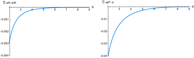
Figure 5: The large-R behavior of HEE (left) and HSC (right) in the soft-wall model. Here $b_{1}$ and $b_{2}$ are the best fitting parameters.

5 Holographic FQH effect

The FQH effect is associated with a state of quantum fluids that is dominated by strongly correlated electrons in high magnetic field. Due to the strong interaction and unusual symmetry in essence that can be implemented relatively easy in the holographic framework, it has been argued that the FQH system is likely to be a profitable place to apply the AdS/CFT correspondence [38]. Of particular interest to us, the FQH system is the prototype of topologically ordered medium that can be experimentally realized [39]. It has been found that the TEE in the fermionic Laughlin states is related to the filling fraction [40]. Thus, it would be interesting to study the HEE and HSC in holographic FQH states. Early holographic researches based on either bottom-up phenomenological approaches or top-down string/brane settings are very fruitful, e.g., see [41, 42, 43, 44, 45, 46, 47, 48, 49, 50, 51].

Here we will focus on a recent bottom-up model [52]. It is an Einstein-Maxwell-Axion-Dilaton theory with the SL(2,Z) symmetry, which not only captures the modular duality among various FQH states but also has the solution with the hard mass gap and correct Hall conductivity related to the filling fraction. Apparently, the solution to model FQH states should have both electric and magnetic charges. But ascribed to the SL(2,Z) transformation, it can be generated from a solution with purely electric charge. In Appendix A, we will review briefly how to numerically construct the electric solution that is a RG flow from the UV fixed point to the dilatonic scaling IR.

5.1 RT surface

Consider the solution in terms of the metric ansatz

$$ds^{2}=e^{2A(r)}\left[-f(r)dt^{2}+d\rho^{2}+\rho^{2}d\theta^{2}\right]+\frac{dr^{2}}{f(r)}.$$ (62)

The numerical functions of $f(r)$ and $A(r)$ are plotted in Appendix A, see Figure 7. The induced metric for the RT surface is

$$ds_{\mathrm{ind}}^{2}=\left(e^{2A}\rho^{\prime 2}+\frac{1}{f}\right)dr^{2}+e^{2A}\rho^{2}d\theta^{2},$$ (63)

from which the entropy functional can be expressed as

$$\mathcal{S}=\frac{\pi}{2G_{N}}\int_{0}^{\infty}dre^{A}\rho\sqrt{e^{2A}\rho^{\prime 2}+\frac{1}{f}}.$$ (64)

Taking the variation with respect to $\rho(r)$, one can derive the EOM for the RT surface

$$\frac{d}{dr}\frac{e^{3A}\rho\rho^{\prime}}{\sqrt{e^{2A}\rho^{\prime 2}+\frac{1}{f}}}=e^{A}\sqrt{e^{2A}\rho^{\prime 2}+\frac{1}{f}}.$$ (65)

5.2 HEE and HSC

5.2.1 Large R expansion

The IR metric is characterized by Eq. (102) and Eq. (103), with some parameters. By coordinate transformations, it can be rewritten as

$$ds^{2}=\frac{L^{2}}{z^{2}}\left(\frac{1}{az^{n}}dz^{2}-dt^{2}+d\rho^{2}+\rho^{2}d\theta^{2}\right),$$ (66)

where

$$n = \frac{4s}{s+1},$$ (67)

$$a = -\frac{256\gamma^{4}\Lambda L^{2-n}}{c^{2}\left(n-4\right)^{4}u\omega}\exp(nA_{\mathrm{IR}}-\frac{n}{n-4}\gamma\phi_{\mathrm{IR}}).$$ (68)

Note that the singular behavior of Eq. (68) at $n=4$ is forbidden due to the definition (67).

From Eq. (66), the holographic FQH model can be viewed as a concrete realization of the general geometries that studied in Sec. 2. To go ahead, we need to specify the parameter $n$. Consider the allowed region of parameters $s$ and $\gamma$. It is tiny since a sensible theory is required to satisfy five constraints, such as the absence of naked singularities at finite temperatures and the presence of mass gap, see Sec. 3.2 and Figure 2 in [52]. Then one can read that the minimum value of $n$ is 2 when $s=1$ [28]. In terms of Sec. 2, we infer that the TEE is vanishing and the HSC does not have the R-linear term. In other words, the absence of the constant term in the HEE and the R-linear term in the HSC depends on the geometry in the IR. Nevertheless, we have made double check of the large-R behavior by numerical methods, for which the complete background is needed.

5.2.2 Topology change

Following [52], we choose the parameters

$$\gamma=-0.85,\;s=1.2$$ (69)

which indicates the IR index $n=24/11>2$. Thus, the topology of the RT surface should change from disk to cylinder as R increases. Using the IR solutions (102)-(106), two kinds of the IR boundary conditions of the RT surface can be derived from the EOM (65) and its variant. They are

$$r(\rho) = r_{\ast}+\frac{1}{2}e^{2A(r_{\ast})}f(r_{\ast})A^{\prime}(r_{\ast})\rho^{2}+\cdots,\;\text{disk,}$$ (70)

$$\rho(r) = \rho_{0}+\frac{v_{1}}{\rho_{0}}\left[p\left(r-r_{0}\right)\right]^{v_{2}}+\cdots,\;\text{cylinder,}$$ (71)

where

$$v_{1}=-\frac{c^{2}u\omega\left(n-4\right)^{2}}{128\left(n^{2}-4\right)\gamma^{4}\Lambda}\exp(-2A_{\mathrm{IR}}+\frac{n}{n-4}\gamma\phi_{\mathrm{IR}}),\;v_{2}=4\gamma^{2}\frac{n-2}{\left(n-4\right)^{2}}.$$ (72)

We need to write down the HSC

$$\mathcal{C}=\frac{1}{4G_{N}L}\int_{0}^{\infty}dr\frac{e^{2A}}{\sqrt{f}}\int_{0}^{\rho(r)}d\rho\rho.$$ (73)

Using the solution in the UV

$$r(\rho)=-\frac{L}{2}\log\frac{R^{2}-\rho^{2}}{L^{2}},$$ (74)

we isolate the UV divergences in the HEE and HSC, which is

$$\mathcal{S}_{\mathrm{div}}=\frac{\pi L^{2}}{2G_{N}}\left(\frac{R}{L}e^{\frac{r_{\mathrm{inf}}}{L}}\right),\;\mathcal{C}_{\mathrm{div}}=\frac{L^{2}}{8G_{N}}\left[\frac{1}{2}\left(\frac{R}{L}e^{\frac{r_{\mathrm{inf}}}{L}}\right)^{2}-\frac{r_{\mathrm{inf}}}{L}\right],$$ (75)

where $r_{\mathrm{inf}}$ is the UV cutoff. Note that the UV divergences (75) are the same as those in pure AdS. In fact, Eq. (75) can be derived from Eq. (21) by a coordinate transformation $r=-L\log\frac{z}{L}$.

Collecting these results together and using the metric constructed in Appendix A, we can numerically calculate the HEE and HSC, see Figure 6. One can find that there is no obvious signal indicating the topology change of the RT surface. This might be relevant to the fact that the IR index $n$ is close to $2$, at which only the disk topology exists.

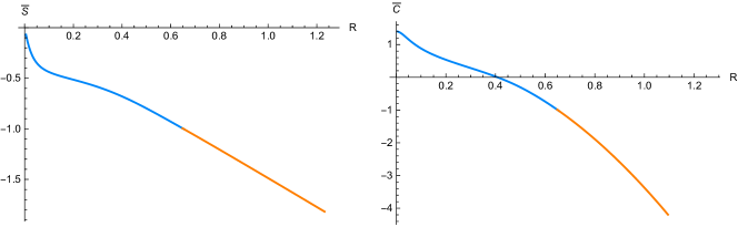
Figure 6: $\bar{S}$ (left) and $\bar{C}$ (right) as the functions of R for the FQH model.

6 Gauss-Bonnet curvature

TEE is the logarithm of the total quantum dimension. For FQH states, it can be calculated by the Chern-Simons theory [56]. For theories compactified on a higher genus surface, the TEE is related to the degeneracy of the ground state. In [28], a similar relation has been exhibited in holography, for which both the TEE and ground state degeneracy are produced by the GB curvature in the bulk. This holographic mechanism requires two conditions: i) the RT surface is disk-like; ii) the TEE is suppressed, except the GB contribution. Both of them have been realized in the soft-wall model that we studied in Sec. 4. Here we will study the GB contribution to the HSC in the same model.

It is implicitly assumed that the previous definition of the HSC (16) is applicable only to the Einstein gravity. Motivated by the Wald entropy [57], the HSC of a higher-derivative gravity theory was proposed [8]:

$$\mathcal{C=}\frac{1}{L}\int_{\mathcal{B}}\sqrt{\sigma}d^{3}xE^{\mu\nu\lambda\rho}\epsilon_{\mu\nu}\epsilon_{\lambda\rho},\;E^{\mu\nu\lambda\rho}=\frac{\partial\mathcal{L}}{\partial R_{\mu\nu\lambda\rho}}.$$ (76)

Here $\mathcal{L}$ is Lagrangian, $\mathcal{B}$ is the bulk space enclosed by the RT surface, $\sigma$ is the determinant of the space, and $\epsilon_{\mu\nu}$ should be certain binormal. As pointed out in [58], however, such definition suffers from the arbitrariness of the foliation in $\mathcal{B}$. Nevertheless, it was speculated that the complexity functional in high-derivative theories should involve contractions of the 4-rank tensor $E^{\mu\nu\lambda\rho}$ and the geometric quantities characterizing $\mathcal{B}$. As a result, a general complexity functional involving $E^{\mu\nu\lambda\rho}$ at most once was presented:

$$\mathcal{C}\mathcal{=}\frac{1}{L}\int_{\mathcal{B}}\sqrt{\sigma}d^{3}xE^{\mu\nu\lambda\rho}\left[\left(\beta_{1}n_{\mu}h_{\nu\lambda}n_{\rho}+\beta_{2}h_{\mu\rho}h_{\nu\lambda}\right)+\beta_{3}\right],$$ (77)

where $h_{\mu\nu}$ and $n_{\mu}$ are the induced metric and the normal vector of the space $\mathcal{B}$, respectively. The constants ($\beta_{1},\beta_{2},\beta_{3}$) are constrained so that the total functional is reduced to the volume functional for the Einstein gravity. Note that the complexity of higher-derivative gravity theories based on both CA and CV conjectures has been discussed in [59]. In the following, we will study Eq. (77).

For our aim, we split Eq. (77) into

$$\mathcal{C}\mathcal{=\mathcal{C}_{\mathrm{E}}+C}_{\mathrm{GB}},$$ (78)

where $\mathcal{\mathcal{C}_{\mathrm{E}}}$ depends only on the Einstein gravity and $\mathcal{C}_{\mathrm{GB}}$ denotes the GB correction. Importantly, in the 4-dimensional theory of gravity that we are concerning, the GB curvature contributes only a topological term to the gravity action and HEE [28]. Therefore, neither the spacetime metric nor the RT surface would be changed. Since we have shown in Sec. 4 that there is no R-linear term in $\mathcal{\mathcal{C}_{\mathrm{E}}}$, we only need to focus on $\mathcal{C}_{\mathrm{GB}}$.

Let’s write down the GB part of the Lagrangian

$$\mathcal{L}_{\mathrm{GB}}=\frac{\alpha}{16\pi G_{N}}(R_{\mu\nu\lambda\rho}R^{\mu\nu\lambda\rho}+R^{2}-4R_{\mu\nu}R^{\mu\nu}),$$ (79)

where $\alpha$ is the GB coupling. Accordingly, the 4-rank tensor is

$$E_{\mathrm{GB}}^{\mu\nu\lambda\rho} = \frac{\alpha}{16\pi G_{N}}{\Big{[}}2R^{\mu\nu\lambda\rho}+\left(g^{\mu\lambda}g^{\nu\rho}-g^{\mu\rho}g^{\nu\lambda}\right)R$$ (80)

$$+2\left(g^{\nu\lambda}R^{\mu\rho}-g^{\mu\lambda}R^{\nu\rho}+g^{\mu\rho}R^{\nu\lambda}-g^{\nu\rho}R^{\mu\lambda}\right){\Big{]}.}$$

Then $\mathcal{C}_{\mathrm{GB}}$ can be written as

$$\mathcal{C}_{\mathrm{GB}} \mathcal{=} \mathcal{C}_{1}+\mathcal{C}_{2},$$ (81)

$$\mathcal{C}_{1} = \frac{\beta_{1}}{L}\int_{\mathcal{B}}\sqrt{\sigma}d^{3}xE_{\mathrm{GB}}^{\mu\nu\lambda\rho}n_{\mu}h_{\nu\lambda}n_{\rho},$$ (82)

$$\mathcal{C}_{2} = \frac{\beta_{2}}{L}\int_{\mathcal{B}}\sqrt{\sigma}d^{3}xE_{\mathrm{GB}}^{\mu\nu\lambda\rho}h_{\mu\rho}h_{\nu\lambda}.$$ (83)

Using the metric (41) for the soft-wall model and the 4-rank tensor (80), one can calculate Eq. (82) and Eq. (83):

$$\mathcal{C}_{1} = \frac{\alpha\beta_{1}}{8G_{N}}\int_{0}^{\infty}dz\chi_{1}\frac{a^{3/2}}{z^{3}}\int_{0}^{\rho(z)}d\rho\rho,$$ (84)

$$\mathcal{C}_{2} = \frac{\alpha\beta_{2}}{8G_{N}}\int_{0}^{\infty}dz\chi_{2}\frac{a^{3/2}}{z^{3}}\int_{0}^{\rho(z)}d\rho\rho,$$ (85)

where

$$\chi_{1} = -\frac{6}{a}+\frac{2za^{\prime}}{a^{2}}+\frac{3z^{2}a^{\prime 2}}{2a^{3}}-\frac{2z^{2}a^{\prime\prime}}{a^{2}},$$ (86)

$$\chi_{2} = \frac{12}{a}-\frac{8za^{\prime}}{a^{2}}+\frac{2z^{2}a^{\prime\prime}}{a^{2}}.$$ (87)

To carry these integrals, the profile $\rho(z)$ obtained in Sec. 4 can be used. So let’s use the large-R expansion (51) and rewrite Eq. (84) and Eq. (85) as

$$\mathcal{C}_{i}=\mathcal{C}_{i,\mathrm{I}}+\mathcal{C}_{i,\mathrm{II}}+\mathcal{C}_{i,\mathrm{III}},\;i=1,2,$$ (88)

where

$$\mathcal{C}_{i,\mathrm{I}}\sim\int_{\epsilon}^{z_{c}^{(1)}}dz\frac{R^{2}-z^{2}}{z^{3}},$$ (89)

$$\mathcal{C}_{i,\mathrm{II}}\sim R^{2}\int_{z_{c}^{(1)}}^{z_{c}^{(2)}}dz\chi_{i}\frac{a^{3/2}}{z^{3}}-2\int_{z_{c}^{(1)}}^{z_{c}^{(2)}}dz\chi_{i}\frac{a^{3/2}}{z^{3}}\rho_{1}+\mathcal{O}(\frac{1}{R}),$$ (90)

and $\mathcal{C}_{i,\mathrm{III}}$ is exponentially suppressed by a suitable selection of $z_{c}^{(2)}$. One can see that there is no R-linear term in $\mathcal{C}_{\mathrm{GB}}$.

7 Conclusion

Using the gauge/gravity duality, we studied the complexity of the disk subregion in various (2+1)-dimensional gapped systems. We compared the HSC and the HEE from two aspects.

Firstly, we found that the R-linear term in the HSC is absent in the large-R expansion. In particular, it disappears for the similar reason that the TEE disappears in the HEE. This simple but interesting result suggests that there might be an underlying relation between the HSC and the topological order. However, we further showed that the GB curvature in the soft-wall model cannot produce the R-linear term in the HSC. If the R-linear term in the HSC is really correlated to the TEE, it would be needed to refine the present conjecture for the HSC in the GB gravity. In Appendix B, we will make some speculations on what the expected expression would look like.

Secondly, when the entanglement entropy probes the classic ‘swallowtail’ phase transition, the complexity is associated with a novel ‘double-S’ behavior. Our result supports to take the HSC as a good order parameter for some phase transitions [12, 13, 14]. However, neither the HEE nor the HSC can obviously exhibit the topology change of the RT surface in the holographic FQH model [52]. More sensitive order parameter might be required. Moreover, we have shown that the complexity can be more sensitive than the entanglement entropy to probe the topology change of the RT surface. Interestingly, a similar result also appeared in a recent work: by quantifying the complexity of subregions via their purification, it was demonstrated that the complexity can perceive some features insensitive to the entanglement entropy [60].

In the future, it may be worth studying the HSC through the tensor network. Among others [61, 62, 63, 64, 65], this direction is motivated by the following work. In [66], by comparing the minimal surfaces in the AdS soliton and the MERA (multi-scale entanglement renormalization ansatz) network [67], it was argued that the IR fixed-point state is the product state, which is consistent with the vanishing TEE. In [20], using the AdS₃/CFT₂ duality, it was found that the subregion complexity exhibits a topological discontinuity as the RT surface changes the configuration. Similar results have also been obtained using the CFT and the random tensor network [68]. It would be interesting to explore whether the vanishing R-linear term in the HSC could be reinterpreted by the tensor network. Moreover, by using the kinematic space as a bridge, it was pointed out recently that the HSC of a pure state can be represented by the HEE alone. Even for the excited states they considered, a part of the HSC can be determined by the HEE [73]. This paves a way to clarify the relation between the HEE and the HSC in the field theory. In particular, along this line, it would be promising to identify what are the counterparts of the TEE and the ‘swallowtail’ in the HSC. Our results should be useful in this regard.

Appendix A Numerical solution of the FQH model

We will study the Einstein-Maxwell-Axion-Dilation theory with the SL(2,Z) invariance:

$$S = \frac{1}{16\pi G_{N}}\int d^{4}x\sqrt{-g}\left(L_{g}+L_{F}+V\right),$$ (91)

$$L_{g} = R-\frac{1}{2}(\partial\phi)^{2}-\frac{1}{2}\frac{e^{-2\gamma\phi}}{\gamma^{2}}(\partial\tau_{1})^{2},$$ (92)

$$L_{F} = -\frac{1}{4}\left(e^{\gamma\phi}F^{2}+\frac{\tau_{1}}{2}\epsilon^{\mu\nu\rho\sigma}F_{\mu\nu}F_{\rho\sigma}\right),$$ (93)

$$V = \sum_{m,n\in Z}^{\prime}\left(\frac{|m+n\tau|^{2}}{\tau_{2}}\right)^{-s},$$ (94)

where $\tau=\tau_{1}+i\tau_{2}$ and $\tau_{2}=e^{\gamma\phi}$. The prime above $\sum$ stands for $m,n\neq 0$. With the ansatz for the metric

$$ds^{2}=e^{2A(r)}\left[-f(r)dt^{2}+dx^{2}+dy^{2}\right]+\frac{dr^{2}}{f(r)}$$ (95)

and the nonvanishing component of the gauge potential $A_{t}(r)$, one can derive five field equations

$$\tau_{2}^{\prime 2}+4\gamma^{2}\tau_{2}^{2}A^{\prime\prime}+\tau_{1}^{\prime 2} = 0,$$ (96)

$$f^{\prime\prime}+3A^{\prime}f^{\prime}-e^{-4A}\frac{q^{2}}{\tau_{2}} = 0,$$ (97)

$$\tau_{1}^{\prime\prime}+\left(3A^{\prime}+\frac{f^{\prime}}{f}-2\frac{\tau_{2}^{\prime}}{\tau_{2}}\right)\tau_{1}^{\prime}+\frac{\gamma^{2}\tau_{2}^{2}}{f}\frac{\partial V}{\partial\tau_{1}} = 0,$$ (98)

$$\left(\log\tau_{2}\right)^{\prime\prime}+\left(3A^{\prime}+\frac{f^{\prime}}{f}\right)(\log\tau_{2})^{\prime}+\frac{\tau_{1}^{\prime 2}}{\tau_{2}^{2}}+\frac{\gamma^{2}\tau_{2}}{f}\left(\frac{\partial V}{\partial\tau_{2}}+\frac{1}{2}e^{-4A}\frac{q^{2}}{\tau_{2}^{2}}\right) = 0,$$ (99)

$$-\frac{1}{2}\left(\frac{\tau_{2}^{2}}{\gamma\tau_{2}}\right)^{2}+6A^{\prime 2}+2A^{\prime}\frac{f^{\prime}}{f}-\frac{V}{f}+\frac{1}{2f}e^{-4A}\frac{q^{2}}{\tau_{2}^{2}} = 0.$$ (100)

The potential can be expanded for large $\tau_{2}$ as

$$V = 2\zeta(2s)\tau_{2}^{s}+2\sqrt{\pi}\tau_{2}^{1-s}\frac{\Gamma(s-1/2)}{\Gamma(s)}\zeta(2s-1)$$ (101)

$$+\frac{2\pi^{s}\sqrt{\tau_{2}}}{\Gamma(s)}\sum_{m,n\in Z}^{\prime}|\frac{m}{n}|^{s-1/2}K_{s-1/2}(2\pi\tau_{2}|mn|)e^{2i\pi mn\tau_{1}},$$

where $K$ denotes the modified Bessel function of the second kind. In the IR, it has the form $V=-2\Lambda\tau_{2}^{s}$, where $\Lambda=-\zeta(2s)$ and $s$ is a real parameter. It is found that there is an extremal scaling solution in the IR [52, 69]

$$A(r) = A_{\mathrm{IR}}+\frac{(\gamma-\delta)^{2}}{4}\log(p(r-r_{0})),$$ (102)

$$f(r) = \frac{-16\Lambda}{\omega uc^{2}}e^{-\delta\phi_{\mathrm{IR}}}(p(r-r_{0}))^{v},$$ (103)

$$\phi(r) = \phi_{\mathrm{IR}}+(\delta-\gamma)\log(p(r-r_{0})),$$ (104)

$$\tau_{1}(r) = a_{0},$$ (105)

$$A_{t}(r) = \frac{8}{\omega}\sqrt{\frac{v\Lambda}{u}}e^{-\frac{\gamma+\delta}{2}\phi_{\mathrm{IR}}}(p(r-r_{0}))^{\frac{\omega}{4}},$$ (106)

where $\omega=3\gamma^{2}-\delta^{2}-2\gamma\delta+4$, $u=\gamma^{2}-\gamma\delta+2$, $v=-\delta^{2}+\gamma\delta+2$, $\delta=-\gamma s$, and

$$q^{2}=e^{-4A_{\mathrm{IR}}}\frac{-4\Lambda e^{(\gamma-\delta)\phi_{\mathrm{IR}}}(2+\gamma\delta-\delta^{2})}{(2+\gamma^{2}-\gamma\delta)}\frac{p^{2}}{c^{2}}.$$ (107)

Following [52], we will explain how to construct a numerical solution of field equations. First, we will reduce two independent parameters: the parameter $\phi_{\mathrm{IR}}$ can be determined by Eq. (107) and one can infer $c=p$ from Eq. (99). Second, given six parameters $\left(\gamma,s,a_{0},p,q,r_{0}\right)$, we can use Eqs. (102)-(106) as the IR boundary conditions to obtain a trial solution, where the remained parameter $A_{\mathrm{IR}}$ is turned to respect $6A^{\prime 2}f=6/L^{2}$ in the UV. This is required by Eq. (100). Here $L=\sqrt{6/V(\tau_{\ast},\bar{\tau}_{\ast})}$ is the AdS radius and $\tau_{\ast}$ denotes certain UV fixed point. Third, the field equations are invariant under two transformations

$$r \rightarrow \lambda_{1}r,\;f\rightarrow\lambda_{1}^{2}f,$$ (108)

$$e^{A} \rightarrow \lambda_{2}e^{A},\;q\rightarrow\lambda_{2}^{2}q,$$ (109)

which have the parameters $\lambda_{i}$, $i=1,2$. In terms of these symmetries, one can rescale the trial solution to meet the UV boundary condition $f=1$ and $A=r/L$.

As an example, we will construct the trial solution by setting $\tau_{\ast}=e^{\frac{\pi i}{3}}$ and selecting the parameters

$$\gamma=-0.85,\;s=1.2,\;a_{0}=0.2,\;p=1,\;q=1,\;r_{0}=0.$$ (110)

The final metric functions are plotted in Figure 7.

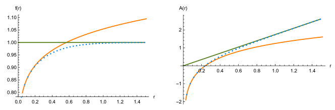
Figure 7: The metric functions $f(r)$ (left) and $A(r)$ (right) in the FQH model. They are dotted lines and coloured in blue. The orange line and the green line denote the IR and UV asymptotics, respectively.

Appendix B Gauss-Bonnet formula on three-dimensional manifolds

We further explore the HSC in the GB gravity. Since we suspect that Eq. (77) might need to be improved, a natural question is what the expected expression looks like.

Let’s write down the HEE in the GB gravity [70, 71, 72]

$$\mathcal{S}=\frac{1}{4G_{N}}\left[\int_{\Sigma}d^{2}x\sqrt{h}+\alpha\left(\int_{\Sigma}d^{2}x\sqrt{h}\;^{(2)}R+2\int_{\partial\Sigma}dx\sqrt{h_{\partial}}K\right)\right],$$ (111)

where $h$ is the determinant of the metric on the RT surface $\Sigma$, ${}^{(2)}R$ is the intrinsic Ricci scalar defined on $\Sigma$, $h_{\partial}$ is the determinant of induced metric on the boundary $\partial\Sigma$, and $K$ is the extrinsic curvature of the boundary. The terms in the parentheses are proportional to the Euler characteristic $\chi$ of the RT surface due to the GB theorem.

We turn to observe the proposals for the HSC in the GB gravity, see Eq. (76) and Eq. (77). They are mainly motivated by the expression of the HEE (or Wald entropy) in the higher-derivative theory. However, comparing them with Eq. (111), one can find an obvious difference: there are no topological features in Eq. (76) and Eq. (77). In view of this, a natural proposal for the HSC in the GB gravity would be to involve a topological invariant like the integral of the Euler density, but it should be defined on the three-dimensional space inside the RT surface. It is well-known that the even dimensionality is essential for the GB theorem. If the manifold is odd-dimensional, the Euler characteristic is zero. Interestingly, we notice that there is a formula in the odd-dimensional manifold which is actually related to the GB theorem [74]:

$$\frac{1}{l(\xi)}\frac{1}{2\pi}\left[\int_{M}\mathrm{K}dM+3\mathrm{Vol}(M)\right]=2\beta_{0}\left(M\right)-\beta_{1}\left(M\right),$$ (112)

where $M$ is a three-dimensional Sasakian manifold, $\xi$ is the regular unit Killing vector, $\mathrm{K}$ is the sectional curvature of the surface orthogonal to $\xi$, $l(\xi)$ is the length of its trajectory, and $\beta_{i}\left(M\right)$ denotes the i-th Betti number of $M$. In particular, the length scale seems to appear in a suitable place. However, the space inside the RT surface is not the Sasakian manifold in general. In the future, it would be interesting to investigate whether the restriction on the manifold could be sufficiently relaxed and $l(\xi)$ could be related to the size of entangling surface. We emphasize that this direction is presently quite speculative.

References

- [1] B. Swingle, Phys. Rev. D 86, 065007 (2012) [arXiv:0905.1317].
- [2] M. Van Raamsdonk, [arXiv:0907.2939].
- [3] S. Ryu and T. Takayanagi, Phys. Rev. Lett. 96, 181602 (2006) [arXiv:hep-th/0603001].
- [4] L. Susskind, [arXiv:1411.0690].
- [5] L. Susskind, [arXiv:1403.5695].
- [6] A. R. Brown, D. A. Roberts, L. Susskind, B. Swingle and Y. Zhao, Phys. Rev. Lett. 116, 191301 (2016) [arXiv:1509.07876].
- [7] M. Miyaji, T. Numasawa, N. Shiba, T. Takayanagi and K. Watanabe, Phys. Rev. Lett. 115, 261602 (2015) [arXiv:1507.07555].
- [8] M. Alishahiha, Phys. Rev. D 92, 126009 (2015) [arXiv:1509.06614].
- [9] O. Ben-Ami and D. Carmi, JHEP 1611, 129 (2016) [arXiv:1609.02514].
- [10] W. C. Gan and F. W. Shu, Phys. Rev. D 96, 026008 (2017) [arXiv:1702.07471].
- [11] S. Banerjee, J. Erdmenger and D. Sarkar, [arXiv:1701.02319].
- [12] D. Momeni, S. A. H. Mansoori and R. Myrzakulov, Phys. Lett. B 756, 354 (2016) [arXiv:1601.03011].
- [13] P. Roy and T. Sarkar, Phys. Rev. D 96, 026022 (2017) [arXiv:1701.05489].
- [14] M. K. Zangeneh, Y. C. Ong and B. Wang, Phys. Lett. B 771, 235 (2017) [arXiv:1704.00557].
- [15] D. Carmi, R. C. Myers and P. Rath, JHEP 1703 118 (2017) [arXiv:1612.00433]; D. Carmi, [arXiv:1709.10463].
- [16] D. Momeni, M. Faizal, K. Myrzakulov and R. Myrzakulov, Phys. Lett. B 765, 154 (2017) [arXiv:1604.06909]; D. Momeni, M. Faizal, A. Myrzakul, S. Bahamonde and R. Myrzakulov, Eur. Phys. J. C 77, 391 (2017) [arXiv:1608.08819]; N. S. Mazhari, D. Momeni, S. Bahamonde, M. Faizal and R. Myrzakulov, Phys. Lett. B 766, 94 (2017) [arXiv:1609.00250]; D. Momeni, M. Faizal, S. Bahamonde and R. Myrzakulov, Phys. Lett. B 762, 276 (2016) [arXiv:1610.01542]; D. Momeni, M. Faizal, S. Alsaleh, L. Alasfar, A. Myrzakul and R. Myrzakulov, [arXiv:1704.05785].
- [17] E. Bakhshaei, A. Mollabashi and A. Shirzad, Eur. Phys. J. C 77, 665 (2017) [arXiv:1703.03469].
- [18] S. Karara and S. Gangopadhyay, [arXiv:1711.10887].
- [19] B. Chen, W. M. Li, R. Q. Yang, C. Y. Zhang, and S. J. Zhang, [arXiv:1803.06680].
- [20] R. Abt, J. Erdmenger, H. Hinrichsen, C. M. Melby-Thompson, R. Meyer, C. Northe and I. A. Reyes, [arXiv:1710.01327].
- [21] A. Kitaev and J. Preskill, Phys. Rev. Lett. 96, 110404 (2006) [arXiv:hep-th/0510092].
- [22] M. Levin and X. G. Wen, Phys. Rev. Lett. 96, 110405 (2006).
- [23] T. Grover, A. M. Turner and A. Vishwanath, Phys. Rev. B 84, 195120 (2011).
- [24] A. Pakman and A. Parnachev, JHEP 0807, 097 (2008) [arXiv:0805.1891].
- [25] H. Liu and M. Mezei, JHEP 1304, 162 (2013) [arXiv:1202.2070].
- [26] H. Liu and M. Mezei, JHEP 1401, 098 (2014) [arXiv:1309.6935].
- [27] M. Fujita, W. Li, S. Ryu and T. Takayanagi, JHEP 0906, 066 (2009) [arXiv:0901.0924].
- [28] A. Parnachev and N. Poovuttikul, JHEP 1510, 92 (2015) [arXiv:1504.08244].
- [29] L. McGough and H. Verlinde, JHEP 1311, 208 (2013) [arXiv:1308.2342].
- [30] Z. X. Luo and H. Y. Sun, JHEP 1712, 116 (2017) [arXiv:1709.06066].
- [31] I. R. Klebanov, D. Kutasov and A. Murugan, Nucl. Phys. B 796, 274 (2008) [arXiv:0709.2140].
- [32] T.Nishioka and T. Takayanagi, JHEP 0701, 090 (2007) [arXiv:hep-th/0611035].
- [33] E. Witten, Adv. Theor. Math. Phys. 2, 505 (1998) [arXiv:hep-th/9803131].
- [34] J. Polchinski and M. J. Strassler, Phys. Rev. Lett. 88, 031601 (2002) [arXiv:hep-th/0109174].
- [35] A. Karch, E. Katz, D. T. Son and M. A. Stephanov, Phys. Rev. D 74, 015005 (2006) [arXiv:hep-ph/0602229].
- [36] B. Batell, T. Gherghetta and D. Sword, Phys. Rev. D 78, 116011 (2008) [arXiv:0808.3977].
- [37] B. Batell and T. Gherghetta, Phys. Rev. D 78, 026002 (2008) [arXiv:0801.4383].
- [38] A. Bayntun, C. P. Burgess, B. P. Dolan and S. S. Lee, New J. Phys. 13, 035012 (2011) [arXiv:1008.1917].
- [39] X. G. Wen and Q. Niu, Phys. Rev. B 41, 9377 (1990).
- [40] M. Haque, O. Zozulya and K. Schoutens, Phys. Rev. Lett. 98, 060401 (2007).
- [41] E. Keski-Vakkuri and P. Kraus, JHEP 0809, 130 (2008) [arXiv:0805.4643].
- [42] J. L. Davis, P. Kraus and A. Shah, JHEP 0811, 020 (2008) [arXiv:0809.1876].
- [43] M. Fujita, W. Li, S. Ryu and T. Takayanagi, JHEP 0906, 066 (2009) [arXiv:0901.0924].
- [44] Y. Hikida, W. Li and T. Takayanagi, JHEP 0907, 065 (2009) [arXiv:0903.2194].
- [45] J. Alanen, E. Keski-Vakkuri, P. Kraus and V. Suur-Uski, JHEP 0911, 014 (2009) [arXiv:0905.4538].
- [46] O. Bergman, N. Jokela, G. Lifschytz and M. Lippert, JHEP 1010, 063 (2010) [arXiv:1003.4965].
- [47] E. Gubankova, J. Brill, M. Cubrovic, K. Schalm, P. Schijven and J. Zaanen, Phys. Rev. D 84, 106003 (2011) [arXiv:1011.4051].
- [48] N. Jokela, G. Lifschytz and M. Lippert, JHEP 1102, 104 (2011) [arXiv:1012.1230].
- [49] M. Fujita, M. Kaminski and A. Karch, JHEP 1207, 150 (2012) [arXiv:1204.0012].
- [50] D. Melnikov, E. Orazi and P. Sodano, JHEP 1305, 116 (2013) [arXiv:1211.1416].
- [51] C. Kristjansen and G. W. Semenoff, JHEP 1306, 048 (2013) [arXiv:1212.5609].
- [52] M. Lippert, R. Meyer and A. Taliotis, JHEP 1501, 023 (2015) [arXiv:1409.1369].
- [53] B. P. Dolan, J. Phys. A 32, L243 (1999) [arXiv:cond-mat/9805171].
- [54] C. P. Burgess, R. Dib and B. P. Dolan, Phys. Rev. B 62, 15359 (2000) [arXiv:cond-mat/9911476].
- [55] C. P. Burgess and B. P. Dolan, Phys. Rev. B 65, 155323 (2002) [arXiv:cond-mat/0105621].
- [56] S. Dong, E. Fradkin, R. G. Leigh, and S. Nowling, JHEP 0805, 016 (2008) [arXiv:0802.3231].
- [57] R. M. Wald, Phys. Rev. D 48, 3427 (1993) [arXiv:gr-qc/9307038]; V. Iyer and R. M. Wald, Phys. Rev. D 50, 846 (1994) [arXiv:gr-qc/9403028].
- [58] P. Bueno, V. S. Min, A. J. Speranza and M. R. Visser, Phys. Rev. D 95, 0460033 (2017) [arXiv:1612.04374].
- [59] M. Alishahiha, A. F. Astaneh, A. Naseh, and M. H. Vahidinia, JHEP 1705, 009 (2017) [arXiv:1702.06796].
- [60] H. A. Camargo, P. Caputa, D. Das, M. P. Heller, and R. Jefferson arXiv:1807.07075.
- [61] H. Q. Zhou, R. Orus, and G. Vidal, Phys. Rev. Lett. 100, 080601 (2008) [arXiv:0709.4596].
- [62] D. Stanford and L. Susskind, Phys. Rev. D 90, 126007 (2014) [arXiv:1406.2678].
- [63] M. Miyaji, T. Takayanagi, PTEP 2015, 073B03 (2015) [arXiv:1503.03542].
- [64] P. Caputa, N. Kundu, M. Miyaji, T. Takayanagi, and K. Watanabe, Phys. Rev. Lett. 119, 071602 (2017) [arXiv:1703.00456]; JHEP 1711, 097 (2017) [arXiv:1706.07056].
- [65] B. Czech, Phys. Rev. Lett. 120, 031601 (2018) [arXiv:1706.00965].
- [66] M. Ishihara, F. L. Lin, and B. Ning, Nucl. Phys. B 872, 391 (2013) [arXiv:1203.6153].
- [67] B. Swingle, Phys. Rev. D 86, 065007 (2012) [arXiv:0905.1317]; G. Evenbly and G. Vidal, J. Stat. Phys. 145, 891 (2011) [arXiv:1106.1082]; G. Vidal, Phys. Rev. Lett. 98, 070201 (2007) [arXiv:cond-mat/0512165]; G. Vidal, Phys. Rev. Lett. 101, 110501 (2008) [arXiv:quant-ph/0610099]; G. Evenbly and G. Vidal, Phys. Rev. Lett. 115, 180405 (2015) [arXiv:1412.0732].
- [68] P. Hayden, S. Nezami, X. L. Qi, N. Thomas, M. Walter, and Z. Yang, JHEP 11, 009 (2016) [arXiv:1601.01694].
- [69] C. Charmousis, B. Gouteraux, B. S. Kim, E. Kiritsis and R. Meyer, JHEP 1011, 151 (2010) [arXiv:1005.4690].
- [70] D. V. Fursaev, JHEP 0609, 018 (2006) [arXiv:hep-th/0606184].
- [71] J. de Boer, M. Kulaxizi and A. Parnachev, JHEP 1107, 109 (2011) [arXiv:1101.5781].
- [72] L. Y. Hung, R. C. Myers and M. Smolkin, JHEP 1104, 025 (2011) [arXiv:1101.5813].
- [73] R. Abt, J. Erdmenger, M. Gerbershagen, C. M. Melby–Thompson, and C. Northe, arXiv:1805.10298.
- [74] S. Tanno, J. Math. Soc. Japan, 24, 204 (1972).
- [75] A. Reventós, Tohoku Math. J. (2) 31, 165 (1979).