Statistical test for fractional Brownian motion based on detrending moving average algorithm

Abstract

Motivated by contemporary and rich applications of anomalous diffusion processes we propose a new statistical test for fractional Brownian motion, which is one of the most popular models for anomalous diffusion systems. The test is based on detrending moving average statistic and its probability distribution. Using the theory of Gaussian quadratic forms we determined it as a generalized chi-squared distribution. The proposed test could be generalized for statistical testing of any centered non-degenerate Gaussian process. Finally, we examine the test via Monte Carlo simulations for two exemplary scenarios of subdiffusive and superdiffusive dynamics.

1 Introduction

The theory of stochastic processes is currently an important and developed branch of mathematics [10, 22, 25]. The key issue from the point of view of the application of stochastic processes is statistical inference for such random objects [41, 53, 62, 64]. This field consists of statistical methods for the reliable estimation, identification, and validation of stochastic models. Such a part of the theory of stochastic processes and the statistics developed for them are used to model phenomena studied by other fields such as physics [28, 60, 75], chemistry [28, 66, 75], biology [11, 14, 28, 32, 65, 66], engineering [7, 67], among others.

This work is motivated by growing interest and applications of the special class of stochastic processes, namely anomalous diffusion processes, which largely depart from the classical Brownian diffusion theory [50, 63]. Such processes are characterized by a nonlinear power-law growth of the mean squared displacement (MSD) in the course of time. Their anomalous diffusion behavior manifested by nonlinear MSD is intimately connected with the breakdown of the central limit theorem, caused by either broad distributions or long-range correlations. Today, the list of systems displaying anomalous dynamics is quite extensive [26, 31, 35, 44, 56, 59]. Therefore in recent years, there has been great progress in the understanding of the different mathematical models that can lead to anomalous diffusion [36, 37, 51]. One of the most popular of them is the fractional Brownian motion (FBM) [29, 33, 35, 42, 51, 73, 78]. Introduced by Kolmogorov [38] and studied by Mandelbrot in a series of papers [46, 47], it is now well-researched stochastic process. FBM is still constantly developed by mathematicians in different aspects [5, 23, 55, 57, 77].

The main subject considered in this work is the issue of rigorous and valid identification of the FBM model. The problem of FBM identification has been described in the mathematical literature for a long time [8, 18]. However, most of the works mainly concern various methods of estimating the parameters of the FBM model. They are based, among others, on p-variation [45], discrete variation [19], sample quantiles [20] and other methods [9, 12, 21, 27, 43, 52, 74, 81]. A certain gap in this theory is the lack of tools such as rigorous statistical tests to identify the FBM model in empirical data. Some approaches to FBM identification are known, e.g., application of empirical quantiles [13], distinguishing FBM from pure Brownian motion [40]. According to the author’s current knowledge, the only statistical test for the FBM model is the test based on the distribution of the time average MSD [71]. Due to the lack of statistical tests specially designed for the FBM model, in this work, we propose such a statistical testing procedure.

The proposed test has a test statistic which is the detrending moving average (DMA) statistic introduced in the paper [2]. For more than a decade, the DMA algorithm has become an important and promising tool for the analysis of stochastic signals. It is constantly developed and improved [4, 16, 17, 69], its multifractal version was created and used [15, 30, 34, 80] and it is applied for different empirical datasets [39, 58, 61, 68]. As one of the important method for fluctuation analysis, the DMA algorithm was often compared with other methods [6, 79, 82]

In section 2 we show that the distribution of the DMA statistics follows the generalized chi-squared distribution. The main section 3 demonstrates the statistical testing procedure based on computing the DMA statistic for empirical data. In section 4 the results of Monte Carlo simulations of the proposed test are presented and discussed. Section 5 contains conclusions and final remarks. In the last section 6, the Matlab code of the proposed test is presented.

2 Probability distribution of DMA statistic

The DMA algorithm was introduced in [2]. For a finite trajectory $\{X(1),X(2),\ldots,X(N)\}$ of a stochastic process the DMA statistic has the following form

$$\sigma^{2}(n)=\frac{1}{N-n}\sum_{j=n}^{N}(X(j)-\tilde{X}_{n}(j))^{2},\quad n=2,3,\ldots,N-1,$$ (1)

where $\tilde{X}_{n}(j)$ is a moving average of $n$ observations $X(j),\ldots,X(j-n+1)$, i.e.

$$\tilde{X}_{n}(j)=\frac{1}{n}\sum_{k=0}^{n-1}X(j-k).$$

The statistic $\sigma^{2}(n)$ is a random variable which computes the mean squared distance between the process $X(j)$ and its moving average $\tilde{X}_{n}(j)$ of the window size $n.$ It has scaling law behavior $\sigma^{2}(n)\sim C_{H}n^{2H},$ where $H$ is a self–similarity parameter of the signal [2, 4]. The constant $C_{H}$ has explicit expression computed in the case of fractional Brownian motion [4]. As a byproduct of this scaling law one can estimate the self–similarity parameter $H$ from linear fitting on double logarithmic scale [6, 17, 70].

In this work, we leave the issue of DMA algorithm as an estimation method and concentrate on the probability characteristics of this random statistic. Throughout the paper, we assume that the stochastic process $X(j)$ is a centered Gaussian process. Therefore a finite trajectory $\mathbb{X}=\{X(1),X(2),\ldots,X(N)\}$ is a centered Gaussian vector with covariance matrix $\Sigma=\{E\left[X(j)X(k)\right]:j,k=1,2,\ldots,N\}.$ Let introduce the process $Y(j):=X(j+n-1)-\tilde{X}_{n}(j+n-1),$ which is still a centered Gaussian process. We calculate the covariance matrix of the vector $\mathbb{Y}=\{Y(1),Y(2),\ldots,Y(N-n+1)\}$

$$E\left[Y(j)Y(k)\right] = E\left[X(j+n-1)X(k+n-1)\right]-E\left[X(j+n-1)\tilde{X}_{n}(k+n-1)\right]-E\left[\tilde{X}_{n}(j+n-1)X(k+n-1)\right]$$ (2)

$$+ E\left[\tilde{X}_{n}(j+n-1)\tilde{X}_{n}(k+n-1)\right]=E\left[X(j+n-1)X(k+n-1)\right]-\frac{1}{n}\sum_{m=k}^{k+n-1}E\left[X(j+n-1)X(m)\right]$$

$$- \frac{1}{n}\sum_{l=j}^{j+n-1}E\left[X(k+n-1)X(l)\right]+\frac{1}{n^{2}}\sum_{j\leq l\leq j+n-1}\sum_{k\leq m\leq k+n-1}E\left[X(l)X(m)\right].$$

That matrix we denote by $\tilde{\Sigma}=\{E\left[Y(j)Y(k)\right]:j,k=1,2,\ldots,N-n+1\}.$ We see that the dependence structure of the process $Y(i)$ is fully determined by the covariance of the process $X(i).$ Moreover the covariance $E\left[X(k)X(m)\right]$ in formula (2) has a prefactor

$$\left(1-\frac{1}{n}\right)^{2}, l=j+n-1\wedge m=k+n-1,$$ for

$$\frac{1}{n^{2}}-\frac{1}{n}, (l=j+n-1\wedge m\neq k+n-1)\vee(l\neq j+n-1\wedge m=k+n-1),$$ for

$$\frac{1}{n^{2}}, l\neq j+n-1\wedge m\neq k+n-1.$$ for

Therefore we can rewrite the formula (2) in the equivalent form

$$E\left[Y(j)Y(k)\right] = \left(1-\frac{1}{n}\right)^{2}E\left[X(j+n-1)X(k+n-1)\right]+\left(\frac{1}{n^{2}}-\frac{1}{n}\right)\left[\sum_{m=k}^{k+n-2}E\left[X(j+n-1)X(m)\right]\right.$$ (3)

$$+ \left.\sum_{l=j}^{j+n-2}E\left[X(l)X(k+n-1)\right]\right]+\frac{1}{n^{2}}\sum_{j\leq l\leq j+n-2}\sum_{k\leq m\leq k+n-2}E\left[X(l)X(m)\right].$$

The average value of random variable $\sigma^{2}(n)$ we can now express based on (2) and (3) by covariance structure of the process $X(j)$

$$E\left[\sigma^{2}(n)\right] = \frac{1}{N-n}\sum_{j=n}^{N}E\left[\left(X(j)-\tilde{X}_{n}(j)\right)^{2}\right]=\frac{1}{N-n}\sum_{j=n}^{N}E\left[Y^{2}(j-n+1)\right]$$ (4)

$$= \!\!\!\!\!\frac{1}{N-n}\sum_{j=n}^{N}\!\!\left\{\left(1-\frac{1}{n}\right)^{2}\!\!E[X^{2}(j)]+2\left(\frac{1}{n^{2}}-\frac{1}{n}\right)\!\!\sum_{m=j-n+1}^{i-1}\!\!\!\!E[X(j)X(m)]+\frac{1}{n^{2}}\!\!\sum_{j-n+1}^{j-1}\!E[X^{2}(m)]+\frac{2}{n^{2}}\!\!\!\sum_{j-n+1\leq k<m\leq j-1}\!\!\!\!\!\!\!\!E[X(m)X(l)]\right\}.$$

We can also express the variance of the random variable $\sigma^{2}(n)$

$$Var\left[\sigma^{2}(n)\right] = \frac{1}{(N-n)^{2}}Var\left[\sum_{j=n}^{N}Y^{2}(j-n+1)\right]=\frac{1}{(N-n)^{2}}\sum_{l,m=n}^{N}Cov\left(Y^{2}(l-n+1),Y^{2}(m-n+1)\right)$$ (5)

$$= \frac{1}{(N-n)^{2}}\sum_{l,m=n}^{N}E\left[Y^{2}(l-n+1)Y^{2}(m-n+1)\right]-E\left[Y^{2}(l-n+1)\right]E\left[Y^{2}(m-n+1)\right].$$

The terms $E\left[Y^{2}(l-n+1)\right]$ and $E\left[Y^{2}(m-n+1)\right]$ one can compute from covariance of the process $Y(j)$ according to (3). The 4th–order moment $E\left[Y^{2}(l-n+1)Y^{2}(m-n+1)\right]$ can be expressed by covariance structure of process $Y(j)$ according to Isserlis’ theorem [72]:

$$E\left[Y^{2}(l-n+1)Y^{2}(m-n+1)\right]=E\left[Y^{2}(l-n+1)\right]E\left[Y^{2}(m-n+1)\right]+2E\left[Y(l-n+1)Y(m-n+1)\right]^{2}.$$

Therefore applying above to (5) we get

$$Var\left[\sigma^{2}(n)\right]=\frac{2}{(N-n)^{2}}\sum_{l,m=n}^{N}E\left[Y(l-n+1)Y(m-n+1)\right]^{2}.$$ (6)

Using (3) one can present formula (6) for variance in terms of covariance structure of the underlying process $X(i).$

In order to describe more probabilistic properties of the random variable $\sigma^{2}(n)$ we notice the quadratic form representation

$$\sigma^{2}(n)=\frac{1}{N-n}\sum_{j=n}^{N}Y^{2}(j-n+1)=\frac{1}{N-n}\mathbb{Y}\mathbb{Y}^{T},$$

where $\mathbb{Y}^{T}$ is a vertical vector which is a transpose of the vector $\mathbb{Y}.$ The random object $\mathbb{Y}\mathbb{Y}^{T}$ is a quadratic form of a Gaussian vector $\mathbb{Y}.$ Therefore we apply the theory of Gaussian quadratic forms to study random variable $(N-n)\sigma^{2}(n).$ The theory of Gaussian quadratic forms [49] provides us with the following representation

$$(N-n)\sigma^{2}(n)\stackrel{{\scriptstyle d}}{{=}}\sum_{j=1}^{N-n+1}\lambda_{j}(n)U_{j},$$ (7)

where $\stackrel{{\scriptstyle d}}{{=}}$ means equality in distribution. The probability distribution in (7) is the generalized chi-squared distribution [24]. The random variables $U_{j}^{\prime}$s form an i.i.d. sequence of chi-squared distribution with one degree of freedom. The coefficients $\lambda_{j}(n)$ are the eigenvalues of covariance matrix $\tilde{\Sigma}$ of the vector $\mathbb{Y}.$ They depend on $n$ and the parameters of the process $Y(j).$ The distribution in (7) one can interpret as a sum of independent gamma distributions with constant shape parameter $1/2$ and different scale parameters, i.e. $\lambda_{j}(n)U_{j}\stackrel{{\scriptstyle d}}{{=}}G(1/2,2\lambda_{j}(n)).$ By $G(\alpha,\beta)$ we denote the gamma distribution with the shape parameter $\alpha$ and scale parameter $\beta$. It has a PDF of the form

$$f_{(\alpha,\beta)}(x)=\frac{x^{\alpha-1}\,\exp(-x/\beta)}{\Gamma(\alpha)\,\beta^{\alpha}}\quad(x>0)$$

and CDF

$$F_{(\alpha,\beta)}(x)=\frac{1}{\Gamma(\alpha)}\gamma(\alpha,x/\beta),$$

where $\Gamma$ function and lower incomplete gamma function $\gamma$ are defined respectively $\Gamma(z)=\int_{0}^{\infty}x^{z-1}e^{-x}dx$ and $\gamma(s,x)=\int_{0}^{x}t^{s-1}e^{-t}dt.$ The characteristic function of random variable $(N-n)\sigma^{2}(n)$ is a product of characteristic functions of gamma distributions

$$\phi_{(N-n)\sigma^{2}(n)}(t)=\prod_{j=1}^{N-n+1}\frac{1}{\left[1-2\lambda_{j}(n)it\right]^{1/2}}.$$

Therefore based on representation (7) we get the average value for $\sigma^{2}(n)$

$$E\left[\sigma^{2}(n)\right]=\frac{1}{N-n}\sum_{j=1}^{N-n+1}\lambda_{j}(n)=\frac{1}{N-n}tr\left(\tilde{\Sigma}\right),$$

where $tr\left(A\right)$ is a trace of the matrix $A.$ That gives the same result for the mean of $\sigma^{2}(n)$ as in (4) and connects eigenvalues $\lambda_{j}(n)$ with a dependence structure of the observed process $X(j).$ Representation (7) provides also the variance formula

$$Var\left[\sigma^{2}(n)\right]=\frac{1}{(N-n)^{2}}\sum_{j=1}^{N-n+1}\lambda_{j}^{2}(n)Var\left[U_{j}\right]=\frac{2}{(N-n)^{2}}\sum_{j=1}^{N-n+1}\lambda_{j}^{2}(n)=\frac{2}{(N-n)^{2}}tr\left(\tilde{\Sigma}^{2}\right),$$

which is the same as in (6).
The generalized chi-squared distribution in (7) was intensively studied. In the literature, there are many different representations for PDF or CDF of such distribution f.e. in terms of zonal polynomials and confluent hypergeometric functions [48], single gamma-series [54], Lauricella multivariate hypergeometric functions [1], extended Fox’s functions [3] and others [76]. Here we present the formulas for PDF and CDF according to [54]. The PDF of $\sigma^{2}(n)$ has a form for $x>0$

$$f_{n}(x)=C\sum_{k=0}^{\infty}\frac{\delta_{k}x^{\frac{N-n}{2}+k-1}\exp\left(-\frac{x(N-n)}{2\lambda_{1}(n)}\right)}{\Gamma\left(\frac{N-n}{2}+k\right)\left(\frac{2\lambda_{1}(n)}{N-n}\right)^{\frac{N-n}{2}+k}},$$ (8)

where $\lambda_{1}(n)$ is the smallest eigenvalue of the matrix $\tilde{\Sigma}$ and

$$C=\prod_{j=1}^{N-n+1}\left(\frac{\lambda_{1}(n)}{\lambda_{j}(n)}\right)^{1/2},\quad\gamma_{k}=\sum_{j=1}^{N-n+1}\frac{(1-\lambda_{1}(n)/\lambda_{j}(n))^{k}}{2k},\quad\delta_{k+1}=\frac{1}{k+1}\sum_{j=1}^{k+1}j\gamma_{j}\delta_{k+1-j},\quad\delta_{0}=1.$$ (9)

The PDF in (8) can be understood as a series of densities of gamma distributions $G((N-n)/2+k,2\lambda_{1}(n)/(N-n)):$

$$f_{n}(x)=C\sum_{k=0}^{\infty}\delta_{k}f_{\left(\frac{N-n}{2}+k,\frac{2\lambda_{1}(n)}{(N-n)}\right)}(x),\ (x>0).$$

Moreover justified term-by-term integration leads to the CDF formula of $\sigma^{2}(n)$:

$$F_{n}(x)=P\left(\sigma^{2}(n)\leq x\right)=C\sum_{k=0}^{\infty}\delta_{k}\int_{0}^{x}{f_{\left(\frac{N-\tau}{2}+k,\frac{2\lambda_{1}(\tau)}{(N-\tau)}\right)}(y)}dy=C\sum_{k=0}^{\infty}{\delta_{k}F_{\left(\frac{N-\tau}{2}+k,\frac{2\lambda_{1}(\tau)}{(N-\tau)}\right)}(x).}$$ (10)

We have also the formula for the tail of random variable $\sigma^{2}(n)$:

$$P\left(\sigma^{2}(n)>x\right)=1-F_{n}(x)=1-C\sum_{k=0}^{\infty}{\delta_{k}F_{\left(\frac{N-\tau}{2}+k,\frac{2\lambda_{1}(\tau)}{(N-\tau)}\right)}(x).}$$ (11)

Therefore we obtain:

$$P\left(\sigma^{2}(n)>x\right)=C\sum_{k=0}^{\infty}\delta_{k}\Gamma\left(\frac{N-\tau}{2}+k,\frac{x(N-\tau)}{2\lambda_{1}(\tau)}\right),$$

where $\Gamma(s,x)$ is upper incomplete gamma function defined as $\Gamma(s,x)=\int_{x}^{\infty}{t^{s-1}e^{-t}dt.}$

3 Statistical test based on DMA

Knowing the exact probability distribution of the random variable $\sigma^{2}(n)$ we can propose the statistical test. Because of the generality of this distribution the test is general for any centered Gaussian process. In this paper, we concentrate on the FBM denoted by $B_{H}(j)$, defined by its covariance function

$$E\left(B_{H}(j),B_{H}(k)\right)=D\left(j^{2H}+k^{2H}-|j-k|^{2H}\right),$$

where $D$ is a scale parameter called diffusion constant and $H$ is a self-similarity parameter also called Hurst index. The null hypothesis of proposed statistical test is

$$\mathcal{H}_{0}:\{B_{H}(1),B_{H}(2),\ldots,B_{H}(N)\}\textrm{ is a trajectory of FBM with parameters $D$ and $H$},$$

while alternative hypothesis is

$$\mathcal{H}_{1}:\{B_{H}(1),B_{H}(2),\ldots,B_{H}(N)\}\textrm{ is not a trajectory of FBM with parameters $D$ and $H$}.$$

The test statistic is the random variable $\sigma^{2}(n)$ distributed according to the CDF of the form (10). Therefore we define the $p$-value of the test as the double-tailed event probability

$$p=2\min\{P(\sigma^{2}(n)<t),P(\sigma^{2}(n)>t)\}=2C\min\left\{\sum_{k=0}^{\infty}\delta_{k}\Gamma\left(\frac{N-\tau}{2}+k,\frac{t(N-\tau)}{2\lambda_{1}(\tau)}\right),\sum_{k=0}^{\infty}{\delta_{k}\frac{\gamma\left(\frac{N-\tau}{2}+k,\frac{t(N-\tau)}{2\lambda_{1}(\tau)}\right)}{\Gamma\left(\frac{N-\tau}{2}+k\right)},}\right\}$$ (12)

where $t$ is the value of DMA statistics $\sigma^{2}(n)$ calculated for empirical trajectory of data. Because $p$-value in (12) has infinite series representation one has to truncate the sum and compute it as finite truncated sum, where $M$ is the truncation parameter. The error of such approximation was studied in details in [54]. From our perspective it is enough to apply Monte Carlo simulations and compute $p$-value as an empirical quantile from sample of generalized chi-squared random variables of the form $1/(N-n)\sum_{j=1}^{N-n+1}\lambda_{j}(n)U_{j}.$
Summarizing the procedure for testing hypothesis

$$\mathcal{H}_{0}:\{B_{H}(1),B_{H}(2),\ldots,B_{H}(N)\}\textrm{ is a trajectory of FBM with parameters $D$ and $H$},$$

is the following:

• For empirical trajectory $\{B_{H}(1),B_{H}(2),\ldots,B_{H}(N)\}$ compute DMA statistic

  $$\sigma^{2}(n)=\frac{1}{N-n}\sum_{j=n}^{N}(X(j)-\tilde{X}_{n}(j))^{2}:=t.$$

• Compute the matrix $\tilde{\Sigma}=\{E\left[Y(j)Y(k)\right]:j,k=1,2,\ldots,N-n+1\}$ and its eigenvalues $\{\lambda_{j}(n):j=1,2,\ldots,N-n+1\}.$

• $L$ times generate a sample $\mathbf{U}^{l}=\{U^{l}_{1},U^{l}_{2},\ldots,U^{l}_{N-n+1}\}$ from chi-squared distribution with one degree of freedom, $l=1,2,\ldots,L.$

• $L$ times compute the value of generalized chi-squared random variable

  $$\sigma^{2}_{l}(n)=\frac{1}{N-n}\sum_{j=1}^{N-n+1}\lambda_{j}(n)U^{l}_{j},\qquad l=1,2,\ldots,L.$$

• Compute double-tailed event $p$-value as

  $$p=\frac{2\min\left\{\#\{\sigma^{2}_{l}(n)>t\},\#\{\sigma^{2}_{l}(n)<t\}\right\}}{L}.$$

  If $p<\alpha$ reject the null hypothesis $\mathcal{H}_{0},$ where $\alpha$ is a significant level. In other case there is no significant statistical proof for rejection of $\mathcal{H}_{0}.$

We propose the test based on the distribution of DMA statistic $\sigma^{2}(10)$ for argument $n=10,$ because random variable $\sigma^{2}(10)$ has different domains for different values of Hurst index $H$ in the case of fixed scale parameter $D.$ However two issues need further studies. The first open problem is the optimization of the proposed test according to the argument $n.$ Natural questions arise about the optimal choice of $n$ and the most effective performance of the test. The crucial point is the dependence of the domain of DMA test statistic on the different values of Hurst exponent $H.$ The second issue is the problem of the testing procedure in the case of unknown scale parameter $D.$ The essence of this problem is that the DMA test statistic can have not disjoint domains for different pairs of parameters $(D,H).$ These problems need continuing research and will be developed by the author.

In the simulation examination of the proposed statistical test, we consider the case of standard FBM model with fixed $D=1.$

4 Monte Carlo simulations

In order to examine the proposed test, we perform Monte Carlo simulations. First we present results for the case of the Hurst index $H_{real}=0.25,$ which corresponds exemplary subdiffusion case. We generate $T=1000$ independent trajectories of FBM process with fixed $D=1$ and length $N=1000.$ For each trajectory we test the null hypothesis

$$\mathcal{H}_{0}:\{B_{H}(1),B_{H}(2),\ldots,B_{H}(N)\}\textrm{ is a trajectory of FBM with $H_{test}$},$$

where $H_{test}\in\{0.05,0.1,\ldots,0.95\}.$ Therefore for each case of $H_{test}$ we test $\mathcal{H}_{0}$ 1000 times and obtain 1000 corresponding $p$-values. On the Figure 1 we present boxplots of obtained $p$-values for all cases of $H_{test}.$ The results for $H_{test}<0.2$ and $H_{test}>0.3$ are almost all $p<0.05$ and that is the strong statistical evidence to reject incorrect $\mathcal{H}_{0}.$ For $H_{test}=0.2$ and $H_{test}=0.3$ we obtained 767 and 751 results with $p<0.05$ respectively. That means more than 75% of correct rejections of incorrect $\mathcal{H}_{0}.$ In the case when $H_{test}=0.25$ and $\mathcal{H}_{0}$ is true we obtained 76 results with $p<0.05.$ In other words we made a type I error (incorrect rejection of true $\mathcal{H}_{0}$) 7.6% of $T=1000$ tests. The detailed numbers of accepting of $\mathcal{H}_{0}$ or $\mathcal{H}_{1}$ for the case with $H_{real}=0.25$ we present in Table 1.

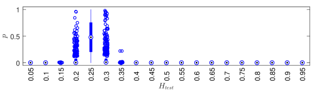
Figure 1: $p$-values obtained from $T=1000$ Monte Carlo simulations from testing $\mathcal{H}_{0}$ for any $H_{test}\in\{0.05,0.1,\ldots,0.95\}.$ The significant level was $\alpha=0.05$ and the $H_{real}=0.25.$

$H_{test}$	0.05	0.1	0.15	0.2	0.25	0.3	0.35	0.4	0.45	0.5
$\mathcal{H}_{0}$	0	0	0	233	924	249	2	0	0	0
$\mathcal{H}_{1}$	1000	1000	1000	767	76	751	998	1000	1000	1000
$H_{test}$		0.55	0.6	0.65	0.7	0.75	0.8	0.85	0.9	0.95
$\mathcal{H}_{0}$		0	0	0	0	0	0	0	0	0
$\mathcal{H}_{1}$		1000	1000	1000	1000	1000	1000	1000	1000	1000

Table 1: Numbers of accepting of $\mathcal{H}_{0}$ or $\mathcal{H}_{1}$ at the significant level $\alpha=0.05$ for the case with $H_{real}=0.25$ obtained from $T=1000$ Monte Carlo simulations.

The next case is a validation of the proposed test for exemplary superdiffusion case with $H_{real}=0.75.$ Analogous simulations produced 19 sets of $p$-values corresponding $H_{test}\in\{0.05,0.1,\ldots,0.95\}.$ The each set contains 1000 $p$-values presented as a boxplot on the Figure 2. The results for $H_{test}<0.65$ are almost all $p<0.05$ and that is the strong statistical evidence to reject incorrect $\mathcal{H}_{0}.$ For cases with $H_{test}=0.7$ and $H_{test}>0.75$ the test works not so good as for previous subdiffusion scenario. It incorrectly accepts $\mathcal{H}_{1}$ more than 80% times for $H_{test}=0.7$ and $H_{test}=0.8$ and around 60% times for $H_{test}>0.8.$ So for those cases the type II error is committed very often and the power of the test is weak. On the other hand in the case when $H_{test}=0.75$ and $\mathcal{H}_{0}$ is true we obtained 63 results with $p<0.05.$ In other words we made a type I error 6.3% of $T=1000$ tests. The detailed numbers of accepting of $\mathcal{H}_{0}$ or $\mathcal{H}_{1}$ for the case with $H_{real}=0.75$ we present in Table 2.

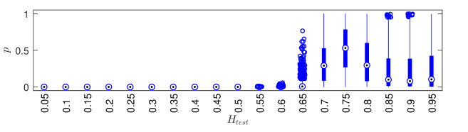
Figure 2: $p$-values obtained from $T=1000$ Monte Carlo simulations from testing $\mathcal{H}_{0}$ for any $H_{test}\in\{0.05,0.1,\ldots,0.95\}.$ The significant level was $\alpha=0.05$ and $H_{real}=0.75.$

$H_{test}$	0.05	0.1	0.15	0.2	0.25	0.3	0.35	0.4	0.45	0.5
$\mathcal{H}_{0}$	0	0	0	0	0	0	0	0	0	0
$\mathcal{H}_{1}$	1000	1000	1000	1000	1000	1000	1000	1000	1000	1000
$H_{test}$		0.55	0.6	0.65	0.7	0.75	0.8	0.85	0.9	0.95
$\mathcal{H}_{0}$		0	1	233	844	937	835	611	568	582
$\mathcal{H}_{1}$		1000	999	767	156	63	165	389	432	420

Table 2: Numbers of accepting of $\mathcal{H}_{0}$ or $\mathcal{H}_{1}$ at the significant level $\alpha=0.05$ for the case with $H_{real}=0.75$ obtained from $T=1000$ Monte Carlo simulations.

5 Conclusion

In this work, we proposed a new statistical test to identify the FBM model in empirical data. This tool is based on the exact probability distribution of the DMA test statistic $\sigma^{2}(n)$, which is very sensitive due to the Hurst index $H.$ The proposed procedure is a new original result in the theory of statistical inference of Gaussian processes.

Conducted Monte Carlo simulations indicate that the constructed test works worse in the case of the superdiffusion when $H>1/2.$ In such a scenario, the type II error is very often committed and the power of the test seems to be weaker than for the subdiffusion. This is due to the fact that for the superdiffusion, the domains of the test statistic $\sigma^{2}(n)$ are close to each other and have joint parts to differing $H$ parameters. This is not the case for subdiffusion where the test works much better. However, it should be strongly emphasized that for both sub and superdiffusion the type I error occurs very rarely and the test correctly accepts the null hypothesis when it is true. In connection with such a test performance and the type II errors, it is possible to modify and optimize the proposed procedure. Namely, a better test performance can be obtained by selecting the argument $n$ of the test statistic $\sigma^{2}(n).$ It is an interesting issue, worth attention and further research.

Another direction of research on the constructed test is its generalized version due to the unknown parameter of the scale parameter $D.$ In this paper, we assumed a standard FBM with $D=1.$ In the general case with the unknown $D,$ the proposed test should be combined with the pre-estimation of the parameter $D$ by other known methods. However, by applying the theory of the ratios of quadratic Gaussian forms [49], it is possible to generalize the described test to the situation of the unknown and non-estimated parameter $D.$ In this case, the probability distribution of the ratios of quadratic forms will not depend on $D$ at all and this parameter will be irrelevant.

The described test procedure can be applied in a sequential manner according to the grid of the values of the parameter $H.$ This will allow to reject the hypotheses with false $H$ values and accept the FBM hypothesis with the true $H.$ Such performance of the proposed test will also be a method for estimating the Hurst exponent as well as a reliable test procedure.

Finally, we want to point out that the statistical test proposed for FBM can be generalized (due to the theory of Gaussian quadratic forms) for each non-degenerated Gaussian process.

6 Appendix

Here we present the Matlab code for the proposed statistical test.

function [h,p,t]=DMAtest(x,n,H,D,alpha,L)
% 
% This function performs the statistical test for FBM (Fractional Brownian
% Motion) with known scale parameter D and unknown suggested Hurst index H.
% The test statistics is a DMA (Detrended Moving Average) statistic
% computed for empirical vector data x. The test is
% proposed by Grzegorz Sikora.
%
% Input:
% x <- vector of empirical data
% n <- argument of DMA statistic
% H <- Hurst index
% D <- known scale parameter of FBM
% alpha <- significant level
% L <- number of Monte Carlo simulations
%
% Output:
% h <- accepted hypothesis: h=0 null hypothesis, h=1 alternative hypothesis
% p <- p-value
% t <- value of DMA statistic for empirical data x
%
% Written by Grzegorz Sikora 13.02.2018, grzegorz.sikora@pwr.edu.pl

% Step 1)
N=length(x);
xmean=sum(x(repmat([1:n]’,1,N-n+1)+repmat(0:N-n,n,1)))/n;
t=sum((x(n:N)-xmean).^2)/(N-n);

%Step 2)
%Covariance matrix of FBM:
R=repmat([1:N]’,1,N);
C=R’;
X=D*(R.^(2*H)+C.^(2*H)-abs(R-C).^(2*H));

%Covariance matrix of process Y(i):
Y1=zeros(N-n+1,N-n+1);
Y2=Y1;
Y3=Y1;
Y=Y1;
for i=1:N-n+1
    for j=1:N-n+1
        Y1(i,j)=(1-1/n)^2*X(i+n-1,j+n-1);
        Y2(i,j)=(1/(n^2)-1/n)*(sum(X(i+n-1,j:j+n-2))+sum(X(i:i+n-2,j+n-1)));
        Y3(i,j)=1/(n^2)*sum(sum(X(i:i+n-2,j:j+n-2)));
    end
end
Y=Y1+Y2+Y3;
lambda=eig(Y)’;

%Step 3)
U_j=chi2rnd(1,N-n+1,L);

%Step 4)
sigma_j=1/(N-n)*lambda*U_j;

%Step 5)
p=2*min(sum(sigma_j>t)/L,sum(sigma_j<t)/L);
if p<alpha
    h=1;
else
    h=0;
end

References

- [1] Aalo, V.A., Piboongungon, T., Efthymoglou, G.P., 2005. Another look at the performance of MRC schemes in Nakagami-m fading channels with arbitrary parameters. IEEE Trans. Commun. 53, 20022005.
- [2] Alessio, E., Carbone, A., Castelli, G., Frappietro, V., 2002. Second-order moving average and scaling of stochastic time series. Eur. J. Phys. B 27 197.
- [3] Ansari, I.S., Yilmaz, F., Alouini, M.S., Kucur, O., 2014. New results on the sum of Gamma random variates with application to the performance of wireless communication systems over Nakagami-m fading channels. Trans. Emerging Tel. Tech. 28 (1), e2912.
- [4] Arianos, S., Carbone, A., 2017. De trending moving average algorithm: A closed-form approximation of the scaling law. Physica A 382, 9-15.
- [5] Bahamonde, N., Torres, S., Tudor, C.A., 2018. ARCH model and fractional Brownian motion. Stat. Probabil. Lett. 134, 70-78.
- [6] Bashan, A., Bartsch, R., Kantelhardt, J.W., Havlin, S., 2008. Comparison of detrending methods for fluctuation analysis. Physica A, 387, 5080-5090.
- [7] Beichelt, F., 2006. Stochastic Processes in Science, Engineering and Finance. C hapman & Hall/CRC.
- [8] Beran, J., 1994. Statistics for long memory processes. Chapman and Hall, London.
- [9] Bondarenko, V.V., 2012. An iterative algorithm of estimating the parameters of the fractal Brownian motion. J. Automat. Inf. Sci. 44 (7), 62-68.
- [10] Borodin, A.N., 2017. Stochastic Processes. Series: Probability and Its Applications, Birkhäuser Basel.
- [11] Bressloff, P.C., 2014. Stochastic Processes in Cell Biology. Series: Interdisciplinary Applied Mathematics 41, Springer International Publishing.
- [12] Breton, J.C., Coeurjolly, J.F., 2012. Confidence intervals for the Hurst parameter of a fractional Brownian motion based on finite sample size. Statistical inference for stochastic processes 15 (1), 1-26.
- [13] Burnecki, K., Kepten, E., Janczura, J., Bronshtein, I., Garini, Y., Weron, A., 2012. Universal Algorithm for Identification of Fractional Brownian Motion. A Case of Telomere Subdiffusion. Biophysical Journal 103, 1839–1847.
- [14] Capasso, V., Bakstein, D., 2015. An Introduction to Continuous-Time Stochastic Processes: Theory, Models, and Applications to Finance, Biology, and Medicine. Series: Modeling and Simulation in Science, Engineering and Technology, Birkhäuser Basel.
- [15] Carbone, A., 2007. Algorithm to estimate the Hurst exponent of high-dimensional fractals. Phys. Rev. E 76, 056703.
- [16] Carbone, A., 2009. Detrending Moving Average algorithm: a brief review. Science and Technology for Humanity (TIC-STH), IEEE Toronto International Conference.
- [17] Carbone, A., Kiyono, K., 2016. Detrending moving average algorithm: Frequency response and scaling performances. Phys. Rev. E 93, 063309.
- [18] Coeurjolly, J.F., 2000. Simulation and identification of the fractional Brownian motion: a bibliographical and comparative study. Journal of Statistical Software 5 (7).
- [19] Coeurjolly, J.F., 2001. Estimating the parameters of a fractional Brownian motion by discrete variations of its sample paths. Statistical Inference for stochastic processes 4 (2), 199-227.
- [20] Coeurjolly, J.F., 2008. Hurst exponent estimation of locally self-similar Gaussian processes using sample quantiles. Ann. Statist. 36 (3), 1404-1434.
- [21] Coeurjolly, J.F., Kortas, H., 2012. Expectiles for subordinated Gaussian processes with applications. Electron. J. Statist. 6, 303-322.
- [22] Cox D.R., Miller, H.D., 2017. The Theory of Stochastic Processes. Chapman & Hall/CRC.
- [23] Davidson, J., Hashimzade, N., 2009 Type I and type II fractional Brownian motions: A reconsideration. Comput. Stat. Data Anal. 53 (6), 2089-2106.
- [24] Davies, R.B., 1980. The distribution of a linear combination of x2 random variables. Applied Statistics 29, 323-333.
- [25] Durrett, R., 2016. Essentials of Stochastic Processes. Springer Texts in Statistics, Springer.
- [26] Efros, A.L., Nesbitt, D.J., 2016. Origin and control of blinking in quantum dots. Nat. Nanotechnol. 11, 661-671.
- [27] El Hajjar, S.T., 2015. A Statistical Study to Provide Estimators of Hurst Parameter for a Fractional Brownian Motion Through Unbalanced Sampling Time. Analysis and Applications 2 (1), 1-8.
- [28] Freund, J.A., Pöschel, T., 2010. Stochastic Processes in Physics, Chemistry and Biology. Series: Lecture Notes in Physics. Springer.
- [29] Fuliński, A., 2017. Fractional Brownian motions: memory, diffusion velocity, and correlation functions. J. Phys. A: Math. Theor. 50, 054002.
- [30] Gu, G.F., Zhou, W.X., 2010. Detrending moving average algorithm for multifractals. Phys. Rev. E 82, 011136.
- [31] Gudowska-Nowak, E., Dybiec, B., 2010. Subordinated diffusion and continuous time random walk asymptotics. Chaos 20, 043129.
- [32] Holcman, D., 2017. Stochastic Processes, Multiscale Modeling, and Numerical Methods for Computational Cellular Biology. Springer International Publishing.
- [33] Jeon, J.H., Metzler, R., 2010. Fractional Brownian motion and motion governed by the fractional Langevin equation in confined geometries. Phys. Rev. E 81, 021103.
- [34] Jiang, Z.Q., Zhou, W.X., 2011. Multifractal detrending moving-average cross-correlation analysis. Phys. Rev. E 84, 016106.
- [35] Kepten, E., Bronshtein, I., Garini, Y., 2011. Ergodicity convergence test suggests telomere motion obeys fractional dynamics Phys. Rev. E 83, 041919.
- [36] Klafter, J., Lim, S.C., Metzler, R., 2012. Fractional Dynamics. Recent Advances, World Scientific, New Jersey.
- [37] Klafter, J., Sokolov, I.M., 2011. First Steps in Random Walks. From Tools to Applications. Oxford University Press, Oxford.
- [38] Kolmogorow, A. , 1940. Wienersche Spiralen und einige andere interessante Kurven in Hilbertschen Raum. C.R. (Doklady) Acad. Sci. URSS (N.S.), 26, 115-118.
- [39] Li, Q., Cao, G., Xu, W., 2018. Relationship research between meteorological disasters and stock markets based on a multifractal detrending moving average algorithm. Int. J. Mod. Phys. B 32, 1750267.
- [40] Li, M., Gençay, R., Xue, Y., 2016. Is it Brownian or fractional Brownian motion? Economics Letters 145, 52-55.
- [41] Lindsey, J.K., 2004. Statistical analysis of stochastic processes in time. Series: Cambridge series in statistical and probabilistic mathematics 14, Cambridge University Press, 2004.
- [42] Lisy, V., Tothova, J., 2018. NMR signals within the generalized Langevin model for fractional Brownian motion. Physica A 494, 200-208.
- [43] Liu, Y., Liu, Y., Wang, K., Jiang, T., Yang, L., 2009. Modified periodogram method for estimating the Hurst exponent of fractional Gaussian noise. Phys. Rev. E 80, 066207.
- [44] Magdziarz, M., Klafter, J., 2010. Detecting origins of subdiffusion. P-variation test for confined systems. Phys. Rev. E 82, 011129.
- [45] Magdziarz, M., Wójcik, J., Ślezak, J., 2013. Estimation and testing of Hurst parameter using p-variation. J. Phys. A: Math. Theor., 46, 325003.
- [46] Mandelbrot, B.B., 1983. The Fractal Geometry of Nature, Freeman, New York.
- [47] Mandelbrot, B.B., Van Ness, J.W., 1968. Fractional Brownian motions, fractional noises and applications. SIAM Rev. 10, 422-437.
- [48] Mathai, A.M., 1982. Storage capacity of a dam with gamma type inputs. Ann. Inst. Stat. Math. 34, 591597.
- [49] Mathai, A.M., Provost, S.B., 1992. Quadratic Forms in Random Variables: Theory and Applications. Marcel Dekker, New York.
- [50] Metzler, R., Klafter, J., 2000. The random walk’s guide to anomalous diffusion: a fractional dynamics approach. Phys. Rep. 339, 1-77.
- [51] Meroz, Y., Sokolov, I.M., 2015. A toolbox for determining subdiffusive mechanisms. Phys. Rep. 573, 1-29.
- [52] Mielniczuk, J., Wojdyłło, P., 2007. Estimation of Hurst exponent revisited. Comput. Stat. Data Anal. 51 (9), 4510-4525.
- [53] Mishura, Y., Shevchenko, G., 2017. Theory and Statistical Applications of Stochastic Processes. Series: Mathematics and Statistics, Wiley-ISTE.
- [54] Moschopoulos, P.G., 1985. The distribution of the sum of independent gamma random variables. Ann. Inst. Stat. Math. 37, 541544.
- [55] Mukeru, S., 2017. Representation of local times of fractional Brownian motion, Stat. Probabil. Lett. 131, 1-12.
- [56] Negro, L., Inampudi, S., 2017. Fractional Transport of Photons in Deterministic Aperiodic Structures. Sci. Rep. 7, 2259.
- [57] Nourdin, I., 2012. Selected aspects of fractional Brownian motion. Series: Bocconi & Springer series 4, Springer.
- [58] Pal, M., Rao, P.M., Manimaran, P., 2014. Multifractal detrended cross-correlation analysis on gold, crude oil and foreign exchange rate time series. Physica A 416, 452-460.
- [59] Palombo, M., Gabrielli, A., De Santis, S., Cametti, C., Ruocco, G., Capuani, S., 2011. Spatio-temporal anomalous diffusion in heterogeneous media by nuclear magnetic resonance. J. Chem. Phys. 135, 034504.
- [60] Paul, W., Baschnagel, J., 2013. Stochastic Processes: From Physics to Finance. Springer International Publishing.
- [61] Ponta, L., Carbone, A., Cincotti, S., 2017. Detrending Moving Average Algorithm: Quantifying Heterogeneity in Financial Data. Computer Software and Applications Conference (COMPSAC), IEEE 41st Annual.
- [62] Rajarshi, M.B., 2013. Statistical Inference for Discrete Time Stochastic Processes. Series: Springer Briefs in Statistics, Springer India.
- [63] Rakotonasy, S.H., Néel, M.C., Joelson, M., 2014. Characterizing anomalous diffusion by studying displacements. Commun. Nonlinear Sci. Numer. Simul. 19, 2284-2293.
- [64] Rao, M.M., 2014. Stochastic Processes - Inference Theory. Series: Springer Monographs in Mathematics, Springer International Publishing.
- [65] Schinazi, R.B., 2014. Classical and Spatial Stochastic Processes: With Applications to Biology. Birkhäuser.
- [66] Schuster, P., 2016. Stochasticity in Processes: Fundamentals and Applications to Chemistry and Biology. Series: Springer Series in Synergetics, Springer International Publishing.
- [67] Scott M., 2012. Applied stochastic processes in science and engineering. U. Waterloo.
- [68] Serinaldi, F., 2010. Use and misuse of some Hurst parameter estimators applied to stationary and non-stationary financial time series. Physica A 389 (14), 2770-2781.
- [69] Shao, Y.H., Gu, G.F., Jiang, Z.Q., Zhou, W.X., 2015. Effects of polynomial trends on detrending moving average analysis. Fractals 23 (3), 1550034.
- [70] Shao, Y.H., Gu, G.F., Jiang, Z.Q., Zhou, W.X., Sornette, D., 2012. Comparing the performance of FA, DFA and DMA using different synthetic long-range correlated time series. Sci. Rep. 2, 835.
- [71] Sikora, G., Burnecki, K., Wyłomańska, A., 2017. Mean-squared-displacement statistical test for fractional Brownian motion. Phys. Rev. E 95, 032110.
- [72] Song, I., Lee, S., 2015. Explicit formulae for product moments of multivariate Gaussian random variables. Stat. Probabil. Lett. 100, 27-34.
- [73] Szymanski, J., Weiss, M., 2009. Elucidating the Origin of Anomalous Diffusion in Crowded Fluids. Phys. Rev. Lett. 103, 038102.
- [74] Taqqu M., Teverovsky V., 1995. Estimators for long-range dependence: an empirical study. Fractals 3 (4), 785-798.
- [75] Van Kampen, N.G., 2007. Stochastic Processes in Physics and Chemistry. Series: North-Holland personal library, Elsevier.
- [76] Vellaisamy P., Upadhye, N.S., 2009. On the sums of compound negative binomial and gamma random variables. J. Appl. Probab. 46, 272-283.
- [77] Wang, W., Chen, Z., 2018. Large deviations for subordinated fractional Brownian motion and applications, J. Math. Anal. Appl. 458 (2), 1678-1692.
- [78] Weiss, M., 2013. Single-particle tracking data reveal anticorrelated fractional Brownian motion in crowded fluids. Phys. Rev. E 88, 010101(R).
- [79] Xi, C., Zhang, S., Xiong, G., Zhao, H., 2016. A comparative study of two-dimensional multifractal detrended fluctuation analysis and two-dimensional multifractal detrended moving average algorithm to estimate the multifractal spectrum. Physica A 454, 34-50.
- [80] Xiong, G., Zhang, S., Zhao, H., 2014. Multifractal spectrum distribution based on detrending moving average. Chaos, Solitons & Fractals 65, 97-110.
- [81] Yerlikaya-Özkurt, F., Vardar-Acar, C., Yolcu-Okur, Y., Weber, G.W., 2014. Estimation of the Hurst parameter for fractional Brownian motion using the CMARS method. Journal of Computational and Applied Mathematics 259, 843-850.
- [82] Zhang, Q., Zhou, Y., Singh, V.P., Chen, Y.D., 2011. Comparison of detrending methods for fluctuation analysis in hydrology. Journal of Hydrology 400 (1–2), 121-132.