Linear model predictive safety certification for learning-based control

Abstract

While it has been repeatedly shown that learning-based controllers can provide superior performance, they often lack of safety guarantees. This paper aims at addressing this problem by introducing a model predictive safety certification (MPSC) scheme for linear systems with additive disturbances. The scheme verifies safety of a proposed learning-based input and modifies it as little as necessary in order to keep the system within a given set of constraints. Safety is thereby related to the existence of a model predictive controller (MPC) providing a feasible trajectory towards a safe target set. A robust MPC formulation accounts for the fact that the model is generally uncertain in the context of learning, which allows for proving constraint satisfaction at all times under the proposed MPSC strategy. The MPSC scheme can be used in order to expand any potentially conservative set of safe states and we provide an iterative technique for enlarging the safe set. Finally, a practical data-based design procedure for MPSC is proposed using scenario optimization.

I Introduction

Learning-based control introduces new ways for controller synthesis based on large-scale databases providing cumulated system knowledge. This allows for previously intense tasks, such as system modeling and controller tuning, to eventually be fully automated. For example, deep reinforcement learning provides prominent results, with applications including control of humanoid robots in complex environments [1] and playing Atari Arcade video-games [2].

Despite the advances in research-driven applications, the results can often not be transferred to industrial systems that are safety-critical, i.e. that must be guaranteed to operate in a given range of physical and safety constraints. This is due to the often complex functioning of learning-based methods rendering their systematic analysis difficult.

By introducing a model predictive safety certification (MPSC) mechanism for any learning-based controller, we aim at bridging this gap for linear systems with additive uncertainties that can, e.g., result from a belief representation of an unknown non-linear system. The proposed MPSC scheme estimates safety of a proposed learning-based input in real-time by searching for a safe back-up trajectory for the next time step in the form of generating a feasible trajectory towards a known safe set. Allowing the MPSC scheme to modify the potentially unsafe learning-based input, if necessary, provides safety for all future times. The result can be seen as a ‘safety filter’, since it only filters proposed inputs that drive the system out of what we call the safe set. The resulting online optimization problem can be efficiently solved in real-time using established model predictive (MPC) solvers. Partially unknown larger-scale systems can therefore be efficiently enhanced with safety certificates during learning.

Contributions: We consider linear systems with additive disturbances, described in Section II, that encode the current, possibly data-driven, belief about a safety-critical system to which a potentially unsafe learning-based controller should be applied. A model predictive safety certification scheme is proposed in Section III, which allows for enhancing any learning-based controller with safety guarantees. The concept of the proposed scheme is comparable to the safety frameworks presented in [3, 4] by providing an implicit safe set together with a safe backup controller that can be applied if the system would leave the safe set using the proposed learning input. A distinctive advantage compared to existing methods is that the MPSC scheme can build on any system behavior that is known to be safe, i.e. a known set of safe system states can be easily incorporated in our scheme such that it will only analyze safety outside of the provided safe set.

The approach relies on scalable offline computations and online optimization of a robust MPC problem at every sampling time, which can be performed using available real-time capable solvers that can deal with large-scale systems (see e.g. [5]). While we relate the required assumptions and design steps to tube-based MPC in Section IV, we present an automated, parametrization free, and data-driven design procedure, that is tailored to the context of learning the system dynamics. The design procedure and MPSC scheme are illustrated in Section V using numerical examples.

Related work: Making the relevant class of safety critical systems accessible to learning-based control methods has gained significant attention in recent years. In addition to the individual construction of safety certificates for specific learning-based control methods subject to different notions of safety, see e.g. the survey [6], a discussion of advances in safe learning-based control subject to state and input constraints can be found in [7]. A promising direction that emerged from recent research focuses on what is called a ‘safety framework’ [3, 7, 4, 8], which consists of a safe set in the state space and a safety controller. While the system state is contained in the safe set, any feasible input (including learning-based controllers) can be applied to the system. However, if such an input would cause the system to leave the safe set, the safety controller interferes. Since this strategy is compatible with any learning-based control algorithm, it serves as a universal safety certification concept. The techniques proposed in [3, 7] are based on a differential game formulation that results in solving a min-max optimal control problem, which can provide the largest possible safe set, but offers very limited scalability. The approach described in [4] uses convex approximation techniques that scale well to larger-scale systems at the cost of a potentially conservative safe set. While these results explicitly consider non-linear systems, we focus on linear model approximations allowing for various improvements. We introduce a new mechanism for generating the safe set and controller using ideas related to tube-based MPC, which enables scalability with respect to the state dimension, while being less conservative than e.g. [4].

There is a methodological similarity to learning-based MPC approaches, as e.g. proposed in [9], or more recently in [10] considering nonlinear Gaussian process models. While such methods are limited to an MPC strategy based on the learned system model, this paper provides a concept that can enhance any learning-based controller with safety guarantees. This allows, e.g., for maximizing black-box reward functions (reward of a sequence of actions is only available through measurements) for complex tasks, see e.g. [11], which would not be possible within an MPC framework, or to focus on exploration in order to collect informative data about the system, as described in Section V.

Notation: The set of symmetric matrices of dimension $n$ is $S^{n}$, the set of positive (semi-) definite matrices is ($S^{n}_{+}$) $S^{n}_{++}$, the set of integers in the interval $[a,b]\subset\mathbb{R}$ is $\mathcal{I}_{[a,b]}$, and the set of integers in the interval $[a,\infty)\subset\mathbb{R}$ is $\mathcal{I}_{\geq a}$. The Minkowski sum of two sets $\mathcal{A}_{1},\mathcal{A}_{2}\subset\mathbb{R}$ is denoted by $\mathcal{A}_{1}\oplus\mathcal{A}_{2}$ and the Pontryagin set difference by $\mathcal{A}_{1}\ominus\mathcal{A}_{2}$. The $i$-th row and $i$-th column of a matrix $A\in\mathbb{R}^{n\times m}$ is denoted by $\mathrm{row}_{i}(A)$ and $\mathrm{col}_{i}(A)$.

II Problem description

We consider dynamical systems, which can be described by linear systems with additive disturbances of the form

$$x(k+1)=Ax(k)+Bu(k)+w(k)$$ (1)

with initial condition $x(0)=x_{0}$ and $w(k)\in\mathcal{W}$ where $\mathcal{W}$ is a compact set. The system is subject to polytopic state constraints $x(k)\in\mathbb{X}\coloneqq\{x\in\mathbb{R}^{n}|A_{x}x\leq b_{x}\}$, $A_{x}\in\mathbb{R}^{n_{x}\times n}$, $b_{x}\in\mathbb{R}^{n_{x}}$ and polytopic input constraints $u(k)\in\mathbb{U}\coloneqq\{u\in\mathbb{R}^{m}|A_{u}u\leq b_{u}\}$, $A_{u}\in\mathbb{R}^{n_{u}\times m}$, $b_{u}\in\mathbb{R}^{n_{u}}$. We assume that the origin is contained in $\mathbb{X}$, $(A,B)$ is stabilizable, and the system state is fully observable. Note that system class (1) allows for modeling nonlinear time-varying systems $x(k+1)=f(k,x(k),u(k))$ if $x(k+1)\in Ax(k)+Bu(k)\oplus\mathcal{W}$ for all $(x,u)\in(\mathbb{X},\mathbb{U})$.

We aim at providing a safety certificate for arbitrary control signals in terms of a safe set and a safe control law. Given the system description (1) and a potentially unsafe learning-based controller $u_{\mathcal{L}}$, we search for a set of states $\mathcal{S}$ for which we know a feasible backup control strategy $u_{\mathcal{B}}$ such that input and state constraints will be fulfilled for all future times. Therefore, $u_{\mathcal{L}}$ can be applied as long as it does not cause the system to leave $\mathcal{S}$ or violate input constraints. Otherwise, a safety controller $u_{\mathcal{S}}$ is allowed to modify the learning input based on the backup controller in order to keep the system safe. Formally this is captured by the following definition of a safe set and controller.

Definition II.1.

A set $\mathcal{S}\subseteq\mathbb{X}$ is called a safe set for system (1) if a safe backup control law $u_{\mathcal{B}}:\mathbb{R}^{n}\times\mathbb{R}^{m}\times\mathcal{I}_{\geq 0}\rightarrow\mathbb{U}$ is available such that for an arbitrary (learning-based) policy $u_{\mathcal{L}}:\mathcal{I}_{\geq 0}\rightarrow\mathbb{R}^{m}$, the application of the safety control law

$$u_{\mathcal{S}}(k)\coloneqq\begin{cases}u_{\mathcal{L}}(k),~{}\text{if}~{}u_{\mathcal{L}}\in\mathbb{U}\land\{Ax+Bu_{\mathcal{L}}\}\oplus\mathcal{W}\subseteq\mathcal{S}\\ u_{\mathcal{B}}(x(k),u_{\mathcal{L}}(k),k),~{}\text{otherwise}\end{cases}$$

guarantees that the system state $x(k)$ is contained in $\mathbb{X}$ for all $k\geq\bar{k}$ if $x(\bar{k})\in\mathcal{S}$.

While this framework is conceptually similar to those in [3, 7, 4, 8], we do not require the safe set $\mathcal{S}$ to be robust controlled invariant as in [4, Definition II.4], [7, Definition 2], [8, Section 2.2] or [3, Section II.A]. The presented approach is thereby capable of enlarging any given safe set, and can be combined with any of the previously proposed methods.

III Model predictive safety certification

Figure 1: Model predictive safe set (blue) based on available data points (red): Belief-based safe optimal trajectory that supports $u_{\mathcal{L}}(k)$, starting nearby $x(t)$ and resulting in the safe terminal set, with uncertainty tubes, that will contain the real system state.

The starting point for the derivation of the proposed safety concept is Definition II.1. The essential requirement is that in the safe set $\mathcal{S}$, we always need to know a feasible backup controller $u_{\mathcal{B}}$, that ensures constraint satisfaction in the face of uncertainty for all future times. The idea for constructing such a controller is based on MPC [12]. Given the current system state, we calculate a safe, finite horizon backup controller towards some conservative target set $\mathcal{S}_{f}$, which is known to be a safe set and therefore provides ‘infinite safety’ after applying the finite-time controller.

The concept is illustrated in Figure 1. Consider a current system state $x(k)$, together with a proposed learning input $u_{\mathcal{L}}(k)$. In order to analyze safety of $u_{\mathcal{L}}(k)$, we test if $u_{\mathcal{L}}(k)$ will lead us to a state $x(k+1)$, for which we can construct a safe backup controller $u_{\mathcal{B}}$ in the form of a feasible input sequence that drives the system to the safe terminal set $\mathcal{S}_{f}$ in a given finite number of steps. If the test is successful, $x(k+1)$ is a safe state and $u_{\mathcal{L}}(k)$ can be applied. At the next time step $k+1$, we repeat the calculations for $x(k+1)$ and $u_{\mathcal{L}}(k+1)$. If it is successful, we can again apply the learning input $u_{\mathcal{L}}(k+1)$, otherwise we can simply use the previously calculated backup controller from time $k$. This strategy yields a safe set that is defined by the feasible set of the corresponding optimization problem for planning a trajectory towards the target set.

As the true system dynamics model is often unknown in the context of learning-based control, we employ mechanisms from tube-based MPC to design a safe backup controller for uncertain system dynamics of the form (1).

III-A Model predictive safety certification scheme

Similar as in tube-based MPC, see e.g. [12], a nominal backup trajectory is computed, such that a stabilizing auxiliary controller is able to track it for the real system within a ‘tube’ towards the safe terminal set. We first define the main components and assumptions of the tube-based MPC controller, in order to then introduce the model predictive safety certification (MPSC) scheme, consisting of the MPSC problem and the proposed safety controller. Define with $z(k)\in\mathbb{R}^{n}$ and $v(k)\in\mathbb{R}^{m}$ the nominal system states and inputs, as well as the nominal dynamics

$$z(k+1)=Az(k)+Bv(k),~{}k\in\mathcal{I}_{\geq 0}$$ (2)

with initial condition $z(0)=z_{0}$. Denote $e(k)\coloneqq x(k)-z(k)$ as the error (deviation) between the system state (1) and the nominal system state (2). The controller is then defined by augmenting the nominal input with an auxiliary feedback on the error, i.e.

$$u(k)=v(k)+K_{\Omega}(x(k)-z(k)),$$ (3)

which keeps the real system state $x(k)$ close to the nominal system state $z(k)$ if $K_{\Omega}\in\mathbb{R}^{m\times n}$ is chosen such that it robustly stabilizes the error $e(k)\coloneqq x(k)-z(k)$ with dynamics

$$e(k+1)=(A+BK_{\Omega})e(k)+w(k)$$ (4)

resulting from application of (3) to the real system.

Assumption III.1.

There exists a linear state feedback matrix $K_{\Omega}\in\mathbb{R}^{m\times n}$ that yields a stable error system (4).

Stability of the autonomous error dynamics (4) implies the existence of a corresponding robust positively invariant set according to the following definition.

Definition III.2.

A set $\Omega\subseteq\mathbb{R}^{n}$ is a robust positively invariant (RPI) set for the error dynamics (4) if

$$e(k_{0})\in\Omega\Rightarrow e(k)\in\Omega\text{ for all }k\in\mathcal{I}_{\geq k_{0}}.$$

In order to guarantee that $(x,u)\in\mathbb{X}\times\mathbb{U}$ under application of (3), the state and input constraints $\mathbb{X}$ and $\mathbb{U}$ are tightened for the nominal system (2), as described e.g. in [12], to $\bar{\mathbb{X}}=\mathbb{X}\ominus\Omega$ and $\bar{\mathbb{U}}=\mathbb{U}\ominus K_{\Omega}\Omega$. There exist various methods in the literature, which can be used in order to calculate a controller and the corresponding RPI set according to Definition III.2, see e.g. [13].

Different from standard tube-based MPC, the model predictive safety certification (MPSC) uses a terminal set that is only required to be itself a safe set according to Definition II.1, which is conceptually similar to the safe terminal set used in [10]. This allows not only for enlarging any potentially conservative initial safe set, but also for recursively improving the safe set, as will be shown in Section IV-B.

Assumption III.3.

There exists a safe set $\mathcal{\mathcal{S}}_{f}\subseteq\mathbb{X}$ and a safe control law $u_{\mathcal{S}_{f}}$ according to Definition II.1 such that $\Omega\subseteq\mathcal{S}_{f}$.

Remark III.4.

Note that a standard terminal set as, e.g. described in [12], also satisfies Assumption III.3. A trivial choice is therefore $\mathcal{\mathcal{S}}_{f}=\Omega$ and $u_{\mathcal{S}_{f}}(k)=K_{\Omega}x(k)$.

Based on these components, the proposed safe backup controller utilizes the following MPSC problem for a given measured state $x$ and proposed learning input $u_{\mathcal{L}}$:

$$\min_{\begin{subarray}{c}{v}_{0},..,{v}_{N-1},\\ {z}_{0},..,{z}_{N},\tilde{u}\end{subarray}}~{} \left\lVert{u_{\mathcal{L}}-\tilde{u}}\right\rVert$$ (5a)

s.t. $${z}_{i+1}=A{z}_{i}+B{v}_{i},~{}\forall i\in\mathcal{I}_{[0,N-1]}$$ (5b)

$$({z}_{i},{v}_{i})\in\bar{\mathbb{X}}\times\bar{\mathbb{U}},~{}\forall i\in\mathcal{I}_{[0,N-1]}$$ (5c)

$${z}_{N}\in\mathcal{\mathcal{S}}_{f}\ominus\Omega$$ (5d)

$$x-z_{0}\in\Omega$$ (5e)

$$\tilde{u}={v}_{0}+K_{\Omega}(x-{z}_{0})$$ (5f)

where we denote the planning horizon by $N\in\mathcal{I}_{\geq 1}$ and the predicted nominal system states and inputs by ${z}_{i}$ and ${v}_{i}$. Let the feasible set of (5) be denoted by

$$\mathcal{X}_{N}\coloneqq\{x\in\mathbb{R}^{n}|\eqref{eq:MPSC_opt_nominal_dynamics}-\eqref{eq:MPSC_aux_vars_constraints}\}\subseteq\mathbb{X}.$$ (6)

Problem (5) introduces the auxiliary variable $\tilde{u}$, which includes the auxiliary feedback (5f), ensuring safety of the control input $\tilde{u}$, as we will show in the proof of Theorem III.5. The cost (5a) is chosen such that if possible, $\tilde{u}$ is equal to $u_{\mathcal{L}}$, in which case safety of $u_{\mathcal{L}}$ is certified. The controller resulting from (5) in a receding horizon fashion is given by

$$\kappa(x)=\tilde{u}^{*}(x)$$ (7)

where ${v}_{0}^{*}(x),..,{v}_{N-1}^{*}(x)$, ${z}_{0}^{*}(x),..,{z}_{N}^{*}(x)$, and $\tilde{u}^{*}(x)$ is the optimal solution of (5) at state $x$.

It is important to note that (5) may not be recursively feasible for general safe sets $\mathcal{S}_{f}$. This is due to the fact that the terminal safe set $\mathcal{S}_{f}$ is itself not necessarily invariant or a subset of the feasible set.

To this end, we propose Algorithm 1, which implements a safety controller based on (5). If $x(k)\in\mathcal{X}_{N}$ we can always directly apply $\tilde{u}$ (Algorithm 1, line 4). If at a subsequent time $x(k+1)\notin\mathcal{X}_{N}$, then we know via (5) a finite-time safe backup controller towards $\mathcal{S}_{f}$ using (3), from the trajectory computed to certify $x(k)$ (Algorithm 1, line 9), compare also with Figure 1. By Assumption III.3 we can extend this finite-time backup controller after $N$-steps with $u_{\mathcal{S}_{f}}$ (Algorithm 1, line 11) in order to obtain a safe backup controller for $x(k+i),i\geq 0$, which will satisfy constraints at all times in the future. In the case that $\mathcal{S}_{f}\setminus\mathcal{X}_{N}\neq\emptyset$, (5) can be initially infeasible for $x=x(0)\in\mathcal{S}_{f}$. This case can be easily treated by directly applying $u_{\mathcal{S}_{f}}$ (Algorithm 1, line 1 and line 11) which ensures safety for all future times. Formalization of the above yields our main result.

Algorithm 1 Model predictive safety certification scheme

1:$k_{\text{inf}}:=N-1$

2:for $k=0,1,2,...$ do

3:    if (5) feasible then

4:         Apply $u(k):=\kappa(x(k))$ to (1)

5:         $k_{\text{inf}}:=0$

6:    else

7:         $k_{\text{inf}}:=k_{\text{inf}}+1$

8:         if $k_{\text{inf}}\leq N-1$ then

9:             Apply $u(k):={v}^{*}_{k_{\text{inf}}}+K_{\Omega}(x(k)-{z}^{*}_{k_{\text{inf}}})$ to (1)

10:         else

11:             Apply $u(k):=u_{\mathcal{S}_{f}}(k)$ to (1)

12:         end if

13:    end if

14:end for

Theorem III.5.

If Assumptions III.1 and III.3 hold, then the control law resulting from Algorithm 1 is a safe backup controller and $\mathcal{X}_{N}\cup\mathcal{S}_{f}$ the corresponding safe set according to Definition II.1.

Proof.

If $x(0)\in\mathcal{S}_{f}\setminus\mathcal{X}_{N}$, the terminal safety controller $u_{\mathcal{S}_{f}}$ is applied since $k_{\text{inf}}$ is initialized to $N-1$ in (Algorithm 1, line 1), which keeps the system safe for all times. We show that $\mathcal{X}_{N}$ is a safe set by first investigating the case that (5) is feasible for all $k\in\mathcal{I}_{\geq 0}$ and extending the analysis to cases in which (5) is infeasible for arbitrarily many time steps.

Let $x(0)\in\mathcal{X}_{N}$ and let (5) be feasible for all $k\in\mathcal{I}_{\geq 0}$ (Algorithm 1, line 4), i.e. $x(k)\in\mathcal{X}_{N}$. Condition (5e) implies by Assumption III.1 that $e(k+1)\in\Omega$ and therefore that $x(k+1)\in{z}_{1}\oplus\Omega$, which implies by the tightened constraints on the nominal state (5c) that $x(k+1)\in\mathbb{X}$. Therefore $\mathcal{X}_{N}$ is a safe set under the safe backup controller $\kappa(x)$ in (7).

Now, consider an arbitrary time $\bar{k}$ for which $\eqref{eq:MPSC_opt}$ was feasible for the last time, i.e. $x(k)\notin\mathcal{X}_{N}$ for all $k=\bar{k}+k_{\text{inf}}$ with $k_{\text{inf}}\in\mathcal{I}_{[1,N-1]}$. Because of (5e) and (5f) we have that $e(\bar{k}+1)\in\Omega$ and therefore Assumption III.3 together with (5d) allows for explicitly stating a safe backup control law based on $x=x(\bar{k})\in\mathcal{X}_{N}$ that keeps the system in the constraints for all future times:

$$u_{\mathcal{B}}(x(i),x,i)=$$

$$\quad\begin{cases}{v}_{i-\bar{k}}^{*}(x)+K_{\Omega}(x(i-\bar{k})-{z}_{i-\bar{k}}^{*}(x))),i\in\mathcal{I}_{[\bar{k}+1,\bar{k}+N-1]}\\ u_{\mathcal{S}_{f}}(i),i\in\mathcal{I}_{\geq\bar{k}+N}.\end{cases}$$

Since (5) was feasible for $x(\bar{k})$, the corresponding ${v}^{*}_{1},..,{v}^{*}_{N-1}$, ${z}^{*}_{1},..,{z}^{*}_{N}$ exist. Therefore in case of $x(k)\notin\mathcal{X}_{N}$, Algorithm 1, line 9 and $k_{\text{inf}}\in\mathcal{I}_{[1,N-1]}$, it follows from $e(\bar{k}+1)\in\Omega$ by Assumption III.1 that $x(\bar{k}+k_{\text{inf}})\in{z}^{*}_{k_{\text{inf}}}\oplus\Omega$ for all $k_{\text{inf}}\in\mathcal{I}_{[1,N-1]}$.

The last remaining case $k_{\text{inf}}\geq N$ follows from the observation, that $x(\bar{k}+N)\in\mathcal{S}_{f}$ by (5d) for which we know the safe control law $u_{\mathcal{S}_{f}}$ for all future times by Assumption III.3. Once a feasible solution is found again, the counter $k_{\text{inf}}$ is set to zero. Consequently we investigated all possible cases in Algorithm 1 and proved that it will always provide a safe control input if $x(0)\in\mathcal{X}_{N}\cup\mathcal{S}_{f}$, showing the result. ∎

III-B A recursively feasible MPSC scheme

By modifying Assumption III.3 and requiring the terminal safe set to be invariant for the nominal system, which is the standard assumption in tube-based MPC, we obtain recursive feasibility of (5) and can thus directly apply the time-invariant control law (7) to system (1) without the need of Algorithm 1. In other words, (7) directly becomes the safety controller according to Definition II.1.

Assumption III.6.

There exists a set $\mathcal{X}_{f}\subseteq\bar{\mathbb{X}}$ and corresponding control law $\sigma_{f}:\mathcal{X}_{f}\rightarrow\bar{\mathbb{U}}$ such that for all $z\in\mathcal{X}_{f}$, $\Rightarrow Az+B\sigma_{f}(z)\in\mathcal{X}_{f}$.

Theorem III.7.

Let $\mathcal{S}_{f}=\mathcal{X}_{f}\oplus\Omega$. If Assumptions III.1, and III.6 hold, then (7) is a safe backup control law and $\mathcal{X}_{N}$ the corresponding safe set according to Definition II.1. In addition, $\mathcal{X}_{N}$ is a robust positively invariant set.

Proof.

We begin with showing recursive feasibility under (7). Let (5) be feasible at time $k$. It follows that $x(k+1)\in{z}^{*}_{1}\oplus\Omega$ because of (5e) and (5f). From here, recursive feasibility follows as in standard tube-based MPC by induction, see e.g. [12]. Along the lines of the proof of Theorem III.5, recursive feasibility implies that $\mathcal{X}_{N}$ is a safe set. ∎

IV Design of $\mathcal{S}_{f}$ and $\Omega$ from data

The proposed MPSC scheme is based on two main design components, the robust positively invariant set $\Omega$, which determines the tube, and the terminal safe set $\mathcal{S}_{f}$.

While $\mathcal{S}_{f}$ can be chosen more generally according to Assumption III.3, we note from Theorem III.7 that we can in principle also use the same design methods proposed for linear tube-based MPC. The computation of the robust invariant set $\Omega$ and the nominal terminal set $\mathcal{X}_{f}$ have been widely studied in the literature, see e.g. [12, 14] and references therein.

This section presents a different option for the approximation of a tube and safe terminal set that is tailored to the learning context and aims at a minimal amount of tuning ‘by hand’. We propose to infer a robust control invariant set $\Omega$ either directly from data or from a probabilistic model via scenario-based optimization. Secondly, starting from any terminal safe set, e.g. the trivial choice $\{0\}\oplus\Omega$, we show how to enlarge this terminal set iteratively by utilizing feasible solutions of (5) over time.

IV-A Scenario based calculation of $\Omega$ from data

Let $\{\tilde{w}_{i}\}_{i=1}^{N_{s}}$ be a set of so-called ‘scenarios’, either sampled from a probabilistic belief about the system dynamics (1) or collected from measurements. We restrict ourselves to ellipsoidal robust positively invariant sets $\Omega=\{x|x^{\top}Px\leq 1\}$ with $P\in S^{n}_{++}$, in order to enable scalability of the resulting design optimization problems to larger scale systems. The corresponding robust scenario-based design problem for computation of the set $\Omega$ is given by

$$\min_{P\in S^{n}_{++},\tau>0}~{}-\log\det(P)$$ (8a)

$$\text{s.t.}~{}\forall i\in\mathcal{I}_{[1,N_{s}]}:$$

$$~{}\begin{pmatrix}A_{cl}^{\top}PA_{cl}-\tau P&A_{cl}^{\top}P\tilde{w}_{i}\\ \tilde{w}_{i}^{\top}PA_{cl}&\tilde{w}_{i}^{\top}P\tilde{w}_{i}+\tau-1\end{pmatrix}\preceq 0$$ (8b)

where $A_{cl}\coloneqq A+BK_{\Omega}$. Problem (8) defines a robust positively invariant set for the error system (4), if the condition is enforced for all $\tilde{w}_{i}\in\mathcal{W}$, see e.g. [14]. The objective (8a) is chosen such that a possibly small RPI set is obtained, which increases by definition of $\bar{\mathbb{X}}$ and $\bar{\mathbb{U}}$ the size of the feasible region of (5), and therefore the size of the safe set. A stabilizing linear state feedback matrix $K_{\Omega}$ according to Assumption III.1 needs to be chosen beforehand, e.g. using LQR or $\mathcal{H}_{\infty}$ controller design methods.

Proposition IV.1.

Consider system (4) and let $n_{s}\coloneqq(n^{2}+n)/2+1$. If (8) attains a solution, then with probability at least $1-\sum_{i=0}^{n_{s}-1}\begin{pmatrix}N_{s}\\ i\end{pmatrix}\epsilon^{i}(1-\epsilon)^{N_{s}-i}$, the solution is $\epsilon$-level robustly feasible for the corresponding robust problem imposing (8b) for all $\tilde{w}_{i}\in\mathcal{W}$, i.e., the probability that there exists a $\tilde{w}_{i}\in\mathcal{W}$ for which (8b) is violated is less or equal to $\epsilon$.

Proof.

The result follows directly from [15, Theorem 1] similar to the application demonstrated in [16]. ∎

IV-B Iterative enlargement of the terminal safe set $\mathcal{S}_{f}$

In this section we show how to enlarge the terminal safe set $\mathcal{S}_{f}$ based on previously calculated solutions of (5), which is conceptually similar to the data-based terminal set proposed in [17]. Note, that a larger terminal set $\mathcal{S}_{f}$ according to Assumption III.3 or Assumption III.6 typically also leads to a larger feasible set $\mathcal{X}_{N}$, and therefore to a larger overall safe set $\mathcal{S}$ according to Theorems III.5 and III.7.

The main idea is to define a safe set based on successfully solved instances of (5) for measured system states

$$\bm{x}^{*}_{\mathcal{M}(k)}\coloneqq\left\{x(i),i\in\mathcal{M}(k)\right\}$$ (9)

where $\mathcal{M}(k)\coloneqq\{i\in\mathcal{I}_{[0,k]}|x(i)\in\mathcal{X}_{N}\}$ is an index set representing time instances for which the system state $x(i)$ was feasible in terms of (5) during application of Algorithm 1 up to time $k$.

Theorem IV.2.

If Assumptions III.1 and III.3 are satisfied, and (5) is convex, then the set

$$\mathcal{S}_{f}^{\mathcal{M}(k)}\coloneqq\mathrm{co}(\bm{x}^{*}_{\mathcal{M}(k)})\cup\mathcal{S}_{f}$$ (10)

is again a safe set according to Definition II.1 with a safe backup controller given by Algorithm 1.

Proof.

If (5) is convex, then the feasible set is a convex set, see e.g. [18] and therefore $\mathrm{co}(\bm{x}^{*}_{\mathcal{M}(k)})\subseteq\mathcal{X}_{N}$. As a consequence, we can solve (5) for all $x\in\mathrm{co}(\bm{x}^{*}_{\mathcal{M}(k)})$ which in turn provides the result by the proof of Theorem III.5 (by replacing $\mathcal{X}_{N}$ with $\mathrm{co}(\bm{x}^{*}_{\mathcal{M}(k)})$) and the fact that the union of two safe sets is again a safe set. ∎

If $\mathcal{S}_{f}\subseteq\mathrm{co}(\bm{x}^{*}_{\mathcal{M}(k)})$, convexity of the new terminal set (10) is ensured and we can iteratively enlarge the initial terminal set $\mathcal{S}_{f}$.

Remark IV.3.

A practical design procedure in order to determine $\Omega$ and $\mathcal{S}_{f}$ is as follows. Compute $\Omega$ based on measurements as described in Section IV-A and initialize $\mathcal{S}_{f}=\{\Omega\}$. Then, during closed-loop operation of Algorithm 1 enlarge $\mathcal{S}_{f}$ according to (10).

In order to provide a similar result with respect to Theorem III.7 consider the set $\bm{z}^{*}_{\mathcal{M}(k)}=\{{z}^{*}_{1}(x(i)),..,{z}^{*}_{N}(x(i)),i\in\mathcal{M}(k)\}$ with $\mathcal{M}(k)$ as defined above.

Corollary IV.4.

If Assumptions III.1 and III.6 are satisfied, $\mathcal{S}_{f}=\mathcal{X}_{f}\oplus\Omega$, and (5) is convex, then the set

$$\mathcal{X}_{f}^{\mathcal{M}(k)}\coloneqq\mathrm{co}(\bm{z}^{*}_{\mathcal{M}(k)})\cup\mathcal{X}_{f}$$ (11)

satisfies Assumption III.6 and $\mathcal{X}_{f}^{\mathcal{M}(k)}\oplus\Omega$ is a safe set according to Definition II.1 with safe backup controller (7).

Proof.

Follows similarly to the proof of Theorem IV.2. ∎

Using Theorem III.7, we obtain a practical procedure similar to Remark IV.3 by initializing $\mathcal{X}_{f}=\{0\}$ and choosing $\mathcal{X}_{f}^{\mathcal{M}(k)}\oplus\Omega$ as iterative terminal safe set.

Remark IV.5.

Theorem IV.2 also provides an explicit approximation of the safe set given by (10), which is generally only implicitly defined. Such a representation can be used to ‘inform’ the learning-based controller about the safety boundary, e.g. in the form of a feature using a barrier function, in order to avoid chattering behavior, as proposed in [3].

V Application to numerical examples

We consider the problem of safely acquiring information about the partially unknown system dynamics of a discretized mass-spring-damper system, which is given by $x(k+1)=\begin{pmatrix}1&0.1\\ -0.3&0.8\end{pmatrix}x(k)+\begin{pmatrix}0\\ 0.1\end{pmatrix}u(k)$ with $|u(k)|\leq 2.5$, $|x_{1}(k)|\leq 1$, and $x_{2}(k)\in[-0.4,1]$. Assume that an approximate model is given by $x(k+1)=\begin{pmatrix}1&0.1\\ -0.23&0.78\end{pmatrix}x(k)+\begin{pmatrix}0\\ 0.1\end{pmatrix}u(k)+w(k)$ with mass, spring, and damper parameters, which have a 20% error with respect to the true parameters. We use the results from Section IV in order to calculate $\Omega$ without deriving a suitable representation (1), i.e. a suitable $\mathcal{W}$, first. Using the approximate model and LQR design, we choose $K_{\Omega}=(-4.12~{}~{}-5.32)$. Based on $N_{s}=600$ uniformly sampled measurements $\{x_{i},u_{i},y_{i}\}_{i=1}^{N_{s}}$ from the real (but unknown) system, we generate the robust scenario design problem (8) with scenarios $\tilde{w}_{i}=y_{i}-\begin{pmatrix}1&0.1\\ -0.23&0.78\end{pmatrix}x_{i}-\begin{pmatrix}0\\ 0.1\end{pmatrix}u_{i}$. Solving (8) yields that $\Omega=\{x|x^{\top}Px\leq 1\}$ with $P=\begin{pmatrix}53.95&11.47\\ 11.47&14.55\end{pmatrix}$ fulfills (8b) for all possible $\tilde{w}_{i}\in\mathcal{W}$ with probability $0.97$ according to Proposition IV.1. For the MPSC scheme, we use a horizon $N=20$ and the terminal safe set $\mathcal{S}_{f}=\Omega$ as described in Remark IV.3.

As learning signal we use $u_{\mathcal{L}}(k)=2\sin(0.01\pi k)+0.5\sin(0.12\pi k)$ with the goal of generating informative measurements according to [19].

A closed-loop simulation with initial condition $x(0)=(-0.7,1)^{\top}$ under application of Algorithm 1 is illustrated in Figure 2 with the corresponding safe set. As desired, the safety controller modifies the proposed input signal $u_{\mathcal{L}}$ only as the system state approaches a neighborhood of the safe set boundary where the next state would leave the safe set (indicated in red color). The pure learning-based trajectory (dotted line, in Figure 2), in contrast, would have violated state constraints already in the first time steps.

Using a similiar configuration with planning horizon $N=10$, we now iteratively enlarge the safe set based on previously calculated nominal state trajectories at each time step by following Corollary IV.4. Samples of the nominal and overall terminal set at different time steps are shown in Figure 3. After $k=115$ time steps, a significant portion of the state space is already covered by the safe terminal set.

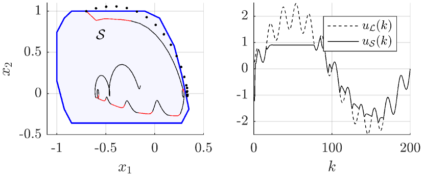
Figure 2: Left: Closed loop simulation under Algorithm 1, starting from $x(0)=[-0.7,1]$. Red color indicates states, for which $\left\lVert{\tilde{u}-u_{\mathcal{L}}}\right\rVert>0$. The dotted line shows the first $20$ time steps of the closed-loop trajectory, resulting from application of $u_{\mathcal{L}}$ without the MPSC scheme. Right: Learning-based control input sequence and applied controller sequence of MPSC scheme.

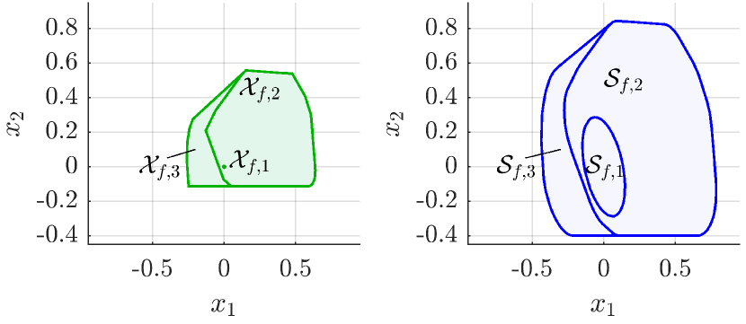
Figure 3: Left: Iterative enlargement of the nominal terminal set (11), which is shown at times $k_{1}=0,k_{2}=100,k_{3}=115$. Right: Resulting safe terminal set $\mathcal{S}_{f}=\mathcal{X}_{f}^{\mathcal{M}(k)}\oplus\Omega$ corresponding to the nominal terminal sets at times $k_{1}=0,k_{2}=100,k_{3}=115$.

VI Conclusion

The paper has addressed the problem of safe learning-based control by means of a model predictive safety certification scheme. The proposed scheme allows for enhancing any potentially unsafe learning-based control strategy with safety guarantees and can be combined with any known safe set. By relying on robust MPC methods, the presented concept is amenable for application to large-scale systems with similar offline computational complexity as e.g. ellipsoidal safe set approximations. Using a parameter-free scenario-based design procedure, it was illustrated how the design steps can be performed based on available data and how to reduce conservatism of the MPSC scheme over time by making use of generated closed-loop data.

References

- [1] J. Merel, Y. Tassa, S. Srinivasan, J. Lemmon, Z. Wang, G. Wayne, and N. Heess, “Learning human behaviors from motion capture by adversarial imitation,” arXiv preprint arXiv:1707.02201, 2017.
- [2] V. Mnih, K. Kavukcuoglu, D. Silver, A. A. Rusu, J. Veness, M. G. Bellemare, A. Graves, M. Riedmiller, A. K. Fidjeland, G. Ostrovski et al., “Human-level control through deep reinforcement learning,” Nature, vol. 518, no. 7540, p. 529, 2015.
- [3] A. K. Akametalu, J. F. Fisac, J. H. Gillula, S. Kaynama, M. N. Zeilinger, and C. J. Tomlin, “Reachability-based safe learning with gaussian processes,” in 53rd IEEE Conference on Decision and Control, Dec 2014, pp. 1424–1431.
- [4] K. P. Wabersich and M. N. Zeilinger, “Scalable synthesis of safety certificates from data with application to learning-based control,” arXiv preprint arXiv:1711.11417, 2017.
- [5] A. Domahidi, A. U. Zgraggen, M. N. Zeilinger, M. Morari, and C. N. Jones, “Efficient interior point methods for multistage problems arising in receding horizon control,” in 51st IEEE Conference on Decision and Control (CDC), Dec 2012, pp. 668–674.
- [6] J. García and F. Fernández, “A comprehensive survey on safe reinforcement learning,” Journal of Machine Learning Research, vol. 16, pp. 1437–1480, 2015.
- [7] J. F. Fisac, A. K. Akametalu, M. N. Zeilinger, S. Kaynama, J. Gillula, and C. J. Tomlin, “A general safety framework for learning-based control in uncertain robotic systems,” arXiv preprint arXiv:1705.01292, 2017.
- [8] R. B. Larsen, A. Carron, and M. N. Zeilinger, “Safe learning for distributed systems with bounded uncertainties,” 20th IFAC World Congress, vol. 50, no. 1, pp. 2536 – 2542, 2017.
- [9] A. Aswani, H. Gonzalez, S. S. Sastry, and C. Tomlin, “Provably safe and robust learning-based model predictive control,” Automatica, vol. 49, no. 5, pp. 1216–1226, 2013.
- [10] T. Koller, F. Berkenkamp, M. Turchetta, and A. Krause, “Learning-based model predictive control for safe exploration and reinforcement learning,” arXiv preprint arXiv:1803.08287, 2018.
- [11] H. Mania, A. Guy, and B. Recht, “Simple random search provides a competitive approach to reinforcement learning,” arXiv preprint arXiv:1803.07055, 2018.
- [12] J. B. Rawlings and D. Q. Mayne, Model predictive control: Theory and design. Nob Hill Pub., 2009.
- [13] S. V. Rakovic, E. C. Kerrigan, K. I. Kouramas, and D. Q. Mayne, “Invariant approximations of the minimal robust positively invariant set,” vol. 50, no. 3. IEEE, 2005, pp. 406–410.
- [14] F. Blanchini, “Set invariance in control,” Automatica, vol. 35, no. 11, pp. 1747 – 1767, 1999.
- [15] M. C. Campi and S. Garatti, “The exact feasibility of randomized solutions of uncertain convex programs,” SIAM Journal on Optimization, vol. 19, no. 3, pp. 1211–1230, 2008.
- [16] G. C. Calafiore and M. C. Campi, “The scenario approach to robust control design,” IEEE Transactions on Automatic Control, vol. 51, no. 5, pp. 742–753, 2006.
- [17] U. Rosolia and F. Borrelli, “Learning model predictive control for iterative tasks: a computationally efficient approach for linear system,” IFAC-PapersOnLine, vol. 50, no. 1, pp. 3142–3147, 2017.
- [18] S. Boyd and L. Vandenberghe, Convex optimization. Cambridge university press, 2004.
- [19] L. Ljung, “System identification,” in Signal analysis and prediction. Springer, 1998, pp. 163–173.