Lattice $\phi^{4}$ Field Theory on Riemann Manifolds: Numerical Tests for the 2-d Ising CFT on ${\mathbb{S}}^{2}$

Abstract

We present a method for defining a lattice realization of the $\phi^{4}$ quantum field theory on a simplicial complex in order to enable numerical computation on a general Riemann manifold. The procedure begins with adopting methods from traditional Regge Calculus (RC) and finite element methods (FEM) plus the addition of ultraviolet counter terms required to reach the renormalized field theory in the continuum limit. The construction is tested numerically for the two-dimensional $\phi^{4}$ scalar field theory on the Riemann two-sphere, ${\mathbb{S}}^{2}$, in comparison with the exact solutions to the two-dimensional Ising conformal field theory (CFT). Numerical results for the Binder cumulants (up to 12th order) and the two- and four-point correlation functions are in agreement with the exact $c=1/2$ CFT solutions.

1 Introduction

Lattice Field Theory (LFT) has proven to be a powerful non-perturbative approach to quantum field theory [1]. However the lattice regulator has generally been restricted to flat Euclidean space, $\mathbb{R}^{d}$, discretized on hypercubic lattices with a uniform ultraviolet (UV) cut-off $\Lambda_{UV}=\pi/a$ in terms of the lattice spacing $a$. Here we propose a new approach to enable non-perturbative studies for a range of problems on curved Riemann manifolds. There are many applications that benefit from this. In the study of Conformal Field Theory (CFT), it is useful to make a Weyl transform from flat Euclidean space ${\mathbb{R}}^{d}$ to a compact spherical manifold $\mathbb{S}^{d}$, or in Radial Quantization [2], a Weyl transformation to the cylindrical boundary, $\mathbb{R}\times\mathbb{S}^{d-1}$, of $AdS^{d+1}$. Other applications that could benefit from extending LFT to curved manifolds include two-dimensional condensed matter systems such as graphene sheets [3], four-dimensional gauge theories for beyond the standard model (BSM) strong dynamics [4, 5], and perhaps even quantum effects in a space-time near massive systems such as black holes.

Before attempting a non-perturbative lattice construction, one should ask if a particular renormalizable field theory in flat space is even perturbatively renormalizable on a general smooth Riemann manifold. Fortunately, this question was addressed with an avalanche of important research [6, 7, 8, 9] in the 70s and 80s. A rough summary is that any UV complete field theory in flat space is also perturbatively renormalizable on any smooth Riemann manifold with diffeomorphism invariant counter terms corresponding to those in flat space [9]. Taking this as given, in spite of our limited focus on $\phi^{4}$ theory, we hope this paper is the beginning of a more general non-perturbation lattice formulation for these UV complete theories on any smooth Euclidean Riemann manifolds.

The basic challenge in constructing a lattice on a sphere—or indeed on any non-trivial Riemann manifold—is the lack of an infinite sequence of finer lattices with uniformly decreasing lattice spacing [2, 10, 11]. For example, unlike the hypercubic lattice with toroidal boundary condition, the largest discrete subgroup of the isometries of a sphere is the icosahedron in 2d and the hexacosichoron, or 600 cell, in 3d. This greatly complicates constructing a suitable bare lattice Lagrangian that smoothly approaches the continuum limit of the renormalizable quantum field theory when the UV cut-off is removed. Here we propose a new formulation of LFT on a sequence of simplicial lattices converging to a general smooth Riemann manifold. Our strategy is to represent the geometry of the discrete simplicial manifold using Regge Calculus [12] (RC) and the matter fields using the Finite Element Method (FEM) [13] and Discrete Exterior Calculus (DEC) [14, 15, 16, 17]. Together these methods define a lattice Lagrangian which we conjecture is convergent in the classical (or tree) approximation. However, the convergence fails at the quantum level due to ultraviolet divergences in the continuum limit. To remove this quantum obstruction, we compute counter terms that cancel the ultraviolet defect order by order in perturbation theory. We will refer to the resultant lattice construction as the Quantum Finite Element (QFE) method and give a first numerical test in 2d on ${\mathbb{S}}^{2}$ at the Wilson-Fisher CFT fixed point.

While our current development of a QFE Lagrangian and numerical tests are carried out for the simple case of a 2-d scalar $\phi^{4}$ theory projected on the Riemann sphere we attempt a more general framework. Since the map to the Riemann sphere, ${\mathbb{R}}^{2}\rightarrow{\mathbb{S}}^{2}$, is a Weyl transform, the CFT is guaranteed [18] to be exactly equivalent to the $c$ =1/2 Ising CFT in flat space and therefore presents a convenient and rigorous test of convergence to the continuum theory. More general examples can and will be pursued mapping conformal field theories in flat Euclidean space $\mathbb{R}^{d+1}$ either to $\mathbb{R}\times\mathbb{S}^{d}$, appropriate for radial quantization,

$$ds^{2}_{flat}=\sum^{d+1}_{\mu=1}dx^{\mu}dx^{\mu}=e^{2t}(dt^{2}+d\Omega^{2}_{d})\xrightarrow{Weyl}(dt^{2}+d\Omega^{2}_{d})\;,$$ (1.1)

with $t=\log(r)$ or to the sphere, ${\mathbb{S}}^{d}$,

$$ds^{2}_{flat}=\sum^{d}_{\mu=1}dx^{\mu}dx^{\mu}=e^{\sigma(x)}d\Omega^{2}_{d}\xrightarrow{Weyl}d\Omega^{2}_{d}\;.$$ (1.2)

Current tests of the QFE method for the 3-d Ising model in radial quantization, ${\mathbb{R}}^{3}\rightarrow{\mathbb{R}}\times{\mathbb{S}}^{2}$, are underway, so we take the opportunity here to give a brief introduction to both geometries. By considering the sphere ${\mathbb{S}}^{d}$ as a dimensional reduction of the cylinder ${\mathbb{R}}\times{\mathbb{S}}^{d}$ by taking the length of the cylinder to zero, both cases are conveniently presented together in Appendix A.

The organization of the article is as follows. In Sec. 2 we review the basic Regge Calculus/Finite Element Method framework as a discrete form of the exterior calculus and show its failure for a quantum field theory beyond the classical limit due to UV divergences. The reader is referred to the literature [13, 14, 15, 16] for more details and to Ref. [19] for the extension to Dirac fermions. In Sec. 3 we address the central issue of counter terms in the interacting $\phi^{4}$ theory required to restore the isometries on ${\mathbb{S}}^{2}$ in the continuum limit. Sec. 4 compares our Monte Carlo simulation for fourth and sixth order Binder cumulants with the exactly solvable $c=1/2$ CFT. In Sec. 5 we extend this analysis to the two-point and four-point correlation functions. We fit the operator product expansion (OPE) as a test case of how to extract the central charge, OPE couplings, and operator dimensions.

2 Classical Limit for Simplicial Lattice Field Theory

The scalar $\phi^{4}$ theory provides the simplest example. On a smooth Riemann manifold, $(\mathcal{M},g)$, the action,

$$S=\int_{\mathcal{M}}d^{d}x\sqrt{g}\left[\tfrac{1}{2}g^{\mu\nu}\partial_{\mu}\phi(x)\partial_{\nu}\phi(x)+\tfrac{1}{2}(m^{2}+\widetilde{\xi}_{0}Ric)\phi^{2}(x)+\lambda\phi^{4}(x)+h\phi(x)\right]\;,$$ (2.1)

is manifestly invariant under diffeomorphisms: $x^{\prime}=f(x)\equiv x^{\prime}(x)$. We include the coupling to the scalar Ricci curvature ($\widetilde{\xi}_{0}Ric$), where $\widetilde{\xi}_{0}=(d-2)/(4(d-1))$ and an external constant (scalar) field $h$. $Ric=(d-1)(d-2)/R^{2}$ on the sphere ${\mathbb{S}}^{d}$ of radius $R$. The field, $\phi(x)$, is an absolute scalar or in the language of differential calculus a 0-form with a fixed value at each point $P$ in the manifold, independent of co-ordinate system: $\phi^{\prime}(x^{\prime})=\phi(x(x^{\prime}))$ for $x^{\prime}=f(x)$ . For future reference to the discussion in Sec. 2.2 on the discrete exterior calculus, we identify $\mbox{vol}_{d}=\sqrt{g}\;d^{d}x=\sqrt{g}dx^{1}\wedge\cdots\wedge dx^{d}$, as the volume d-form.

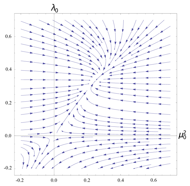
Figure 2.1: The phase plane of $\phi^{4}$ for $d<4$, depicting the renormalization flow from the repulsive weak coupling ultraviolet (UV) fixed point at $(\mu^{2}_{0},\lambda_{0})=(0,0)$ to the infrared (IR) Wilson Fisher fixed point at $(\mu^{2}_{*},\lambda_{*})$, parameterized in terms of the bare parameters, $\lambda_{0}\sim\lambda$ and $\mu^{2}_{0}\sim-m^{2}$.

The scalar $\phi^{4}$ theory in $d=2,3$ has a (super-)renormalizable UV weak coupling fixed point and a strong coupling Wilson-Fisher conformal fixed point in the infrared (IR), as illustrated in the phase diagram in Fig. 2.1. In passing, we also note its similarity to 4-d Yang Mills theory with a sufficient number of massless fermions to be in the conformal window [5], which is a central motivation for this research. Both theories are UV complete, perturbatively renormalizable at weak coupling, and have a strong coupling conformal fixed point in the IR. The mass terms ($m^{2}_{0}\phi^{2}$ or $m_{0}\bar{\psi}\psi$, respectively) must be tuned either to or near the critical surface to reach the conformal or mass deformed theory.

To formulate a lattice action, we introduce a simplicial complex, or triangulation in 2d, as illustrated in Fig. 2.2, and a discrete action,

$$S=\frac{1}{2}\sum_{\langle ij\rangle}K_{ij}\frac{(\phi_{i}-\phi_{j})^{2}}{l^{2}_{ij}}+\sum_{i}\sqrt{g_{i}}(\tfrac{1}{2}m^{2}_{i}\phi_{i}^{2}+\lambda_{i}\phi^{4}_{i})+h\sum_{i}\sqrt{g_{i}}\phi_{i}$$ (2.2)

where $i$ labels all vertices and the sum $\langle ij\rangle$ runs over all links with proper length $l_{ij}$. The technical requirement is to fix the weights, ($K_{ij},\sqrt{g_{i}},m^{2}_{i},\lambda_{i}$) as functions of bare couplings and the target manifold, on a sequence of increasingly fine tessellations so that in the limit of vanishing lattice spacing, $a=O(l_{ij})$, the quantum path integral converges to the continuum renormalized quantum theory with a minimal set of fine tuning parameters. For the $\phi^{4}$ theory, there is one parameter to tune in the approach to the critical surface: the relevant mass parameter $\mu_{0}^{2}\rightarrow\mu_{*}^{2}(\lambda_{0})$, illustrated in Fig. 2.1.

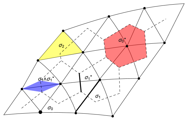
Figure 2.2: A 2-d simplicial complex with points $(\sigma_{0})$, edges ($\sigma_{1}$) and triangles $(\sigma_{2})$ (illustrated in yellow). At each vertex $\sigma_{0}$ there is a dual polytope, $\sigma^{*}_{0}$ (illustrated in red), and at each link, $\sigma_{1}$, there is a dual link $\sigma^{*}_{1}$ and its associated hybrid cell $\sigma_{1}\wedge\sigma^{*}_{1}$ (illustrated in blue).

The construction of our QFE simplicial lattice action can be broken into three steps:

• Simplicial Geometry: The smooth Riemann manifold, $(\mathcal{M},g)$, is replaced by simplex complex, $(\mathcal{M}_{\sigma},g_{\sigma})$ with piecewise flat cells (see Sec. 2.1).

• Classical Lattice Action: The continuum field $\phi(x)$ is replaced by a discrete sum over FEM basis elements, $\phi(x)\rightarrow W^{i}(x)\phi_{i}$ (see Sec. 2.2).

• QFE: Quantum Corrections: Quantum counter terms are added to the discrete lattice action to cancel defects at the UV cut-off (see Sec. 3.2).

2.1 Geometry and Regge Calculus

The Regge Calculus approach to constructing a discrete approximation to a Riemann manifold, $(\mathcal{M},g)$, proceeds as follows. First the manifold, $\mathcal{M}$, is replaced by a simplicial complex, $\mathcal{M}_{\sigma}$, composed of elementary simplicies: triangles in 2d as illustrated in Fig. 2.2, tetrahedrons in 3d, etc. This graph defines the topology of the manifold in the language of Category Theory [20]. Next a discrete metric is introduced as a set of edge lengths on the graph: $g_{\mu\nu}(x)\rightarrow g_{\sigma}=\{l_{ij}\}$. Assuming a piecewise flat interpolation into the interior of each simplex, we now have the Regge representation of a Riemann manifold $(\mathcal{M}_{\sigma},g_{\sigma})$ that is continuous but not differentiable. The curvature is given by a singular distribution at the boundary of the each simplex; in 2d, concentrated at the vertices, and in higher dimensions at the $d\!-\!2$-dimensional “hinges.” The integrated curvature over the defect is easily computed by parallel transport of the tangent vector around each defect.

Each simplex is parameterized by using $d+1$ local barycentric coordinates, $0\leq\xi^{i}\leq 1$. Using the constraint, $\xi^{0}+\xi^{1}+\cdots+\xi^{d}=1$ to eliminate $\xi^{0}$, our $\phi^{4}$ action in Eq. (2.1) on this piecewise flat Regge manifold is given as a sum over each simplex,

$$S\rightarrow S_{\sigma}=\sum_{\sigma\in\mathcal{M_{\sigma}}}\int_{\sigma}d^{d}\xi\sqrt{G_{\sigma}}\left[\tfrac{1}{2}G^{ij}_{\sigma}\partial_{i}\phi(\xi)\partial_{j}\phi(\xi)+\tfrac{1}{2}(m^{2}+\widetilde{\xi}_{0}Ric)\phi^{2}(\xi)+\lambda\phi^{4}(\xi)\right]\;.$$ (2.3)

We may choose an isometric embedding into a sufficiently high dimensional flat Euclidean space with vertices at $\vec{y}=\vec{r}_{n}$ so a point in the interior of each simplex and its induced metric are given by

$$\vec{y}=\sum_{n=0}^{d}\xi^{n}\vec{r}_{n}=\sum_{i=1}^{d}\xi^{i}\vec{l}_{i0}+\vec{r}_{0}\quad,\quad G_{ij}=\frac{\partial{\vec{y}}}{\partial{\xi^{i}}}\cdot\frac{\partial{\vec{y}}}{\partial{\xi^{j}}}\equiv\vec{l}_{i0}\cdot\vec{l}_{j0}\;.$$ (2.4)

This defines the volume element, $\sqrt{G_{\sigma}}=\sqrt{\det[G_{ij}]}$ and inverse metric, $G^{ij}_{\sigma}$, as well.

Since we are not considering dynamical gravity, this piecewise flat metric is frozen (i.e. quenched) and chosen to conform as closely as possible to our target manifold for the quantum field theory. For example this can be achieved by computing the edge length $l_{ij}$, from the proper distance between points on the original manifold $x_{i},x_{j}$ or from the Euclidean distance $|\vec{r}_{i}-\vec{r}_{j}|$ in the isometric embedding space, $\vec{r}_{i}=\vec{y}(x_{i})$ to first order relative to the local curvature of the target manifold. At this stage, the dynamical quantum field $\phi(x)$ is still a continuum function on the piecewise flat Regge manifold.

2.2 Hilbert Space and Discrete Exterior Calculus

The second step is the approximation of the matter field $\phi(x)$ as an expansion,

$$\phi(x)\rightarrow\phi_{\sigma}(\xi)=E^{0}_{\sigma}(\xi)\phi_{0}+E^{1}_{\sigma}(\xi)\phi_{1}+\cdots+E^{d}_{\sigma}(\xi)\phi_{d}\;,$$ (2.5)

into a finite element basis on each simplex $\sigma_{d}$. The simplest form is a piecewise linear function, $E^{i}(\xi)=\xi^{i}$, on each simplex. In this case we are using essentially the same linear approximation for both the metric, $g_{\mu\nu}(x)$, and matter, $\phi(x)$, fields. To evaluate the FEM action, we simply plug the expansion in Eq. (2.5) into Eq. (2.3) and perform the integration. For the kinetic term, this is particularly simple because the gradients of the barycentric coordinates are constant. For 2d, this gives the well known form on each triangle,

$$I_{\sigma} = \frac{l_{31}^{2}+l_{23}^{2}-l_{12}^{2}}{8A_{123}}(\phi_{1}-\phi_{2})^{2}+(23)+(31)$$ (2.6)

$$= \frac{1}{2}A^{(3)}_{12}(\phi_{1}-\phi_{2})^{2}+(23)+(31)$$

where $A^{(3)}_{12}$ is the area of the triangle formed by the sites 1, 2, and the circumcenter, $\sigma_{2}^{*}(123)$. The free scalar action on the entire simplicial complex is now found by summing over triangles,

$$\sum_{\sigma}I_{\sigma}[\phi]=\frac{1}{2}\sum_{\langle ij\rangle}A_{ij}\left(\frac{\phi_{i}-\phi_{j}}{l_{ij}}\right)^{2}\;.$$ (2.7)

Each link $\langle ij\rangle$ receives two contributions—one from each triangle that it borders—resulting in the total area for the hybrid cell, $A_{ij}=l_{ij}|\sigma^{*}_{1}(ij)|/2=\left|\sigma_{1}(ij)\wedge\sigma_{1}^{*}(ij)\right|$, as illustrated in Fig. 2.2.

For higher dimensions, a natural generalization of the kinetic term is

$$S_{\sigma}[\phi]=\frac{1}{2}\sum_{\langle\,i,j\rangle}V_{ij}\frac{(\phi_{i}-\phi_{j})^{2}}{l^{2}_{ij}}+\frac{1}{2}\sum_{i}m\sqrt{g_{i}}\phi^{2}_{i}\;,$$ (2.8)

where $V_{ij}=|\sigma_{1}(ij)\wedge\sigma_{1}^{*}(ij)|=l_{ij}S_{ij}/d$ is the product of the length of the link ($l_{ij}$) times the volume of the $d\!-\!1$-dimensional “surface”, $S_{ij}=|\sigma_{1}^{*}(ij)|$, of the dual polytope normal to the link $\langle\,i,j\rangle$. A mass term has also been included weighted by the dual lattice volume $\sqrt{g_{i}}=|\sigma^{*}_{0}(i)|$. This elegant form was recommended in the seminal papers on random lattices by Christ, Friedberg and Lee [21, 22, 23] and subsequently in the FEM literature by the application of the simplicial Stokes’ theorem for Discrete Exterior Calculus (DEC). However, we note this generalization is not equivalent to linear FEM for $d>2$ (See Ref. [19]).

To appreciate the DEC approach [14, 15, 16, 24], it is useful to expand a little on the geometry of a simplicial complex, $\cal S$, and its Voronorï dual, $\cal S^{*}$. A pure simplicial complex $\cal S$ consists of a set of $d$-dimensional simplices (designated by $\sigma_{d}$) “glued” together at shared faces (boundaries) consisting of $d-$1-dimensional simplices ($\sigma_{d-1})$, iteratively giving a sequence: $\sigma_{d}\rightarrow\sigma_{d-1}\rightarrow\cdots\sigma_{1}\rightarrow\sigma_{0}$. This hierarchy is specified by the boundary operator,

$$\partial\sigma_{n}(i_{0}i_{1}\cdots i_{n})=\sum^{n}_{k=0}(-1)^{k}\sigma_{n-1}(i_{0}i_{1}\cdots\widehat{i}_{k}\cdots i_{n})\;,$$ (2.9)

where $\widehat{i}_{k}$ means to exclude this site. Each simplex $\sigma_{n}(i_{0}i_{1}\cdots i_{n})$ is an anti-symmetric function of its arguments. The signs in Eq. (2.9) keep track of the orientation of each simplex. It is trivial to check that the boundary operator is closed: $\partial^{2}\sigma_{n}=0$. On a finite simplicial lattice $\partial$ is a matrix and its transpose, $\partial^{T}$, is the co-boundary operator. The circumcenter Voronorï dual lattice, $\mathcal{S}^{*}$, is composed of polytopes, $\sigma^{*}_{0}\leftarrow\sigma^{*}_{1}\leftarrow\cdots\leftarrow\sigma^{*}_{d}$, where $\sigma^{*}_{n}$ has dimension $d-n$ as illustrated in Fig. 2.2. A crucial property of this circumcenter duality is orthogonality. Each simplicial element $\sigma_{n}\in S$ is orthogonal to its dual polytope $\sigma^{*}_{n}\in S^{*}$. As a consequence, the volume,

$$|\sigma_{n}\wedge\sigma^{*}_{n}|=\frac{n!(d-n)!}{d!}|\sigma_{n}||\sigma^{*}_{n}|\;,$$ (2.10)

of the hybrid cell, $\sigma_{n}\wedge\sigma^{*}_{n}$, is a simple product. Hybrid cells, constructed from simplices $\sigma_{n}$ in $\cal S$ and their orthogonal dual $\sigma^{*}_{n}$ in $\cal S^{*}$, give a proper tiling of the discrete d-dimensional manifold with the special case $|\sigma_{0}(i)|=1$ and $|\sigma^{*}_{0}(i)|=\sqrt{g_{i}}$. This is a first modest step into discrete homology and De Rham cohomology on a simplicial complex.

The discrete analogue of differential forms, $\omega_{k}$, is a pairing or map,

$$\langle\,\omega_{k},\sigma_{k}\rangle\equiv\omega_{k}(\sigma_{k})=\omega_{k}(i_{0}i_{1}\cdots i_{k})\;,$$ (2.11)

to the numerical value of a field from sites in the case of 0-forms, from links in the case of 1-forms, and from k-simplices in the case of k-forms. Of course this is familiar to lattice field theory, associating scalars ($\omega_{0}\sim\phi_{x}$), gauge fields ($\omega_{1}\sim A_{\mu}dx^{\mu}$) and field strengths ($\omega_{2}\sim F_{\mu\nu}dx^{\mu}\wedge dx^{\nu}$) with sites, links and plaquettes respectively. This enables us to define the discrete analogue of the exterior derivative ${\bf d}\omega_{k}$ of a k-form by replacing the continuum Stokes’ theorem by the discrete map or DEC Stokes’ theorem:

$$\int_{\sigma_{k+1}}{\bf d}\omega(x)=\int_{\partial\sigma_{k+1}}w(x)\quad\rightarrow\quad\langle\,{\bf d}\omega_{k},\sigma_{k+1}\rangle=\langle\,\omega_{k},\partial\sigma_{k+1}\rangle$$ (2.12)

The discrete exterior derivative is automatically closed (${\bf dd}=0$) because the boundary operator is closed ($\partial\partial=0$). Applying Eq. (2.12) to the discrete exterior derivative of a scalar (0-form) field trivially gives,

$$\langle\,{\bf d}\phi,\sigma_{1}(ij)\rangle=\langle\,\phi,\partial\sigma_{1}(ij)\rangle=(\phi_{i}-\phi_{j})\;,$$ (2.13)

the standard finite difference approximation on each link.

Next we need to define the discrete analogue of the Hodge star ($*$). This is the first time an explicit dependence on the metric is introduced. In the continuum, a k-form is an anti-symmetric tensor, $\omega_{k}(x)=(k!)^{-1}\omega_{\mu_{1},\mu_{2}\cdots\mu_{k}}dx^{\mu_{1}}\wedge dx^{\mu_{2}}\wedge\cdots\wedge dx^{\mu_{k}}$, in a orthogonal basis of 1-forms dual to tangent vectors: $dx^{\mu}(\partial_{\nu})=\delta^{\mu}_{\nu}$. The Hodge star takes a k-dimensional basis into its orthogonal complement,

$$*\!(dx^{\mu_{1}}\wedge dx^{\mu_{2}}\wedge\cdots\wedge dx^{\mu_{k}})=dx^{\mu_{k+1}}\wedge dx^{\mu_{k+2}}\wedge\cdots\wedge dx^{\mu_{n}}$$ (2.14)

where $\mu_{1},\mu_{2},\cdots,\mu_{n}$ is an even permutation of $(1,2,\cdots,n)$. However the wedge product (or equivalently the Levi-Civita symbol) is not a tensor but a weight 1 tensor density [25]. The true volume k-form (or tensor), $\mbox{vol}_{k}=\sqrt{g_{k}}dx^{\mu_{1}}\wedge\cdots\wedge dx^{\mu_{k}}$, requires a factor of $\sqrt{g_{k}}$ which under the Hodge star operation in Eq. (2.14) gives the identity, $\sqrt{g_{n\!-\!k}}\;*\!(\mbox{vol}_{k})=\sqrt{g_{k}}\;\mbox{vol}_{n\!-\!k}$, where we have used orthogonality to factor $\sqrt{g}=\sqrt{g_{k}}\sqrt{g_{d-k}}$, that is, between the plane and its dual. Consequently on the simplicial complex, it is reasonable that the proper definition of the discrete Hodge star,

$$\langle\,\omega^{*}_{k},\sigma^{*}_{k}\rangle\;|\sigma_{k}|=\langle\,\omega_{k},\sigma_{k}\rangle\;|\sigma^{*}_{k}|\;,$$ (2.15)

replaces these factors $\sqrt{g_{k}}$, $\sqrt{g_{n\!-\!k}}$ by finite volumes $|\sigma_{k}|$, $|\sigma^{*}_{k}|$ respectively. The Hodge star identity in Eq. (2.15) uniquely fixes the dual field values, $\langle\,\omega^{*}_{k},\sigma^{*}_{k}\rangle$ and the action of a discrete co-differential, $\bm{\delta}=*{\bf d}*$ through Stokes theorem in Eq. (2.12) on $\cal S^{*}$.

Putting this all together, we consider the DEC Laplace-Beltrami operator on scalar fields, $(\bm{\delta}+{\bf d})^{2}\phi=({\bf d}\bm{\delta}+\bm{\delta}{\bf d})\phi=*{\bf d}*{\bf d}\phi$, is

$$*{\bf d}*{\bf d}\phi(i)=\frac{|\sigma_{0}(i)|}{|\sigma^{*}_{0}(i)|}\sum_{j\in\langle\,i,j\rangle}\frac{|\sigma^{*}_{1}(ij)|}{|\sigma_{1}(ij)|}(\phi_{i}-\phi_{j})=\frac{1}{\sqrt{g_{i}}}\sum_{j\in\langle\,i,j\rangle}\frac{V_{ij}}{l_{ij}}\frac{\phi_{i}-\phi_{j}}{l_{ij}}\;,$$ (2.16)

which corresponds to the action in Eq. (2.8). For 2d this is illustrated in Fig. 2.3, as the sum of fluxes through the boundaries $\partial\sigma^{*}_{0}(i)$ with surface area, $S_{ij}/(d-1)!=V_{ij}/l_{ij}=|\sigma_{1}(ij)\wedge\sigma^{*}_{1}(ij)|/l_{ij}$. This is identical to linear finite elements in 2d. Besides providing an alternate approach to linear finite elements for constructing the discrete Hilbert space for scalar fields in $d>2$ dimensions, it provides a useful geometric framework for fields with spin. We note however that additional considerations are still needed for non-Abelian gauge fields [22], Dirac Fermions [19] and Chern-Simons terms [26]. The best geometrization of simplicial field theories and the error estimates thereof are an active research topic.

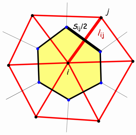
Figure 2.3: The discrete Laplacian at a site $i$ is given by the sum on all links $\langle\,i,j\rangle$ (in red) weighed by gradients $(\phi_{i}-\phi_{j})/l_{ij}$ multiplied by the surface $S_{ij}=2V_{ij}/l_{ij}$ (in black) and normalized by the dual volume $|\sigma^{*}_{o}(i)|=V_{i}$ (in yellow).

To complete the simplicial action, we need to add the potential term. This may be constructed in a variety of ways. If one follows strictly the linear finite element prescription, the expression for the local polynomial potential (e.g. mass and quartic terms) will not be local but rather point split on each simplex $\sigma_{d}$. For example, in 2d, after expanding $\phi(\xi)=\sum^{d}_{i=0}\xi^{i}\phi_{i}$ and evaluating the integral over the linear elements, the contribution for the quadratic term on a single triangle, $\sigma_{2}(123)$, is

$$\int_{\sigma}d^{2}\xi\sqrt{G_{\sigma}}\phi^{2}_{\sigma}(\xi)=\frac{A_{123}}{6}(\phi^{2}_{1}+\phi^{2}_{2}+\phi^{2}_{3}+\phi_{1}\phi_{2}+\phi_{2}\phi_{3}+\phi_{3}\phi_{1})\;.$$ (2.17)

The general expression for a homogeneous polynomial over a d-simplex with volume $V_{d}=|\sigma_{d}|$ is given as as sum over distinct partitions of $n$:

$$\int_{\sigma_{d}}dV_{d}\;(\phi(\xi))^{n}=\frac{V_{d}\;d!\;n!}{(n+d)!}\sum_{(\sum_{i}k_{i}=n)}\phi_{0}^{k_{0}}\phi_{1}^{k_{1}}\cdots\phi_{d}^{k_{d}}\;.$$ (2.18)

Nonetheless in the spirit of dropping higher dimensional operators in a derivative expansion, we choose local terms approximating the potential at each vertex weighted by the volume , $\sqrt{g_{i}}=|\sigma^{*}_{0}(i)|$, of the dual simplex $\sigma^{*}_{0}(i)$.

This approximation leads to our complete simplicial action, combining the DEC Laplace-Beltrami operator for the kinetic term and the local approximation for the boundary,

$$S=\frac{1}{2}\sum_{\langle ij\rangle}\frac{V_{ij}}{l_{ij}^{2}}(\phi_{i}-\phi_{j})^{2}+\lambda_{0}\sum_{i}\sqrt{g_{j}}\left(\phi_{i}^{2}-\frac{\mu^{2}_{0}}{2\lambda_{0}}\right)^{2}+h\sum_{i}\sqrt{g_{i}}\phi_{i}\;,$$ (2.19)

where $\mu^{2}_{0}=-m^{2}_{0}/2$. We will use this action for our discussion of ${\mathbb{S}}^{2}$.

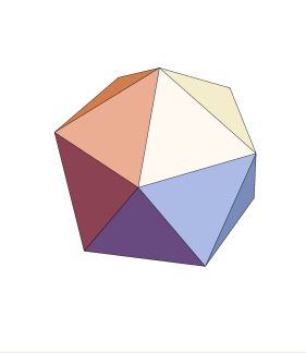
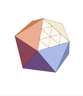
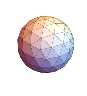
Figure 2.4: The $L=3$ refinement of the icosahedron with $V=2+10L^{2}=92$ vertices or sites. The icosahedron on the left is refined in the middle with $L^{2}=9$ equilateral triangles on each face, and then on the right the new vertices are projected onto the unit sphere. The resulting simplicial complex preserves the icosahedral symmetries.

Finally we should acknowledge that there are many other alternatives in the FEM literature worthy of consideration which may offer improved convergence and faster restoration of the continuum symmetries. Our goal here is to find the simplest discrete action on simplicial lattice capable of reaching the correct continuum theory with no more fine tuning than is required on the hypercubic lattice.

2.3 Spectral Fidelity on ${\mathbb{S}}^{2}$

We represent $\mathbb{S}^{2}$ embedded in $\mathbb{R}^{3}$ parameterized by 3-d unit vectors:

$$\hat{r}=(r_{x},r_{y},r_{z})\in\mathbb{R}^{3}\quad,\quad r^{2}_{x}+r^{2}_{y}+r^{2}_{z}=1\;.$$ (2.20)

In order to preserve the largest available discrete subgroup of $O(3)$, we start with the regular icosahedron illustrated on the left in Fig. 2.4 and subsequently divide each of the 20 equilateral triangles into $L^{2}$ smaller equilateral triangles. Then we project the vertices radially outwards onto the surface of the circumscribing sphere, dilating and distorting each triangle from its equilateral form, but preserving exactly the icosahedral symmetries. The total numbers of faces, edges, and vertices are $F=20L^{2}$, $E=30L^{2}$ and $N=2+10L^{2}$, respectively, satisfying the Euler identity $F-E+N=2$.

The images of the vertices on the sphere are then connected by new links consistent with the unique Delaunay triangulation [27]. In the triangulation, each vertex is connected to five or six neighboring vertices by edges $\langle\,x,y\rangle$. The lengths are set to the secant lengths $l_{xy}=|\hat{r}_{x}-\hat{r}_{y}|$ in the embedding space between the vertices on the sphere, which approximates the geodesic length to $O(l^{2}_{xy})$. The extension to a lattice for the ${\mathbb{R}}\times{\mathbb{S}}^{2}$ cylinder introduces a uniform (periodic) lattice perpendicular to the spheres at $t=0,1,\cdots,L_{t}-1$. The sequence of refinements as $L\rightarrow\infty$ divides the total curvature into vanishingly small defects at each vertex. As an alternative formulation, we could replace the flat triangles with spherical triangles [28], introducing spherical areas, geodesic lengths, moving the curvature uniformly into the interior of each triangle. In this formulation, each triangle would have a vanishing deficit angle in the continuum limit. Both discretizations are equivalent at $O(a^{2})$, and as such we prefer flat triangles due to their relative simplicity.

The first test of our construction is to look at the spectrum of the free theory,

$$S_{0}=\frac{1}{2}\phi_{x}M_{x,y}\phi_{y}=\frac{A_{xy}}{2l^{2}_{xy}}(\phi_{x}-\phi_{y})^{2}+\frac{m^{2}_{0}}{2}\sqrt{g_{x}}\phi^{2}_{x},$$ (2.21)

where $x,y=1,...,N$ enumerates the lattice sites on a finite simplicial lattice. The spectrum is computed from the generalized eigenvalue condition

$$M_{xy}\phi_{n}(x)=E_{n}\sqrt{g_{x}}\phi_{n}(x)=(E^{(0)}_{n}+m^{2}_{0})\sqrt{g_{x}}\phi_{n}(x),$$ (2.22)

where the eigenvalues at zero mass are $E^{(0)}_{n}$. Each distinct eigenvalue $E_{n}$ has right/left generalized eigenvectors, $\phi_{n}(x)/\phi^{*}_{n}(x)$, with the orthogonality and completeness relations,

$$\sum_{x}\sqrt{g_{x}}\phi^{*}_{n}(x)\phi_{m}(x)=\delta_{nm}\quad,\quad\sum_{n}\phi^{*}_{n}(y)\phi_{n}(x)=\delta_{xy}/\sqrt{g_{x}}\;.$$ (2.23)

The spectral decomposition for the free propagator is

$$G_{xy}(m^{2}_{0})\equiv\left[\frac{1}{M}\right]_{xy}=\sum_{n}\frac{\phi_{n}(x)\phi^{*}_{n}(y)}{E^{(0)}_{n}+m^{2}_{0}}$$ (2.24)

Alternatively we may define a Hermitian form, $\widetilde{M}=g^{-1/4}Mg^{-1/4}$, with complex conjugate right and left eigenvectors, $g_{x}^{1/4}\phi_{n}(x)=\langle\,x|n\rangle$ and $\phi^{*}_{n}(x)=\langle\,n|x\rangle$, respectively. In Dirac notation the completeness and orthogonality are given by ${\bf 1}=\sum_{x}|x\rangle\langle\,x|$ , ${\bf 1}=\sum_{n}|n\rangle\langle\,n|$ and $\delta_{x,y}=\langle\,x|y\rangle$, $\delta_{n,m}=\langle\,n|m\rangle$ respectively.

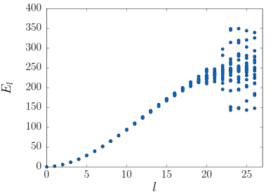
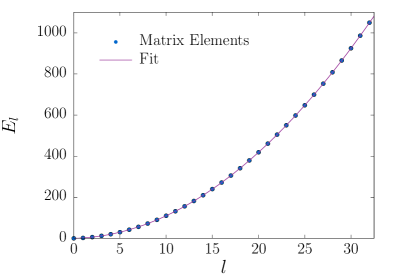
Figure 2.5: Left: The $2l+1$ spectral values for $m\in[-l,l]$ are plotted against $l$ for $L=8$. Right: The spectral values averaged over $m$ fitted to $l+1.00002\;l^{2}-1.27455\times 10^{-5}\;l^{3}-5.58246\times 10^{-6}\;l^{4}$ for $L=128$ and $l\leq 32$.

Returning to the example of the FEM sphere, ${\mathbb{S}}^{2}$, we have verified that the generalized eigenvalues which lie well below the cut-off are well fitted by the continuum spectrum, $E_{lm}=l(l+1)$, with the $2l+1$ degeneracy $m=-l,\cdots l$. Indeed, any finite eigenvalue approaches its continuum value as $1/L^{2}$ in the limit of infinite refinement $L\rightarrow\infty$. In addition, we note that the right eigenvectors are well approximated by the continuum spherical harmonics, $Y_{lm}(\hat{r}_{x})$, evaluated at the lattice sites $\hat{r}_{x}$. This is illustrated in Fig. 2.5, where the eigenvalues are estimated by computing diagonal matrix elements,

$$E_{l,m}=\frac{Y^{*}_{lm}(\hat{r}_{x})M_{xy}Y_{lm}(\hat{r}_{y})}{\sum_{x}\sqrt{g_{x}}Y^{*}_{lm}(\hat{r}_{x})Y_{lm}(\hat{r}_{x})}\;,$$ (2.25)

against $l$. On the left of Fig. 2.5, the lack of $2l+1$ degenerate multiplets on a coarse lattice with $L=8$, as we approach the cut-off at large $l\sim O(L)$, shows the breakdown of rotational symmetry. On the right of Fig.2.5, the degeneracy of the spherical representation holds to high accuracy and the average of the $2l+1$ eigenvalues at each $l$ level gives the correct continuum dispersion relation, $l(l+1)$, to $O(10^{-5})$ for $l\ll L=128$.

We will refer to the exact convergence of fixed eigenvalues and their associated eigenvectors to the continuum as the cut-off is removed as spectral fidelity. This is a theoretical consequence of FEM convergence theorems for shape regular linear elements as the diameter goes uniformly to zero [13]. We do not provide a proof but will assume that this property holds for our implementation if we apply the DEC [15] to the Laplace-Beltrami operator.

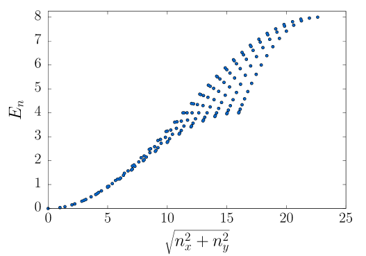
Figure 2.6: The zero mass spectrum $E_{n}=4(\sin^{2}(k_{x}/2)+\sin^{2}(k_{y}/2))$, $k_{\mu}=\frac{n_{\mu}\pi}{L}$, $n_{\mu}\in\left[-L/2,L/2-1\right]$ for the 2-d lattice Laplacian on a regular $32\times 32$ square lattice plotted against $\sqrt{n^{2}_{x}+n^{2}_{y}}$.

It is useful to compare the low spectrum of our FEM operator on ${\mathbb{S}}^{2}$, shown in Fig. 2.5, to the corresponding spectrum on the hypercubic refinement of the torus ${\mathbb{T}}^{2}$, shown in Fig. 2.6. For a finite $L^{d}$ toroidal lattice, the exact hypercubic spectra is given by

$$E_{n}=\sum_{\mu}4\sin^{2}(k_{\mu}/2)+m^{2}_{0}\simeq m^{2}_{0}+\sum_{\mu}[k^{2}_{\mu}-\frac{1}{12}k^{4}_{\mu}+\cdots],$$ (2.26)

where the discrete eigenvalues are enumerated by $k_{\mu}=2\pi n_{\mu}/L$ for integer $n_{\mu}\in[-L/2,L/2-1]$. The eigenvectors can be found by a Fourier analysis, and are given by

$$\phi_{n}(x)=\frac{1}{\sqrt{N}}e^{-ik\cdot x}\quad,\quad\phi^{*}_{n}(x)=\frac{1}{\sqrt{N}}e^{ik\cdot x}\;.$$ (2.27)

Converting to dimensionful variables ($m,p$) and holding a physical mass fixed ($m\equiv m_{0}/a$), the dispersion relation is $a^{2}E_{n}=m^{2}+p^{2}-\frac{1}{12}\sum_{\mu}a^{2}p^{4}_{\mu}+\cdots$. The Lorentz breaking term vanishes as $a^{2}=O(1/L^{2})$. Again spectral fidelity holds for any fixed spectral value $E_{n}$ as the lattice converges to the continuum. However, as we approach the cut-off, it is increasingly distorted.

Clearly the spectral fidelity on the hypercubic torus is comparable to the FEM spectra on ${\mathbb{S}}^{2}$. This is not surprising; indeed the square lattice can also be viewed as a FEM realization. One simply divides each square into two right angle triangles and notices that the formula in Eq. (2.8) implies a zero contribution on the diagonal links. This generalizes to higher dimensional hypercubic lattices when using the DEC form. Of course, the major difference between the square lattice on ${\mathbb{R}}^{2}$ and the simplicial sphere ${\mathbb{S}}^{2}$ is the former breaks one rotational isometry of the continuum but conserves two discrete subgroups of translations, whereas the later breaks all three isometries of $O(3)$ down to a fixed finite subgroup independent of the refinement.

2.4 Obstruction to Non-Linear Quantum Path Integral

Having demonstrated the spectral fidelity of our construction on ${\mathbb{S}}^{2}$ at the Gaussian level, we turn next to the more difficult problem of an interacting quantum theory, starting with the FEM action given in Eq. (2.19). We have performed extensive Monte Carlo simulations for the path integral given the FEM action in Eq. (2.19) on ${\mathbb{S}}^{2}$ with a conclusive result: the FEM action does not converge to a spherically symmetric theory as you approach the continuum and fails to have a well defined critical surface. Attempting to locate the critical surface, we monitor the Binder cumulant. The results are given on the left-hand side of Fig. 2.7. As we increase the cut-off (or $L\rightarrow\infty$) while tuning the only relevant coupling, $\mu^{2}_{0}$, the fourth Binder cumulant should stabilize to the known, exact value $U^{*}_{4}=0.8510207(63)$ for the Ising CFT (see Sec. 4 for details). Instead we see that there is an alarming instability at large $L=O(100)$, which we believe is due to the lack of well-defined critical surface with a second order phase transition required to define a continuum limit. A more graphic indication of this failure is present when we consider the average value of $\langle\,\phi^{2}_{i}\rangle$ as a function of position on the sphere as shown on the right-hand side of Fig. 2.7. Due to a spatial variation in the UV cut-off, this is not uniform, with variation that can be seen by comparing the regions close to and far form the 12 exceptional five-fold vertices of the original icosahedron. As we will show, this failure is also evident in a lattice perturbation expansion. At small $\lambda_{0}$ a spherically asymmetric contribution to $\langle\,\phi^{2}_{i}\rangle$ is given by a UV divergent one-loop diagram.

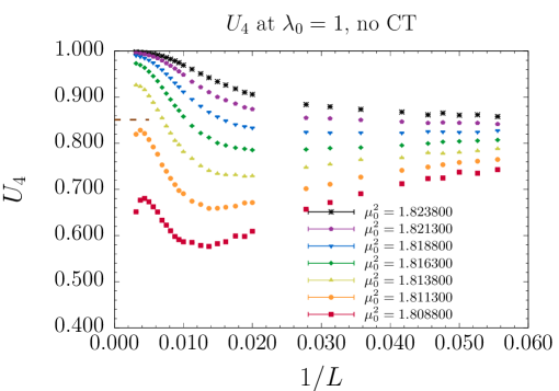
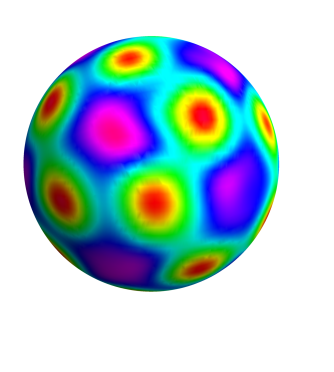
Figure 2.7: On the left the Binder cumulants for the FEM Lagrangian with no QFE counter term. On the right the amplitude of $\langle\,\phi^{2}_{i}\rangle$ in simulations with the unrenormalized FEM Lagrangian.

In conclusion, in the application of FEM to quantum field theory, we have encountered a fundamentally new problem. The FEM methodology has been developed to give a discretization for non-linear PDEs that converges to the correct continuum solution as the simplicial complex is refined. In the context of a Lagrangian system for a quantum field, this implies a properly implemented FEM should therefore guarantee convergence to all smooth classical solutions of the EOM as the cut-off is removed. However, quantum field theory is more demanding. The path integral for an interacting quantum field theory is sensitive to arbitrarily large fluctuations—even in perturbation theory—on all distance scales, down to the lattice spacing, due to ultraviolet divergences. This amplifies local UV cut-off effects on our FEM simplicial action.

Our solution is to introduce a new Quantum Finite Element (QFE) lattice action that includes explicit counter terms to regain the correct renormalized perturbation theory. We conjecture that, for any ultraviolet complete theory, if the QFE lattice Lagrangian is proven to converge to the continuum UV theory to all orders in perturbation theory, this is sufficient to define its non-perturbative extension to the IR. We believe this is a plausible conjecture consistent with our experience on hypercubic lattices for field theories in ${\mathbb{R}}^{d}$, but it is far from obvious. It needs careful theoretical and numerical support to determine its validity. In Sec. 4 and Sec. 5 we give extensive numerical test for $\phi^{4}$ on ${\mathbb{S}}^{2}$ on the critical surface. In particular the new Monte Carlo simulation of the Binder cumulant $U_{4}$ on the right hand side of Fig. 4.1 including the quantum counter term gives a critical value of the Binder cumulant, $U_{4,\mathrm{cr}}=0.85020(58)(90)$, in agreement with the continuum value, $U^{*}_{4}=0.8510$, to about one part in $10^{3}$. While this is promising, the limitations due to statistics and the restriction of our studies to the simplest scalar 2-d CFT is duly acknowledged.

3 Ultraviolet Counter Terms on the Simplicial Lattice

To remove the quantum obstruction to criticality for the FEM simplicial action, we begin by asking if we can add counter terms to the action Fig. 2.19 to reproduce the renormalized perturbation expansion order by order in the continuum limit at the UV weak coupling fixed point. On a hypercubic lattice, it has been proven for $\phi^{4}$ theory [29] that this can be achieved by taking the lattice UV cut-off to infinity, holding the renormalized mass and coupling fixed. Here we will suggest how this can be achieved on a simplicial lattice for 2d and 3d. While we do not attempt a proof, the similarity with the hypercubic example strongly suggests that a proof could be found at the expense of increased technical difficulty.

The $\phi^{4}$ theory is super-renormalizable in 2d and 3d, with one-loop and two-loop divergent diagrams, respectively, only contributing to the two-point function. The one-loop diagram is logarithmically divergent in 2d and linearly divergent in 3d. The two-loop diagram is UV finite in 2d, but logarithmically divergent in 3d. The divergent contributions renormalize the mass via the one-particle irreducible (1PI) contribution to the self-energy,

$$\Sigma(x,y)=-12\lambda_{0}G_{0}(x,y)\delta(x-y)+96\lambda^{2}_{0}G^{3}_{0}(x,y)\;,$$ (3.1)

as illustrated in the first two panels in Fig. 3.1. In both 2d and 3d the three-loop diagram, and all higher-order diagrams, are UV finite. In 4d there is a logarithmically divergent contribution to the four-point function which contributes to the quartic coupling $\lambda_{0}$; however the complete non-perturbative theory is the trivial free theory with no interesting IR physics.

3.1 Lattice Perturbation Expansion

The perturbation expansion for the $\phi^{4}$ theory on our FEM lattice (or indeed any lattice) starts with the partition function,

$$Z(m_{0},\lambda_{0})=\int{\cal D}\phi_{i}e^{-\textstyle\frac{1}{2}\phi_{i}M_{i,j}\phi_{j}-\lambda_{i}\phi^{4}_{i}}\;,$$ (3.2)

by expanding in the quartic term. In our FEM representation, the action is

$$S[\phi_{i}]=\frac{1}{2}\phi_{i}M_{i,j}\phi_{j}+\lambda_{i}\phi^{4}_{i}=\frac{1}{2}[\phi_{i}K_{i,j}\phi_{j}+m_{i}^{2}\phi^{2}_{i}]+\lambda_{i}\phi^{4}_{i}\;.$$ (3.3)

For convenience, both bare parameters $m_{i}^{2}\equiv\sqrt{g_{i}}m_{0}^{2}$ and $\lambda_{i}\equiv\sqrt{g_{i}}\lambda_{0}$ include the factor of the local dual volume $\sqrt{g_{i}}$. The quadratic form ($M_{i,j}$) includes both the DEC Laplace-Beltrami operator ($K_{i,j}$) and the bare mass ($m_{0}$).

Following the standard Feynman rules for a perturbative expansion in $\lambda_{0}$, we compute the propagator, $\langle\,\phi_{i}\phi_{j}\rangle=Z^{-1}\int{\cal D}\phi\;\phi_{i}\phi_{j}e^{-S}$, to second order:

$$\langle\,\phi_{i}\phi_{j}\rangle=\left[M^{-1}\right]_{i,j} +\left[M^{-1}\right]_{i,i_{1}}(-12\lambda_{i_{1}}\left[M^{-1}\right]_{i_{1},i_{1}})\left[M^{-1}\right]_{i_{1},j}$$

$$+\left[M^{-1}\right]_{i,i_{1}}(96\lambda_{i_{1}}\lambda_{i_{2}}\left[M^{-1}\right]^{3}_{i_{1},i_{2}})\left[M^{-1}\right]_{i_{2},j}\;.$$ (3.4)

After amputating the external lines, we find the inverse propagator $\widetilde{M}_{ij}(m_{0},\lambda_{0})=M_{i,j}+\Sigma_{ij}(m_{0},\lambda_{0})$, where

$$\Sigma_{ij}(m_{0},\lambda_{0})=-12\lambda_{i}\left[M^{-1}\right]_{ii}\delta_{ij}+96\lambda_{i}\lambda_{j}\left[M^{-1}\right]^{3}_{i,j}+O(\lambda^{3}_{0})\;.$$ (3.5)

is the 1PI simplicial self-energy.

Figure 3.1: The one-loop diagram is logarithmically divergent in 2d and linearly divergent in 3d, whereas the two-loop is finite and logarithmically divergent for 2d and 3d, respectively. The three-loop diagram is finite in both 2d and 3d.

3.2 One Loop Counter Term

Since there is no analytic spectral representation of the free FEM Green’s function, we compute the one loop diagram in co-ordinate space by numerical evaluation of the propagator. To be concrete, for 2d on ${\mathbb{S}}^{2}$ and for 3d on ${\mathbb{R}}\times{\mathbb{S}}^{2}$, the Gaussian term is

$$\phi_{x,t_{1}}M_{x,t_{1};y,t_{2}}\phi_{y,t_{2}}=\phi_{x,t_{1}}K_{x,y}\phi_{y,t_{1}}+\sqrt{g_{x}}(\phi_{x,t}-\phi_{x,t\pm 1})^{2}+m^{2}_{0}\sqrt{g_{x}}\phi^{2}_{x,t}\;,$$ (3.6)

where the sites are now labeled by $i=(x,t)$. The 2-d geometry, ${\mathbb{S}}^{2}$, can be viewed as a special case with a single sphere at $t=0$. The integer $t$ labels each sphere along the cylinder, and $x$ indexes the sites on each sphere. $K_{x,y}$ is non-zero on only nearest neighbor links $\langle\,x,y\rangle$. To take the continuum limit we need to define the normalization convention of our lattice constants:

$$\sum^{N-1}_{x=0}\sqrt{g_{x}}=N\quad\mbox{and}\quad\sum_{\langle\,x,y\rangle}K_{x,y}=(2/3)E\;,$$ (3.7)

where in this specific context $E$ refers to the number of edges on the simplicial graph. The extra factor of $2/3$ is introduced to compensate, on average, for the six nearest neighbors per site on the sphere relative to a conventional square lattice with four nearest neighbors. In flat 2-d space this factor of 2/3 for the triangular lattice gives the same dispersion relation, $E=m^{2}_{0}+k^{2}+O(k^{4})$, as the square lattice.

In lattice perturbation theory on a 2-d FEM simplicial lattice, we expect the logarithmically divergent one-loop term to give a site-dependent mass shift,

$$m^{2}_{0}\rightarrow m^{2}_{0}+\Delta m_{x}^{2}\;.$$ (3.8)

The numerical computation of the one-loop diagram on ${\mathbb{S}}^{2}$ does indeed have the appropriate form,

$$\left[M^{-1}\right]_{xx}\approx\frac{\sqrt{3}}{8\pi}\log\left(\frac{1}{m^{2}a_{x}^{2}}\right)=\frac{\sqrt{3}}{8\pi}\log(N)+\frac{\sqrt{3}}{8\pi}\log\left(\frac{a^{2}}{a_{x}^{2}}\right)+O(1/N)\;.$$ (3.9)

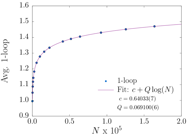
Figure 3.2: The numerical fit of the lattice one loop log divergent determining coefficient $Q$ compared to the continuum value: $Q=\sqrt{3}/(8\pi)=0.0689161\cdots$.

The logarithmic divergence is regulated by the IR mass, $m^{2}$. Of course on the lattice, at fixed dimensionless bare mass, $m^{2}_{0}=a^{2}m^{2}$ and bare coupling, $\lambda_{0}$, there is no actual UV divergence. The renormalized perturbation expansion is defined by fixing the physical mass ($m$), which in the continuum limit ($N\rightarrow\infty$) corresponds to a vanishing effective lattice spacing, $a^{2}m^{2}=O(1/N)$. On a hypercubic lattice, there is a universal cut-off ($\pi/a_{x}=\pi/a$), whereas on a simplicial lattice the one-loop term separates into two terms on the right side of Eq. (3.3): (1) a position independent divergence and (2) a finite (scheme dependent) constant for each site $x$.

We have checked numerically, to high accuracy, that the first divergent term is independent of position. This is a crucial observation which we believe is a general consequence of the FEM prescription. Spatial dependence for a divergent term would imply the need for a divergent counter term to restore spherical symmetry. This departs from the standard cut-off procedure on regular lattices and would be very difficult if not impossible to implement. Moreover, we show in Fig. 3.2 that the fit coefficient is accurately determined to be $\sqrt{3}/(8\pi)$, which is the exact continuum value.

A heuristic argument for the value of this constant follows from our ${\mathbb{S}}^{2}$ tessellation as a nearly regular triangular lattice. In flat space, relative to a square lattice, the density of states on a triangular lattice is $N^{-1}\sum_{n}\rightarrow\int d^{2}k~{}\rho_{T}(k)$, where $\rho_{T}=\sqrt{3}/(8\pi^{2})$. The extra factor of $\sqrt{3}/2$ is due to the area $|\sigma^{*}_{0}|$ of the dual lattice hexagon relative to the dual lattice square on a hypercubic lattice. However, since this constant defines the local charge in the 2-d Coulomb law and our linear elements do not implement local flux conservation, this is surprising result. Nonetheless in Sec. 3.3 we will prove this based on the FEM principle of spectral fidelity and the renormalization group for the mass anomalous dimension. To the best of our knowledge this is a novel extension of FEM convergence theorems.

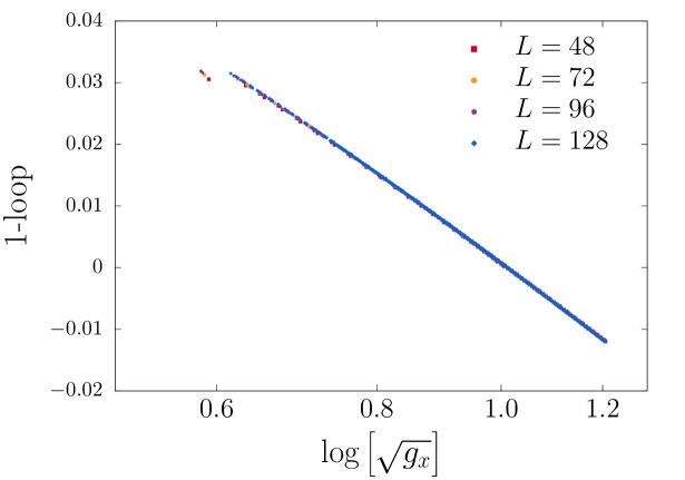
Figure 3.3: One Loop counter term plotted against $\log(\sqrt{g_{x}})$.

Next consider the finite spatial dependence term in Eq. (3.9). As illustrated in Fig. 3.3, it is almost exactly a linear function of $\log[\sqrt{g_{x}}]$. Again there is a heuristic explanation for this. An almost perfect analytic expression can be found by considering the dilatation incurred by the projection of our triangular tessellation of the icosahedron onto the sphere. The icosahedron is a manifold with a flat metric except for 12 conical singularities at the vertices. Our choice of the simplicial complex began with flat equilateral triangles on each of the 20 faces of the original icosahedron. The radial projection onto the sphere is a Weyl transformation to constant curvature with conformal factor (or Jacobian of the map),

$$\sqrt{g(x)}=e^{\sigma(x)}=\frac{(x^{2}_{1}+x^{2}_{2}+1-R_{c}^{2})^{3/2}}{\sqrt{1-R_{c}^{2}}}\;,$$ (3.10)

where $R_{c}$ is the circumradius for one of the 20 icosahedral faces and $x_{1},x_{2}$ the flat coordinates on that face. This formula gives a line coinciding with the linear data in Fig. 3.3. Although this is an extremely good approximation to the counter term, it is not perfect since it neglects the conical singularities in the map near the 12 exceptional vertices of the original icosahedron. These exceptional points are visible in the upper left corner of Fig. 3.3. We find that the true numerical computation does give better results and, moreover, it is a general method not requiring our careful triangulation procedure. A more irregular procedure should also be allowed. The lesson is that the simplicial metric, $g_{ij}=\{l_{ij}\}$, on a given Regge manifold not only defines the intrinsic geometry but also a co-ordinate system breaking diffeomorphism explicitly. The set of lengths includes both a definition of curvature and the discrete co-ordinate system. The counter term must compensate for this arbitrary choice.

The QFE one loop counter term is introduced to cancel the finite position dependence in Eq. (3.9) that violates rotational invariance to order $\lambda_{0}$. To project out the spherical component of a local scalar density, $\rho_{x}$, we average over the rotation group $R\in SO(3)$,

$$\frac{1}{\mbox{vol}O(3)}\int dR\;\rho(R\hat{r})=\frac{1}{4\pi}\int d\Omega\;\rho(\theta,\phi)\simeq N^{-1}\sum_{x}\sqrt{g_{x}}\rho_{x}\;.$$ (3.11)

Applied to $\rho_{x}=\left[M^{-1}\right]_{xx}$, the subtracted lattice Green’s function is

$$\delta G_{xx}=\left[M^{-1}\right]_{xx}-\frac{1}{N}\sum_{x=1}^{N}\sqrt{g_{x}}\left[M^{-1}\right]_{xx}.$$ (3.12)

This removes completely the logarithmic divergence, leaving the position dependent finite counter term which adds a contribution to the FEM action,

$$S_{FEM}\rightarrow S_{QFE}=S_{FEM}+6\sum_{x}\sqrt{g_{x}}\lambda_{0}\;\delta G_{xx}\;\phi^{2}_{x}\;.\$$ (3.13)

In 2d $\phi^{4}$ theory this is the only UV divergent term. We also computed the two-loop contribution to the 1PI simplicial self energy Eq. (3.5) which in co-ordinate space is given by the third power of the Green’s function, $\left[M^{-1}\right]^{3}_{xy}$, between the vertex at $x$ and $y$. The position dependence,

$$\delta\left[G_{x}\right]^{3}=\sum_{y}(\left[M^{-1}\right]^{3}_{xy}-\frac{1}{N}\sum_{x=1}^{N}\sqrt{g_{x}}\left[M^{-1}\right]^{3}_{xy})\;,$$ (3.14)

is found again by subtracting the average contribution on the sphere. The result is plotted in Fig. 3.4, against $\log[\sqrt{g_{x}}]$ which demonstrates that it vanishes rapidly in the continuum limit as $1/L^{2}\sim 1/N$ consistent with naïve power counting in continuum perturbation theory.

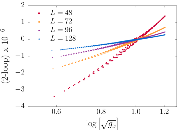
Figure 3.4: The contribution of the two loop term in 2d.

While we do not attempt a general analysis of the simplicial lattice perturbation expansion, it is plausible based on analogous studies on the hypercubic lattice [30, 31] that after canceling cut-off dependence in the one loop UV divergent term the entire expansion restores the renormalized perturbation series in the continuum limit. However our test on the 2-d Riemann sphere simplicial lattice goes further. Namely we give numerical evidence that this 2-d QFE lattice action, when tuned to the the critical surface, approaches the non-perturbative continuum theory in the IR for the Ising CFT field theory.

3.3 Universal Logarithmic Divergence

The success of our QFE action prescription depends on the coefficient of the logarithmic divergence being exact in the continuum limit. On ${\mathbb{S}}^{2}$ or any maximally symmetric space, this implies the coefficient is also independent of position. At first, this observation appears surprising. After all, the UV divergence is sensitive to the local, short distance cut-off which is not uniform. We claim this is a consequence of the observed spectral fidelity of the DEC Laplace-Beltrami operator and renormalization group (RG) for a logarithmic divergence relating UV divergences to the IR regulator. Adapting the argument to a general 2-d Riemann manifold is in principle straight forward, matching the local divergence to the one loop renormalization of the continuum theory [7] at each point $x$.

Let us first apply this renormalization group (RG) argument to the hypercubic lattice, where we already know and understand the answer. Suppose that the one-loop diagram has a logarithmic term,

$$G_{xx}(m)\simeq c_{x}log(1/m^{2}a^{2}_{x})+O(a^{2}m^{2})\;.$$ (3.15)

with an unknown position dependent coefficient $c_{x}$. To isolate this coefficient, we take the logarithmic derivative, finding

$$\gamma_{1}(m^{2})=-m\frac{\partial}{\partial m}G_{xx}(m^{2})=2\iint^{\pi/a}_{-\pi/a}\frac{d^{2}p}{(2\pi)^{2}}\frac{m^{2}}{(4a^{-2}\sum_{\mu}\sin^{2}(ap_{\mu}/2)+m^{2})^{2}}\;.$$ (3.16)

so that $\gamma_{1}(m^{2})=2c_{x}+O(a^{2}m^{2})$. This is the one-loop contribution to the anomalous dimension of the $\phi^{2}$ operator. (To clarify scaling, we have re-introduced the lattice spacing $a$ so that $p=k/a,m=m_{0}/a$ have mass dimensions.) By power counting, the integral resulting from the logarithmic derivative is UV finite in the continuum limit. We may now introduce a new cut-off, $\Lambda_{0}$, separating the IR from the UV: $m\ll\Lambda_{0}\ll\pi/a$. To estimate the integral, we can take the continuum limit $\pi/a\rightarrow\infty$,

$$\gamma_{1}(m^{2})\simeq 2\iint^{\Lambda^{2}_{0}}_{0}\frac{dp^{2}}{4\pi}\frac{m^{2}}{(p^{2}+m^{2})^{2}}+O(m^{2}/\Lambda^{2}_{0})=\frac{1}{2\pi}\frac{1}{1+m^{2}/\Lambda^{2}_{0}}+O(m^{2}/\Lambda^{2}_{0})\;,$$ (3.17)

followed by taking the IR regulator to zero: $m^{2}/\Lambda^{2}_{0}\rightarrow 0$. This proves that the coefficient $c_{x}=1/(4\pi)$ is independent of position and identical to the continuum value on ${\mathbb{R}}^{2}$. Of course, this is not surprising for flat space.

Now we can apply the same reasoning to the simplicial sphere ${\mathbb{S}}^{2}$, beginning with the spectral representation of the Green’s function,

$$G_{xx}(m^{2})=\sum_{n}\frac{\phi^{*}_{n}(x)\phi_{n}(x)}{E^{(0)}_{n}+m^{2}_{0}}\;.$$ (3.18)

On the basis of FEM spectral fidelity, assume the low eigenspectrum for $l\leq L_{0}$ is well approximated to $O(1/N)$ by spherical harmonics,

$$E_{n}\simeq a^{2}R^{-2}l(l+1)+m^{2}_{0}\quad,\quad\phi_{n}(x)\simeq\frac{\sqrt{4\pi}}{\sqrt{N}}Y_{lm}(\hat{r}_{x})\;,$$ (3.19)

where $R/a$ is the radius of the sphere in units of the lattice spacing. Matching the area of the sphere with $N$ triangles we have $4\pi R^{2}=a^{2}N\sqrt{3}/2$. For $R=1$ the spectrum is $l(l+1)$, but with our convention of setting $a=1$, we find $R=\sqrt{3}N/(8\pi)$. Next, we fix the eigenvector normalization by requiring $\sum_{x}\sqrt{g_{x}}|Y_{00}|^{2}=N/4\pi$.

By splitting the spectral sum at the cut-off $L_{0}$, and using the addition formula, $4\pi\sum_{m}Y^{*}_{lm}(\hat{r}_{x})Y_{lm}(\vec{r}_{y})=(2l+1)P_{l}(r_{x}\cdot r_{y})$ for $l<L_{0}$, we have

$$G_{xy}(m^{2}_{0})\simeq\frac{\sqrt{3}}{8\pi}\sum^{L_{0}}_{l=0}\frac{(2l+1)P_{l}(r_{x}\cdot r_{y})}{l(l+1)+\mu^{2}}+\sum^{N}_{n=(L_{0}+1)^{2}}\frac{\phi^{*}_{n}(x)\phi_{n}(y)}{E^{(0)}_{n}+m^{2}}\;,$$ (3.20)

where we introduced $\mu^{2}=R^{2}(m^{2}_{0}/a^{2})$. The first term is indeed rotationally invariant. At $x=y$, the asymptotic limit of the first term is $\sqrt{3}\log(L_{0})/(8\pi)$, which is the desired behavior. As with the infinite, flat lattice, we wish to convert the sum of the first term to an integral in the limit $N\rightarrow\infty$:

$$\sum_{l}\rightarrow\int dE\rho(E)\quad,\quad\rho(E)=\frac{dl}{dE_{n}}=\frac{R^{2}}{2l+1}$$ (3.21)

so that

$$G_{xx}(m^{2}_{0})\simeq\frac{\sqrt{3}}{8\pi}\sum^{L_{0}}_{l=0}\frac{(2l+1)}{l(l+1)+\mu^{2}}\rightarrow\frac{\sqrt{3}}{8\pi}\int^{\Lambda^{2}_{0}}_{0}dE^{(0)}\frac{1}{E^{(0)}+m^{2}_{0}}$$ (3.22)

with $\Lambda^{2}_{0}=a^{2}L_{0}(L_{0}+1)$. Again, if we take a logarithmic derivative, we have a UV convergent integral that is saturated by rotationally invariant contributions up to power corrections at $O(m^{2}_{0}/\Lambda^{2}_{0})$,

$$\gamma(m_{0}^{2})=-m_{0}\frac{\partial}{\partial m_{0}}G_{xx}(m^{2}_{0})\simeq\frac{\sqrt{3}}{4\pi}\int^{\Lambda^{2}_{0}}_{0}dE^{(0)}\frac{m^{2}_{0}}{(E^{(0)}+m^{2}_{0})^{2}}=\frac{\sqrt{3}}{4\pi}\frac{1}{1+m^{2}_{0}/\Lambda^{2}_{0}}\,.$$ (3.23)

In the limit $O(m^{2}_{0}/\Lambda^{2}_{0})\rightarrow 0$, we isolate the coefficient in Eq. (3.15) and prove that the divergence is both independent of position on the sphere with its coefficient identical to the continuum one loop diagram on the sphere. The essential assumption we have made is the spectral fidelity property of the discrete DEC Laplace-Beltrami operator. In Appendix A we provide the exact continuum propagator on the sphere,

$$G(\theta,\mu) = \frac{1}{4\pi}\sum^{\infty}_{l=0}\frac{(2l+1)P_{l}(\cos(\theta))}{(l+1/2)^{2}+\mu^{2}}=\frac{2}{4\pi}\int^{\infty}_{0}\frac{\cos(\mu t)dt}{\sqrt{2\cosh(t)-2\cos(\theta)}}$$ (3.24)

$$\simeq \frac{1}{4\pi}[\log[\frac{32}{1-\cos(\theta)}]-14\zeta(3)\mu^{2}]+O(\theta^{2},\mu^{4})\,,$$

and identify the coefficient of the logarithmic divergence by relating the angle to the lattice cut-off by $\theta^{2}\sim 1/L^{2}_{0}=O(1/N)$.

3.4 Comments on Structure of the Counter Terms

In spite of our very limited example of the QFE counter terms on ${\mathbb{S}}^{2}$, we hazard a general interpretation which we hope will guide extensions to any smooth Riemann manifold. This is based in part on current study of counter terms in 3-d $\phi^{4}$ theory on ${\mathbb{R}}\times{\mathbb{S}}^{2}$ . Nonetheless, we acknowledge the fact that our examples so far may have very special features not shared more generally.

The first special feature is that the ${\mathbb{S}}^{2}$ manifold is an example of a maximally symmetric manifold. This property is shared by flat space, spheres, and anti-de Sitter space with constant curvature. On a d-dimensional maximally symmetric manifold, there is a full set of $d(d+1)/2$ isometries implying that all points have identical metric properties. A consequence is in these cases, the counter terms can be easily defined by projecting out the average over the full set of isometries as in Eq. (3.11) above. While these maximally symmetric manifolds are actually of paramount interest, we are also confident that this restriction is not necessary. On a general manifold, the procedure would be to compute the continuum UV divergence at each site and subtract it before defining the counter term.

The second special feature of the one-loop diagram in 2d in $\phi^{4}$ theory is that it is both local on the lattice and logarithmically divergent in the continuum. In 3d the situation changes. First the one-loop term in the continuum is linearly divergent. However on the lattice such a divergence is not manifest because it enters as a dimensional factor of $1/a$, which in the bare lattice action is chosen implicitly to be $1/a=O(1)$. Also all UV power divergent diagrams are finite in the IR so that there is no need for a dimensionless mass regulator $m_{0}=am$. We have computed the one-loop diagram on the simplicial cylinder ${\mathbb{R}}\times{\mathbb{S}}^{2}$, and found numerically that the counter term is almost identical to the 2-d case. This is easy to understand. The spectral decomposition of the 3-d Green’s function,

$$G_{xt,yt^{\prime}}(m^{2}_{0})\simeq \frac{\sqrt{3}}{8\pi}\sum^{L_{0}}_{l=0}\sum_{k}\frac{(2l+1)P_{l}(r_{x}\cdot r_{y})e^{i\omega_{k}(t-t^{\prime})}}{l(l+1)+\omega^{2}_{k}+m^{2}_{0}}$$

$$\quad\quad\quad\quad+\sum^{N}_{n>(L_{0}+1)^{2}}\sum_{k}\frac{\phi^{*}_{n}(x)\phi_{n}(y)e^{i\omega_{k}(t-t^{\prime})}}{E^{(0)}_{n}+\omega^{2}_{k}+m^{2}_{0}}\;,$$ (3.25)

is a natural generalization to the case on ${\mathbb{S}}^{2}$ given in Eq. (3.20). We see that the breaking of rotational invariance on ${\mathbb{R}}\times{\mathbb{S}}^{2}$ is very similar to the case of ${\mathbb{S}}^{2}$ for each mode $\omega_{n}$ and as such the overall breaking term will also be very similar to the 2-d case.

Next, in 3d, there is a new, logarithmically divergent two-loop term. Again, a comparison between 2d and 3d is interesting. The one-loop term in Hamiltonian form can be viewed simply as a problem of normal ordering: $\phi^{4}(x)=:\phi^{4}(x):+\;\phi^{2}(x)\langle\,\phi^{2}(x)\rangle_{0}$. The diagram has no unitarity cuts and can be simply dropped when defining a normal ordered perturbation expansion. In 3d, the two-loop term introduces a non-local contribution with essential unitarity cuts that must be preserved in a renormalized perturbation theory. On the lattice, the continuum position space two-loop diagram is replaced by the element-wise third power of the Green’s function,

$$\lambda^{2}_{0}G(t_{1}-t_{2},\cos(\theta_{xy}))\rightarrow\lambda^{2}_{0}\big{[}M^{-1}\big{]}^{3}_{x,t_{1};y,t_{2}}\;.$$ (3.26)

Again, we must subtract the rotationally invariant contribution at fixed $t_{1}-t_{2}$ and $|\hat{r}_{x}-\hat{r}_{y}|^{2}=2-2\cos(\theta_{xy})$. We have found numerically that although the rotationally invariant part has a power fall-off dictated by naïve dimensionality, the residual breaking term, $\delta\mu^{2}_{xy,t_{2}-t_{1}}\phi_{x,t_{1}}\phi_{y,t_{2}}$, falls off exponentially in lattice units. Consequently, in physical units, it is exponential in $(t_{2}-t_{1})/a$ and $|\hat{r}_{x}-\hat{r}_{y}|/a$ and therefore to leading order may be replaced by a local counter term in the QFE action. We postpone further analysis of counter terms to future publications.

We are also considering alternative methods that avoid the difficulty of computing individual UV divergent perturbative diagram. For example, as a proof of concept, we have implemented the Pauli-Villars (or Feynman-Stuekelberg) approach. It introduces an intermediate scale of Pauli-Villars mass, $M_{PV}\ll\pi/a$ separating the IR from the UV and protects the UV diagram from the dependence of the variable cut-off of the simplicial lattice. This separation of scales is another way to exploit the spectral fidelity of the low spectrum, but this time to all orders in perturbation theory. The implementation amounts to the addition of a ghost field giving a simplicial equivalent of the continuum propagator,

$$\frac{1}{p^{2}}\rightarrow\frac{1}{p^{2}}-\frac{1}{p^{2}+M^{2}_{PV}}=\frac{1}{p^{2}+p^{4}/M^{2}_{PV}}\;.$$ (3.27)

Now, reaching the continuum requires a double limit: $a\rightarrow 0$ at fixed $aM_{PV}$, followed by $aM_{PV}\rightarrow\infty$. We have implemented this on ${\mathbb{S}}^{2}$ by adding a quadratic PV term, $-M^{-2}_{PV}\phi_{x}K_{xz}K_{zy}\phi_{y}/\sqrt{g_{z}}$, to the FEM action in Eq. (2.19), seeing qualitatively that this does work. However, in addition to the cost of the double limit, in the context of our current $\phi^{4}$ simulations, the PV term has the technical disadvantage that it prevents the use of the very efficient cluster algorithm of Ref. [32].

We are also exploring extensions of the renormalization group approach in our demonstration of the one-loop logarithmic divergences in 2d in Sec. 3.3. For asymptotically free theories in 4d, such as the non-Abelian gauge theory, the Lagrangian, $F^{2}/g^{2}$, has a dimensionless coupling with a logarithmic divergence. We anticipate the use of the RG approach and perhaps the scale setting properties of Wilson flow [33] to correct the scheme dependence of a simplicial lattice. As demonstrated in the classic paper by A. Hasenfratz and P. Hasenfratz [34] for pure non-Abelian gauge theory, the lattice scheme dependence is a one-loop effect which on a simplicial lattice should be replaced by a local site dependent multiplicative counter term for $F^{2}$.

4 Numerical Tests of UV Competition on ${\mathbb{S}}^{2}$

Here we present our first test of our QFE simplicial lattice construction for the non-perturbative study of quantum field theories on curved manifolds. The Monte Carlo simulation of the 2-d scalar $\phi^{4}$ theory on the Riemann sphere, $\mathbb{S}^{2}$, must agree within statistical and systematic uncertainties with the exact solution of the Ising or c = 1/2 minimal CFT in the continuum limit. The first test is to fine-tune the mass parameter to the critical surface illustrated in Fig. 2.1 and to compare the Monte Carlo computation of bulk Binder cumulants with analytic values. In Sec. 5, we extend our tests to the detailed form of the conformal two-point and four-point correlators.

4.1 Ising CFT on the Riemann ${\mathbb{S}}^{2}$

Let us begin by defining the Euclidean correlations functions

$$G_{n}(x_{1},\cdots,x_{n})=\langle\,\phi(x_{1})\cdots\phi(x_{n})\rangle=\frac{1}{Z[0]}\frac{\delta}{\delta J(x_{1})}\cdots\frac{\delta}{\delta J(x_{n})}Z[J]\big{|}_{J=0}\;,$$ (4.1)

for our scalar field theory as a derivative expansion of the partition function, $Z[J]=\int[D\phi]\exp[-S[\phi]+\int d^{d}xJ(x)\phi(x)]$, in the current $J(x)$. Likewise replacing the current by a constant magnetic field, $J(x)=h\sqrt{g(x)}$, the derivatives of the partition function give the magnetic moments,

$$m_{n}=\langle\,M^{n}\rangle=\int d^{2}x_{1}\cdots d^{2}x_{n}\langle\sqrt{g(x_{1})}\phi(x_{1})\cdots\sqrt{g(x_{n})}\phi(x_{n})\rangle$$ (4.2)

where $M=\int d^{2}x\sqrt{g}\phi(x)$. From these moments, defining homogeneous quotients, $Q_{2n}=\langle\,M^{2n}\rangle/\langle\,M^{2}\rangle^{n}$, the first three Binder cumulants are [35]

$$U_{4} = \frac{3}{2}\left(1-\frac{1}{3}Q_{4}\right)$$

$$U_{6} = \frac{15}{8}\left(1-\frac{1}{2}Q_{4}+\frac{1}{30}Q_{6}\right)$$

$$U_{8} = \frac{315}{272}\left(1-\frac{2}{3}Q_{4}+\frac{1}{18}Q_{4}^{2}+\frac{2}{136}Q_{6}-\frac{1}{630}Q_{8}\right)\;.$$ (4.3)

These are just the connected moment expansion of the free energy,

$$F[h]=\log[\int[D\phi]e^{\textstyle-S[\phi]+h\int d^{d}x\sqrt{g}\phi(x)}]\;,$$ (4.4)

divided by appropriate factor of $\langle\,M^{2n}\rangle$. Therefore they vanish in the Gaussian limit. The overall normalization has been chosen so that the Binder cumulants are unity in the ordered phase. We designate the exact value of Binder cumulants for the critical Ising CFT by $U^{*}_{2n}$.

On the sphere ${\mathbb{S}}^{2}$ the exact value of the Binder cumulants $U^{*}_{2n}$ can be computed from the solution for the conformal n-point functions on ${\mathbb{R}}^{2}$. This a consequence of the special property for conformal correlators under a Weyl transformation of the flat metric: $g_{\mu\nu}(x)=\Omega^{2}(x)\delta_{\mu\nu}$ on ${\mathbb{S}}^{2}$. For example the CFT correlators of a primary operator $\phi$ with dimension $\Delta$ obey the identity [18]

$$\langle\,\phi(x_{1})\cdots\phi(x_{n})\rangle_{g_{\mu\nu}}=\frac{1}{\Omega(x_{1})^{\Delta}}\cdots\frac{1}{\Omega(x_{n})^{\Delta}}\langle\,\phi(x_{1})\cdots\phi(x_{n})\rangle_{flat}\;.$$ (4.5)

As also pointed out in Ref [18], even the Weyl anomalies will cancel in homogeneous ratios of CFT correlators. Consequently as noted in Ref. [36] homogeneous moments in the Binder cumulants are computed by integration over the n-point function on the compact manifold.

In our current application, the Weyl transformation is a stereographic projection from ${\mathbb{R}}^{2}$ to the Riemann sphere, ${\mathbb{S}}^{2}$, which can be explicitly parameterized by

$$w=(r_{x}+ir_{y})/(1+r_{z})=\tan(\theta/2)e^{i\phi}\quad,\quad\hat{r}=(\sin\theta,\cos\phi,\sin\theta\sin\phi,\cos\theta)\;,$$ (4.6)

where $w$ is the complex co-ordinate $w=x+iy$ in the ${\mathbb{R}}^{2}$ plane and $\hat{r}$ is unit vector in ${\mathbb{R}}^{3}$ in Eq. (2.20). The resulting metric on ${\mathbb{S}}^{2}$ is

$$ds^{2}_{{\mathbb{S}}^{2}}=\frac{2}{(1+w\bar{w})^{2}}dwd\bar{w}=\cos^{2}(\theta/2)ds^{2}_{{\mathbb{R}}^{2}}\;.$$ (4.7)

with $\Omega^{2}(\theta)=\cos^{2}(\theta/2)$. After the Weyl rescaling the two-point function on ${\mathbb{S}}^{2}$ is

$$\left\langle\phi(\hat{r}_{1})\phi(\hat{r}_{2})\right\rangle=\frac{1}{(2-2\cos\theta_{12})^{\Delta}},$$ (4.8)

where $\theta_{12}$ is the angle between the two radial vectors, $\hat{r}_{1},\hat{r}_{2}$, on the surface of the sphere. Incidentally a pedestrian proof uses standard trigonometric identities to show that $\Omega(\theta_{1})|w_{1}-w_{2}|^{2}\Omega(\theta_{2})=|\hat{r}_{1}-\hat{r}_{2}|^{2}=2(1-\cos\theta_{12})$. We have chosen the normalization of $\phi$ so that the numerator is unity. Just as Poincare invariance on the plane implies that correlators are a function of the length (or Euclidean distance on the plane, $|w_{1}-w_{2}|$), rotational invariance on the sphere fixes the correlator to be a function of the geodesic distance, $\theta_{12}$.

On ${\mathbb{R}}^{2}$ the conformal n-point correlation functions of the 2-d Ising model can be constructed, in principle, to any order [37, 38, 39, 40, 41] and in practice have been computed up to sixth order [37, 38, 42]. To normalize the ratios $Q_{2n}$ we use the analytic result,

$$m_{2}=\int\frac{d\Omega_{1}}{4\pi}\int\frac{d\Omega_{2}}{4\pi}\langle\,\phi(\Omega_{1})\phi(\Omega_{1})\rangle=\int_{-1}^{1}\frac{1}{2(2-2\cos\theta_{12})^{1/8}}d\cos\theta_{12}=\frac{2^{11/4}}{7}\;,$$ (4.9)

with $\Delta=1/8$ for the Ising model. This allows us to find the relationship between the normalization of the continuum field $\phi(x)$ and the normalization of our discretized field $\phi_{x}$ in a QFE calculation. Similarly, higher moments can be computed numerically as integrals over the n-point correlators on ${\mathbb{S}}^{2}$.

The integral of the four-point function on the sphere was performed by Deng and Blöte in Ref. [36]. The computation of $m_{4}$ is naïvely an eight-dimensional integral, but after utilizing rotational invariance the integration is reduced to a five-dimensional integral. The numerical four-point integral evaluation in Ref. [36] used 1000 independent Monte Carlo estimates, yielding an estimate of $m_{4}=1.19878(2)$, leading to a prediction of the critical value for the fourth Binder cumulant $U^{*}_{4}=0.8510061(108)$ after error propagation.

We computed both the four- and six-point integrals numerically using the MonteCarlo method of Mathematica’s Integrate[] function. For the four-point integral, we set AccuracyGoal$\to$4, which yields a Monte Carlo distribution with standard deviation approximately $10^{-4}$. We repeated the Monte Carlo estimation of the integral 100 times. The quoted error is the standard error on the mean of this sample distribution. We find $m_{4}=1.1987531(116)$ and the corresponding Binder cumulant is $U^{*}_{4}=0.8510207(63)$. We again used the Mathematica MonteCarlo integrator to compute $m_{6}$. We set AccuracyGoal$\to$3, which yields a Monte Carlo distribution with standard deviation approximately $10^{-3}$. We repeated the Monte Carlo estimation 50 times. We find $m_{6}=1.632851(253)$, and a corresponding critical Binder cumulant value of $U^{*}_{6}=0.7731441(213)$.

4.2 Finite Scaling Fitting Methods

To compute these cumulants, we must obtain estimates for the even moments of the average magnetization. On the lattice we define the moments of the field on the simplicial complex by

$$m_{n}=\langle\,(N^{-1}\sum_{x}\sqrt{g_{x}}\phi_{x})^{n}\rangle=\frac{1}{N^{n}}\sum_{x_{1},\dots,x_{n}}\left\langle\sqrt{g_{x_{1}}}\phi_{x_{1}}\cdots\sqrt{g_{x_{n}}}\phi_{x_{n}}\right\rangle$$ (4.10)

where $\langle\dots\rangle$ denotes the ensemble average and the spatial average is shown explicitly by a summation. Numerically, these moments are easy to compute by a weighted sum of the field over the complex on each field configuration, with the weights $\sqrt{g_{x}}$ defined to be the areas of the Voronoï cells [43] as computed on the flat triangles and normalized to one per site on average, i.e. our convention $\sum_{x=1}^{N}\sqrt{g_{x}}=N$ in Eq. (3.7).

In our Monte Carlo calculations, the finite size of our simplicial complex will break conformal invariance. If the bare lattice parameters are tuned sufficiently close to the critical point, finite-size scaling (FSS) relations can be used to extract CFT data by fitting the volume dependence of moments or cumulants of average magnetization [44]. We give the key details below, and in Appendix B we give further details of the FSS analysis used to parameterize our numerical data as we take the infinite volume limit.

It begins by expanding the free energy in a finite lattice volume $N$ around the critical point $(g_{\sigma}^{*},g_{\epsilon}^{*},g_{\omega}^{*})$. By $Z_{2}$ symmetry the critical point for the $Z_{2}$ odd operator is $g^{*}_{\sigma}=0$. Of course, we cannot directly vary the renormalized couplings $(g_{\sigma},g_{\epsilon},g_{\omega},\cdots)$ but instead can vary our bare couplings $(h,\mu^{2}_{0},\lambda_{0})$ defined in our cut-off theory. The expansion then for the $Z_{2}$ odd operator takes the form

$$g_{\sigma}=h\alpha_{1}+h^{3}\alpha_{3}/3!+h^{5}\alpha_{3}/5!\cdots\;,$$ (4.11)

and without loss of generality, we can rescale $h$ so that $\alpha_{1}=1$. There is mixing between the two even operators so that

$$\left(\begin{array}[]{c}g_{\epsilon}-g_{\epsilon}^{*}\\ g_{\omega}-g_{\omega}^{*}\end{array}\right) = \left(\begin{array}[]{cc}R_{\epsilon\mu}&R_{\epsilon\lambda}\\ R_{\omega\mu}&R_{\omega\lambda}\end{array}\right)\left(\begin{array}[]{c}\mu^{2}_{0}-\mu_{*}^{2}\\ \lambda_{0}-\lambda_{*}\end{array}\right)+\cdots\;.$$ (4.18)

Since our current simulations were performed at a single fixed $\lambda_{0}$, we cannot directly determine the coordinate transformation $R$. Instead, we define the derived quantities.

$$\overline{a}_{k1} = a_{k1}R_{\epsilon\mu},\quad\overline{b}_{k1}=b_{k1}R_{\omega\mu},\quad\overline{c}_{k1}=c_{k1}R_{\epsilon\mu},$$ (4.19)

$$\mu_{a}^{2} = \mu_{*}^{2}-\frac{R_{\epsilon\lambda}}{R_{\epsilon\mu}}\left(\lambda_{0}-\lambda_{*}\right),\quad\mu_{b}^{2}=\mu_{*}^{2}-\frac{R_{\omega\lambda}}{R_{\omega\mu}}\left(\lambda_{0}-\lambda_{*}\right)\;,$$ (4.20)

where $a_{k1}$, $b_{k1}$, and $c_{k1}$ are defined in Eq. (B.11) and Eq. (B.12) in Appendix B. Future simulations varying the bare coupling near to the Wilson Fisher fixed points will improve the finite volume parameterization. The result of the finite volume and scaling expansion is to parameterize our data by

$$m_{2} = \mathbb{L}^{-2\Delta_{\sigma}}\left[a_{20}+\overline{a}_{21}(\mu^{2}_{0}-\mu_{a}^{2})\mathbb{L}^{d-\Delta_{\epsilon}}+\overline{b}_{21}(\mu^{2}_{0}-\mu_{b}^{2})\mathbb{L}^{d-\Delta_{\omega}}\right]+c_{20}\mathbb{L}^{-d}+\cdots\;,$$

$$m_{4} = \mathbb{L}^{-4\Delta_{\sigma}}\left[a_{40}+\overline{a}_{41}(\mu^{2}_{0}-\mu_{a}^{2})\mathbb{L}^{d-\Delta_{\epsilon}}+\overline{b}_{41}(\mu^{2}_{0}-\mu_{b}^{2})\mathbb{L}^{d-\Delta_{\omega}}\right]+c_{40}\mathbb{L}^{-3d}$$

$$+\alpha_{3}\mathbb{L}^{-2d}m_{2}+3m_{2}^{2}+\cdots\;,$$

$$m_{6} = \mathbb{L}^{-6\Delta_{\sigma}}\left[a_{60}+\overline{a}_{61}(\mu^{2}_{0}-\mu_{a}^{2})\mathbb{L}^{d-\Delta_{\epsilon}}+\overline{b}_{61}(\mu^{2}_{0}-\mu_{b}^{2})\mathbb{L}^{d-\Delta_{\omega}}\right]+c_{60}\mathbb{L}^{-5d}$$ (4.21)

$$+15m_{4}m_{2}-30m_{2}^{3}+\alpha_{3}\mathbb{L}^{-2d}\left(m_{4}-3m_{2}^{2}\right)+3\alpha_{5}\mathbb{L}^{-4d}m_{2}+\cdots\;.$$

where we introduce the length parameter ${\mathbb{L}}=\sqrt{N}$ in accord with the FSS analysis summarized in Appendix B. The ellipses are a reminder that our expansion drops higher order terms in the fitting expressions, leading to a systematic error in the included parameters. For the $d=2$ Ising model, $\Delta_{\sigma}=1/8$ and $\Delta_{\omega}=4$, so the $\overline{b}_{21}$ term scales like $\mathbb{L}^{-9/4}$ whereas the $c_{20}$ term scales like $\mathbb{L}^{-2}$. Interestingly, the leading irrelevant correction to scaling is not due to a conformal quasi-primary operator $\omega$, but rather a breaking of conformal symmetry due to a finite volume. We know of no other example of a CFT where this occurs.

Finally, to compare our simplicial calculations to the precise analytic results described in Sec. 4.1, we can fit our estimates of the magnetization moments and use the fitted parameters to estimate the critical Binder cumulants. Note that even though we chose to approach the critical surface along a line of constant $\lambda_{0}$ and were therefore unable to determine the linear coordinate transformation $R$ of Eq. (4.18) leading to some of that dependence being absorbed into redefinitions of fit parameters, e.g. $\overline{a}_{21}$ vs. $a_{21}$, our estimates of the critical Binder cumulants $U_{2n}^{*}$ are free of this ambiguity.

4.3 Monte Carlo Results Near the Critical Surface

For the Monte Carlo simulation, we use the embedded dynamics algorithm of Brower and Tamayo [32], mixing a number of embedded Wolff cluster updates [45]

Lattice size	Wolff/local update ratio
$L<15$	4
$15\leq L\leq 42$	5
$43\leq L\leq 99$	6
$100\leq L\leq 200$	7
$201\leq L\leq 364$	8
$L>364$	9

Table 1: The number of Wolff cluster updates totaling $\mathcal{O}(N)$ spins near criticality.

with local updates consisting of one Rosenbluth-Teller sweep [46] and one over relaxation sweep [47, 48, 49, 50]. Table 1 shows our empirically determined number of Wolff cluster updates per local update such that on average $\mathcal{O}(N)$ spins are flipped between local updates. We can approximately locate the critical surface of the Wilson-Fischer fixed point by computing the Binder cumulants at fixed $\lambda_{0}$, varying the volume $N=\mathbb{L}^{2}=2+10L^{2}$ and the bare mass $\mu^{2}_{0}$, searching for the region of parameter space where $U_{4}\approx 0.851$. We can understand the approximate behavior of the Binder cumulants by substituting the FSS expressions in Sec. 4.2 and re-expanding [51], giving

$$U_{2n}(\mu_{0}^{2})=U_{2n}^{*}+\overline{A}_{2n}\left(\mu_{0}^{2}-\mu_{a}^{2}\right)\mathbb{L}^{d-\Delta_{\epsilon}}+\overline{B}_{2n}\left(\mu_{0}^{2}-\mu_{b}^{2}\right)\mathbb{L}^{d-\Delta_{\omega}}+C_{2n}\mathbb{L}^{2\Delta_{\sigma}-d}+\cdots\;.$$ (4.22)

Since $\Delta_{\epsilon}=1$, the $\overline{A}_{2n}$ term will cause the cumulant to diverge from its critical value if $\mu_{0}^{2}$ is not tuned to $\mu_{a}^{2}$ as $\mathbb{L}\to\infty$. Importantly, the direction of the divergence will depend on the sign of $\left(\mu_{0}^{2}-\mu_{a}^{2}\right)$. At smaller $\mathbb{L}$, the $C_{2n}$ term will tend to dominate since $\Delta_{\sigma}=1/8$ and $\Delta_{\omega}=4$ as previously noted. It is our experience that Eq. (4.22) should not be used to actually fit the Binder cumulant data to accurately determine $U_{2n}^{*}$ since there tend to be delicate cancellations that occur in the expansion of the ratio. Instead, the moments should be analyzed separately using the parameterization in Eq. (4.21).

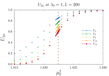
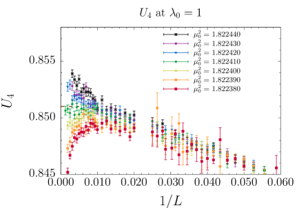
Figure 4.1: The left panel shows Binder cumulants up to twelfth order vs. $\mu_{0}^{2}$ for fixed simplicial complex size, $L=200$ and $\lambda_{0}=1$. The vertical dashed line indicates $\mu_{a}^{2}\approx\mu_{\mathrm{cr}}^{2}$. The right panel shows the cumulant $U_{4}$ vs. simplicial complex size $L$ in the pseudocritical region holding $\lambda_{0}=1$ fixed. Each point represents a calculation and connecting lines indicate constant $\mu_{0}^{2}$. Continuum estimate: $U_{4}^{*}=0.8510207(63)$.

In the left panel of Fig. 4.1, we show the cumulants for a fixed size of the simplicial complex ($L=200$) as we sweep through the critical region by varying $\mu^{2}_{0}$ holding $\lambda_{0}=1$ fixed. Higher order cumulants are statistically noisier but since they pass through the critical region with a steeper slope [35] they have comparable statistical weight in determining the critical coupling $\mu_{a}^{2}\approx\mu_{\mathrm{cr}}^{2}$. On the right we show the cumulant $U_{4}$ vs. simplicial complex size $L$ for fixed values of $\mu^{2}_{0}$ in the critical region. As expected, the divergence at large $L$ changes sign as $\mu^{2}_{0}$ passes through the critical region.

We will now proceed to describe our data fitting and analysis procedure. To estimate quantities like $U_{4}^{*}$ as accurately as possible, we use an iterative procedure to determine which ensembles, labeled by $(\mu_{0}^{2},\lambda_{0},L)$, to include in the fits to various moments of magnetization.

$w$	0.03
$\alpha_{3}$	$-22.9(4.7){\times}10^{3}$
$\alpha_{5}$	$12.4(3.3){\times}10^{10}$
$a_{20}$	0.47895(11)
$\overline{a}_{21}$	0.1873(41)
$a_{40}$	-0.39006(20)
$\overline{a}_{41}$	-0.357(12)
$a_{60}$	1.3570(11)
$\overline{a}_{61}$	1.876(71)
$\overline{b}_{21}$	-18(2106)
$\overline{b}_{41}$	-23(2629)
$\overline{b}_{61}$	115(13187)
$c_{20}$	-19.9(3.1)
$\mu^{2}_{a}$	1.82241324(70)
$\mu^{2}_{b}$	4(274)
$\chi^{2}/\mathrm{dof}$	1.001
$\mathrm{dof}$	1195

Table 2: Best fit values for the parameters described in Sec. 4.2 and Appendix B for data selection window with the ratios in Eq. (4.3) bounded by $w=0.03$.

We start by getting a rough fit to the data using some initial data selection window $\mu^{2}_{0}\in\left[\mu^{2}_{\mathrm{min}},\mu^{2}_{\mathrm{max}}\right]$ and $L\in\left[L_{\mathrm{min}},L_{\mathrm{max}}\right]$ and then form the following quantities

$$\delta a_{k1} =\left|\frac{\overline{a}_{k1}\left(\mu^{2}_{0}-\mu^{2}_{a}\right)\mathbb{L}^{d-\Delta_{\epsilon}}}{a_{k0}}\right|$$

$$\delta b_{k1} =\left|\frac{\overline{b}_{k1}\left(\mu^{2}_{0}-\mu^{2}_{b}\right)\mathbb{L}^{d-\Delta_{\omega}}}{a_{k0}}\right|$$

$$\delta c_{20} =\left|\frac{c_{20}\mathbb{L}^{2\Delta_{\sigma}-d}}{a_{20}}\right|$$

Subsequently we adjust the range of data to be fit for each moment of magnetization $m_{n}$ enforcing the data cuts: $\delta a_{k1},\;\delta b_{k1},\;\delta c_{20}\leq w$, where $w$ is the width of the window, for all $k\leq n$. It makes sense that lower moments of magnetization should have larger data selection regions since they vary more slowly in the critical region relative to the higher moments, as indicated in Fig. 4.1. We then refit the new data selection and reselect the data for the same $w$ using the new fit values and then iterate until the process converges to a stable data set for that $w$. We expect that fit parameters like $a_{k0}$ will have systematic errors of $\mathcal{O}(w^{2})$ due to higher order terms in the Taylor series expansion of the moments of the free energy which we did not include in our fit. So, we would like to take $w$ to be as small as possible but also have enough data left to adequately constrain all of the important fit parameters, particularly the $a_{k0}$.

In Fig. 4.2 we see a subset of the data selected with $w=0.03$ and curves with error bands computed from the best fit values of parameters shown in Table 2. Using the values shown in the table for $w=0.03$, we get $U_{4,cr}=0.85020(58)(90)$ and $U_{6,cr}=0.77193(37)(90)$ where the first error is statistical from the fit and the second is systematic.

In summary, the comparison of our Monte Carlo estimate on the QFE ${\mathbb{S}}^{2}$ with the exact solution are the following:

Monte Carlo Values: $$U_{4,cr}=0.85020(58)(90) U_{6,cr}=0.77193(37)(90)$$

Analytic CFT Values: $$U^{*}_{4}=0.8510207(63) U^{*}_{6}=0.7731441(213)$$ (4.23)

We see $O(10^{-3})$ agreement within the error estimates. Although even more stringent tests can be made, with the development of faster parallel code and a more extensive use of FSS analysis, we feel this is substantial support for the convergence of our QFE method to the exact $c=1/2$ minimal CFT. In the next section we give further tests for the two-point and four-point correlation functions.

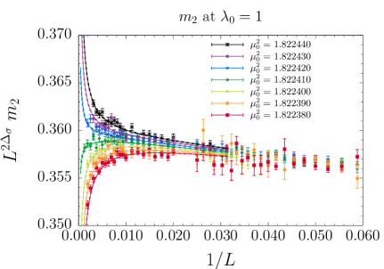
Figure 4.2: A subset of the data used in a simultaneous fit to the three lowest even moments for data selection parameter $w=0.03$.

5 Conformal Correlator on ${\mathbb{S}}^{2}$

With our results for the Binder cumulants, we are confident that the QFE lattice action on $\mathbb{S}^{2}$ has the correct critical limit. Our analysis of magnetization moments and cumulants involves global averages over n-point correlators. Here we turn to correlators to examine more closely other consequences of conformal symmetry and to provide more stringent tests for our QFE lattice action. We begin with the two-point functions $\mathbb{S}^{2}$, and explain how, with rotational invariance, the exact analytic result can best be tested against our numerical result via a Legendre expansion. We next move to the exact four-point correlator, which takes on a relatively simple form as a sum of Virasoro blocks. Finally we use this as a toy example to learn how to compute CFT data (dimensions and couplings) from the conformal block operator product expansion (OPE). In particular, we extract the central charge $c$ from the energy momentum tensor contribution to the scalar four-point function.

5.1 Two-Point Correlation Functions

In the continuum CFT on the Riemann sphere $\mathbb{S}^{2}$, the conformal two-point function, already mentioned in Eq. (4.8), is

$$g(\theta_{12})=\langle\,\phi(\hat{r}_{1})\phi(\hat{r}_{2})\rangle=\frac{1}{|\hat{r}_{1}-\hat{r}_{2}|^{2\Delta}}=\frac{1}{(2-2\cos\theta_{12})^{\Delta}}\;,$$ (5.1)

where $\hat{r}_{1},\hat{r}_{2}$ are unit vectors in the embedding space $\mathbb{R}^{3}$ defined earlier in Eq. (2.20) and $\theta_{12}$ is the angle between them. The projection of the two-point function onto Legendre functions, $P_{l}(\cos\theta_{12})$, can be computed analytically,

$$c_{l}^{\mathrm{cont}}=\int^{1}_{-1}dz\left(\frac{2}{1-z}\right)^{1/8}P_{l}(z)\implies\frac{8}{7},\;\frac{8}{105},\;\frac{24}{805},\;\frac{408}{24955},\;\frac{680}{64883},\;\frac{22440}{3049501},\cdots$$ (5.2)

integrating over $z=\cos\theta_{12}$ for $l=0,1,2,\cdots$.

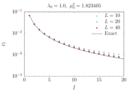
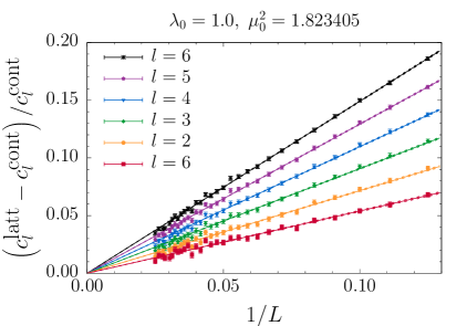
Figure 5.1: On the left, we show the simplicial two-point functions $c_{l}(L)$ projected into Legendre coefficients for various values of $L$, with the naïve dependence on $l$ scaled out for clarity of presentation. On the right, we show the relative difference between the simplicial and continuum Legendre coefficients as we take the continuum limit for fixed $l$.

In Fig. 5.1, we compare the analytic value to the moments of our correlation data. The fit is excellent showing only slight deviations at high $l$ due to cut-off effects. Our simplicial calculation of the two-point function is made at a fixed value of $\mu^{2}_{0}$ closest to the pseudocritical values $\mu_{a}^{2}$ in Table 2. In Fig. 5.1, the normalization of the simplicial Legendre coefficients $c_{l}(L)$ are chosen so that $c_{0}(L)=c_{0}^{\mathrm{cont}}=8/7$. In the left panel, we see that for any fixed value of $L$ the difference between the simplicial and continuum values is small at small $l$ but increases with increasing $l$. Yet as $L$ increases, all simplicial coefficients converge towards their continuum values. The right panel shows how the simplicial coefficients behave at fixed $l$ as we approach the continuum limit. The scaling curves shown assume a naïve $1/L$ scaling of simplicial artifacts, which turns out to be a good description of the data.

More generally in a CFT on the sphere, we will fit the two-point function to determine the operator dimension, $\Delta_{\sigma}$. This can be done directly in co-ordinate space by fitting to Eq. (5.1) up to an overall normalization, or numerically to the Legendre coefficients, $c_{l}^{\mathrm{cont}}(\Delta_{\sigma})=\int^{1}_{-1}dz\left(2/(1-z)\right)^{\Delta_{\sigma}}P_{l}(z)$, which obey the closed form recursion relation,

$$c_{l}^{\mathrm{cont}}(\Delta_{\sigma})=\frac{l-1+\Delta_{\sigma}}{l+1-\Delta_{\sigma}}\;c_{l-1}^{\mathrm{cont}}\quad,\quad c_{0}^{\mathrm{cont}}(\Delta_{\sigma})=\frac{1}{1-\Delta_{\sigma}}\;.$$ (5.3)

The overal normalization $c_{0}^{\mathrm{cont}}$ is of course proportional to $m_{2}$ defined in Eq. (4.2). With our current simulations of $\phi^{4}$ theory on ${\mathbb{S}}^{2}$, both methods agree with the exact value $\Delta_{\sigma}=0.125$ at the percent level.

From our analysis of the two-point function, we have a direct demonstration of how rotational symmetry is restored in the continuum limit. Because the two-point function can be represented as an expansion in Legendre functions, it is a function of only the angle between any two points on the sphere and therefore rotationally invariant. For any fixed finite $l$, no matter how large, the simplicial coefficient $c_{l}(L)$ converges to the continuum one as $L\to\infty$.

5.2 Four Point Functions

The $c=1/2$ minimal CFT has only three Virasoro primaries ${\bf 1},\sigma,\epsilon$, with an OPE expansion,

$$\sigma\times\sigma={\bf 1}+\epsilon\,,\quad\epsilon\times\sigma=\epsilon\,,\quad\epsilon\times\epsilon={\bf 1}\;.$$ (5.4)

In our earlier paper [19], we constructed a simplicial Wilson representation of Dirac Fermions ${\mathbb{S}}^{2}$. The map to the holomorphic, $\psi(z)$, and anti-holomorphic, $\bar{\psi}(\bar{z})$, components of free Majorana fields on all 2-d Riemann surfaces [52] allowed us to define $\epsilon=\bar{\psi}\psi$ and therefore compute the four-point functions: $\langle\,\epsilon_{1}\epsilon_{2}\epsilon_{3}\epsilon_{4}\rangle$ and $\langle\,\sigma_{1}\epsilon_{1}\sigma_{2}\epsilon_{1}\rangle$ without Monte Carlo simulations. Here we test our QFE $\phi^{4}$ construction on ${\mathbb{S}}^{2}$ to compute the $\langle\,\sigma_{1}\sigma_{2}\sigma_{3}\sigma_{4}\rangle$ correlator. In the continuum limit the leading behavior of the lattice field is the primary operator: $\phi_{x}\sim\sigma(x)+O(1/L^{\Delta_{\sigma}-\Delta^{\prime}_{\sigma}})$. The four-point function $\langle\,\phi(\hat{r}_{1})\phi(\hat{r}_{2})\phi(\hat{r}_{3})\phi(\hat{r}_{4})\rangle$ is a function invariant under any of the 24 permutations of the four positions. This permutation invariance is easily enforced even on a finite lattice. In the continuum, the eight real coordinates can be reduced to five real coordinates using rotational invariance alone.

Conformal symmetry allows for a further reduction to four real coordinates, the two angular variables $\theta_{13}$ and $\theta_{24}$ defined as in Eq. (5.1), plus two real conformal cross ratios $u$ and $v$

$$u\equiv\frac{|\hat{r}_{1}-\hat{r}_{2}|^{2}|\hat{r}_{3}-\hat{r}_{4}|^{2}}{|\hat{r}_{1}-\hat{r}_{3}|^{2}|\hat{r}_{2}-\hat{r}_{4}|^{2}}=|z|^{2},\quad v\equiv\frac{|\hat{r}_{1}-\hat{r}_{4}|^{2}|\hat{r}_{3}-\hat{r}_{2}|^{2}}{|\hat{r}_{1}-\hat{r}_{3}|^{2}|\hat{r}_{2}-\hat{r}_{4}|^{2}}=|1-z|^{2}\;,$$ (5.5)

or equivalently a single complex variable $z$.

$$z=\frac{(w_{1}-w_{2})(w_{3}-w_{4})}{(w_{1}-w_{3})(w_{2}-w_{4})}\quad\implies\quad 1-z=\frac{(w_{2}-w_{3})(w_{1}-w_{4})}{(w_{1}-w_{3})(w_{2}-w_{4})}$$ (5.6)

where $w$ is the complex variable for the ${\mathbb{R}}^{2}$ prior to the stereographic project to ${\mathbb{S}}^{2}$ in Eq. (4.6). In these variables, the four-point function can be written

$$G(z)=\frac{\left\langle\phi_{1}\phi_{2}\phi_{3}\phi_{4}\right\rangle}{\left\langle\phi_{1}\phi_{3}\right\rangle\ \left\langle\phi_{2}\phi_{4}\right\rangle}\;.$$ (5.7)

where the dependence on $\theta_{13}$ and $\theta_{24}$ cancels in the ratio. While $G(z)$ has the exchange symmetries in the t-channel ($1\leftrightarrow 3$, $2\leftrightarrow 4$), combining this properly with the Möbius map $z\rightarrow 1-z,z\rightarrow 1/z$ gives 24 copies, transforming the blue fundamental zone on the left-hand side of Fig. 5.2 to the entire complex z plane. In the specific case of the $c=1/2$ minimal model, the explicit form of $G(z)$ is known in polar coordinates $z=re^{i\theta}$ as

$$G(u,v)=v^{\Delta}g(u,v) = \frac{1}{2|z|^{1/4}|1-z|^{1/4}}\left[|1+\sqrt{1-z}|+|1-\sqrt{1-z}|\right]$$ (5.8)

$$= \frac{1}{2|z|^{1/4}|1-z|^{1/4}}\sqrt{2+2\sqrt{(1-z)(1-\bar{z})}+2\sqrt{z\bar{z}}}\;.$$

The first form is a sum of the two Virasoro blocks and the second form, given in Ref. [36], is the explicitly crossing symmetric form. For visualization, we plot $G(z)$ in Fig. 5.2.

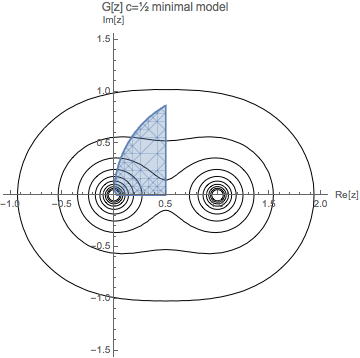
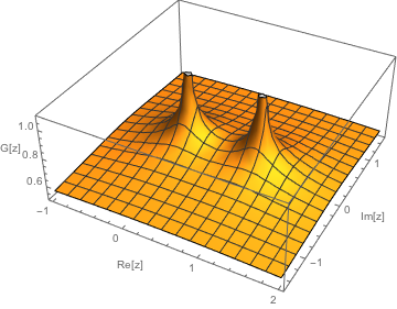
Figure 5.2: We visualize the conformal function $G(z)$ in contour and surface renderings. The outermost contour starts at $G(z)=0.6$ and increases by steps of 0.1. Two symmetry planes are apparent: Re($z$)=1/2 and Im($z$)=0. These are related to certain permutations of the four-point function. The entire set of permeations maps the blue zone exactly to the entire complex plane.

Given that independent field configurations on our simplicial complexes can be generated in nearly $\mathcal{O}(L^{2})$ time, the dominant cost of computing the four-point function would naïvely be computing the product of four fields which scales as $\mathcal{O}(L^{8})$ and would be intractable for large $L$ close to the continuum limit. We can reduce the cost by only sampling a subset of values of the four-point function on each independent configuration we generate. This is achieved by drawing $\mathcal{O}(L^{2})$ quartets of random points on the simplicial complex. This balances the computational cost equally between generating independent field configurations and sampling the four-point function.

We then determine the product of the four simplicial fields, the unique coordinates $(\theta_{13},\theta_{24},z)$ under the permutations of the positions, and finally an estimate of $G(z)$ by dividing our product of simplicial fields by the continuum two-point function, Eq. (4.8), which is justified by our success of the previous section in showing that the simplicial two-point function converges correctly in the continuum limit,

$$G(z)=\frac{\left\langle\phi_{1}\phi_{2}\phi_{3}\phi_{4}\right\rangle}{g(\theta_{13})g(\theta_{24})}\to\frac{\left\langle\phi_{1}\phi_{2}\phi_{3}\phi_{4}\right\rangle}{\left\langle\phi_{1}\phi_{3}\right\rangle\left\langle\phi_{2}\phi_{4}\right\rangle}\quad\mathrm{as}\quad L\to\infty\;.$$ (5.9)

For convenience when studying the four-point function, we bin the data by coordinate on the complex plane. We partition the unit disk $|z|\leq 1$ on the complex plane into a radial grid of $N^{2}_{0}$ bins of equal area. The angular width of each bin is $\Delta\theta=2\pi/N_{0}$ and we choose $N_{0}\bmod 4=0$ so that the bins are centered at $\theta_{n}=0,\pi/2,\pi,3\pi/2$. This arrangement is ideal for using standard discrete cosine transforms (DCT-I) for computing Fourier coefficients. For this study we chose $N_{0}=64$.

We present a subset of our results for the conformal portion of the four-point function, Eq. (5.8), in Fig. 5.3. Here, we consider the fixed slice $r\in[0,1]$ for $\theta=0$. We see that, even for moderately small values of $L$, the measured four-point function converges well to the analytic, continuum result.

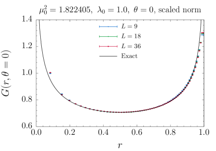
Figure 5.3: Results for the conformal part of the QFE scalar four-point function of the Ising universality class on $\mathbb{S}^{2}$. $G(r,\theta)$ should only depend on a single complex coordinate $z=re^{i\theta}$. We have computed the four-point function in the entire complex plane in $\phi^{4}$ theory and show the function for $r\in[0,1]$ at fixed $\theta=0$ as it converges to the continuum result.

5.3 Operator Product Expansion

In Sec. 5.2, we calculated the simplicial approximation to the scalar four-point function which, after taking a ratio with a product of two-point functions respecting $t$-channel symmetry, is described by a conformal function $G(z)$ invariant under $z\to 1-z$ and $z\to\bar{z}$. We computed the function everywhere in the unit circle, which can then be extended to the whole complex plane utilizing the permutation symmetry of the full four-point function. Our representation of the function $G(z)$ is a tabulation of values on an equal area grid in polar coordinates $(r,\theta)$.

In the conformal bootstrap the expansion around $z=0$ is used based on the operator product expansion (OPE). It is interesting to ask how well our Monte Carlo simulation on ${\mathbb{S}}^{2}$ can determine the data in an OPE expansion,

$$G_{s}(z)=\frac{\left\langle\phi_{1}\phi_{2}\phi_{3}\phi_{4}\right\rangle}{g(\theta_{12})g(\theta_{34})}=|z|^{\Delta_{\sigma}}G(z)=\sum_{\Delta_{\mathcal{O}},l}\lambda_{\mathcal{O}}^{2}g_{\Delta_{\mathcal{O}},l}(z)\;,$$ (5.10)

where $G_{s}(z)$ is $s$-channel symmetric, i.e. symmetric under interchange $1\leftrightarrow 2$ and $3\leftrightarrow 4$, $\Delta_{\mathcal{O}}$ are the scaling dimensions of conformal primary operators $\mathcal{O}$, and $l$ labels the spin. The functions $g_{\Delta_{\mathcal{O}},l}(z)$ are called conformal blocks whose functional form is completely determined by conformal symmetry. In $d=2$, there is an explicit representation of the conformal blocks in terms of hypergeometric functions,

$$g_{\Delta,l}(z) = \frac{1}{2}\left[z^{h}\,{}_{2}F_{1}(h,h;2h;z)\right]\left[{\bar{z}}^{\bar{h}}\,{}_{2}F_{1}(\bar{h},\bar{h};2\bar{h};\bar{z})\right]\;,$$

$$h=\frac{\Delta+l}{2},\quad\bar{h}=\frac{\Delta-l}{2}\;.$$

The expansion in Fourier modes is given by

$$g_{\Delta,l}(r,\theta)=\sum_{m=0}^{\infty}\cos(m\theta)\left[r^{\Delta}\sum_{|n-n^{\prime}+l|=m}\frac{(h)_{n}^{2}(\bar{h})_{n^{\prime}}^{2}}{(2h)_{n}(2\bar{h})_{n^{\prime}}}\frac{r^{n+n^{\prime}}}{n!{n^{\prime}}!}\right]\;,$$ (5.12)

using the Pochhammer symbol $(a)_{n}=\Gamma(a+n)/\Gamma(a)$.

With a conserved energy momentum tensor $T$, there are special terms in the OPE expansion of the scalar four-point function which have integer powers: $1+\lambda_{T}^{2}\,g_{T,2}(r,\theta)$. The identity operator term is normalized to unity by convention. The conformal block for the energy momentum tensor has a closed form expression,

$$g_{T,2}(z) = -3\left(1+\frac{1}{z}\left(1-\frac{z}{2}\right)\log(1-z)\right)\,+\,\mathrm{c.c.}$$

$$= \frac{1}{2}r^{2}\cos(2\theta)+\frac{1}{2}r^{3}\cos(3\theta)+\frac{9}{20}r^{4}\cos(4\theta)+\cdots\;,$$

and the OPE coefficient $\lambda_{T}^{2}$ is related to the central charge of the CFT,

$$\lambda_{T}^{2}=\frac{\Delta_{\sigma}^{2}d^{2}}{C_{T}(d-1)^{2}}\to\frac{1}{16C_{T}}\,\mbox{\quad\quad for~{}}\,d=2\;,$$ (5.14)

where $C_{T}=2c=2(1/2)=1$ for the $d=2,c=1/2$ minimal model.

We can extract an estimate of the central charge $c$ from our simplicial calculation of the scalar four-point function by modeling the result with the first few terms in the OPE expansion

$$G_{s}(r,\theta)\propto 1+\lambda_{\epsilon}^{2}\,g_{\epsilon,0}(r,\theta)+\lambda_{T}^{2}\,g_{T,2}(r,\theta)$$ (5.15)

We used a DCT-I to Fourier transform the data, simultaneously fitting $m=0,2$ to four parameters: the overall normalization, $\lambda_{\epsilon}^{2}$, $\lambda_{T}^{2}$ and $\Delta_{\epsilon}$. We choose a single value of $\mu^{2}=1.822410$ which is close to the pseudocritical value, and we restrict the fitting range in $r$ around 0.5 where the data shows the least discretization error. A fit for $L=36$ and $0.25\leq r\leq 0.75$ is shown in Fig. 5.4. A summary of several fits is shown in Table 3. As expected, the fit values converge towards the continuum CFT results $(\Delta_{\epsilon}=1,\lambda_{\epsilon}^{2}=1/4,c=1/2)$ as $L$ increases towards the continuum limit and as the fit range in $r$ is confined to a narrower region around $r=0.5$ where the discretization artifacts appear smallest.

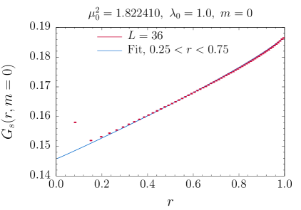
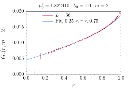
Figure 5.4: On the left, a fit to the $m=0$ Fourier component of the $s$-channel symmetric conformal part of the four-point function. On the right, a fit to the $m=2$ Fourier component. A simultaneous fit to both components can be used to fix the normalization of the four-point function and determine the central charge.

$\mu^{2}$	$s$	$r_{\mathrm{min}}\leq r\leq r_{\mathrm{max}}$	norm	$\Delta_{\epsilon}$	$\lambda_{\epsilon}^{2}$	$c$
1.82241	9	$0.25\leq r\leq 0.75$	0.2900	1.075	0.2536	0.4668
1.82241	9	$0.30\leq r\leq 0.70$	0.2901	1.075	0.2533	0.4704
1.82241	9	$0.35\leq r\leq 0.65$	0.2902	1.077	0.2533	0.4738
1.82241	9	$0.40\leq r\leq 0.60$	0.2902	1.016	0.2427	0.4747
1.82241	18	$0.25\leq r\leq 0.75$	0.2051	1.068	0.2563	0.4866
1.82241	18	$0.30\leq r\leq 0.70$	0.2051	1.056	0.2544	0.4878
1.82241	18	$0.35\leq r\leq 0.65$	0.2051	1.050	0.2535	0.4904
1.82241	18	$0.40\leq r\leq 0.60$	0.2051	1.046	0.2526	0.4884
1.82241	36	$0.25\leq r\leq 0.75$	0.1457	1.031	0.2528	0.4926
1.82241	36	$0.30\leq r\leq 0.70$	0.1458	1.026	0.2519	0.4932
1.82241	36	$0.35\leq r\leq 0.65$	0.1458	1.018	0.2508	0.4931
1.82241	36	$0.40\leq r\leq 0.60$	0.1458	1.007	0.2486	0.4933

Table 3: A summary of several fits to the $m=0,1,2,3$ Fourier components of the $s$-channel symmetric conformal part of the four-point function.

int

6 Conclusion

We have set up the basic formalism for defining a scalar field theory on non-trivial Riemann manifolds and tested it numerically in the limited context of the 2-d $\phi^{4}$ theory by comparing it against the $c=1/2$ Ising CFT at the Wilson-Fisher fixed point. This test is at a sufficient accuracy compared with the exact result to encourage us that we are able to define this strongly coupled quantum field theory on a curved manifold, in this case ${\mathbb{S}}^{2}$. Faster parallel code could push these tests to much higher precision. While this may be pursued in future works, our goal here was to sketch a framework for lattice quantum field theories on a non-trivial Riemann manifold as a quantum extension of FEM which we refer to as Quantum Finite Elements (QFE). Whether or not this has generally applicability remains, of course, to be proven.

Our construction first relies on theoretical issues in the application of FEM that, in spite of the vast literature, are not to our knowledge proven in enough generality. Nonetheless, the documented experience with FEM for PDEs does argue that this framework likely extends when properly formulated to convergence to the classical limit of any renormalizable quantum field theory on a smooth Euclidean Riemann manifold [19]. A rather non-trivial extension of the classical finite element/DEC method for the lattice Dirac Fermion and non-Abelian gauge fields on a simplicial Riemannian manifold is provided in Ref. [19] and Ref. [22] respectively. The local spin and gauge invariance on each site is achieved by compact spin connections and compact gauge links. This we believe provides the basic tools for classical simplicial constructions.

Second, and most importantly, we show that reaching the continuum for a quantum FEM Lagrangian requires a modification of the action by counter terms to accommodate UV effects. We conjecture that for a super-renormalizable theory with a finite number of divergent diagrams, a new QFE lattice action can be constructed by a natural generalization of $\phi^{4}$ theory example presented here that removes the scheme dependence of the FEM simplicial lattice UV cut-off. The detailed generalization of this conjecture needs to be investigated with many more examples and most likely alternative approaches.

Third, once we have successfully constructed the QFE action with UV counter terms consistent with the continuum limit to all orders in perturbation theory, we conjecture that it represents a correct formulation of the non-perturbative quantum field theory on a curved Riemann manifold. This parallels the conventional wisdom for LFTs on hypercubic lattices that when lattice symmetries are protected (Lorentz, chiral, SUSY) only a finite set of fine tuning parameters are need to reach the continuum theory. Further research is need to establish the range of applicability of our QFE proposal. More examples are obviously need to support this proposal.

There are many more direct extensions of this formulation that we are currently entertaining. The first is to apply QFE to the 3-d $\phi^{4}$ theory in both radial quantization and the 3-d projective sphere, ${\mathbb{S}}^{3}$. Our current software relies on a serial code and the very efficient Brower-Tamayo [32] modification of the cluster algorithm. We are in the process of developing parallel code that will allow for large lattices and higher precision, which will also be a necessity in going beyond 2d and scalar fields. Although new software requires substantial effort, we believe that all of the fundamental data parallel concepts and advanced algorithms utilized in lattice QCD will still be applicable here. We note there are advantages to studying CFTs on spherical ${\mathbb{S}}^{d}$ simplicial lattices. There are no finite volume approximations. The entire ${\mathbb{R}}^{d}$ is mapped to the sphere. For radial quantization the only finite volume effect is the one radial dimension along the ${\mathbb{R}}\times{\mathbb{S}}^{d-1}$ cylinder. With periodic boundary conditions, the finite extent of the cylinder is also an interesting parameter for the study of CFTs at finite temperature. Radial quantization on ${\mathbb{R}}\times{\mathbb{S}}^{d-1}$ allows direct access to the Dilatation operator to compute operator dimensions and the OPE expansion. Even our 2-d example is worth further investigation at higher precision, and with an emphasis on new studies enabled by a fully non-perturbative formulation of the $\phi^{4}$ theory on ${\mathbb{S}}^{2}$. For example, we can consider new ways to compute the renormalization flow of the central charge from the UV to the IR. Further research is on going to hopefully justify this optimism.

Appendix A Free Theory on Sphere and Cylinder

Here we collect a few analytic expressions for the free scalar theory that are useful in establishing convergence of the simplicial propagators to the exact continuum on the ${\mathbb{S}}^{2}$ and ${\mathbb{R}}\times{\mathbb{S}}^{2}$ manifolds.

Free scalar on a sphere:

The Green’s function on the sphere is given by spectral sum,

$$G(\theta,\mu)=\sum^{\infty}_{l=0}\sum^{l}_{m=-l}\frac{Y^{*}_{lm}(\hat{r}_{1})Y_{lm}(\hat{r}_{2})}{l(l+1)+1/4+\mu^{2}}=\frac{1}{4\pi}\sum^{\infty}_{l=0}\frac{(2l+1)P_{l}(cos\theta)}{(l+1/2)^{2}+\mu^{2}}\,,$$ (A.1)

where $\hat{r}_{1}\cdot\hat{r}_{2}=\cos(\theta_{12})=z$. For generality we have added a dimensionless “mass” term $m^{2}_{0}=\mu^{2}+1/4$ to regulate the IR. The series can also be summed to get

$$G(\theta,\mu)=\frac{1}{4\pi}[Q_{-1/2+i\mu}(z)+Q_{-1/2-i\mu}(z)]\;.$$ (A.2)

in term of associated Legendre functions. This Green’s function (A.2) can also be written in compact integral representation,

$$G(\theta,\mu)=\frac{1}{4\pi}\int^{\infty}_{-\infty}dte^{\textstyle i\mu t}G(t,\theta)=\frac{1}{2\pi}\int^{\infty}_{0}\frac{\cos(\mu t)dt}{\sqrt{2\cosh(t)-2\cos(\theta)}}\;,$$ (A.3)

exhibiting clearly the logarithmic singularity as $1-z\rightarrow\theta^{2}/2$. Expanding the integral we find,

$$G(\theta,\mu)\simeq\frac{1}{4\pi}[\log[\frac{32}{1-\cos(\theta)}]-14\zeta(3)\mu^{2}]+O(\theta^{2},\mu^{4})\;,$$ (A.4)

in agreement with Eq. (3.24) in Sec. 3.3.

Conformal propagator on a cylinder:

Next, we consider the 3-d conformal propagator for radial quantization on ${\mathbb{R}}\times{\mathbb{S}}^{2}$,

$$G(t,\theta) = \langle\,\phi(x_{1})\phi(x_{2})\rangle=(r_{1}r_{2})^{\Delta}\frac{1}{|x_{1}-x_{2}|^{2\Delta}}$$ (A.5)

$$= \frac{1}{[r_{1}/r_{2}+r_{2}/r_{1}-2\cos(\theta)]^{\Delta}}=\frac{1}{[2\cosh(t)-2\cos(\theta)]^{\Delta}}\;,$$

where $t=t_{2}-t_{1}=\log(r_{2}/r_{1})$. Note by setting $t=0$, this is exactly the conformal two point function on the sphere Eq. (4.8) as expected by dimensional reduction. (In the rest of the appendix, we also drop the factor of $1/(4\pi)$ to coincide with the normalization convention in Sec. 5.)

However, if we return to the 3-d free theory, setting $\Delta=(d-2)/2=1/2,$ the dimensional reduction by setting $t=0$ in the 3-d conformal propagator fails to give the 2-d propagator. To understand this we recall that in 2d, the scalar field, $\phi(x)$ is not a primary operator. As is well known in string theory, conformal primaries are given by vertex operators $:\exp[ik\phi]:$. Instead, to reach the free Green’s function from the cylinder, we proceed as follows. The multipole expansion of the Coulomb term is

$$\frac{1}{|x_{1}-x_{2}|}=\frac{1}{\sqrt{r_{1}r_{2}}}\sum_{l}(r_{1}/r_{2})^{l+1/2}P_{l}(\cos\theta)$$ (A.6)

for $r_{2}>r_{1}$ or $r_{2}>r_{1}$ , after interchanging $r_{1}$ and $r_{2}$. Thus the Green’s function is

$$G(t,\theta)=\sum_{l}[\theta(t)e^{\textstyle-(l+1/2)t}+\theta(-t)e^{\textstyle(l+1/2)t}]P_{l}(\cos\theta)$$ (A.7)

rescaling by $\sqrt{r_{1}r_{2}}$ as in Eq. (A.5) above. In Fourier space this becomes

$$\widetilde{G}(\omega,\theta)=\int^{\infty}_{-\infty}dte^{\textstyle i\omega t}G(t,\theta) = \int^{\infty}_{0}dte^{\textstyle i\omega t}\sum_{l}e^{\textstyle-(l+1/2)t}P_{l}(\cos\theta)$$ (A.8)

$$+ \int^{0}_{-\infty}dte^{\textstyle i\omega t}\sum_{l}e^{\textstyle(l+1/2)t}P_{l}(\cos\theta)\;,$$

so

$$\widetilde{G}(\omega,\theta) = \sum^{\infty}_{l=0}[\frac{1}{l+1/2+i\omega}+\frac{1}{l+1/2-i\omega}]P_{l}(\cos\theta)$$ (A.9)

$$= \sum_{l}\frac{(2l+1)P_{l}(\cos\theta)}{(l+1/2)^{2}+\omega^{2}}\;.$$

By fixing the frequency $\omega^{2}=\mu^{2}$ we regain the free propagator on the sphere. We take the value $\mu=0$ as our standard IR regulated propagator which has an appealing interpretation as constant line source in 3d. Of course in practice on the lattice for our 3-d simulations, we will introduce a finite cylinder of length $T=aL_{t}$, with periodic boundary conditions. This corresponds to the thermal propagators, with periodic $t\in[0,T]$ represented by a discrete sum,

$$G(t,\theta)=\int\frac{d\omega}{2\pi}e^{\textstyle-i\omega t}\widetilde{G}(\omega,\theta)\rightarrow\frac{1}{T}\sum_{n}e^{\textstyle-i\omega_{n}t}\widetilde{G}(\omega_{n},\theta)$$ (A.10)

over frequencies, $\omega_{n}=2\pi n/T$.

Appendix B Finite Size Scaling for Cumulants and Moments

This follows the renormalization group arguments first presented in [44] and reviewed in [51]. We begin with the free energy Eq. (4.4),

$$\mathcal{F}\left(g_{\sigma},g_{\epsilon},\{g_{\omega},\dots\},a\right)=\log Z\quad,\quad Z=\int\left[D\phi\right]\;e^{\textstyle-S+h\int d^{d}x\phi(x)}\;$$ (B.1)

expressed not as a function of the bare couplings $h,\mu^{2}_{0},\lambda_{0}$ but rather the relevant couplings $g_{\sigma},g_{\lambda}$ and the irrelevant couplings $\left\{g_{\omega},\dots\right\}$ of the Wilson-Fisher fixed point. For the lattice spacing, we assume $a\sim 1/L$. Under a change of scale by a factor $l$, the free energy renormalizes

$$\mathcal{F}\left(g_{\sigma},g_{\epsilon},\{g_{\omega},\dots\},a\right)=l^{-d}F\left(l^{y_{\sigma}}g_{\sigma},l^{y_{\epsilon}}g_{\epsilon},\{l^{y_{\omega}}g_{\omega},\dots\},la\right)+G\left(g_{\sigma},g_{\epsilon}\right)$$ (B.2)

where $y_{\mathcal{O}}\equiv d-\Delta_{\mathcal{O}}$, $F$ is the singular, or scaling, part of the free energy and $G$ is the regular part. In what follows, we will continue to use $y_{\mathcal{O}}$ instead of $\Delta_{\mathcal{O}}$ for compactness of notation.

If we choose ${\mathbb{L}}\equiv\sqrt[d]{\Omega_{d}}$, where $\Omega_{d}$ is the volume of the $d$-dimensional manifold, and differentiate the free energy $k$ times with respect to $g_{\sigma}$ and then take the limit $g_{\sigma}\to 0$ we get

$$\frac{\partial^{k}\mathcal{F}}{\partial g_{\sigma}^{k}}=\mathcal{F}^{(k)}\left(g_{\epsilon},\{g_{\omega},\dots\},1/{\mathbb{L}}\right)={\mathbb{L}}^{ky_{\sigma}-d}F^{(k)}\left({\mathbb{L}}^{y_{\epsilon}}g_{\epsilon},\{{\mathbb{L}}^{y_{\omega}}g_{\omega},\dots\},1\right)+G^{(k)}(g_{\epsilon})\;.$$ (B.3)

We compute derivatives of the free energy with respect to the bare parameter $h$ and then take the limit $h\to 0$, to get cumulants of the magnetization

$$\kappa_{k}=\lim_{h\to 0}\frac{1}{\Omega_{d}^{k-1}}\frac{\partial^{k}\mathcal{F}}{\partial h^{k}}\;,$$ (B.4)

and put them in the form of Binder cumulants,

$$U_{2n}\propto\lim_{h\to 0}\frac{\kappa_{2n}}{\kappa_{2}^{n}}\;,$$ (B.5)

with the normalization to be determined as described in Sec. 4.1. We note that the symmetry $\phi\to-\phi$ guarantees that all odd cumulants vanish, $\kappa_{2n+1}=0$ and that $h$ is an odd-function of $g_{\sigma}$. To take advantage of the RG scaling properties of the free energy near the critical point, we must rewrite the cumulants carefully using the chain rule. To make the following manageable, we define $\alpha_{2n+1}$ and understand that all expressions are in the limit $g_{\sigma},h\to 0$,

$$\alpha_{2n+1} \equiv \lim_{h\to 0}\frac{\partial^{2n+1}g_{\sigma}}{\partial h^{2n+1}}\;,$$ (B.6)

$${\mathbb{L}}^{2\Delta_{\sigma}}\kappa_{2} = \alpha_{1}^{2}\left[F^{(2)}+{\mathbb{L}}^{-d+2\Delta_{\sigma}}G^{(2)}\right]\;,$$ (B.7)

$${\mathbb{L}}^{4\Delta_{\sigma}}\kappa_{4} = \alpha_{1}^{4}\left[F^{(4)}+{\mathbb{L}}^{-3d+4\Delta_{\sigma}}G^{(4)}\right]+\alpha_{1}\alpha_{3}\left[{\mathbb{L}}^{-2d+2\Delta_{\sigma}}F^{(2)}+{\mathbb{L}}^{-3d+4\Delta_{\sigma}}G^{(2)}\right]\;,$$ (B.8)

$${\mathbb{L}}^{6\Delta_{\sigma}}\kappa_{6} = \alpha_{1}^{6}\left[F^{(6)}+{\mathbb{L}}^{-5d+6\Delta_{\sigma}}G^{(6)}\right]+\alpha_{1}^{3}\alpha_{3}\left[{\mathbb{L}}^{-2d+2\Delta_{\sigma}}F^{(4)}+{\mathbb{L}}^{-5d+6\Delta_{\sigma}}G^{(4)}\right]$$ (B.9)

$$+(\alpha_{3}^{2}+3\alpha_{1}\alpha_{5})\left[{\mathbb{L}}^{-4d+4\Delta_{\sigma}}F^{(2)}+{\mathbb{L}}^{-5d+6\Delta_{\sigma}}G^{(2)}\right]$$

$${\mathbb{L}}^{8\Delta_{\sigma}}\kappa_{8} = \alpha_{1}^{8}\left[F^{(8)}+{\mathbb{L}}^{-7d+8\Delta_{\sigma}}G^{(8)}\right]+56\alpha_{1}^{5}\alpha_{3}\left[{\mathbb{L}}^{-2d+2\Delta_{\sigma}}F^{(6)}+{\mathbb{L}}^{-7d+8\Delta_{\sigma}}G^{(6)}\right]\;,$$ (B.10)

$$+(280\alpha_{1}^{2}\alpha_{3}^{2}+56\alpha_{1}^{3}\alpha_{5})\left[{\mathbb{L}}^{-4d+4\Delta_{\sigma}}F^{(4)}+{\mathbb{L}}^{-7d+8\Delta_{\sigma}}G^{(4)}\right]$$

$$+(56\alpha_{3}\alpha_{5}+8\alpha_{1}\alpha_{7})\left[{\mathbb{L}}^{-6d+6\Delta_{\sigma}}F^{(2)}+{\mathbb{L}}^{-7d+8\Delta_{\sigma}}G^{(2)}\right]\;$$

At this point, the pattern is clear and the only difficulty extending the calculation to higher cumulants is computing the associated chain rule factors which are relatively straight-forward to compute using a program like Mathematica. For example, D[f[g[h]],{h,8}] will give all the terms needed for $\partial^{8}\mathcal{F}/\partial h^{8}$, remembering to set to zero odd derivatives of $\mathcal{F}$ and even derivatives of $g$.

Before we continue, we point out an important physical concept. At finite ${\mathbb{L}}$, the difference between the lattice scalar operator $\phi$ and the conformal primary operator $\sigma$ is indicated by the presence of higher derivative terms $\alpha_{2n+1}$ in the cumulant expressions. But, in the scaling limit ${\mathbb{L}}\to\infty$ all those terms vanish and the cumulants are dominated by the moments of the free energy with respect to the coupling $g_{\sigma}$ of the conformal primary operator $\sigma$. In this sense, the simplicial operator $\phi(x)$ becomes the primary operator $\sigma(x)$ in the scaling limit.

We can now apply the important physical principle that close to the critical point we can expand the derivatives of the free energy in a Taylor series

$$F^{(k)} = a_{k0}+a_{k1}\left(g_{\epsilon}-g_{\epsilon}^{*}\right){\mathbb{L}}^{y_{\epsilon}}+\cdots+b_{k1}\left(g_{\omega}-g_{\omega}^{*}\right){\mathbb{L}}^{y_{\omega}}+\cdots.$$ (B.11)

$$G^{(k)} = c_{k0}+c_{k1}\left(g_{\epsilon}-g_{\epsilon}^{*}\right)+\cdots$$ (B.12)

Substituting these expressions into those for the cumulants defined in Eqns. (B.7) to (B.10) nearly gives us an expression we can fit to computed data. Of course, we cannot directly vary the renormalized couplings $(g_{\sigma},g_{\epsilon},g_{\omega},\cdots)$ but instead can vary our bare couplings $(h,\mu^{2}_{0},\lambda_{0})$ defined in our cutoff theory. Near the Wilson-Fisher fixed point we can relate the two sets of couplings by expanding

$$\left(\begin{array}[]{c}g_{\epsilon}-g_{\epsilon}^{*}\\ g_{\omega}-g_{\omega}^{*}\end{array}\right) = \left(\begin{array}[]{cc}R_{\epsilon\mu}&R_{\epsilon\lambda}\\ R_{\omega\mu}&R_{\omega\lambda}\end{array}\right)\left(\begin{array}[]{c}\mu^{2}_{0}-\mu_{*}^{2}\\ \lambda_{0}-\lambda_{*}\end{array}\right)+\cdots$$ (B.19)

So, substituting Eq. (4.18) first into Eqns. (B.11) to (B.12) leads to expressions that can be used to model cumulant data computed in a cutoff theory close to the Wilson-Fisher fixed point.

Often it is more convenient in the cutoff theory to compute moments instead of cumulants. The expansion of moments in terms of cumulants is well known so we only write the first few even moments here

$$m_{2} = \kappa_{2}$$ (B.20)

$$m_{4} = \kappa_{4}+3\kappa_{2}^{2}$$ (B.21)

$$m_{6} = \kappa_{6}+15\kappa_{4}\kappa_{2}+15\kappa_{2}^{3}$$ (B.22)

$$m_{8} = \kappa_{8}+28\kappa_{6}\kappa_{2}+35\kappa_{4}^{2}+210\kappa_{4}\kappa_{2}^{2}+105\kappa_{2}^{4}$$ (B.23)

$$m_{10} = \kappa_{10}+45\kappa_{8}\kappa_{2}+210\kappa_{6}\kappa_{4}+630\kappa_{6}\kappa_{2}^{2}+1575\kappa_{4}^{2}\kappa_{2}+3150\kappa_{4}\kappa_{2}^{3}+945\kappa_{2}^{5}$$ (B.24)

$$m_{12} = \kappa_{12}+66\kappa_{10}\kappa_{2}+495\kappa_{8}\kappa_{4}+1485\kappa_{8}\kappa_{2}^{2}+462\kappa_{6}^{2}+13860\kappa_{6}\kappa_{4}\kappa_{2}$$ (B.25)

$$+13860\kappa_{6}\kappa_{2}^{3}+5775\kappa_{4}^{3}+51975\kappa_{4}^{2}\kappa_{2}^{2}+51975\kappa_{4}\kappa_{2}^{4}+10395\kappa_{2}^{6}\;.$$

References

- [1] Thomas Appelquist, Richard Brower, Simon Catterall, George Fleming, Joel Giedt, Anna Hasenfratz, Julius Kuti, Ethan Neil, and David Schaich. Lattice Gauge Theories at the Energy Frontier. In Community Summer Study 2013: Snowmass on the Mississippi (CSS2013) Minneapolis, MN, USA, July 29-August 6, 2013, 2013.
- [2] R.C. Brower, G.T. Fleming, and H. Neuberger. Lattice Radial Quantization: 3D Ising. Phys.Lett., B721:299–305, 2013.
- [3] Richard Brower, Claudio Rebbi, and David Schaich. Hybrid Monte Carlo simulation on the graphene hexagonal lattice. PoS, LATTICE2011:056, 2011.
- [4] Thomas Appelquist, Richard C. Brower, George T. Fleming, Anna Hasenfratz, Xiao-Yong Jin, Joe Kiskis, Ethan T. Neil, James C. Osborn, Claudio Rebbi, Enrico Rinaldi, David Schaich, Pavlos Vranas, Evan Weinberg, and Oliver Witzel. Strongly interacting dynamics and the search for new physics at the LHC. Phys. Rev., D93(11):114514, 2016.
- [5] Julius Kuti. The Higgs particle and the lattice. PoS, KMI2013:002, 2015.
- [6] M. Luscher. Dimensional Regularization in the Presence of Large Background Fields. Annals Phys., 142:359, 1982.
- [7] I. Jack and H. Osborn. Background Field Calculations in Curved Space-time. 1. General Formalism and Application to Scalar Fields. Nucl. Phys., B234:331–364, 1984.
- [8] I. Jack and H. Osborn. General Background Field Calculations With Fermion Fields. Nucl. Phys., B249:472–506, 1985.
- [9] I. L. Buchbinder, S. D. Odintsov, and I. L. Shapiro. Renormalization Group Approach to Quantum Field Theory in Curved Space-time. Riv. Nuovo Cim., 12N10:1–112, 1989.
- [10] Richard C. Brower, George T. Fleming, and Herbert Neuberger. Radial Quantization for Conformal Field Theories on the Lattice. PoS, LATTICE2012:061, 2012.
- [11] Richard C. Brower, Michael Cheng, and George T. Fleming. Improved Lattice Radial Quantization. PoS, LATTICE2013:335, 2014.
- [12] T. Regge. GENERAL RELATIVITY WITHOUT COORDINATES. Nuovo Cim., 19:558–571, 1961.
- [13] Gilbert Strang and George Fix. An Analysis of the Finite Element Method 2nd Edition. Wellesley-Cambridge, 2nd edition, 5 2008.
- [14] M. Desbrun, A. N. Hirani, M. Leok, and J. E. Marsden. Discrete Exterior Calculus. ArXiv Mathematics e-prints, August 2005.
- [15] Douglas N. Arnold, Richard S. Falk, and Ragnar Winther. Finite element exterior calculus, homological techniques, and applications. Acta Numerica, 15:1, may 2006.
- [16] Warner A. Miller, Jonathan R. McDonald, Paul M. Alsing, David Gu, and Shing-Tung Yau. Simplicial Ricci Flow. Commun. Math. Phys., 329:579–608, 2014.
- [17] Keenan Crane. Discrete Differential Geometry: An Applied Introduction. 2018.
- [18] Slava Rychkov. EPFL Lectures on Conformal Field Theory in Dimensions. 2016.
- [19] Richard C. Brower, Evan S. Weinberg, George T. Fleming, Andrew D. Gasbarro, Timothy G. Raben, and Chung-I Tan. Lattice Dirac Fermions on a Simplicial Riemannian Manifold. Phys. Rev., D95(11):114510, 2017.
- [20] E.H. Spanier. Algebraic Topology. Springer New York, 2012.
- [21] N. H. Christ, R. Friedberg, and T. D. Lee. Weights of Links and Plaquettes in a Random Lattice. Nucl. Phys., B210:337, 1982.
- [22] N. H. Christ, R. Friedberg, and T. D. Lee. GAUGE THEORY ON A RANDOM LATTICE. Nucl. Phys., B210:310, 1982.
- [23] N.H. Christ, R. Friedberg, and T.D. Lee. Random Lattice Field Theory: General Formulation. Nucl.Phys., B202:89, 1982.
- [24] Mamdouh S. Mohamed, Anil N. Hirani, and Ravi Samtaney. Numerical convergence of discrete exterior calculus on arbitrary surface meshes, 2018.
- [25] Sean M. Carroll. Lecture notes on general relativity. 1997.
- [26] Samik Sen, Siddhartha Sen, James C. Sexton, and David H. Adams. A Geometric discretization scheme applied to the Abelian Chern-Simons theory. Phys. Rev., E61:3174–3185, 2000.
- [27] Boris N. Delaunay. Sur la sphère vide. A la mémoire de Georges Voronoï. Bull. Acad. Sci. URSS, VII Ser., 1934:793–800, 1934.
- [28] Richard C. Brower, George Fleming, Andrew Gasbarro, Timothy Raben, Chung-I Tan, and Evan Weinberg. Quantum Finite Elements for Lattice Field Theory. In Proceedings, 33rd International Symposium on Lattice Field Theory (Lattice 2015), 2016.
- [29] H. J. Rothe. Lattice gauge theories: An Introduction. World Sci. Lect. Notes Phys., 43:1–381, 1992. [World Sci. Lect. Notes Phys.82,1(2012)].
- [30] Thomas Reisz. A Power Counting Theorem for Feynman Integrals on the Lattice. Commun. Math. Phys., 116:81, 1988.
- [31] T. Reisz. Renormalization of Feynman Integrals on the Lattice. Commun. Math. Phys., 117:79, 1988.
- [32] R.C. Brower and P. Tamayo. Embedded Dynamics for Theory. Phys.Rev.Lett., 62:1087–1090, 1989.
- [33] Martin Lüscher. Properties and uses of the Wilson flow in lattice QCD. JHEP, 08:071, 2010. [Erratum: JHEP03,092(2014)].
- [34] Anna Hasenfratz and Peter Hasenfratz. The Connection Between the Lambda Parameters of Lattice and Continuum QCD. Phys. Lett., 93B:165, 1980. [,241(1980)].
- [35] K.K. Mon. Higher-order-magnetization-cumulant universality of the two-dimensional Ising model. Phys.Rev., B55:38–40, 1997.
- [36] Youjin Deng and Henk W. J. Blöte. Conformal invariance and the Ising model on a spheroid. Phys. Rev., E67(3):036107, 2003.
- [37] Leo P. Kadanoff. Correlations along a Line in the Two-Dimensional Ising Model. Phys.Rev., 188:859–863, 1969.
- [38] A. Luther and I. Peschel. Calculation of critical exponents in two-dimensions from quantum field theory in one-dimension. Phys.Rev., B12:3908–3917, 1975.
- [39] Alexander M. Polyakov, A.A. Belavin, and A.B. Zamolodchikov. Infinite Conformal Symmetry of Critical Fluctuations in Two-Dimensions. J.Statist.Phys., 34:763, 1984.
- [40] A.A. Belavin, Alexander M. Polyakov, and A.B. Zamolodchikov. Infinite Conformal Symmetry in Two-Dimensional Quantum Field Theory. Nucl.Phys., B241:333–380, 1984.
- [41] V.S. Dotsenko and V.A. Fateev. Conformal Algebra and Multipoint Correlation Functions in Two-Dimensional Statistical Models. Nucl.Phys., B240:312, 1984.
- [42] Theodore W. Burkhardt and Ihnsouk Guim. Bulk, surface, and interface properties of the Ising model and conformal invariance. Phys.Rev., B36:2080–2083, 1987.
- [43] Georges Voronoï. Nouvelles applications des paramètr s continus à la théprie des formes quadratiques. J.Reine Angew.Math., 133:97–102, 1908.
- [44] H. W. J. Blöte, E. Luijten, and J. R. Heringa. Ising universality in three dimensions: a Monte Carlo study. J. Phys., A28(22):6289–6313, 1Deng:2003kiw995.
- [45] Ulli Wolff. Collective Monte Carlo Updating for Spin Systems. Phys.Rev.Lett., 62:361, 1989.
- [46] N. Metropolis, A.W. Rosenbluth, M.N. Rosenbluth, A.H. Teller, and E. Teller. Equation of state calculations by fast computing machines. J.Chem.Phys., 21:1087–1092, 1953.
- [47] Stephen L. Adler. An Overrelaxation Method for the Monte Carlo Evaluation of the Partition Function for Multiquadratic Actions. Phys.Rev., D23:2901, 1981.
- [48] C. Whitmer. OVERRELAXATION METHODS FOR MONTE CARLO SIMULATIONS OF QUADRATIC AND MULTIQUADRATIC ACTIONS. Phys.Rev., D29:306–311, 1984.
- [49] Frank R. Brown and Thomas J. Woch. Overrelaxed Heat Bath and Metropolis Algorithms for Accelerating Pure Gauge Monte Carlo Calculations. Phys.Rev.Lett., 58:2394, 1987.
- [50] Michael Creutz. Overrelaxation and Monte Carlo Simulation. Phys.Rev., D36:515, 1987.
- [51] K. Binder and E. Luijten. Monte Carlo tests of renormalization group predictions for critical phenomena in Ising models. Phys.Rept., 344:179–253, 2001.
- [52] Philippe Christe and Malte Henkel. Introduction to Conformal Invariance and its Applications to Critical Phenomena. Lect. Notes Phys., M16:1–260, 1993.