Analytical study of quality-biased competition dynamics for memes in social media

Abstract

The spreading of news, memes and other pieces of information occurring via online social platforms has a strong and growing impact on our modern societies, with enormous consequences, that may be beneficial but also catastrophic. In this work we consider a recently introduced model for information diffusion in social media taking explicitly into account the competition of a large number of items of diverse quality. We map the meme dynamics onto a one-dimensional diffusion process that we solve analytically, deriving the lifetime and popularity distributions of individual memes. We also present a mean-field type of approach that reproduces the average stationary properties of the dynamics. In this way we understand and control the role of the different ingredients of the model, opening the path for the inclusion of additional, more realistic, features.

I Introduction

Understanding how information spreads in social media is a topic of uttermost interest, as it is fundamental for devising strategies aimed at fostering the diffusion of beneficial information or contrasting the dangerous spread of fake news Howell et al. (2013); Del Vicario et al. (2016); Vosoughi et al. (2018). Activity in this area has boomed in recent years Kwak et al. (2010); Lerman and Ghosh (2010); González-Bailón et al. (2011); Bakshy et al. (2011); Baños et al. (2013); Cheng et al. (2014); Nishi et al. (2016); Pramanik et al. (2017); Wegrzycki et al. (2017). From the point of view of statistical physics, information spreading is a prominent example of a collective macroscopic phenomenon emerging in a self-organized manner from the spontaneous activity of a large number of individual elements Castellano et al. (2009); Buchanan (2007). The investigation of information spreading is particularly challenging both from an empirical point of view and from a theoretical one. The existence of many different social media platforms, each characterized by different features often changing over time, provides a wealth of data but leaves the issues of universality and reproducibility wide open. From the modeling point of view, the identification of a limited number of relevant mechanisms and crucial observable quantities is highly nontrivial.

The topology of the interaction pattern among users in online social media, which is usually very heterogeneous, is one of the ingredients usually taken into account. Another fundamental factor affecting the way news, memes or rumors are diffused is information overload. When online, individuals are hit by a steady and overwhelming flow of messages; the finite attention and limited memory strongly influence what information is propagated further and how. This results in a competition among a large number of items diffusing simultaneously, which is a key ingredient of many models for information spreading Wu and Huberman (2007); Weng et al. (2012); Gleeson et al. (2014, 2016). A third ingredient that plays a role in determining the fate of messages in online media is the variability of the “quality” of the item: some pieces of information may be intrinsically more appealing and thus more likely to be shared by online users. A very recent work by Qiu et al. Qiu et al. (2017) considered together these three elements to study the interplay of an heterogeneous quality distribution and information overload in online social media (with particular reference to Twitter), with the goal of investigating whether a good tradeoff between discriminative power and quality diversity is possible.

Although highly stilized, the model for meme dynamics introduced in Ref. Qiu et al. (2017) contains several relevant ingredients of the real phenomenon and in particular the original element that the competition among different memes favors those having a higher intrinsic quality. For this reason we call it the quality-biased competition (QBC) model. In this paper we study the QBC dynamics in detail, by considering some carefully devised simplifications, which make possible an analytical treatment providing explicit formulas for the behavior of the main observables. In this way we achieve a full understanding of the model phenomenology and of its dependence on the value of the different parameters.

II The QBC model

We consider the model for meme spreading introduced in Ref. Qiu et al. (2017). $N_{u}$ agents (or users), each of them equipped with a memory containing at most $\alpha$ memes, are the nodes of a static network. Memories are ordered lists from $\alpha$ to 1. At each time step an individual is selected uniformly at random and transmits a meme to all her neighbors. With probability $1-\mu$, the transmitted meme is an existing one, taken from the agent memory; otherwise, with probability $\mu$, a new meme is created. In both cases, the transmitted meme is put at the top (position $\alpha$) of the memory of the agents involved (both the transmitter and the receivers) shifting all other memes downward. Each meme is attributed randomly, upon its creation, a fitness value $f_{i}$ between 0 and 1, a proxy of its quality. When a user selects an old meme for transmission, the probability to select meme $i$ is proportional to $f_{i}$. In this way high fitness increases the chance of the meme to be spread. Apart from this bias, the dynamics can be seen as the competition among many susceptible-infected spreading processes in a metapopulation framework Pastor-Satorras et al. (2015).

From the initial configuration with all empty memories, memes are introduced and copied until some of the memories fill up. When all slots in a memory are occupied and a new meme must enter, the item in the last position is removed and forgotten by the agent. Memories thus work according to a ”first-in first-out” rule, mimicking what happens on users feeds of some social networks, such as Twitter. After an initial transient, a steady state is reached where all $N_{u}\alpha$ memory slots in the system are occupied. Memes are continuously created, diffuse over the network and get eventually extinct. Quantities characterizing the dynamics of a meme are its lifetime, i.e., the time passed between the creation of a meme and its extinction, and its popularity, defined as the total number of times the meme is transmitted, throughout its lifetime, from an agent to one of her neighbors.

III Robustness with respect to the topology

We first check how much the model phenomenology depends on details of the interaction pattern, by performing numerical simulations on several types of network (see Supplementary Material, SM). It turns out that the distributions of the main observables are qualitatively robust with respect to changes of the underlying network (see Fig. 1). Both distributions have broad power-law tails, cutoff exponentially over a scale growing when $\mu$, the rate of creation of new items, goes to zero. The lifetime distribution also exhibits a peak for $l$ of the order of $\alpha$, corresponding to the average time needed for a meme that is not shared to disappear from the memory of the agent that created it. The average values of the popularity and of the lifetime strongly grow with the fitness when $\mu$ is small. The effect of the parameter $\alpha$ is very weak (see SM).

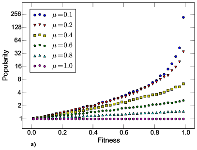
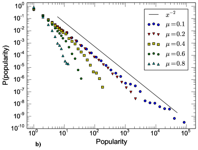
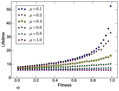
Figure 1: a) Average popularity as a function of fitness in the QBC model on an annealed random regular graph with degree distribution $P(k)=\delta_{k,1}$ for different values of $\mu$ with fixed $\alpha=10$ and $N_{u}=10^{3}$. Averages are performed over $10^{5}$ memes. b) Popularity probabilities for the same system. c) Average lifetime for the same system. d) Lifetime PDF for the same system.

The overall picture remains the same even if the contact pattern is an annealed random regular graph where each node has a single connection. This suggests that a mean-field approach, which effectively considers a regular annealed network as contact pattern, may provide an accurate description of the model dynamics.

IV A microscopic approach

We focus now on the behavior of an individual meme of fitness $f$. We define as $0\leq N_{ij}(t)\leq\alpha$ the position of meme $i$ in the memory of agent $j$ at time $t$: $N_{ij}=\alpha$ corresponds to the top position (a newly created or transmitted meme), while $N_{ij}=1$ means that the meme is about to be forgotten. If meme $i$ does not appear in the memory of agent $j$, then $N_{ij}=0$. We neglect the case in which an agent has more copies of the same meme in his feed. The quantity $N_{i}(t)=\sum_{j}N_{ij}(t)$ cumulates the positions of the meme in all users’ feeds, thus providing information about its overall diffusion. For simplicity we assume that each user is in contact with a single randomly chosen other user and that, when with probability $\mu$ a user produces a new meme, she simply puts it on top of her memory, without immediately sharing it. For the same reason we assume that, when an existing meme is selected for transmission, it is left in the original position in the transmitter feed, without putting it at the top ot the memory. We checked that both these assumption have negligible effects. The quantity $N_{i}(t)$ performs over time a one dimensional random-walk in the interval $[0,\alpha N_{u}]$. $N_{i}=0$ is an absorbing boundary condition (after extinction a meme will never reappear) and $N_{i}=\alpha N_{u}$ is a semireflecting boundary (because of our approximation, if the meme is in the first position of all feeds, $N_{i}$ cannot grow further). The initial condition is $N_{i}=\alpha$. At each time step the elementary events are:

$$N_{i}(t)=\left\{\begin{array}[]{lcl}n\rightarrow n+\alpha&&\textrm{with prob. $R_{n}$}\\ n\rightarrow n-1&&\textrm{with prob. $L_{n}$}\\ n\rightarrow n&&\textrm{with prob. $S_{n}=1-R_{n}-S_{n}$}.\end{array}\right.$$ (1)

Apart from different expressions close to the boundaries (see SM for details), the probabilities are:

$$R_{n}=(1-\mu)\frac{C_{n}}{N_{u}}\left(1-\frac{C_{n}}{N_{u}}\right)\frac{f}{\alpha},$$ (2)

and

$$L_{n}=\frac{C_{n}}{N_{u}}.$$ (3)

where $f$ is the fitness of the considered meme and $C_{n}$ is the number of individuals possessing $i$ in their memory.

Eq. (2) is derived based on the consideration that $N_{i}$ is increased by $\alpha$ if a transmission event takes place (it happens with probability $1-\mu$), if meme $i$ is present in the feed of the transmitting user (probability $C_{n}/N_{u}$) and not present in the feed of the receiver $\left(1-C_{n}/N_{u}\right)$ and if meme $i$ is selected for transmission among all memes in the feed. This last event occurs with probability $f_{i}/\sum\limits_{j\in M_{u}}f_{j}$, which we approximate with $f/\alpha$. $C_{n}$ is the number of individuals possessing $i$ in their memory, that we approximate as

$$C_{n}=\left\lfloor\frac{n+\alpha-1}{\alpha}\right\rfloor\;,$$ (4)

where $\lfloor x\rfloor$ represents the integer part (floor) of $x$.

With regard to $L_{n}$, the value of $N_{i}(t)$ decreases because the insertion of a new meme in a user feed causes the downward shift of all other memes. The insertion occurs at each time step, irrespective of whether the inserted meme is new or transmitted. Hence $L_{n}=\frac{C_{n}}{N_{u}}$, the likelihood that meme $i$ is present in the involved memory. From the expressions of the probabilities it is immediately clear that nothing depends on $f$ and $\mu$ separately, but only through the combination $\beta=(1-\mu)f$.

We simulate numerically this random walk description of meme dynamics. In the SM we show that the popularity and lifetime distributions obtained match very closely those found for the original QBC model.

In order to make the analytical treatment easier, we further simplify the random-walk description. In particular, we remove the floor function from Eq. (4), we set equal to $1$ the term $\left(1-C_{n}/N_{u}\right)$ in Eq. (2) and we introduce a numerical constant $\gamma=(\alpha+1)\frac{\alpha N_{u}+\alpha-1}{\alpha^{2}N_{u}}$ in the denominator of Eq. (4). See the SM for the justification of these modifications. Again we numerically check the distributions generated by this simplified random-walk description and find (see SM) that they are essentially equal to those of the original QBC dynamics.

At this point we can write down the master equation for the modified random walk, which reads

$$P_{n}(t+\Delta t)=S_{n}P_{n}(t)+L_{n+1}P_{n+1}(t)+R_{n-\alpha}P_{n-\alpha}(t)$$ (5a)

$$P_{\alpha N_{u}}(t+\Delta t)=(1-\mu)P_{\alpha N_{u}}(t)+\sum\limits_{j=0}^{j=\alpha}R_{\alpha N_{u}-j}P_{\alpha N_{u}-j}(t)$$ (5b)

where Equation (5a) holds for $n=0,1,...\ \alpha N_{u}-1$ provided one considers $R_{n-\alpha}=0$ for $n=0,1,...\ \alpha$ and $\Delta t=N_{u}^{-1}$.

By setting $x_{n}\equiv n/(\gamma\alpha N_{u})$ with $x_{n}$ ranging between $0$ and $1/\gamma$ and taking the thermodynamic limit $N_{u}\rightarrow\infty$, from the master equation we obtain (see SM) the Fokker-Planck (FP) equation for the probability $\rho(x,t)$ that the walker is in position $x$ at time $t$:

$$\frac{\partial}{\partial t}\rho(x,t)=\frac{1-\beta}{\gamma\alpha}\frac{\partial}{\partial x}x\rho(x,t)+\frac{1+\beta\alpha}{2\gamma^{2}\alpha^{2}N_{u}}\frac{\partial^{2}}{\partial x^{2}}x\rho(x,t)\;.$$ (6)

For large $N_{u}$ we have $\gamma=(\alpha+1)/\alpha$.

IV.1 Purely diffusive dynamics

In the limit $\beta\rightarrow 1$ the drift term in Eq. (6) vanishes. We are left with the FP equation of a purely diffusive stochastic process:

$$\frac{\partial}{\partial t}\rho(x,t)=D_{0}\frac{\partial^{2}}{\partial x^{2}}x\rho(x,t)\;,$$ (7)

where

$$D_{0}=\frac{1+\alpha}{2\gamma^{2}\alpha^{2}N_{u}}=\frac{1}{2(1+\alpha)N_{u}},$$ (8)

which differs from standard diffusion because of the space-dependent diffusion coefficient. The limit $\mu\rightarrow 0$ changes also the boundary conditions: the boundary in $x=1/\gamma$ is semireflecting because $N_{i}(t)=N_{u}\alpha$ can decrease with probability $\mu$ or remain unchanged, with probability $1-\mu$. Thus in the case $\mu=0$ both the boundary condition in $x=0$ and in $x=\gamma^{-1}$ are absorbing: $\rho(0,t)=\rho(\gamma^{-1},t)=0$. The initial condition is $\rho(x,t=0)=\delta(x-x_{\alpha})$ with $x_{\alpha}=1/(\gamma N_{u})$.

It is possible to find the solution of this equation as an eigenfunction expansion of the operator $\mathcal{L}_{FP}=D_{0}\frac{\partial^{2}}{\partial x^{2}}x$ (see SM for details), obtaining:

$$\rho(x,t)=\frac{\pi^{2}\gamma}{2}\sqrt{\frac{x_{\alpha}}{x}}\sum_{n=1}^{\infty}nJ_{1}(\pi n\sqrt{\gamma x_{\alpha}})J_{1}(\pi n\sqrt{\gamma x})e^{-t/\tau_{n}}\;,$$ (9)

where $J_{1}(z)$ is a Bessel function of the first kind. The characteristic time scale of each eigenfunction is

$$\tau_{n}=\frac{8\gamma\alpha^{2}N_{u}}{(1+\alpha)j_{1,n}^{2}}\simeq\frac{8\alpha N_{u}}{\pi^{2}n^{2}}.$$ (10)

where the $j_{1,n}$, the zeros of $J_{1}(z)$, are approximated as $j_{1,n}=\pi n$. Using this expression, it is possible to compute (see SM for details) the survival probability in the limit $\mu\rightarrow 0$, which turns out to be

$$S(t)\simeq\left\{\begin{array}[]{lcl}1&&t\ll\alpha\\ \alpha t^{-1}e^{-t/\tau}&&t\gg\alpha\end{array}\right.$$ (11)

where $\tau=8\alpha N_{u}/\pi^{2}$ is $\tau_{1}$ after the approximation $j_{1,n}\rightarrow\pi n$ is made. Based on this result the lifetime distribution can be computerd (see SM). In the limit of large $N_{u}$, i.e., diverging $\tau$, it reads

$$F(l)\!=\!-\left.\frac{dS}{dt}\right|_{t=l}\!\simeq\!\left\{\!\begin{array}[]{lr}\!0&l\ll\alpha\\ \alpha l^{-2}&l\gg\alpha\end{array}\right.$$ (12)

This expression of $F(l)$ accounts for the most important feature observed in simulations: for $l\ll\tau$ (notice that $\tau$ diverges with $N_{u}$) the distribution decays as a power-law with exponent $\eta_{l}=2$. Simulations of the QBC model with all memes having fitness $f=1$ agree with this analytical prediction (see Fig. 2).

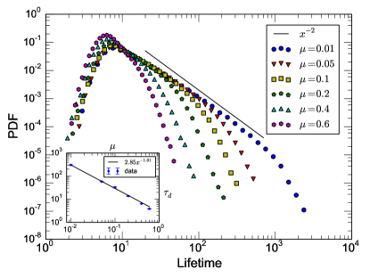
Figure 2: Main: Lifetime PDF for fixed $\alpha=10$ and $N_{u}=10^{3}$ obtained by simulating the QBC model on an annealed regular network with degree 1 and fixed fitness $f=1$. The solid straight line is a power-law with exponent $-2$. Inset: Symbols are the temporal scale $\tau_{d}$ over which the PDF decays, estimated numerically by fitting the exponential tails in the main. The straight line is a power-law fit to the numerical values of $\tau_{d}$, confirming that $\tau_{d}$ is inversely proportional to $\mu$ for $f=1$ [see Eq. (14)].

By means of the standard argument connecting the exponents of power-law tails for scaling variables (see SM) it is possible to relate $\eta_{l}$ with the analogous exponent $\eta_{p}$ for the popularity distribution: $\eta_{l}=s(\eta_{p}-1)+1$, where $p\sim l^{s}$. Simulations yield a value close to $s=2$, from which $\eta_{p}=3/2$, in good agreement with simulations (see SM).

IV.2 Pure drift

The opposite limit for the FP equation (6) is the pure drift case, which always holds in the large $N_{u}$ limit, as $D_{0}\propto N_{u}^{-1}$, unless $\mu=0$ and $f=1$:

$$\frac{\partial}{\partial t}\rho(x,t)=\frac{1}{\tau_{d}}\frac{\partial}{\partial x}x\rho(x,t)$$ (13)

where

$$\frac{1}{\tau_{d}}=\frac{1-\beta}{\gamma\alpha}=[1-(1-\mu)f](\alpha+1).$$ (14)

This equation describes a deterministic motion

$$x(t)=x_{\alpha}e^{-t/\tau_{d}}\;,$$ (15)

i.e., the meme position drifts exponentially toward $x=0$; in other words the systematic drift attracts walkers toward the absorbing boundary. This introduces an additional exponential cutoff in the lifetime distribution, which can be globally written as

$$F(l)\propto\alpha l^{-2}e^{-l/\tau_{d}}$$ (16)

in agreement with simulations (see Fig. 2, inset).

IV.3 Average over the fitness

In the original definition of the QBC model the fitness is a random variable uniformly distributed between $0$ and $1$. Using Eq. (16) it is possible to compute the lifetime distribution also in this case, by averaging over $f$ (see SM) and obtaining, in the limit $\mu\rightarrow 0$:

$$F_{\langle f\rangle}(l)\approx\alpha(\alpha+1)l^{-3}\left[1-e^{-(\alpha+1)l}\right]\;.$$ (17)

The exponent of the lifetime distribution is then $\eta_{l}=3$, in reasonable agreement with Fig. 1. A similar conclusion can be drawn for the popularity distribution, predicted to decay as $p^{-2}$.

In summary, by means of a mapping of QBC dynamics onto a random-walk description, we have derived expressions for for the lifetime and popularity distributions, which account for the phenomenology observed in numerical simulations.

V A macroscopic approach

The microscopic approach allows to determine the dependence of the average lifetime on the fitness and hence estimate the average number $N_{f}$ of memes with given $f$ in the steady state. However, the same quantities can be derived much more easily by a simple approach of mean-field type, focused directly on the temporal evolution of the $N_{f}$. For simplicity we assume that fitness values are discretized in $F$ classes and, again, that the degree of each agent is 1. We define $N_{f}(t)$ as the average number of memes with fitness $f$ present in the system at time $t$. This quantity changes over time because of two possible gain and two possible loss processes. The creation of a new meme, occurring at rate $\mu$, increases $N_{f}$ by 1 with a probability $1/F$ (if the created meme has exactly fitness $f$), but it may also reduce $N_{f}$ by 1 if the agent creating the new meme forgets a meme of fitness $f$. This last event occurs with probability $N_{f}/(N_{u}\alpha)$. The transmission of an existing meme, occurring at rate $1-\mu$, increases $N_{f}$ if the transmitting agent has a meme with fitness $f$ in her feed (probability proportional to $N_{f}$) and the meme is selected (probability proportional to $f$). Overall the normalized probability of the event is $fN_{f}/[\sum_{f^{\prime}}f^{\prime}N_{f^{\prime}}]$. Finally also the transmission event may lead to an agent forgetting a meme with fitness $f$ with probability $N_{f}/(N_{u}\alpha)$. The temporal evolution of the $N_{f}$ is then given by the set of coupled equations

$$\!\dot{N}_{f}(t)\!=\!\!\mu\!\left[\frac{1}{F}-\frac{N_{f}(t)}{N}\right]+(1-\mu)\!\left[\frac{fN_{f}(t)}{\sum_{f^{\prime}}f^{\prime}N_{f^{\prime}}(t)}-\frac{N_{f}(t)}{N}\!\right]\!.$$ (18)

which conserves the total number $\sum_{f^{\prime}}N_{f^{\prime}}$. Straightforward numerical integration of Eq. (18) allows to determine the stationary values of the $N_{f}$ and hence of the densities $n_{f}=N_{f}/(N_{u}\alpha/F)$, where $N_{u}\alpha/F$ is the average number of memes with fitness $f$ if all $F$ classes were populated uniformly. The comparison with the outcome of numerical simulations (see Fig. 3)

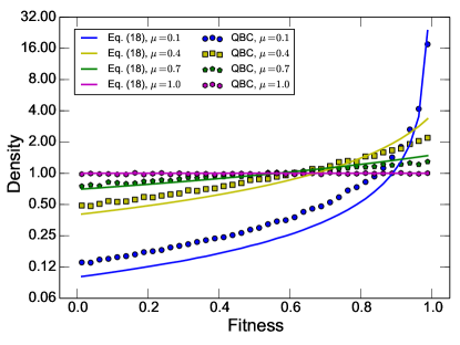
Figure 3: Comparison between the average density of memes in the QBC model (symbols) and the stationary solutions of Eq. (18) (lines) for different values of $\mu$. $N_{u}=10^{3}$, $\alpha=10$, $F=40$. Averages are computed over $10^{5}$ memes.

confirms a satisfactory agreement.

VI Conclusions

In this paper we have studied the model for information diffusion recently introduced in Ref. Qiu et al. (2017). We have been able to derive analytically the lifetime distribution and other properties for a simplified version of the dynamics, which reproduces the phenomenology of the original model.

Our treatment of the QBC model allows to understand how broad tails in the lifetime and popularity distributions, observed empirically, arise. A power-law distribution with an exponent $\eta_{p}\approx 2$ is in agreement with the observations of Ref. Qiu et al. (2017), where hashtags are used to identify Twitter memes. On the other hand, other studies using hashtags give quite different results from the QBC model predictions. In Ref. Weng et al. (2012) a power-law decay for meme lifetime has been observed, with an exponent $\eta_{l}\approx 2.5$. This value is not far but distinct from the value $\eta_{l}$ predicted by the QBC model in the case of uniformly distributed fitness. Moreover, the strong correlation between meme lifetime and popularity (see SM) is not observed in Twitter data Baños et al. (2013); Gleeson et al. (2016), even if proxies different from hashtags are used to identify memes González-Bailón et al. (2011). A stringent empirical validation of models of online information spreading is itself a difficult task because of the apparent lack of universality. Referring to Twitter data, the identification of memes as URLs leads to a lognormal distribution of popularity Lerman and Ghosh (2010), the analysis of retweet cascades leads to a size distribution with exponent $\eta_{s}\approx 2.3$ Wegrzycki et al. (2017) with possibly an exponential cutoff Vosoughi et al. (2018) and reply trees give $\eta_{s}\approx 4$ Nishi et al. (2016). Looking at other data sources, the landscape is even more varied: the popularity distribution, estimated from Facebook data, exhibits a power-law deacy with exponent $\eta_{p}\approx 2.1$ Cheng et al. (2014), while popularity-lifetime correlations are shown to be different between Digg and Youtube data Szabo and Huberman (2010). One could easily change, within the QBC model, the fitness distribution to achieve a better agreement with these observations. In any case it is clear that the QBC model is a gross oversimplification of the real meme diffusion process in online social media. To make the QBC dynamics less unrealistic several hypotheses underlying the present version of model could be lifted. Some of them, such as a nonuniform fitness distribution or a nonlinear dependence on $f$ of the probability of selecting a meme, can be easily treated within the present analytical approach. Other fundamental generalizations, such as agent-dependent values of $\alpha$ and $\mu$ or heterogeneous rates of individual activation, can be investigated by means of straightforward numerical simulations. One of the ingredients adding realism to the QBC dynamics is the consideration of agents that do not accept in their feeds (and thus do not spread further) memes they have already seen in the past. The effect of this long-term memory is briefly discussed in the SM, but the main result is the change of the popularity and lifetime distributions, that lose their power-law tail. At a more general level, one of the weak points of the QBC model is its insensitivity with respect to changes of the contact pattern topology. While this feature allows our mean-field approach to be successful, empirical data contradict this result: one of the main pieces of evidence is the existence of influential spreaders, i.e. users which, because of their position in the social network have a disproportionate effect on meme dynamics Bakshy et al. (2011); Baños et al. (2013); Borge-Holthoefer et al. (2012). The investigation of increasingly sophisticated models for information spreading and the comparison with the ever larger body of empirical data available remains a challenging avenue for future research.

References

- Howell et al. (2013) L. Howell et al., WEF Report 3, 15 (2013).
- Del Vicario et al. (2016) M. Del Vicario, A. Bessi, F. Zollo, F. Petroni, A. Scala, G. Caldarelli, H. E. Stanley, and W. Quattrociocchi, Proceedings of the National Academy of Sciences 113, 554 (2016).
- Vosoughi et al. (2018) S. Vosoughi, D. Roy, and S. Aral, Science 359, 1146 (2018).
- Kwak et al. (2010) H. Kwak, C. Lee, H. Park, and S. Moon, in Proceedings of the 19th International Conference on World Wide Web (ACM, New York, NY, USA, 2010), WWW ’10, pp. 591–600.
- Lerman and Ghosh (2010) K. Lerman and R. Ghosh, in in Proc. 4th Int. Conf. on Weblogs and Social Media (ICWSM) (2010), pp. 90–97.
- González-Bailón et al. (2011) S. González-Bailón, J. Borge-Holthoefer, A. Rivero, and Y. Moreno, Scientific Reports 1, 197 (2011), article.
- Bakshy et al. (2011) E. Bakshy, J. M. Hofman, W. A. Mason, and D. J. Watts, in Proceedings of the Fourth ACM International Conference on Web Search and Data Mining (ACM, New York, NY, USA, 2011), WSDM ’11, pp. 65–74.
- Baños et al. (2013) R. A. Baños, J. Borge-Holthoefer, and Y. Moreno, EPJ Data Science 2, 6 (2013).
- Cheng et al. (2014) J. Cheng, L. Adamic, P. A. Dow, J. M. Kleinberg, and J. Leskovec, in Proceedings of the 23rd International Conference on World Wide Web (ACM, New York, NY, USA, 2014), WWW ’14, pp. 925–936.
- Nishi et al. (2016) R. Nishi, T. Takaguchi, K. Oka, T. Maehara, M. Toyoda, K.-i. Kawarabayashi, and N. Masuda, Social Network Analysis and Mining 6, 26 (2016).
- Pramanik et al. (2017) S. Pramanik, Q. Wang, M. Danisch, J.-L. Guillaume, and B. Mitra, Social Network Analysis and Mining 7, 41 (2017).
- Wegrzycki et al. (2017) K. Wegrzycki, P. Sankowski, A. Pacuk, and P. Wygocki, in Proceedings of the 26th International Conference on World Wide Web (International World Wide Web Conferences Steering Committee, Republic and Canton of Geneva, Switzerland, 2017), WWW ’17, pp. 569–576.
- Castellano et al. (2009) C. Castellano, S. Fortunato, and V. Loreto, Rev. Mod. Phys. 81, 591 (2009).
- Buchanan (2007) M. Buchanan, The social atom (Bloomsbury, New York, NY, USA, 2007).
- Wu and Huberman (2007) F. Wu and B. A. Huberman, Proceedings of the National Academy of Sciences 104, 17599 (2007).
- Weng et al. (2012) L. Weng, A. Flammini, A. Vespignani, and F. Menczer, Scientific Reports 2, 335 (2012).
- Gleeson et al. (2014) J. P. Gleeson, J. A. Ward, K. P. O’Sullivan, and W. T. Lee, Phys. Rev. Lett. 112, 048701 (2014).
- Gleeson et al. (2016) J. P. Gleeson, K. P. O’Sullivan, R. A. Baños, and Y. Moreno, Phys. Rev. X 6, 021019 (2016).
- Qiu et al. (2017) X. Qiu, D. F. M. Oliveira, A. Sahami Shirazi, A. Flammini, and F. Menczer, Nature Human Behaviour 1, 0132 (2017).
- Pastor-Satorras et al. (2015) R. Pastor-Satorras, C. Castellano, P. Van Mieghem, and A. Vespignani, Rev. Mod. Phys. 87, 925 (2015).
- Szabo and Huberman (2010) G. Szabo and B. A. Huberman, Communications of the ACM 53, 80 (2010).
- Borge-Holthoefer et al. (2012) J. Borge-Holthoefer, A. Rivero, and Y. Moreno, Physical review E 85, 066123 (2012).