Group Sparsity Residual with Non-Local Samples for Image Denoising

Abstract

Inspired by group-based sparse coding, recently proposed group sparsity residual (GSR) scheme has demonstrated superior performance in image processing. However, one challenge in GSR is to estimate the residual by using a proper reference of the group-based sparse coding (GSC), which is desired to be as close to the truth as possible. Previous researches utilized the estimations from other algorithms (i.e., GMM or BM3D), which are either not accurate or too slow. In this paper, we propose to use the Non-Local Samples (NLS) as reference in the GSR regime for image denoising, thus termed GSR-NLS. More specifically, we first obtain a good estimation of the group sparse coefficients by the image nonlocal self-similarity, and then solve the GSR model by an effective iterative shrinkage algorithm. Experimental results demonstrate that the proposed GSR-NLS not only outperforms many state-of-the-art methods, but also delivers the competitive advantage of speed.

Index Terms—  Image denoising, group-based sparse coding, group sparsity residual, nonlocal self-similarity, iterative shrinkage algorithm.

1 Introduction

Image denoising plays an important role in various image processing tasks. In general, image denoising aims to restore the clean image y from its corrupted observation $\textbf{\emph{z}}=\textbf{\emph{y}}+\textbf{\emph{v}}$, where v is usually considered to be an additive white Gaussian noise. Image denoising problem is mathematically ill-posed and priors are thus usually employed to achieve good results. Over the past few years, numerous image prior models have been developed, including total variation based [1, 2], wavelet/curvelet based [3, 4, 40, 5], sparse coding based [6, 7], nonlocal self-similarity based [8, 9, 12], and deep learning based [10, 11] ones.

One significant advance in image processing is to model the prior on patches, and a representative research is sparse coding [6, 7], which assumes that each patch of an image can be precisely modeled by a sparse linear combination of some fixed and trainable basis elements, which are therefore called atoms and these atoms compose a dictionary. The seminal work of K-SVD dictionary learning method [7] has not only shown promising denoising performance, but also been extended to other image processing and computer vision tasks [13, 14]. Meanwhile, since image patches with similar structures can be spatially far from each other and thus can be collected across the whole image, the so-called nonlocal self-similarity (NSS) prior is among the most remarkable priors for image restoration [9, 15, 16, 17, 18, 19, 20, 21, 22, 23, 24]. The seminal work of nonlocal means (NLM) [8] exploited the NSS prior to carry out a form of the weighted filtering for image denoising. Compared with the local regularization methods (e.g, total variation based method [1]), the nonlocal regularization based methods can retain the image edges and the sharpness effectively. Inspired by the success of the NSS prior, group-based sparse coding (GSC) has attracted considerable interests in image denoising [17, 18, 21, 22, 23, 24]. However, due to the influence of noise, the conventional GSC model is accurate enough to restore the original image.

Most recently, the group sparsity residual [31, 32] has been proposed for image denoising, which adopts a reference in each iteration to approximate the true sparse coefficients of each group. The reference was estimated by Gaussian mixture model (GMM) [34, 22] or other algorithms, which is either not accurate or too slow. In this paper, we propose a new method for image denoising via group sparsity residual scheme with non-local samples (GSR-NLS). We first obtain a good estimation of the group sparse coefficients of the original image by the image nonlocal self-similarity, and then the group sparse coefficients of the noisy image are inferred to approximate this estimation. Moreover, we develop an effective iterative shrinkage algorithm to solve the proposed GSR-NLS model. Experimental results show that the proposed GSR-NLS not only outperforms many state-of-the-art methods in terms of the objective and the perceptual metrics, but also deliveries a competitive speed.

2 Group-based Sparse Coding for Image Denoising

In this section, we will briefly introduce the conventional group-based sparse coding (GSC) model for image denoising. Specifically, taking a clean image $\textbf{\emph{y}}\in{\mathbb{R}}^{\sqrt{N}\times\sqrt{N}}$ as an example, it is divided into $n$ overlapped patches of size $\sqrt{b}\times\sqrt{b}$, and each patch is denoted by a vector $\textbf{\emph{y}}_{i}\in{\mathbb{R}}^{b}$, $i=1,2,...n$. Then for each patch $\textbf{\emph{y}}_{i}$, its $m$ similar patches are selected from a searching window with $W\times W$ pixels to form a set ${\cal S}_{i}$. Following this, all patches in ${\cal S}_{i}$ are stacked into a matrix $\textbf{\emph{Y}}_{i}\in{\mathbb{R}}^{b\times m}$, i.e., $\textbf{\emph{Y}}_{i}=\{\textbf{\emph{y}}_{i,1},\textbf{\emph{y}}_{i,2},...,\textbf{\emph{y}}_{i,m}\}$. The matrix $\textbf{\emph{Y}}_{i}$ consisting of patches with similar structures is thereby called a group, where $\{\textbf{\emph{y}}_{i,j}\}_{j=1}^{m}$ denotes the $j$-th patch in the $i$-th group. Following this, similar to patch-based sparse coding [6, 7], given a dictionary $\textbf{\emph{D}}_{i}$, each group $\textbf{\emph{Y}}_{i}$ can be sparsely represented and solved by the following minimization problem,

$$\textstyle{{{\textbf{\emph{B}}}_{i}}=\arg\min_{{\textbf{\emph{B}}}_{i}}\left(||{\textbf{\emph{Y}}}_{i}-{\textbf{\emph{D}}}_{i}{{\textbf{\emph{B}}}_{i}}||_{F}^{2}+\lambda||{{\textbf{\emph{B}}}_{i}}||_{1}\right)},$$ (1)

where $\lambda$ is the regularization parameter; $||~{}||_{F}^{2}$ denotes the Frobenious norm. Here, $\ell_{1}$-norm is imposed on each column of ${{\textbf{\emph{B}}}_{i}}$, which also holds true for the following derivation with $\ell_{1}$-norm on matrix.

In image denoising, each patch $\textbf{\emph{z}}_{i}$ is extracted from the noisy image z, and we search for its $m$ similar patches to generate a noisy image patch group $\textbf{\emph{Z}}_{i}\in{\mathbb{R}}^{b\times m}$, i.e., $\textbf{\emph{Z}}_{i}=\{\textbf{\emph{z}}_{i,1},\textbf{\emph{z}}_{i,2},...,\textbf{\emph{z}}_{i,m}\}$. Then, image denoising is translated into how to restore the $\textbf{\emph{Y}}_{i}$ from $\textbf{\emph{Z}}_{i}$ using the GSC model,

$$\textstyle{{{\textbf{\emph{A}}}_{i}}=\arg\min_{{\textbf{\emph{A}}}_{i}}\left(||{\textbf{\emph{Z}}}_{i}-{\textbf{\emph{D}}}_{i}{{\textbf{\emph{A}}}_{i}}||_{F}^{2}+\lambda||{{\textbf{\emph{A}}}_{i}}||_{1}\right)}.$$ (2)

Once all group sparse codes $\{\textbf{\emph{A}}_{i}\}_{i=1}^{n}$ are obtained, the underlying clean image $\hat{\textbf{\emph{y}}}$ can be reconstructed as $\hat{\textbf{\emph{y}}}=\textbf{\emph{D}}\textbf{\emph{A}}$, where A denotes the set of $\{\textbf{\emph{A}}_{i}\}_{i=1}^{n}$. However, due to the noise, the conventional GSC mode of Eq. (2) cannot recover the underlying image y accurately.

3 Denoising via Group Sparsity Residual with Non-Local Samples

Recalling Eq. (1) and Eq. (2), the noisy group sparse coefficient $\textbf{\emph{A}}_{i}$ obtained by solving Eq. (2) is excepted to be as close to the true group sparse coefficient $\textbf{\emph{B}}_{i}$ of the original image y in Eq. (1) as possible. Accordingly, the quality of image denoising largely depends on the group sparsity residual, which is defined as the difference between the noisy group sparse coefficient $\textbf{\emph{A}}_{i}$ and the true group sparse coefficient $\textbf{\emph{B}}_{i}$,

$$\textstyle{{{\textbf{\emph{R}}}_{i}}={{\textbf{\emph{A}}}_{i}}-{{\textbf{\emph{B}}}_{i}}}.$$ (3)

In order to obtain a good performance in image denoising, we hope that the group sparsity residual ${{\textbf{\emph{R}}}_{i}}$ of each group is as small as possible. To this end, to reduce the group sparsity residual ${{\textbf{\emph{R}}}}=\{{{\textbf{\emph{R}}}_{i}}\}_{i=1}^{n}$ and boost the accuracy of A, we propose the group sparsity residual (GSR) based model for image denoising. This is

$$\textstyle{{{\textbf{\emph{A}}}_{i}}=\arg\min_{{\textbf{\emph{A}}}_{i}}\left(||{\textbf{\emph{Z}}}_{i}-{\textbf{\emph{D}}}_{i}{{\textbf{\emph{A}}}_{i}}||_{F}^{2}+\lambda||{{\textbf{\emph{A}}}_{i}}-{{\textbf{\emph{B}}}_{i}}||_{p}\right)},$$ (4)

Similarly, $\ell_{p}$-norm is imposed on each column of ${{\textbf{\emph{R}}}_{i}}$, which also holds true for the following derivation with $\ell_{p}$-norm on matrix. Since the original image y is not available, it is impossible to get the true sparse coefficient ${{\textbf{\emph{B}}}_{i}}$. We will describe how to estimate ${{\textbf{\emph{B}}}_{i}}$ and $p$ below.

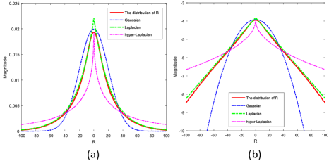
Fig. 1: The distribution of the group sparsity residual R for image House with $\sigma$=30 and fitting Gaussian, Laplacian and hyper-Laplacian distribution in (a) linear and (b) log domain, respectively.

3.1 Determine $p$

Let us come back to Eq. (4), it is clear that one important problem of the proposed GSR based image denoising is the determination of $p$. Here, we conduct some experiments to investigate the statistical property of ${{\textbf{\emph{R}}}}=\{\textbf{\emph{R}}_{i}\}_{i=1}^{n}$. We compute ${{\textbf{\emph{A}}}}=\{\textbf{\emph{A}}_{i}\}_{i=1}^{n}$ and ${{\textbf{\emph{B}}}}=\{\textbf{\emph{B}}_{i}\}_{i=1}^{n}$ by solving Eq. (2) and Eq. (1), respectively. The principe component analysis (PCA) based dictionary [15] is used in these experiments. One typical image House is used as example, where Gaussian white noise is added with standard deviation $\sigma_{n}=30$. We plot the empirical distribution of R as well as the fitting Gaussian, Laplacian and hyper-Laplacian distributions in Fig. 1 (a). To better observe the fitting of the tails, we also plot these distributions in the log domain in Fig. 1 (b). It can be seen that the empirical distribution of R can be well characterized by the Laplacian distribution. Therefore, we set $p=1$ and thus the $\ell_{1}$-norm is adopted to regularize the proposed GSR model,

$$\textstyle{{{\textbf{\emph{A}}}_{i}}=\arg\min_{{\textbf{\emph{A}}}_{i}}\left(||{\textbf{\emph{Z}}}_{i}-{\textbf{\emph{D}}}_{i}{{\textbf{\emph{A}}}_{i}}||_{F}^{2}+\lambda||{{\textbf{\emph{A}}}_{i}}-{{\textbf{\emph{B}}}_{i}}||_{1}\right)}.$$ (5)

3.2 Estimate of the Unknown Group Sparse Coefficient B

Since the original image y is not available in real applications, the true group sparse coefficient $\textbf{\emph{B}}_{i}$ is unknown. Thus, we need to estimate $\textbf{\emph{B}}_{i}$ in Eq. (5). In general, there are a variety of methods to estimate $\textbf{\emph{B}}_{i}$, which depends on the prior knowledge of the original image y. Different from [31, 32], in this paper, based on the fact that natural images often contain repetitive structures [28], we search nonlocal similar patches (i.e., non-local samples) to the given patch and use the method similar to nonlocal means [8] to estimate $\textbf{\emph{B}}_{i}$. Specifically, a good estimation of $\textbf{\emph{b}}_{i,1}$ can be computed by the weighted average of each element $\textbf{\emph{a}}_{i,j}$ in $\textbf{\emph{A}}_{i}$ associated with each group including $m$ nonlocal similar patches, where $\textbf{\emph{b}}_{i,1}$ and $\textbf{\emph{a}}_{i,j}$ represent the first and the $j$-th element of $\textbf{\emph{B}}_{i}$ and $\textbf{\emph{A}}_{i}$, respectively. Then we have,

$$\textstyle{\textbf{\emph{b}}_{i,1}=\sum\nolimits_{j=1}^{m}w_{i,j}\textbf{\emph{a}}_{i,j}},$$ (6)

where $w_{i,j}$ is the weight, which is inversely proportional to the distance between patches $\textbf{\emph{z}}_{i}$ and $\textbf{\emph{z}}_{i,j}$: $w_{i,j}={\rm exp}(-||\textbf{\emph{z}}_{i}-\textbf{\emph{z}}_{i,j}||_{2}^{2}/h/L)$, where $h$ is a predefined constant and $L$ is a normalization factor [8]. After this, we simply copy $\textbf{\emph{b}}_{i,1}$ by $m$ times to estimate $\textbf{\emph{B}}_{i}$, i.e.,

$$\textstyle{\textbf{\emph{B}}_{i}=\{\textbf{\emph{b}}_{i,1},\textbf{\emph{b}}_{i,2},...,\textbf{\emph{b}}_{i,m}\}},$$ (7)

where $\{\textbf{\emph{b}}_{i,j}\}_{j=1}^{m}$ denotes the $j$-th element in the $i$-th group sparse coefficient $\textbf{\emph{B}}_{i}$ and they are the same. The flowchart of the proposed GSR-NLS model for image denoising is illustrated in Fig. 2. Another important issue of the proposed GSR-NLS based image denoising is the selection of the dictionary. To adapt to the local image structures, instead of learning an over-complete dictionary for each group $\textbf{\emph{Z}}_{i}$ as in [23], we utilized the PCA based dictionary [15].

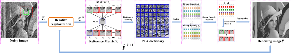
Fig. 2: The flowchart of the proposed GSR-NLS model for image denoising.

3.3 Iterative Shrinkage Algorithm to Solve the Proposed GSR-NLS Model

Due to orthogonality (obtained by PCA) of each dictionary $\textbf{\emph{D}}_{i}$, Eq. (5) can be rewritten as

$${{\textbf{\emph{A}}}_{i}} =\textstyle{\arg\min_{{\textbf{\emph{A}}}_{i}}\{||{\textbf{\emph{G}}}_{i}-{{\textbf{\emph{A}}}_{i}}||_{F}^{2}+\lambda||{{\textbf{\emph{A}}}_{i}}-{{\textbf{\emph{B}}}_{i}}||_{1}\}}$$ (8)

$$=\textstyle{\arg\min_{{\boldsymbol{\alpha}}_{i}}\{||{{\textbf{\emph{g}}}}_{i}-{{\boldsymbol{\alpha}}_{i}}||_{2}^{2}+\lambda||{{\boldsymbol{\alpha}}_{i}}-{{\boldsymbol{\beta}}_{i}}||_{1}\}},$$

where $\textbf{\emph{Z}}_{i}=\textbf{\emph{D}}_{i}\textbf{\emph{G}}_{i}$; ${{\boldsymbol{\alpha}}_{i}}$, ${{\boldsymbol{\beta}}_{i}}$ and ${{\textbf{\emph{g}}}}_{i}$ denote the vectorization of the matrix ${{\textbf{\emph{A}}}_{i}}$, ${{\textbf{\emph{B}}}_{i}}$ and ${{\textbf{\emph{G}}}_{i}}$, respectively.

To solve Eq. (8) effectively, an iterative shrinkage algorithm [29] is adopted. To be concrete, for fixed ${{\textbf{\emph{g}}}}_{i}$, ${{\boldsymbol{\beta}}_{i}}$ and $\lambda$, we have

$$\textstyle{\hat{{\boldsymbol{\alpha}}}_{i}={\rm soft}({{\textbf{\emph{g}}}}_{i}-{{\boldsymbol{\beta}}_{i}},\lambda)+{{\boldsymbol{\beta}}_{i}}},$$ (9)

where soft ($\cdot$) is the soft-thresholding operator [29].

Following this, the latent clean patch group $\textbf{\emph{Y}}_{i}$ can be calculated by $\hat{\textbf{\emph{Y}}}_{i}=\textbf{\emph{D}}_{i}\hat{\textbf{\emph{A}}}_{i}$. After obtaining the estimate of all groups $\{\hat{\textbf{\emph{Y}}}_{i}\}$, we get the full image $\hat{\textbf{\emph{y}}}$ by putting the groups back to their original locations and averaging the overlapped pixels. Moreover, we could execute the above denoising procedures several iterations for better results. In the $k$-th iteration, the iterative regularization strategy [2] is utilized to update the estimation of the noise variance, and thus updating $\textbf{\emph{z}}^{k}$. The standard deviation of noise in $k$-th iteration is adjusted as ${\sigma_{n}}^{k}=\eta\sqrt{{\sigma_{n}}^{2}-||\textbf{\emph{z}}-\textbf{\emph{y}}^{k-1}||_{2}^{2}}$, where $\eta$ is a constant.

The parameter $\lambda$ that balances the fidelity term and the regularization term should be adaptively determined in each iteration. Inspired by [3], the regularization parameter $\lambda$ of each noisy group $\textbf{\emph{Z}}_{i}$ is set to $\lambda=c*2\sqrt{2}{\sigma_{n}}^{2}/(\delta_{i}+\varepsilon)$, where $\delta_{i}$ denotes the estimated variance of $\textbf{\emph{R}}_{i}$ and $c,\varepsilon$ are small constants.

Throughout the numerical experiments, we choose the following stoping iteration for the proposed denoising algorithm, i.e, $||\hat{\textbf{\emph{y}}}^{k}-\hat{\textbf{\emph{y}}}^{k-1}||_{2}^{2}/||\hat{\textbf{\emph{y}}}^{k-1}||_{2}^{2}<\tau$, where $\tau$ is a small constant. The complete description of the proposed GSR-NLS for image denoising is exhibited in Algorithm 1.

Algorithm 1 The Proposed GSR-NLS for Image Denoising.

0:  Noisy image z.

1:  Initialize $\hat{\textbf{\emph{y}}}^{0}=\textbf{\emph{z}}$, $\textbf{\emph{z}}^{0}=\textbf{\emph{z}}$, $\boldsymbol{\sigma}_{n}$, $b$, $c$, $m$, $h$, $W$, $\gamma$, $\eta$, $\tau$ and $\varepsilon$.

2:  for $k=1$ to Max-Iter  do

3:     Iterative Regularization $\textbf{\emph{z}}^{k}=\hat{\textbf{\emph{y}}}^{k-1}+\gamma(\textbf{\emph{z}}-\textbf{\emph{z}}^{k-1})$.

4:     for Each patch $\textbf{\emph{z}}_{i}$ in $\textbf{\emph{z}}^{k}$ do

5:        Find nonlocal similar patches to form a group ${\textbf{\emph{Z}}}_{i}$.

6:        Constructing dictionary ${\textbf{\emph{D}}}_{i}$ by ${\textbf{\emph{Z}}}_{i}$ using PCA.

7:        Update ${\textbf{\emph{A}}}_{i}$ computing by ${\textbf{\emph{A}}}_{i}={\textbf{\emph{D}}}_{i}^{-1}{\textbf{\emph{Z}}}_{i}$.

8:        Estimate ${\textbf{\emph{B}}}_{i}$ by Eq. (6) and Eq. (7).

9:        Update $\lambda$ computing by $\lambda=c*2\sqrt{2}{\sigma_{n}}^{2}/(\delta_{i}+\varepsilon)$.

10:        Estimate $\hat{{\textbf{\emph{A}}}}_{i}$ by Eq. (9).

11:        Get the estimation: $\hat{\textbf{\emph{Y}}}_{i}=\textbf{\emph{D}}_{i}\hat{{\textbf{\emph{A}}}}_{i}$.

12:     end for

13:     Aggregate ${\textbf{\emph{Y}}}_{i}$ to form the denoised image $\hat{\textbf{\emph{y}}}^{k}$.

14:  end for

15:  Output: The final denoised image $\hat{\textbf{\emph{y}}}$.

3.4 Different from Existing Methods

Now we discuss the difference between the proposed GSR-NLS method, and NCSR [30] and our previous approaches [31, 32].

The main difference between NCSR [30] and the proposed GSR-NLS is that NCSR is essentially a patch-based sparse coding method, which usually ignored the relationship among similar patches [17, 21, 23, 33]. In addition, NCSR extracted image patches from noisy image $\textbf{\emph{z}}^{k}$ and used $K$-means algorithm to generate $K$ clusters. Following this, it learned $K$ PCA sub-dictionaries from each cluster. However, since each cluster includes thousands of patches, the dictionary learned by PCA from each cluster may not accurately centralize the image features. The proposed GSR-NLS learned the PCA dictionary from each group and the patches in each group are similar, and therefore, our PCA dictionary is more appropriate. An additional advantage of GSR-NLS is that it only requires 1/3 computational time of NCSR but achieves $\sim$0.5dB improvement on average over NCSR (see Section 4 for details).

Our previous work in [31] utilized the pre-filtering BM3D [9] to estimate B, and thus the denoising performance largely depends on the pre-filtering. In other words, if the pre-filtering cannot be used, the denoising method will fail. Our another work [32] estimated B from example image set based on GMM [34]. However, under many practical situations, the example image set is simply unavailable. Moreover, the computation speed of this method is very slow. Therefore, the proposed GSR-NLS is more reasonable and generic while providing very similar results as in [31, 32].

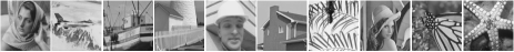
Fig. 3: The test images for denoising experiments.

Table 1: PSNR (dB) results of different denoising methods.

	$\sigma_{n}=20$										$\sigma_{n}=40$
Images	BM3D	EPLL	Plow	NCSR	PID	PGPD	aGMM	LINC	AST-	GSR-	BM3D	EPLL	NCSR	PID	PGPD	PGPD	aGMM	LINC	AST-	GSR-
									NLS	NLS									NLS	NLS
Airplane	30.59	30.60	29.98	30.50	30.71	30.80	30.54	30.57	30.70	30.87	26.88	27.08	26.70	26.78	27.25	27.12	26.95	27.08	27.10	27.21
Barbara	31.24	29.85	30.75	31.10	30.98	31.12	30.51	31.70	31.43	31.47	27.26	25.99	27.59	27.25	27.68	27.43	26.34	27.77	27.41	27.85
boats	31.42	30.87	30.90	31.26	31.27	31.38	31.20	31.52	31.50	31.55	27.76	27.42	27.55	27.52	27.73	27.90	27.60	27.86	27.80	27.97
Fence	29.93	29.24	29.13	30.05	30.01	29.99	29.46	30.08	30.28	30.20	26.84	25.74	26.42	26.76	26.94	26.91	25.80	27.07	27.11	27.16
foreman	34.54	33.67	34.21	34.42	34.65	34.44	34.20	34.76	34.55	34.67	31.29	30.28	30.90	31.52	31.81	31.55	30.95	31.31	31.29	31.81
House	33.77	32.99	33.40	33.81	33.70	33.85	33.52	33.82	33.87	33.91	30.65	29.89	30.25	30.79	30.76	31.02	30.40	31.00	30.91	31.16
Leaves	30.09	29.40	29.08	30.34	30.13	30.46	30.05	30.24	30.72	30.94	25.69	25.62	25.45	26.20	26.26	26.29	25.76	26.31	26.69	26.82
Lena	31.52	31.25	30.98	31.48	31.57	31.64	31.48	31.80	31.63	31.71	27.82	27.78	27.78	28.00	28.18	28.22	27.91	28.13	28.00	28.16
Monarch	30.35	30.49	29.50	30.52	30.59	30.68	30.31	30.64	30.84	30.98	26.72	26.89	26.43	26.81	27.27	27.02	26.87	27.14	27.20	27.33
starfish	29.67	29.58	28.83	29.85	29.36	29.84	29.74	29.58	30.04	30.08	26.06	26.12	25.70	26.17	25.92	26.21	26.16	26.07	26.36	26.53
Average	31.31	30.79	30.67	31.34	31.30	31.42	31.10	31.47	31.56	31.64	27.70	27.28	27.48	27.78	27.98	27.97	27.48	27.97	27.99	28.20
	$\sigma_{n}=50$										$\sigma_{n}=75$
Images	BM3D	EPLL	Plow	NCSR	PID	PGPD	aGMM	LINC	AST-	GSR-	BM3D	EPLL	NCSR	PID	PGPD	PGPD	aGMM	LINC	AST-	GSR-
									NLS	NLS									NLS	NLS
Airplane	25.76	25.96	25.64	25.63	26.09	25.98	25.83	26.04	26.02	26.17	23.99	24.03	23.67	23.76	24.08	24.15	23.95	23.81	24.06	24.12
Barbara	26.42	24.86	26.42	26.13	26.58	26.27	25.37	26.27	26.43	26.51	24.53	23.00	24.30	24.06	24.67	24.39	23.09	24.03	24.40	24.46
boats	26.74	26.31	26.38	26.37	26.58	26.82	26.50	26.70	26.78	26.95	24.82	24.33	24.23	24.44	24.51	24.83	24.51	24.44	24.76	24.94
Fence	25.92	24.57	25.49	25.77	25.94	25.94	24.57	25.89	26.22	26.26	24.22	22.46	23.57	23.75	24.20	24.18	22.70	23.81	24.40	24.53
foreman	30.36	29.20	29.60	30.41	30.63	30.45	29.80	30.33	30.46	30.77	28.07	27.24	27.15	28.18	28.40	28.39	27.67	28.11	28.54	28.75
House	29.69	28.79	28.99	29.61	29.58	29.93	29.28	29.87	30.13	30.45	27.51	26.70	26.52	27.16	27.35	27.81	27.11	27.56	28.06	28.59
Leaves	24.68	24.39	24.28	24.94	25.01	25.03	24.42	25.11	25.32	25.66	22.49	22.03	22.02	22.60	22.61	22.61	21.96	22.45	22.95	23.34
Lena	26.90	26.68	26.70	26.94	27.09	27.15	26.85	26.94	27.08	27.06	25.17	24.75	24.64	25.02	25.16	25.30	25.02	25.12	25.32	25.32
Monarch	25.82	25.78	25.41	25.73	26.21	26.00	25.82	25.88	26.12	26.25	23.91	23.73	23.34	23.67	24.22	24.00	23.85	23.91	24.11	24.35
starfish	25.04	25.05	24.71	25.06	24.80	25.11	25.09	24.81	25.26	25.36	23.27	23.17	22.82	23.18	22.89	23.23	23.22	22.74	23.24	23.32
Average	26.73	26.16	26.36	26.66	26.85	26.87	26.35	26.78	26.98	27.14	24.80	24.15	24.23	24.58	24.81	24.89	24.31	24.60	24.98	25.17

4 Experimental Results

In this section, we report the performance of the proposed GSR-NLS method for image denoising and compare it with several state-of-the-art denoising methods, including BM3D [9], EPLL [34], Plow [35], NCSR [30], PID [36], PGPD [22], aGMM [37], LINC [38] and AST-NLS [39]. The parameter setting of the proposed GSR-NLS is as follows. The searching window $W\times W$ is set to be 25$\times$25 and $\varepsilon$ is set to 0.2. The size of patch $\sqrt{b}\times\sqrt{b}$ is set to be 6$\times$6, 7$\times$7, 8$\times$8 and 9$\times$9 for $\sigma_{n}\leq 20$, $20<\sigma_{n}\leq 50$, $50<\sigma_{n}\leq 75$ and $75<\sigma_{n}\leq 100$, respectively. The parameters ($c,\eta,\gamma,m,h,\tau$) are set to (0.8, 0.2, 0.5, 60, 45, 0.0003), (0.7, 0.2, 0.6, 60, 45, 0.0008), (0.6, 0.1, 0.6, 60, 60, 0.002), (0.7, 0.1, 0.5, 70, 80, 0.002), (0.7, 0.1, 0.5, 80, 115, 0.001), (0.7, 0.1, 0.5, 90, 160, 0.0005) and (1, 0.1, 0.5, 100, 160, 0.0005) for $\sigma_{n}\leq 10$, $10<\sigma_{n}\leq 20$, $20<\sigma_{n}\leq 30$, $30<\sigma_{n}\leq 40$, $40<\sigma_{n}\leq 50$, $50<\sigma_{n}\leq 75$ and $75<\sigma_{n}\leq 100$, respectively. The test images are displayed in Fig. 3. The source code of the proposed GSR-NLS for image denoising can be downloaded at: https://drive.google.com/open?id=0B0wKhHwcknCjZkh4NkprbVhBMFk.

Due to the page limit, we only present the denoising results at four noise levels, i.e., Gaussian white noise with standard deviations $\{\sigma_{n}=20,40,50,75\}$. As shown in Table 1, the proposed GSR-NLS outperforms the other competing methods in most cases in terms of PSNR. The average gains of the proposed GSR-NLS over BM3D, EPLL, Plow, NCSR, PID, PGPD, aGMM, LINC and AST-NLS are as much as 0.40dB, 0.94dB, 0.85dB, 0.45dB, 0.31dB, 0.25dB, 0.73dB, 0.33dB and 0.16dB, respectively. The visual comparisons of different denoising methods with two example images are shown in Fig. 4 and Fig. 5. It can be seen that BM3D, PID, LINC and AST-NLS are leading to over-smooth phenomena, while EPLL, Plow, NCSR, PGPD and aGMM are likely to produce some undesirable ringing artifacts. By contrast, the proposed GSR-NLS is able to preserve the image local structures and suppress undesirable ringing artifacts more effectively than the other competing methods.

Table 2: Average running time (s) on the 10 test images.

Methods	BM3D	EPLL	Plow	NCSR	PID	PGPD	aGMM	LINC	AST-	GSR-
									NLS	NLS
Time	2.99	58.73	274.46	385.13	200.88	11.75	250.58	253.14	391.84	119.73

Efficiency is another key factor in evaluating a denoising algorithm. To evaluate the computational cost of the competing algorithms, we compare the running time on 10 test images with different noise levels. All experiments are conducted under the Matlab 2015b environment on a computer with Intel (R) Core (TM) i3-4150 with 3.56Hz CPU and 4GB memory. The average running time (in seconds) of different methods is shown in Table 2. It can be seen that the proposed GSR-NLS uses less computation time than the competing methods except for BM3D, EPLL and PGPD. However, BM3D is implemented with compiled C++ mex-function and is performed in parallel. EPLL and PGPD are based on learning methods, which require a significant amount of time in learning stage. Therefore, the proposed GSR-NLS enjoys a competitive speed.

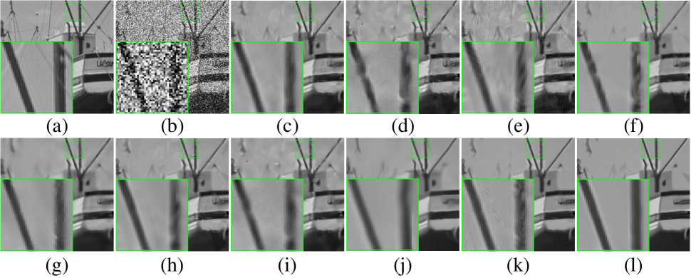
Fig. 4: Denoising results on image boats by different methods (noise level $\sigma_{n}$=75). (a) Original image; (b) Noisy image; (c) BM3D [9] (PSNR=24.82dB); (d) EPLL [34] (PSNR=24.33dB); (e) Plow [35] (PSNR=24.23dB); (f) NCSR [30] (PSNR=24.44dB); (g) PID [36] (PSNR=24.51dB); (h) PGPD [22] (PSNR=24.83dB); (i) aGMM [37] (PSNR= 24.51dB); (j) LINC [38] (PSNR= 24.44dB); (k) AST-NLS [39] (PSNR= 24.76dB); (l) GSR-NLS (PSNR=24.94dB).

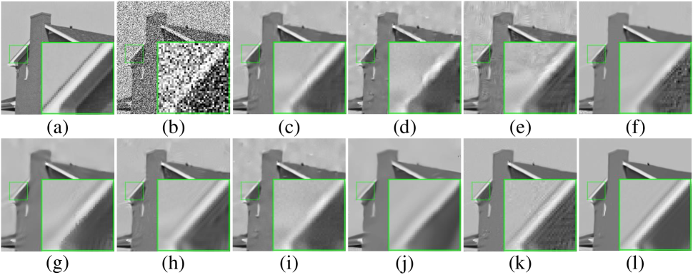
Fig. 5: Denoising results on image House by different methods (noise level $\sigma_{n}$=75). (a) Original image; (b) Noisy image; (c) BM3D [9] (PSNR=27.51dB); (d) EPLL [34] (PSNR=26.70dB); (e) Plow [35] (PSNR=26.52dB); (f) NCSR [30] (PSNR=27.16dB); (g) PID [36] (PSNR=27.35dB); (h) PGPD [22] (PSNR=27.81dB); (i) aGMM [37] (PSNR= 27.11dB); (j) LINC [38] (PSNR= 27.56dB); (k) AST-NLS [39] (PSNR= 28.06dB); (l) GSR-NLS (PSNR=28.59dB).

5 Conclusion

This paper has proposed a new method for image denoising using group sparsity residual scheme with nonlocal samples. We obtained a good estimation of the group sparse coefficients of the original image from the image nonlocal self-similarity and used it in the group sparsity residual model. An effective iterative shrinkage algorithm has been developed to solve the proposed GSR-NLS model. Experimental results have demonstrated that the proposed GSR-NLS not only outperforms many state-of-the-art methods, but also leads to a competitive speed.

References

- [1] Rudin L I, Osher S, Fatemi E. Nonlinear total variation based noise removal algorithms[J]. Physica D: nonlinear phenomena, 1992, 60(1-4): 259-268.
- [2] Osher S, Burger M, Goldfarb D, et al. An iterative regularization method for total variation-based image restoration[J]. Multiscale Modeling & Simulation, 2005, 4(2): 460-489.
- [3] Chang S G, Yu B, Vetterli M. Adaptive wavelet thresholding for image denoising and compression[J]. IEEE transactions on image processing, 2000, 9(9): 1532-1546.
- [4] Portilla J, Strela V, Wainwright M J, et al. Image denoising using scale mixtures of Gaussians in the wavelet domain[J]. IEEE Transactions on Image processing, 2003, 12(11): 1338-1351.
- [5] Wen B, Ravishankar S, Bresler Y. Structured overcomplete sparsifying transform learning with convergence guarantees and applications[J]. International Journal of Computer Vision, 2015, 114(2-3): 137-167.
- [6] Elad M, Aharon M. Image denoising via sparse and redundant representations over learned dictionaries[J]. IEEE Transactions on Image processing, 2006, 15(12): 3736-3745.
- [7] Aharon M, Elad M, Bruckstein A. -SVD: An algorithm for designing overcomplete dictionaries for sparse representation[J]. IEEE Transactions on signal processing, 2006, 54(11): 4311-4322.
- [8] Buades A, Coll B, Morel J M. A non-local algorithm for image denoising[C]//Computer Vision and Pattern Recognition, 2005. CVPR 2005. IEEE Computer Society Conference on. IEEE, 2005, 2: 60-65.
- [9] Dabov K, Foi A, Katkovnik V, et al. Image denoising by sparse 3-D transform-domain collaborative filtering[J]. IEEE Transactions on image processing, 2007, 16(8): 2080-2095.
- [10] Zhang K, Zuo W, Chen Y, et al. Beyond a gaussian denoiser: Residual learning of deep cnn for image denoising[J]. IEEE Transactions on Image Processing, 2017, 26(7): 3142-3155.
- [11] Chen Y, Pock T. Trainable nonlinear reaction diffusion: A flexible framework for fast and effective image restoration[J]. IEEE transactions on pattern analysis and machine intelligence, 2017, 39(6): 1256-1272.
- [12] Wen B, Li Y, Pfister L, et al. Joint adaptive sparsity and low-rankness on the fly: an online tensor reconstruction scheme for video denoising[C]//IEEE International Conference on Computer Vision (ICCV). 2017.
- [13] Jiang Z, Lin Z, Davis L S. Label consistent K-SVD: Learning a discriminative dictionary for recognition[J]. IEEE transactions on pattern analysis and machine intelligence, 2013, 35(11): 2651-2664.
- [14] Lun D P K. Robust fringe projection profilometry via sparse representation[J]. IEEE Transactions on Image Processing, 2016, 25(4): 1726-1739.
- [15] Dong W, Zhang L, Shi G, et al. Image deblurring and super-resolution by adaptive sparse domain selection and adaptive regularization[J]. IEEE Transactions on Image Processing, 2011, 20(7): 1838-1857.
- [16] Zha Z, Liu X, Zhang X, et al. Compressed sensing image reconstruction via adaptive sparse nonlocal regularization[J]. The Visual Computer, 2018, 34(1): 117-137.
- [17] Zhang J, Zhao D, Gao W. Group-based sparse representation for image restoration[J]. IEEE Transactions on Image Processing, 2014, 23(8): 3336-3351.
- [18] Dong W, Shi G, Ma Y, et al. Image restoration via simultaneous sparse coding: Where structured sparsity meets gaussian scale mixture[J]. International Journal of Computer Vision, 2015, 114(2-3): 217-232.
- [19] Wen B, Li Y, Bresler Y. When sparsity meets low-rankness: Transform learning with non-local low-rank constraint for image restoration[C]//Acoustics, Speech and Signal Processing (ICASSP), 2017 IEEE International Conference on. IEEE, 2017: 2297-2301.
- [20] Gu S, Zhang L, Zuo W, et al. Weighted nuclear norm minimization with application to image denoising[C]//Proceedings of the IEEE Conference on Computer Vision and Pattern Recognition. 2014: 2862-2869.
- [21] Zha Z, Liu X, Huang X, et al. Analyzing the group sparsity based on the rank minimization methods[C]//Multimedia and Expo (ICME), 2017 IEEE International Conference on. IEEE, 2017: 883-888.
- [22] Xu J, Zhang L, Zuo W, et al. Patch group based nonlocal self-similarity prior learning for image denoising[C]//Proceedings of the IEEE international conference on computer vision. 2015: 244-252.
- [23] Mairal J, Bach F, Ponce J, et al. Non-local sparse models for image restoration[C]//Computer Vision, 2009 IEEE 12th International Conference on. IEEE, 2009: 2272-2279.
- [24] Zhang L, Dong W, Zhang D, et al. Two-stage image denoising by principal component analysis with local pixel grouping[J]. Pattern Recognition, 2010, 43(4): 1531-1549.
- [25] Eldar Y C, Kuppinger P, Bolcskei H. Block-sparse signals: Uncertainty relations and efficient recovery[J]. IEEE Transactions on Signal Processing, 2010, 58(6): 3042-3054.
- [26] Li Y, Dong W, Shi G, et al. Learning parametric distributions for image super-resolution: where patch matching meets sparse coding[C]//Proceedings of the IEEE International Conference on Computer Vision. 2015: 450-458.
- [27] Yue H, Sun X, Yang J, et al. Image denoising by exploring external and internal correlations[J]. IEEE Transactions on Image Processing, 2015, 24(6): 1967-1982.
- [28] Buades A, Coll B, Morel J M. A review of image denoising algorithms, with a new one[J]. Multiscale Modeling & Simulation, 2005, 4(2): 490-530.
- [29] Daubechies I, Defrise M, De Mol C. An iterative thresholding algorithm for linear inverse problems with a sparsity constraint[J]. Communications on pure and applied mathematics, 2004, 57(11): 1413-1457.
- [30] Dong W, Zhang L, Shi G, et al. Nonlocally centralized sparse representation for image restoration[J]. IEEE Transactions on Image Processing, 2013, 22(4): 1620-1630.
- [31] Zha Z, Liu X, Zhou Z, et al. Image denoising via group sparsity residual constraint[C]//Acoustics, Speech and Signal Processing (ICASSP), 2017 IEEE International Conference on. IEEE, 2017: 1787-1791.
- [32] Z. Zha, X. Zhang, Q. Wang, Y. Bai and L. Tang, ”Image denoising using group sparsity residual and external nonlocal self-similarity prior,” 2017 IEEE International Conference on Image Processing (ICIP), Beijing, 2017, pp. 2956-2960.
- [33] Dong W, Shi G, Li X. Nonlocal image restoration with bilateral variance estimation: a low-rank approach[J]. IEEE transactions on image processing, 2013, 22(2): 700-711.
- [34] Zoran D, Weiss Y. From learning models of natural image patches to whole image restoration[C]//Computer Vision (ICCV), 2011 IEEE International Conference on. IEEE, 2011: 479-486.
- [35] Chatterjee P, Milanfar P. Patch-based near-optimal image denoising[J]. IEEE Transactions on Image Processing, 2012, 21(4): 1635-1649.
- [36] Knaus C, Zwicker M. Progressive image denoising[J]. IEEE transactions on image processing, 2014, 23(7): 3114-3125.
- [37] Luo E, Chan S H, Nguyen T Q. Adaptive image denoising by mixture adaptation[J]. IEEE transactions on image processing, 2016, 25(10): 4489-4503.
- [38] Niknejad M, Rabbani H, Babaie-Zadeh M. Image restoration using Gaussian mixture models with spatially constrained patch clustering[J]. IEEE Transactions on Image Processing, 2015, 24(11): 3624-3636.
- [39] Liu H, Xiong R, Zhang J, et al. Image denoising via adaptive soft-thresholding based on non-local samples[C]//Proceedings of the IEEE Conference on Computer Vision and Pattern Recognition. 2015: 484-492.
- [40] Yuan X, Rao V, Han S, et al. Hierarchical infinite divisibility for multiscale shrinkage[J]. IEEE Transactions on Signal Processing, 2014, 62(17): 4363-4374.