Charge transfer excitations with range separated functionals using improved virtual orbitals

Abstract

We present an implementation of range separated functionals utilizing the Slater-function on grids in real space in the projector augmented waves method. The screened Poisson equation is solved to evaluate the necessary screened exchange integrals on Cartesian grids. The implementation is verified against existing literature and applied to the description of charge transfer excitations. We find very slow convergence for calculations within linear response time-dependent density functional theory and unoccupied orbitals of the canonical Fock operator. Convergence can be severely improved by using Huzinaga’s virtual orbitals instead. This combination furthermore enables an accurate determination of long-range charge transfer excitations by means of ground-state calculations.

I Introduction

The study of intra-molecular charge transfer excitations (CTE) is of interest in photovoltaicsSariciftci et al. (1992), organic electronicsSamorí et al. (2002) and molecular and organic magnetismBlundell and Pratt (2004). Within a single particle picture, the simplest CTE is the excitation of an electron from the highest molecular orbital (HOMO) of a donor to the lowest unoccupied orbital (LUMO) of a distant acceptor. Denoting the distance between donor and acceptor by $R$, Mulliken derived the energetics of this process in the asymptote of large distances $R$ to (atomic units are used throughout)

$$E_{\text{CTE}}\approx\text{IP}_{D}-\text{EA}_{A}-\frac{1}{R},$$ (1)

where $\text{IP}_{D}$ is the ionization potential of the donor, $\text{EA}_{A}$ the electron affinity of the acceptor and $\frac{1}{R}$ approximates the Coulomb energy between the excited electron and the hole it left behindMulliken and Person (1969).

Density functional theory (DFT)Hohenberg and Kohn (1964) in the formulation of Kohn and ShamKohn and Sham (1965) is the method of choice for ab initio calculations of electronic properties of condensed matter due to its advantageous cost to accuracy ratio. In contrast to wave-function based methods, DFT expresses the total energy of a given system as functional of the electron density $n$. Although DFT is exact in principle, the exact form of this functional itself is unknown and has to be approximated in practiceLivshits and Baer (2007); Chai and Head-Gordon (2008); Cohen et al. (2008). In Kohn-Sham (KS) DFT the density is build from occupied non-interacting single-particle orbitals $\psi_{i}$ via $n=\sum_{i}f_{i}|\psi_{i}|^{2}$, where $f_{i}$ denotes the occupation number. The total energy is expressed as a sum of density functionals for the different contributions

$$E_{\text{tot}}[n]=T_{\text{S}}[n]+V_{\text{ext}}[n]+U_{\text{H}}[n]+E_{\text{xc}}[n],$$ (2)

where the $T_{\text{S}}$ denotes the kinetic energy of the non-interacting system, $V_{\text{ext}}$ the energy of the density in the external potential and $U_{\text{H}}$ the classical Coulomb energy of the density with itself. These quantities can be calculated exactly. All other energy contributions are collected in the exchange-correlation energy $E_{\text{xc}}$ which is approximated. Within a generalized KS schemeBaer et al. (2010) $E_{\text{xc}}$ can be further split into the contributions from exchange as in Hartree-Fock theory (HFT)

$$E_{\text{x}}=-\frac{1}{2}\int\int\frac{\left|\sum_{i}f_{i}\psi_{i}^{\ast}(\vec{r}_{1})\psi_{i}(\vec{r}_{2})\right|^{2}}{|\vec{r}_{1}-\vec{r}_{2}|}\text{d}\vec{r}_{1}\text{d}\vec{r}_{2},$$ (3)

and correlation $E_{\text{c}}$ that contains all energy contributions missing in the other termsKohn and Sham (1965).

Several types of approximations for $E_{\text{xc}}$ are in use. The local (LDA)Vosko et al. (1980); Perdew and Zunger (1981); Perdew and Wang (1992) functional approximates $E_{\text{xc}}$ by the local values of the density, while semi-local GGAGill (1996); Perdew et al. (1996) take local density gradients and MGGAAdamo et al. (2000); Tao et al. (2003) local values of the kinetic electron density into account (we will call local and semi-local functionals as local functionals for brevity in the following). The accuracy of local functionals is sometimes improved by hybrid functionals that combine the exchange from local functionals with the “exact” exchange integrals from HFT eq. (3) by a fixed ratioBecke (1993). While these approximations work fairly well for equilibrium propertiesBaer and Neuhauser (2005); Cohen et al. (2008), local functionals as well as hybrids fail badly in the description of CTEs because of their missing ability to describe non-local interactions correctly Dreuw et al. (2003); Baerends et al. (2013); Kümmel (2017); Maitra (2017).

Range separated functionals (RSF), that combine the exchange from the local functionals with the non-local exchange from HFT based on the spatial distance between two points $\vec{r}_{1}$ and $\vec{r}_{2}$ are able to predict the energetics and oscillator strengths of CTEs by linear response time-dependent DFT (lrTDDFT)Tawada et al. (2004); Livshits and Baer (2007); Chai and Head-Gordon (2008); Akinaga and Ten-No (2009); Rohrdanz et al. (2009); Stein et al. (2009a, b); Baer et al. (2010); Kronik et al. (2012); Zhang et al. (2012).

RSF use a separation function $\omega_{\text{RSF}}$ to split the Coulomb interaction kernel of the exchange integral (3) into two partsYanai et al. (2004)

$$\frac{1}{r_{12}}= \underbrace{\frac{1-\left[\alpha+\beta\left(1-\omega_{\text{RSF}}(\gamma,r_{12})\right)\right]}{r_{12}}}_{\text{SR, DFT}}$$

$$+\underbrace{\frac{\alpha+\beta\left(1-\omega_{\text{RSF}}(\gamma,r_{12})\right)}{r_{12}},}_{\text{LR, HFT}}$$ (4)

where $\gamma$ is a separation parameter, and $\alpha$ and $\beta$ are mixing parameters for spatially fixed and range separated mixing, respectively. The exchange from the local functionals is usually used in the short-range (SR) part, while non-local exchange integrals from HFT are used for long-range (LR) exchange. There also exists a class of RSF that uses exact exchange at short-range and the exchange from a local functional for the long-range part and is very popular for the description of periodic systemsHeyd et al. (2003, 2006), which is not the topic of our investigations, however. The correlation energy $E_{\text{c}}$ is approximated by a local functional globallyIikura et al. (2001) .

The unoccupied states entering lrTDDFT using the canonical Fock operator of HFT approximate (exited) EAsStein et al. (2010); Kronik et al. (2012). Coulomb-repulsion and exchange interaction cancel for occupied states making them subject to the interaction with $N-1$ electrons in an $N$ electron system. This cancellation is absent for unoccupied (virtual) states, making them subject to the interaction with all $N$ electrons. Therefore these unoccupied states are rather inappropriate for neutral excited state calculations.

The canonical Fock operator of HFT is not the only possible choice for the calculation of unoccupied states, as any Hermitian rotation within the space of virtual orbitals is allowedHuzinaga and Arnau (1970). Therefore it is possible to create so called improved virtual orbitals (IVOs) that are able to approximate certain excitations already at the single particle level rather accuratelyKelly (1963, 1964); Huzinaga and Arnau (1970, 1971) and we will show that these orbitals are also well suited for the calculation of charge transfer excitations within RSF.

This work is organized as follows: The following section describes the numerical methods applied and section III details the implementation of RSF in real space grids within the projector agmented wave method. Sec. IV presents the verification of our implementation against existing literature and sec. V applies RSF and its combination with IVOs to obtain CTE energies. The manuscript finally ends with conclusions.

II Methods

DFT using the real space grid implementation of the projector augmented waves (PAW)Blöchl (1994) in the GPAW packageMortensen et al. (2005); Enkovaara et al. (2010) was used for all calculations performed in this work. PAW is an all-electron method, which has shown to provide very similar results as converged basis sets for a test set of small moleculesKresse and Joubert (1999) and transition metalsValiev et al. (2003); Würdemann et al. (2015). With the exception of transition metals, where $3s$, $3p$, $3d$ and $4s$ shells were treated as valence electrons, all closed shells were subject to the frozen core approximation and (half-)open shells were treated as valence electrons. Relativistic effects were applied to the closed shells in the frozen cores in the scalar-relativistic approximation of Koelling and HarmonKoelling and Harmon (1977). If not stated otherwise, a grid-spacing of $h=0.18\,\mathrm{\text{\AA}}$ was used for the smooth KS wave function and a simulation box which contains at least $6\,\mathrm{\text{\AA}}$ space around each atom was applied. Non-periodic boundary conditions were applied in all three directions and all calculations were done spin-polarized. Only collinear spin alignments were considered. The exchange correlation functionals PBEPerdew et al. (1996), the hybrid PBE0Adamo and Barone (1998) and the RSFs LCY-BLYPAkinaga and Ten-no (2008), LCY-PBESeth and Ziegler (2012) and CAMY-B3LYPAkinaga and Ten-no (2008) were used. Linear response time-dependent density functional theory (lrTDDFT)Casida (2009); Walter et al. (2008) for RSF was implemented along the work of Tawada et al.Tawada et al. (2004) and Akinaga and Ten-NoAkinaga and Ten-No (2009). Twelve unoccupied bands were used in the lrTDDFT calculations unless stated otherwise.

III Implementation of RSF

Two functions are frequently used as separation function (4) in literature. One is the complementary error-functionIikura et al. (2001); Tawada et al. (2004); Yanai et al. (2004); Baer et al. (2006); Peach et al. (2006); Vydrov et al. (2007); Chai and Head-Gordon (2008); Rohrdanz and Herbert (2008); Wong et al. (2009) $\omega_{\text{RSF}}(\gamma,r_{12})=\operatorname{erfc}(\gamma r_{12})$ that enables efficient evaluation when the KS orbitals are represented by Gaussian functions, and the other is the Slater-functionBaer et al. (2006); Akinaga and Ten-no (2008); Akinaga and Ten-No (2009); Seth and Ziegler (2012)

$$\omega_{\text{RSF}}(\gamma,r_{12}) =e^{-\gamma r_{12}}.$$ (5)

which we will apply in our work. The Slater-function is the natural choice for a screened Coulomb potential, as it leads to the Yukawa potentialYukawa (1935) that can be derived to be the effective one-electron potential in many-electron systemsSeth and Ziegler (2012). Calculations utilizing the Slater-function were found to give superior results for the calculation of charge transfer and Rydberg excitations compared to the use of the complementary error-function Akinaga and Ten-no (2008); Akinaga and Ten-No (2009).

The calculation of the exact exchange in a RSF is straightforward in principle. Regarding only the long-range part in eq. (4) and setting $\alpha=0$ and $\beta=1$ for brevity, we have to evaluate the exchange integral

$$K^{\text{RSF}}_{ij} =\left(ij|1-\omega_{\text{RSF}}\left(\gamma,r_{12}\right)|ji\right)$$ (6)

where a Mulliken-like notation

$$\left(ij|\hat{x}|ji\right) =$$

$$\int\int \frac{\psi_{i}^{\ast}(\vec{r}_{1})\psi_{j}(\vec{r}_{1})\,\hat{x}\,\psi_{j}^{\ast}(\vec{r}_{2})\psi_{i}(\vec{r}_{2})}{|\vec{r}_{1}-\vec{r}_{2}|}\,\text{d}\vec{r}_{1}\text{d}\vec{r}_{2}$$ (7)

with the one-particle functions $\psi_{i,j}$ and the operator $\hat{x}$ is used. The first part of eq. (6) is the standard exchange integral $K_{ij}=\left(ij|ji\right)$ from HFTRostgaard (2006); Enkovaara et al. (2010) and the additional term is the screened exchange integral

$$K^{\gamma}_{ij} =\left(ij|\omega_{\text{RSF}}\left(r_{12}\right)|ji\right)\;.$$ (8)

In PAW the KS wave-function (WF) $\psi_{i}$ is represented as a combination of a soft pseudo WF, $\tilde{\psi}_{i}$ and atom-centered (local) correctionsBlöchl (1994); Mortensen et al. (2005); Enkovaara et al. (2010)

$$\psi_{i} =\tilde{\psi}_{i}+\sum_{\alpha}\sum_{k}\left(|\phi_{k}^{\alpha}\rangle-|\tilde{\phi}_{k}^{\alpha}\rangle\right)\mathcal{P}_{ik}^{\alpha},$$ (9)

where $\phi_{k}^{\alpha}$ and $\tilde{\phi}_{k}^{\alpha}$ denote atom centered all-electron and soft partial WFs, respectively, and $\mathcal{P}_{ik}^{\alpha}$ is a projection operator which maps the pseudo WF on the partial WF. The all-electron and soft partial WF match outside of the atom centered augmentation sphere. The band-indices $i$ and $k$ contain the main quantum numbers and $\alpha$ is the atomic index which runs over all atoms in the calculation.

In our implementation, the pseudo WFs are evaluated on three dimensional Cartesian grids in real space while the partial WFs are evaluated on radial gridsMortensen et al. (2005); Enkovaara et al. (2010). Using the exchange density $n_{ij}=\psi_{i}^{\ast}\psi_{j}$ and the local exchange density $n^{\alpha}_{ij}=\sum_{k_{1}k_{2}}\phi_{k_{1}}^{\alpha}\phi_{k_{2}}^{\alpha}\mathcal{P}_{ik_{1}}^{\alpha\ast}\mathcal{P}_{jk_{2}}^{\alpha}$ the integral (8) can be written as

$$\left(\left(n_{ij}\right)\right)^{\gamma} =\left(\left(\tilde{n}_{ij}\right)\right)^{\gamma}+\sum_{\alpha}\left[\left(\left(n^{\alpha}_{ij}\right)\right)^{\gamma}-\left(\left(\tilde{n}^{\alpha}_{ij}\right)\right)^{\gamma}\right],$$ (10)

where

$$\left(\left(n_{ij}\right)\right)^{\gamma}=\left(n_{ij}|n_{ji}\right)^{\gamma}=\left(n_{ij}|\exp\left(-\gamma r_{12}\right)|n_{ji}\right)$$

is used as shortcut for the screened exchange interaction of the exchange density with itself. Due to the non-locality of the screened exchange operator, a straight application of eq. (10) would lead to cross-terms between local functions located on different atomic sites and the need to integrate on incompatible gridsBlöchl (1994); Mortensen et al. (2005). To avoid these, compensation charges $\tilde{Z}_{ij}^{\alpha}$ are introducedRostgaard (2006); Enkovaara et al. (2010) such that using $\tilde{\varrho}_{ij}=\tilde{n}_{ij}+\sum_{\alpha}\tilde{Z}_{ij}^{\alpha}$ allows to write

$$\left(\left(n_{ij}\right)\right)^{\gamma} =\left(\left(\tilde{\varrho}_{ij}\right)\right)^{\gamma}+\sum_{\alpha}\Delta K_{ij}^{\alpha\gamma},$$ (11)

where $\left(\left(\tilde{\varrho}_{ij}\right)\right)^{\gamma}$ is free of local contributions. The evaluation of the $\Delta K_{ij}^{\alpha\gamma}$ using the integration kernel from Rico et al.Rico et al. (2012) is detailed in supporting information (SI).

Direct evaluation of the double-integral

$$I =\int\int\tilde{\varrho}_{ij}(1)\frac{e^{-\gamma r_{12}}}{r_{12}}\tilde{\varrho}_{ji}(2)\text{d}\vec{r}_{1}\text{d}\vec{r}_{2}$$ (12)

on a three dimensional Cartesian grid is not only time-consuming, but also suffers from the singularity at $\vec{r}_{1}=\vec{r}_{2}$. To circumvent this, the integral is solved using the method of the Green’s functions

$$I =\int\tilde{\varrho}_{ij}(\vec{r}_{1})\tilde{v}_{ji}(\vec{r_{1}})d\vec{r}_{1}\;.$$ (13)

The potential $\tilde{v}_{ij}$ is calculated by solving the screened Poisson or modified Helmholtz equationJackson (1998); Greengard and Huang (2002)

$$\left(\nabla^{2}-\gamma^{2}\right)\tilde{v}_{ij}(\vec{r_{1}}) =-4\pi\tilde{\varrho}_{ij}(\vec{r_{1}})\;.$$ (14)

A finite difference scheme together with a root finderMortensen et al. (2005); Enkovaara et al. (2010) is chosen, where a constant representing $\gamma$ is added to the central point of the finite difference stencilWajid et al. (2014). The potential $\tilde{v}_{ij}$ of a charge system decays very slowly and the (screened) Poisson equation (14) is therefore applied for neutral charge distributions onlyEnkovaara et al. (2010). Charged systems are neutralized by subtracting a Gaussian density for which the solution is known analytically (see SI for details).

Range separated functionals also contain a contribution of the density functional exchange. Akinaga and Ten-no derived an analytic expression for the exchange contribution of a GGA in the case of a Slater-function based RSF, $E_{\text{x}}^{\text{GGA}}\left(\gamma\right)$Akinaga and Ten-no (2008). Seth and Ziegler discovered, that this expression leads to numerical instabilities for very small densities and derived a superior expression for small densities based on a power series expansionSeth and Ziegler (2012). Both expressions along with analytic expressions for the first, second, and third derivatives of $E_{\text{x}}^{\text{GGA}}(\gamma)$ based on the analytic expression derived by Akinaga and Ten-no were implemented in libxcMarques et al. (2012); Lehtola et al. (2018).

IV Verification of the implementation

		TiO2			CuCl			CrO3
Functional	$\gamma$	ours	lit.	$\text{d}E$	ours	lit.	$\text{d}E$	ours	lit.	$\text{d}E$
PBE		$7.56$	$7.53^{a}$	$0.03$	$3.74$	$3.73^{a}$	$0.01$	$5.67$	$5.66^{a}$	$0.01$
PBE		–"–	$7.56^{b}$	$0.00$	–"–	$3.67^{b}$	$0.07$	–"–	$6.07^{b}$	$-0.4$
PBE0		$6.45$	$6.44^{a}$	$0.01$	$3.54$	$3.62^{a}$	$-0.08$	$4.24$	$4.28^{a}$	$-0.04$
PBE0		–"–	$6.47^{b}$	$-0.02$	–"–	$3.50^{b}$	$0.04$	–"–	$4.63^{b}$	$-0.39$
LCY-BLYP	$0.70$	$6.24$	$6.33^{b}$	$-0.09$	$3.44$	$3.69^{b}$	$-0.25$	$4.16$	$4.75^{b}$	$-0.59$
	$0.75$	$6.12$	$6.21^{b}$	$-0.09$	$3.43$	$3.68^{b}$	$-0.25$	$4.01$	$4.59^{b}$	$-0.58$
LCY-PBE	$0.75$	$6.38$	$6.47^{b}$	$-0.09$	$3.63$	$3.88^{b}$	$-0.25$	$3.93$	$4.74^{b}$	$-0.81$
	$0.90$	$6.04$	$6.14^{b}$	$-0.10$	$3.60$	$3.84^{b}$	$-0.24$	$3.49$	$4.29^{b}$	$-0.8$
CAMY-B3LYP	$0.34$	$6.32$	$6.38^{b}$	$-0.06$	$3.32$	$3.43^{b}$	$-0.11$	$4.34$	$4.89^{b}$	$-0.55$
$\overline{\text{d}E}_{\text{RSF}}$				$-0.09$			$-0.22$			$-0.67$
exp.			$6.62^{c}$			$3.81^{c}$			$4.97^{c}$

Table 1: Mean ligand removal enthalpies (see text) for TiO₂, CuCl, and CrO₃ from our calculations compared to the literature. $dE$ denotes the difference between our results and the literature values. Geometries were taken from Johnson and BeckeJohnson and Becke (2009) and energies are given in $\mathrm{eV}$. References and basis-sets: ^a6–311++G(3df,3pd) ref. 65, ^bTZ2P ref. 49, ^cexperiment ref. 66.

A large amount of work was devoted to RSF in the literatureIikura et al. (2001); Tawada et al. (2004); Toulouse et al. (2004); Yanai et al. (2004); Baer and Neuhauser (2005); Baer et al. (2006); Peach et al. (2006); Vydrov and Scuseria (2006); Vydrov et al. (2006); Cohen et al. (2007); Livshits and Baer (2007); Gerber et al. (2007); Vydrov et al. (2007); Akinaga and Ten-no (2008); Chai and Head-Gordon (2008); Henderson et al. (2008); Livshits and Baer (2008); Rohrdanz and Herbert (2008); Akinaga and Ten-No (2009); Livshits et al. (2009); Rohrdanz et al. (2009); Stein et al. (2009b, a); Wong et al. (2009); Baer et al. (2010); Stein et al. (2010); Refaely-Abramson et al. (2011); Kronik et al. (2012); Seth and Ziegler (2012); Zhang et al. (2012); Seth et al. (2013); Autschbach and Srebro (2014); Cabral do Couto et al. (2015). In order to verify our implementation, we have re-calculated some of the published properties in our grid-based approach. Seth and ZieglerSeth and Ziegler (2012) calculated the mean ligand removal enthalpies defined asJohnson and Becke (2009); Seth and Ziegler (2012)

$$\bar{E}_{L} =\frac{nE(L)+mE(M)-E(M_{m}L_{n})}{n+m-1}$$ (15)

for a group of molecules including transition metals. We have calculated this quantity for the molecules TiO₂, CuCl, and CrO₃ and compared our results against the values published by Johnson and BeckeJohnson and Becke (2009) for PBE and PBE0, as well as Seth and ZieglerSeth and Ziegler (2012) for PBE, PBE0 and a group of RSF in tab. 1. As the literature values were calculated without relativistic corrections, we have neglected relativistic effects in the reported values also. A grid spacing of $h=0.16\,\mathrm{\text{\AA}}$ was necessary to correctly describe $3d$-splittingWürdemann et al. (2015) (see SI for details).

Generally, our PBE and PBE0 values are in good agreement to the results obtained from both groups for TiO₂ and CuCl. There is a difference of about $0.4\,\mathrm{eV}$ to the work of Seth and Ziegler for CrO₃, while our values are a in good agreement to the work of Johnson and Becke. These differences can attributed the different basis sets used. While Johnson and Becke used the rather large 6–311++G(3df,3pd) basis set, Seth and Ziegler use a smaller TZ2P basis set that is apparently not large enough. We have observed similar strong basis set effects in particular if chromium is involved already in prior studies for chromiumWürdemann et al. (2015).

RSF results using Slater functions are unfortunately only available from the TZ2P basis set. While our results are in good agreement to Seth and Ziegler for TiO₂ ($\leq-0.09\,\mathrm{eV}$ deviation), they already differ by up to $0.25\,\mathrm{eV}$ for CuCl. CAMY-B3LYP, which includes only a fraction of the screened exchange, generally leads to the smallest deviations. RSFs are obviously very sensitive to basis set limitations due to the long range of the effective single particle potentialBaer et al. (2010). We therefore trust the values obtained by our method which represent the large basis set limit.

In comparison to experiment, PBE ligand removal energies are rather accurate for CuCl, but this functional over-binds TiO₂ and CrO₃. In the latter molecules $d$-orbitals contribute to binding and might be responsible for this overbinding. In contrast, the hybrid PBE0 as well as the RSFs tend to underbind in all three molecules, in particular if $d$-orbitals are involved. Interestingly, this trend is similar to the overestimation of $d$-binding in PBE and the lack of proper $d$-binding by hybrids we have observed in the Cr-dimer beforeWürdemann et al. (2015).

The value of the separation parameter $\gamma$ can not be defined rigorously and its optimal choice is under discussion. A system dependence is to be expectedIikura et al. (2001); Baer et al. (2006); Livshits and Baer (2007); Chai and Head-Gordon (2008); Livshits and Baer (2008); Baer et al. (2010); Stein et al. (2010); Refaely-Abramson et al. (2011); Kronik et al. (2012). The group around Roi Baer devised schemes to optimize $\gamma$ without the use of empirical parametersLivshits and Baer (2007, 2008); Stein et al. (2009a) by forcing the difference between the ionization potential (IP) calculated from total energy differences and the negative eigenvalue of the HOMO $-\epsilon_{\text{HOMO}}$ of an $N$ electron system to vanishLivshits and Baer (2007)

$$\underbrace{\left[E_{\text{gs}}\left(N,\gamma\right)-E_{\text{gs}}\left(N-1,\gamma\right)\right]}_{\text{IP}(N)}$$

$$\stackrel{{\scriptstyle\gamma=\gamma_{\text{opt}}}}{{\equiv}}-\epsilon_{\text{HOMO}}(N,\gamma)\;.$$ (16)

This condition is fulfilled for the exact functionalAlmbladh and von Barth (1985), but is usually violated by local and hybrid approximationsLivshits and Baer (2007). Livshits and Baer also devised an approach to determine $\gamma$ for the calculation of binding energy curves of symmetric bi-radical cations which imposes a match of the slopes of the energy curves for the charged and neutral moleculeLivshits and Baer (2008)

$$E_{\text{gs}}\left(N-\frac{1}{2},\gamma\right)-E_{\text{gs}}\left(N-1,\gamma\right)$$

$$\quad\stackrel{{\scriptstyle\gamma=\gamma_{\text{opt}}}}{{\equiv}}E_{\text{gs}}\left(N,\gamma\right)-E_{\text{gs}}\left(N-\frac{1}{2},\gamma\right)\;.$$ (17)

Their group found that both approaches give almost identical values of $\gamma_{\text{opt}}$ for the same systemBaer et al. (2010), which we confirm in the case of Cr₂. We will denote an RSF using an optimized value of $\gamma$ obtained by eqs. (16, 17) by appending an asterisk, e.g. LCY-PBE^∗.

	Cr		Cr2		CO		N2
	$-\epsilon_{\text{H}}$	IP	$-\epsilon_{\text{H}}$	IP	$-\epsilon_{\text{H}}$	IP	$-\epsilon_{\text{H}}$	IP
exp.Lias and Liebmann (2016)		$6.77$		$6.4$		$14.01$		$15.58$
PBE	$3.70$		$4.29$		$9.09$		$10.24$
PBE0	$4.95$				$10.79$		$12.16$
BNL∗Livshits and Baer (2007)					$14.3$		$16.6$
LCY-PBE∗	$6.79$		$6.85$		$14.32$	$14.31$	$16.33$	$16.32$
$\gamma^{\text{BNL}}_{\text{opt}}(a_{0}^{-1})$Livshits and Baer (2007)					0.6		0.6
$\gamma^{\text{LCY}}_{\text{opt}}(a_{0}^{-1})$	0.72		0.45		0.81		0.99

Table 2: Negative eigenvalue of the HOMO $-\epsilon_{\text{H}}$, IP and values of the screening parameter $\gamma$ for Cr, Cr₂, CO and N₂ calculated using different functionals. All energies given in $\mathrm{eV}$.

We used eq. (16) to obtain $\gamma_{\text{opt}}$ for Cr, Cr₂, CO and N₂ and verified that the eigenvalues for the HOMO as well as the experimental value of the ionization potential match in this case. The resulting screening parameters for the RSF BNL^* and LCY-PBE^* are listed in tab. 2. BNL^* is a LDA based RSF used by Livshits and Baer which utilizes the error-function instead of the Slater functionLivshits and Baer (2007). For the gradient corrected PBE and the hybrid-functional PBE0 the eigenvalues of the HOMO doesn’t match the experimental ionization potential. This is different for the RSF: The eigenvalues for the HOMO are in quite good, for N₂, to, in the case of Cr, perfect agreement to the experimental ionization potential. For the cases of CO and N₂ also a good agreement between the values from Livshits and Baer and this work is achieved. For the values of the screening parameter a $\gamma^{\text{LCY}}_{\text{opt}}\approx\frac{3}{2}\gamma^{\text{BNL}}_{\text{opt}}$ dependency between the used screening functions, Slater vs. error-function, was statedShimazaki and Asai (2008). The comparison between the values listed in tab. 2 supports this dependency.

		LCY-PBE*		BNL*Baer et al. (2010)
state	IPPotts and Price (1972) (eV)	Koop.	lr.	Koop.	lr.
1b1	$12.62$	1%	1%	-1%	-1%
3a1	$14.74$	0%	4%	-3%	-3%
1b2	$18.51$	0%	3%	-1%	-1%
2a1a	$32.20$	0%	4%	-1%	0%

Table 3: Deviation of the calculated IPs of H₂O calculated with LCY-PBE^∗ and using Koopmans theorem or lrTDDFT along with the experimental values and values calculated by Baer et al.Baer et al. (2010). In this work, $\gamma$ was tuned to $0.831\,\mathrm{a_{0}^{-1}}$. $a$: Ref. 10 gave $30.9\,\mathrm{eV}$ as ionization potential for the 2a₁ state. Koop.: prediction by use of Koopman’s theorem, lr.: prediction by use of $\Delta$-SCF and lrTDDT.

Baer et al. also discussed the impact of the tuning of $\gamma$ on the inner ionization energies (ionization into an excited state of the cation). They stated, that by tuning $\gamma$ one is able to predict the inner ionization energies not only by the combination of a $\Delta$SCF and lrTDDFT calculation but also directly by the density of states of the neutral molecule in the sense of Koopmans theoremKoopmans (1934) from HFTBaer et al. (2010). In this work their example, H₂O was also verified. The deviations between the calculated IPs and the experimental values are shown in tab. 3. The calculated values are in a very good agreement to each other and to experiment, despite the issue, that Baer et al. gave a ionization potential for the 2a₁ state which differs from the value used as reference in both works.

V Charge transfer excitations

In this section we investigate the description of charge transfer excitations (CTE) within RSF. One of the frequently used model systems to study CTE is the ethylene-tetrafluoroethylene dimerDreuw et al. (2003); Tawada et al. (2004); Zhao and Truhlar (2006); Peach et al. (2006); Livshits and Baer (2007); Chai and Head-Gordon (2008); Rohrdanz et al. (2009); Zhang et al. (2012). This choice is not fortunate, as both constituents exhibit a negative EAChiu et al. (1979), which leads to CTE that overlap with the continuum at least for infinite separation. Therefore we use the alternative Na₂–NaCl complex, where Na₂ is the donor and NaCl the acceptor with a positive EA (experimental adiabatic EA of 0.73 eVMiller et al. (1986)). In order to catch the largely delocalized excited states we increased the amount of space within our simulation box to $x_{\text{vac}}=11\,\mathrm{\text{\AA}}$ around each atom and decreased the grid spacing to $h=0.2\,\mathrm{\text{\AA}}$ due to the higher computational effort.

Mol.	IPexp.Lias and Liebmann (2016)	IPcalc	$-\epsilon_{\text{H}}$	$\text{d}E$
Na2	$4.892\pm 0.003$	$4.93$	$4.94$	$-0.01$
NaCl-	$0.727\pm 0.010$	$0.79$	$0.78$	$0.01$

Table 4: Experimental, IP_exp., and calculated, IP_calc, ionization potential for the molecules Na₂ and NaCl^- along with the negative eigenvalue of the HOMO $-\epsilon_{\text{H}}$ and their difference $\text{d}E={\rm IP}\textsubscript{calc}+\epsilon_{\text{H}}$. All values are in eV.

Using eq. (16) to calculate $\gamma_{\text{opt}}$ for the individual molecules leads to $\gamma_{\text{opt}}=0.38\,\mathrm{a_{0}^{-1}}$ for Na₂ and $\gamma_{\text{opt}}=0.40\,\mathrm{a_{0}^{-1}}$ for NaCl^-. In order to obtain the optimal range separation parameter for the combined system, the Na₂–NaCl complex, we use minimization of the function Stein et al. (2009a)

$$J(\gamma)= \sum_{i=D^{0},A^{-}}\Big{|}\epsilon_{\text{HOMO}}^{i}(\gamma)+\text{IP}_{i}(N,\gamma)\Big{|}$$ (18)

with $\text{IP}_{i}(N,\gamma)=E_{\text{gs}}^{i}(N_{i}-1,\gamma)-E_{\text{gs}}^{i}(N_{i},\gamma)$, where $D^{0}$ denotes the neutral donor, $A^{-}$ the acceptor anion and $N$ the number of electrons. The two molecules were considered separately where the experimental geometries of the neutral molecules from ref. 87 were used. This treatment results in a value of $\gamma_{\text{opt}}=0.39\,\mathrm{a_{0}^{-1}}$, which leads to the energies in table 4 that exhibit good agreement to experiment. The eigenvalue of the NaCl LUMO ($\epsilon_{\text{LUMO}}=-0.57\,\mathrm{eV}$) differs from the eigenvalue of the NaCl^- HOMO which equals the NaCl EA through (18) by $\approx 0.2\,\mathrm{eV}$. This effect is known and can be attributed to the derivative discontinuityStein et al. (2010); Kronik et al. (2012).

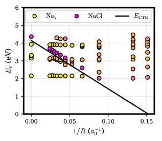
Figure 1: Linear response TDDFT excitations of the Na₂–NaCl-system depending on the inverse distance between the two molecules $\nicefrac{{1}}{{R}}$. The colors indicate localization of the unoccupied states involved in the excitations on Na₂ (yellow) or NaCl (purple). Solid line: excitation energy after eq. (1).

In order to study CT excitations, the molecules were placed with their axes parallel to each other. We first consider the singlet excited state spectrum of the donor acceptor pair calculated by linear response TDDFT depending on the molecular separation as depicted in fig. 1. The separation $R$ is given by the separation of the two parallel molecular axes. The excitations are colored by the weights of the involved unoccupied orbitals on the individual molecules. Only excitations with more than $50\,\mathrm{\%}$ contribution from the Na₂ HOMO and either an oscillator strength $\geq 10^{-2}$ or $90\,\mathrm{\%}$ weight on NaCl are considered. The excitation spectrum shows a clear CTE where the involved unoccupied states are clearly located on NaCl and its energy follows the expectation of Mullikens law eq. (1) for larger separations ($1/R\leq 0.08\leavevmode\nobreak\ a_{0}^{-1}$) as expected. There is a small constant deviation from the expectations of eq. (1) that arises from the difference between the eigenvalue of the NaCl LUMO and the NaCl EA [entering in eq. (1)]. This is validated by the NaCl point at $1/R=0$ which is placed at the energy of IP_D + $\epsilon_{\text{LUMO, NaCl}}$.

There is more interaction between the two molecules for smaller distances. Therefore the excited states start to mix and their nature is harder to identify. The excitation energies exhibit a noticeable blur even for large $R$, where little interaction between the molecules would be expected. This is particularly visible in excitations localized on the Na₂ molecule, which exhibit a large degree of delocalization, viewable by the coloring of excitations around $3\,\mathrm{eV}$.

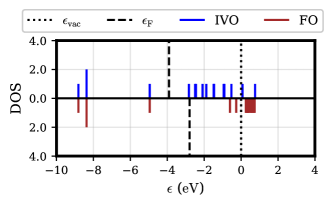
Figure 2: Density of electronic states (DOS) of the Na₂–NaCl-system at distance $8\,\mathrm{\text{\AA}}$ for the canonical Fock operator (FO) and for improved virtual orbitals (IVO). The vacuum level $\epsilon_{\text{vac}}$ is indicated and used as energy reference. The Fermi level is set to $\epsilon_{\text{F}}=\frac{\epsilon_{\text{HOMO}}+\epsilon_{\text{LUMO}}}{2}$ (all states below $\epsilon_{\text{F}}$ are occupied, all states above are unoccupied).

This numerical noise can be attributed to the fact that already the third unoccupied state in the Na₂ ground-state calculation is above the vacuum level and thus this state and all higher ones are influenced by eigenstates of the simulation box (fig. 2). This hinders the convergence of these excitations in the number of unoccupied states involved as shown below.

In HFT the Coulomb- and exchange interaction cancel for an occupied state with itself, such that these states are subject to the interaction with $N-1$ electrons in an $N$ electron system. This cancellation is absent for unoccupied (virtual) states making them subject to the interaction with all $N$ electrons. Unoccupied states therefore “see” a neutralized core in a neutral system and thus approximate (exited) EAs in HFT and not excitations of the neutral systemKoopmans (1934); Baerends et al. (2013). As many neutral closed shell molecules exhibit a negative EA Baerends et al. (2013), the eigenvalues of unoccupied states in HFT type calculations like RSF become positive, i.e. they reside in the continuum (see fig. 2). In calculations utilizing basis-sets, these states are stabilized by the finite size of the basis-setRösch and Trickey (1997); Tozer and De Proft (2005); Baerends et al. (2013) and their properties thus get strongly basis set dependent. Similarly, these states strongly couple to eigenstates of the simulation box in grid-based calculations used here. Therefore RSF DFT calculations become numerically very demanding on grids due to numerical instabilitiesWürdemann (2016).

VI Improved virtual orbitals

Improved virtual orbitals are a remedy for the difficulties mentioned above. The canonical Hartree-Fock operator is not unique in case of unoccupied orbitals in HFT. These states do not contribute to the Slater determinant built from occupied states exclusively, any set of orbitals orthogonal to the occupied states could serve as valid set of unoccupied states. Following the work of KellyKelly (1963, 1964), Huzinaga and Arnau devised a scheme to use this freedom to better approximate excitations in HFTHuzinaga and Arnau (1970, 1971). In this scheme Coulomb and exchange interactions between a virtual hole in an initial occupied orbital $k$ and the virtual orbitals are described by a modified Fock-Operator Huzinaga and Arnau (1970)

$$\hat{F}^{\text{IVO}}_{i} =\hat{F}_{i}+\hat{V}$$ (19)

$$\hat{V} =\left(1-\hat{P}\right)\hat{\Omega}_{k}\left(1-\hat{P}\right)$$ (20)

$$\hat{P} =\sum_{i}^{N}\left|\psi_{i}\rangle\langle\psi_{i}\right|.$$ (21)

$\hat{F}_{i}$ denotes the canonical Fock-Operator and $\psi_{i}$ the non-interacting single particle Hartree-Fock or, in the case of the present study, KS orbitals. $\hat{P}$ separates the space of the unoccupied orbitals from the occupied ones, circumventing slight changes in the eigenstates of the occupied states which occur otherwiseKelly (1964); Huzinaga and Arnau (1970). The rotation operator $\hat{\Omega}_{k}$ can be chosen arbitrarily as long as it is HermitianHuzinaga and Arnau (1970). Huzinaga and Arnau suggested to useHuzinaga and Arnau (1971)

$$\hat{\Omega}_{k} =-\hat{J}_{k}+\hat{K}_{k}\pm\hat{K}_{k}$$ (22)

for closed shell systems (as is the case discussed below) following the work of Hunt and Goddard IIIHunt and Goddard III (1969). $\hat{J}_{k}$ denotes the Coulomb-, $\hat{K}_{k}$ the exchange operator and $k$ the band-index of the orbital to excite from. The second exchange term can be used to approximate either singlet (“+”, $\hat{\Omega}_{k}^{\text{S}}$) and triplet (“-”, $\hat{\Omega}_{k}^{\text{T}}$) excitations, or can be omitted ($\hat{\Omega}_{k}^{\text{A}}$) to approximate their average. The initial orbital $k$ can be chosen arbitrarily Huzinaga and Arnau (1970, 1971) and determines the nature of the excitations to be described. Virtual orbitals subject to this scheme are called improved virtual orbitals (IVO) Huzinaga and Arnau (1970, 1971).

The IVO scheme (21) can also be applied within RSF setting $\hat{K}_{k}=\hat{K}_{k}^{\text{RSF}}$ as in eq. (6) and $\hat{J}_{k}=\hat{J}_{k}^{\text{RSF}}$ as the corresponding screened Coulomb counterpart. We have disregarded the orthogonalization through operator $\hat{P}$ due to numerical instabilities and $\hat{\Omega}_{k}$ was applied to the unoccupied states only. The matrix elements in the exact exchange part of the Hamiltonian mixing occupied and unoccupied states were set to zero consistently. We have verified that both approaches lead to virtually identical eigenvalues (see SI). As we will investigate the possibility of the combination of RSF and IVOs for the prediction of excitation energies by means of ground-state calculations we have used the singlet form: $\hat{\Omega}_{k}^{\text{S}}=-\hat{J}_{k}+2\hat{K}_{k}$, where $k$ is the quantum number of the HOMO located on Na₂. The resulting density of states is depicted in fig. 2. While the occupied state energies of the canonical Fock operator and the IVO operator agree by definition, the IVO operator leads to many more states below the vacuum level $\epsilon_{\text{vac}}$. There are infinitely many Rydberg states below $\epsilon_{\text{vac}}$ in principle, but these do not appear due to the finite box size in our calculations.

It was shown, that lrTDHFT excitation energies in the Tamm-Dancoff approximation and IVO Eigenenergies agree in a two-orbital two electron modelCasida and Huix-Rotllant (2012). Therefore the IVOs can be expected to represent a good basis for lrTDDFT calculations. Their use involves slight modifications of the usual formalism in the formulation of lrTDDFT as generalized eigenvalue problemDreuw et al. (2003); Casida (2009); Akinaga and Ten-No (2009)

$$\begin{pmatrix}\mathbf{A}&\mathbf{B}\\ \mathbf{B^{\ast}}&\mathbf{A^{\ast}}\end{pmatrix}\begin{pmatrix}\vec{X}\\ \vec{Y}\end{pmatrix} =\omega\begin{pmatrix}\mathbf{1}&\mathbf{0}\\ \mathbf{0}&-\mathbf{1}\end{pmatrix}\begin{pmatrix}\vec{X}\\ \vec{Y}\end{pmatrix},$$ (23)

where $\vec{X}/\vec{Y}$ denote the excitations/de-excitations, and $\mathbf{1}$ the unity-matrix. The matrix elements of $\mathbf{A}$ and $\mathbf{B}$ are given by

$$A_{ia\sigma,jb\tau} =\delta_{ij}\delta_{ab}\delta_{\sigma\tau}\left(\epsilon_{a}-\epsilon_{i}\right)+K_{ia\sigma,jb\tau}$$ (24)

$$B_{ia\sigma,jb\tau} =K_{ia\sigma,bj\tau}$$ (25)

with the $K_{ia\sigma,jb\tau}$ written in the most general form (see SI)

$$K_{ia\sigma,jb\tau} =\left(i_{\sigma}a_{\sigma}|\nicefrac{{1}}{{r_{12}}}|j_{\tau}b_{\tau}\right)$$

$$\quad+\left(1-\alpha-\beta\right)\left(i_{\sigma}a_{\sigma}|f_{\text{xc}}|j_{\tau}b_{\tau}\right)$$

$$\quad+\beta\left(i_{\sigma}a_{\sigma}|f_{\text{xc}}^{\text{RSF}}|j_{\tau}b_{\tau}\right)$$

$$\quad-\delta_{\sigma\tau}\left(ij\left|\frac{\alpha+\beta\left(1-\omega_{\text{RSF}}\right)}{r_{12}}\right|ab\right)\;.$$ (26)

Mulliken notation

$$\left(ab|\hat{x}|cd\right)=$$

$$\int\int a^{\ast}(\vec{r_{1}})b(\vec{r_{1}}) \hat{x}(\vec{r_{1}},\vec{r_{2}},...)c^{\ast}(\vec{r_{2}})d(\vec{r_{2}})\text{d}\vec{r_{1}}\text{d}\vec{r_{2}}$$

was used and $f_{\text{xc}}=\frac{\delta^{2}E_{\text{xc}}}{\delta\varrho\left(\vec{r_{1}}\right)\delta\varrho\left(\vec{r_{2}}\right)}$ is exchange-correlation kernel of the local functional and $f_{\text{xc}}^{\text{RSF}}$ the damped exchange-correlation kernel derived from $E_{\text{x}}^{\text{GGA}}(\gamma)+E_{\text{c}}^{\text{GGA}}=E_{\text{xc}}^{\text{GGA}}(\gamma)$. Occupied orbital indices are denoted by $i$ and $j$, unoccupied orbitals by $a$ and $b$, and $\sigma$ and $\tau$ are the spin-indices, while $\alpha$ and $\beta$ are the mixing parameters from the CAM scheme eq. (4). The use of IVOs requires to modify the matrix $\mathbf{A}$ toBerman and Kaldor (1979)

$$A_{ia\sigma,jb\tau}^{\text{IVO}} =A_{ia\sigma,jb\tau}$$

$$\quad+\delta_{ab}\delta_{\sigma\tau}\left[\left(aa|kk\right)-\left(ak|ka\right)\right.$$

$$\left.\quad\quad\mp\left(ak|ka\right)\right]$$

$$=A_{ia\sigma,jb\tau}-\delta_{ab}\delta_{\sigma\tau}\left\langle a\left|\hat{\Omega}_{k}\right|a\right\rangle$$ (27)

where $k$ denotes the excitation orbital and $\hat{\Omega}_{k}$ is defined in (22). The matrix $\mathbf{B}$ remains the same.

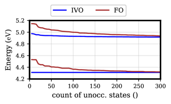
Figure 3: Convergence of the two lowest singlet excitation energies of the isolated NaCl molecule using the canonical Fock operator (FO) and improved virtual orbitals (IVO).

The use of IVO indeed facilitates the calculation of excitations using lrTDDFT as shown in fig. 3 for the two first singlet excitations of the isolated NaCl molecule. These are excitations mainly from the degenerated HOMO and HOMO-1 to the LUMO and converge rapidly in the IVO basis. In contrast, more than 200 unoccupied orbitals of the canonical HF operator are needed to arrive at converged energies, which shows that this basis is not very appropriate for the description of excitations. It is known, that excitations calculated by linear response time dependent HFT need a large linear combination of single particle excitations (i.e. a high number of unoccupied states), while excitations calculated by lrTDDFT using the kernels of local functionals can often be described by an individual excitationvan Meer et al. (2014, 2017). The twelve unoccupied states that are used in the lrTDDFT calculations for the Na₂–NaCl-system presented in fig. 1 utilizing the canonical FO are therefore far from converged for the neutral excitations. This is seen by the CTE state and the first excitation of Na₂ in fig. 1, which are rather clear as these only involve states with negative eigenvalues which do not couple with the eigenstates of the simulation box.

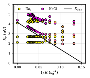
Figure 4: Linear response TDDFT excitations of the Na₂–NaCl-system depending on the inverse distance between the two molecules $\nicefrac{{1}}{{R}}$ as in fig. 1 using IVOs with $\hat{\Omega}_{k}^{S}$ and $k$ was chosen as the HOMO of the Na₂ molecule. Besides the use of the IVOs, everything like fig. 1.

The IVOs provide a better basis for the calculation of excitations as can be seen in the lrTDDFT spectrum for the Na₂–NaCl system utilizing IVOs depicted in fig. 4. The depicted states are selected and colored as in fig. 1. The “hole” is in the HOMO of the Na₂ molecule. The spectrum gets much clearer than in fig. 1 and the energy of the second excitation on Na₂ is clearly lower and it is strongly localized on Na₂ due to better convergence. Again, the calculated CTE energies are in perfect agreement to the behavior predicted by Mullikens law eq. (1), except the offset due to the difference between the eigenvalue of the NaCl LUMO and its calculated EA. A second CTE state approximately $1\,\mathrm{eV}$ above the first can be identified. which is not the case in fig. 1. This is an effect of the stronger stabilization due to the artificial hole.

This suggests that RSFs might be also used to calculate the energetics of CTEs by means of ground-state calculations within the IVO formalism. This conjecture can be further rationalized in particular for CTEs, where HOMO and LUMO are spatially strongly separated such that most of the weight in eq. (4) resides on the exchange integrals from HFT. By adding $\hat{V}$ from eq. (20) to the Kohn-Sham-Hamiltonian and taking the HOMO as the hole-state $k$, the eigenvalue of the LUMO in a RSF becomes $\epsilon_{\text{LUMO}}\approx-\text{EA}_{A}^{\text{calc}}-\hat{J}_{k}$, where it was used that the HOMO and LUMO orbitals do not overlap which leads to vanishing exchange ($\hat{K}_{k}\to 0$). With $\epsilon_{\text{HOMO}}=-\text{IP}_{D}^{\text{calc}}$ the energetic difference between HOMO and LUMO results in

$$\epsilon_{\text{LUMO}}-\epsilon_{\text{HOMO}} \approx\text{IP}_{D}^{\text{calc}}-\text{EA}_{A}^{\text{calc}}-\frac{1}{R},$$ (28)

which is equal to the desired result of eq. (1).

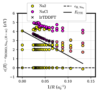
Figure 5: Eigenvalues of the Na₂–NaCl-system utilizing IVOs with $\hat{\Omega}_{k}^{S}$, where $k$ is the HOMO of the system located on Na₂. The Eigenvalues are given relative to the HOMO for $R\to\infty$ (dashed line) and their dependence on the inverse distance between the two molecules $\nicefrac{{1}}{{R}}$ is shown. The states are colored by their weight on the individual molecules. Solid line: eigenvalue of the LUMO of the NaCl molecule according to Mullikens law. The stars mark the CTE energies from TDDFT utilizing IVOs (fig. 4).

The possibility to calculate CTE by the combination of RSF and IVO by means of ground-state calculations is confirmed by fig. 5. It shows the eigenvalues of the HOMO as well as the eigenvalues of the unoccupied states of the Na₂–NaCl–System calculated by the utilization of the IVOs with $\hat{\Omega}_{k}^{\text{S}}$ as rotation operator in dependence of the intermolecular distance $R$ similar to figs. 1 and 4. In the asymptote $R\to\infty$ ($\frac{1}{R}\to 0$) the eigenvalues from the eigenstates of the isolated Na₂ molecule, which were subject to the modified Fock operator $\hat{F}^{\text{IVO}}$ with $\hat{\Omega}_{k}^{\text{S}}$, are shown. The eigenstates were colored by their weight on the individual molecules, where the projected local density of states was used. Similar to figs. 1 and 4 only states with an oscillator strength $\geq 10^{-2}$ for excitations from the Na₂-HOMO or $90\,\mathrm{\%}$ weight on NaCl are considered. For $R>\approx 10\,\mathrm{\text{\AA}}$ ($\frac{1}{R}\leq 0.05\,\mathrm{a_{0}^{-1}}$) the eigenvalue of the LUMO located on the NaCl molecule, which corresponds to the CTE state, is clearly visible and follows the straight line defined by Mullikens law with a constant slight offset. In this region the calculated eigenvalues of the LUMO are in perfect agreement with the energies predicted by lrTDDFT utilizing IVOs. The offset to Mullikens law is based on the difference between the eigenvalue of the NaCl LUMO and its calculated EA, see above. As in fig. 4 a second CTE state approximately one $\mathrm{eV}$ above the first CTE state can be identified.

While RSF open a way to calculate the energetics and oscillator strengths of Rydberg- and charge transfer excitations by lrTDDFT, the combination of RSF with IVOs opens a way to calculate the energetics of these excitations by means of ground-state calculations. Generalized lrTDDFT calculations using empty orbitals of the canonical FO need a much larger number of unoccupied states and thus are very hard to converge. This problem can be circumvented by utilizing IVOs that provide usable energies based on a rather small basis. But for lrTDDFT one needs to calculate Coulomb and exchange for every pair of excitation and de-excitation. Therefore lrTDDFT need a lot of computational resources compared to ground-state calculations. Thus utilizing the combination of RSF and IVOs one can calculate the energetics of CTEs on a light computational footprint.

VII Conclusions

In this article the implementation of RSFs utilizing the Slater function using the method of PAW on real space grids was presented. The screened Poisson equation was used to calculate the RSF exchange integrals on Cartesian grids, while integrations on radial grids were performed using the integration kernel devised by Rico et al..

The implementation was verified against literature, where excellent agreement has been found. Slight differences had been traced to the use of non-converged basis sets used in the literature, which underlines the importance of the basis set choice. Comparison between calculated and experimental mean ligand removal energies unveiled a poor description of binding situations including $d$-electrons by RSF and hybrid functionals that might be attributed of the poor treatment of $d$-binding in HFT.

lrTDDFT within the generalized Kohn-Sham scheme using canonical unoccupied Fock-orbitals is hard to converge as the empty states approximate (excited) electron affinities. These orbitals are thus inappropriate to describe neutral excitations. As a remedy, we combined Huzinaga’s IVOs with RSF and extended the linear response TDDFT coupling matrix accordingly. The RSF IVO orbitals are a superior basis for the calculation of excitations with much better convergence properties than these of the canonical FO. These orbitals and their energies not only improve the calculation of lrTDDFT. Due to their construction, they also open a way to calculate the energetics of CTEs by means of ground-state calculations. The much smaller numerical footprint of a ground state calculation as compared to lrTDDFT might enable calculation of these energies for systems unreachable by lrTDDFT.

Supporting information available

The evaluation of the local terms for the screened exchange, the influence of the grid-spacing and the amount of vacuum around each atom on the eigenvalues and derived energies, as well as the analytic expressions for the first, second and third derivative of the exchange term for an RSF with the use of the Slater function, the analytic solution of the screened Poisson equation for a Gaussian shaped density along with it’s derivation, the effects of dropping the projection operator $\hat{P}$ on the IVOs, excitation energies for the disodium molecule calculated by lrTDDFT utilizing RSF and IVOs with the three different forms of $\Omega_{k}$ and the rationale for the exchange terms in lrTDDFT are given in the supporting information.

Supporting information for “Calculation of charge transfer excitations with range separated functionals using improved virtual orbitals on real-space grids”

Introduction

This supporting information contains details of derivations and results that are too lengthy to be included in the main paper.

SI 1 Evaluation of local terms for screened exchange

As written in the main text, the evaluation of

$$\left(\left(n_{ij}\right)\right)^{\gamma} =\left(\left(\tilde{n}_{ij}\right)\right)^{\gamma}+\sum_{\alpha}\left[\left(\left(n^{\alpha}_{ij}\right)\right)^{\gamma}-\left(\left(\tilde{n}^{\alpha}_{ij}\right)\right)^{\gamma}\right],$$ (S1)

with

$$\left(\left(n_{ij}\right)\right)^{\gamma}=\left(n_{ij}|n_{ji}\right)^{\gamma}=\left(n_{ij}|\frac{\exp\left(-\gamma r_{12}\right)}{r_{12}}|n_{ji}\right)$$

would lead to cross-terms between localized functions located on different atomic sites and the need to integrate on incompatible gridsBlöchl (1994); Mortensen et al. (2005). To circumvent this, compensation charges $\tilde{Z}_{ij}^{\alpha}=\sum_{L}Q_{L,ij}^{\alpha}\hat{g}_{L}^{\alpha}$ with the expansion coefficients $Q_{L,ij}^{\alpha}$ and the smooth localized function $\hat{g}_{L}^{\alpha}$ are introducedRostgaard (2006); Enkovaara et al. (2010), where $L=(\ell,m)$ denotes the combination of angular $\ell$ and magnetic quantum numbers $m$.

Using $\tilde{\varrho}_{ij}=\tilde{n}_{ij}+\sum_{\alpha}\tilde{Z}_{ij}^{\alpha}$, eq. (S1) becomes

$$\left(\left(n_{ij}\right)\right)^{\gamma} =\left(\left(\tilde{\varrho}_{ij}\right)\right)^{\gamma}$$

$$\quad+\sum_{\alpha}\left[\left(\left(n^{\alpha}_{ij}\right)\right)^{\gamma}-\left(\left(\tilde{n}^{\alpha}_{ij}+\tilde{Z}_{ij}^{\alpha}\right)\right)^{\gamma}\right]$$ (S2)

$$=\left(\left(\tilde{\varrho}_{ij}\right)\right)^{\gamma}+\sum_{\alpha}\Delta K_{ij}^{\alpha\gamma}.$$ (S3)

The local correction term $\Delta K_{ij}^{\alpha\gamma}$ reads

$$\Delta K_{ij}^{\alpha\gamma} =\sum_{k_{1}k_{2}k_{3}k_{4}}\mathcal{P}_{ik_{1}}^{\alpha\ast}\mathcal{P}_{jk_{2}}^{\alpha}C_{k_{1}k_{2}k_{3}k_{4}}^{\alpha\gamma}\mathcal{P}_{jk_{3}}^{\alpha\ast}\mathcal{P}_{ik_{4}}^{\alpha}$$ (S4)

where the system independent tensor

$$C_{k_{1}k_{2}k_{3}k_{4}}^{\alpha\gamma} =J_{k_{1}k_{2}k_{3}k_{4}}^{\alpha\gamma}+$$

$$\quad\sum_{L}M_{k_{1}k_{2}}^{\alpha L\gamma}\Delta_{Lk_{3}k_{4}}^{\alpha}+$$

$$\quad\sum_{LL^{\prime}}\Delta_{Lk_{1}k_{2}}^{\alpha}N_{LL^{\prime}}^{\alpha\gamma}\Delta_{L^{\prime}k_{3}k_{4}}^{\alpha},$$ (S5)

with the terms

$$J_{k_{1}k_{2}k_{3}k_{4}}^{\alpha\gamma} =\frac{1}{2}\Big{[}\left(\phi_{k_{1}}^{\alpha}\phi_{k_{2}}^{\alpha}|\phi_{k_{3}}^{\alpha}\phi_{k_{4}}^{\alpha}\right)^{\gamma}$$

$$\left.\quad\quad\quad-\left(\tilde{\phi}_{k_{1}}^{\alpha}\tilde{\phi}_{k_{2}}^{\alpha}|\tilde{\phi}_{k_{3}}^{\alpha}\tilde{\phi}_{k_{4}}^{\alpha}\right)^{\gamma}\right]$$ (S6)

$$M_{k_{1}k_{2}}^{\alpha L\gamma} =\left(\tilde{\phi}_{k_{1}}^{\alpha}\tilde{\phi}_{k_{2}}^{\alpha}\big{|}\tilde{g}_{L}^{\alpha}\right)^{\gamma}$$ (S7)

$$N_{LL^{\prime}}^{\alpha\gamma} =\frac{1}{2}\left(\tilde{g}_{L}^{\alpha}|\tilde{g}_{L^{\prime}}^{\alpha}\right)^{\gamma},$$ (S8)

is used. The $\Delta_{Lk_{1}k_{2}}^{\alpha}$ are described in refs. 41; 58. Integrations on two types of grids have to be performed to evaluate $K^{\gamma}_{ij}$ by eq. (S3): once the integration on a three dimensional Cartesian grid using the soft pseudo-charge, $\tilde{\varrho}_{ij}$ and once integrations on a radial grid using the partial WF, $\phi_{k}^{\alpha}$, $\tilde{\phi}_{k}^{\alpha}$ and the localized function $\tilde{g}_{L}^{\alpha}$. The integration using the screened Poisson equation is discussed in the main text.

The partial wave functions $\phi_{k}^{\alpha}$ and the localized functions $\tilde{g}_{L}^{\alpha}$ are implemented as a (real) radial function $R_{k}(r)$ times a spherical harmonicsMortensen et al. (2005)

$$\phi^{\alpha}_{k} =R_{k}^{\alpha}(r)Y_{L_{k}}(\hat{r}).$$

Following the work of Rico et al.Rico et al. (2012), the screened exchange integral is evaluated on radial grids as

$$I_{k_{1}k_{2}k_{3}k_{4}}(\gamma)= 4\pi\sum_{L}G_{L_{k_{1}}L_{k_{2}}}^{L}G_{L_{k_{3}}L_{k_{4}}}^{L}$$

$$\quad\times\int_{0}^{\infty}R_{k_{1}}(r_{1})R_{k_{2}}(r_{1})r_{1}^{2}$$

$$\quad\times\int_{0}^{\infty}\frac{I_{\ell+\nicefrac{{1}}{{2}}}\left(\gamma r_{<}\right)K_{\ell+\nicefrac{{1}}{{2}}}\left(\gamma r_{>}\right)}{\sqrt{r_{1}r_{2}}}$$

$$\quad\times R_{k_{3}}(r_{2})R_{k_{4}}(r_{2})r_{2}^{2}dr_{1}dr_{2},$$ (S9)

where $G_{L_{a}L_{b}}^{L}$ denotes the Gaunt coefficientsGaunt (1929), $I_{\ell}(x)$ and $K_{\ell}(x)$ are the modified Bessel functions of the first and second type (the latter are also known as MacDonald functions)DLMF ; Olver et al. (2010), and $r_{>}$ and $r_{<}$ denote the smaller/larger of the radial coordinates $r_{1}$ and $r_{2}$. Note, that we have dropped the atomic index $\alpha$ for brevity.

SI 2 Influence of the grid- and vacuum-spacing on eigenvalues and energies

The grid-spacing $h$ and the amount of vacuum around each atom $x_{\text{vac}}$ are crucial parameters in grid-based calculations. To give a rationale for our chosen parameters, the influence of $h$ on the eigenvalues of the HOMO and the ionization energy for atomic chromium and oxygen is investigated.

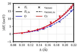
Figure SI 1: Deviation of $\epsilon_{\text{HOMO}}$ and $E_{\text{I}}$ for isolated a) oxygen and b) chromium atoms in dependence of the grid-spacing $h$.

Figure SI 1 depicts the absolute deviation $|\text{d}E|$ of the ionization energy $E_{\text{I}}$ and the eigenvalue of the HOMO $\epsilon_{\text{HOMO}}$ for atomic chromium and oxygen from the estimated value for an infinite dense grid relative to the grid-spacing. The value for the infinitely dense grid was estimated using an $h^{4}$ behavior. This was verified using a fit with $a\cdot h^{4}+b$ also depicted in fig. SI 1. The $h^{4}$ behavior is to be expected as all approximations in GPAW are exact to at least $h^{3}$Mortensen et al. (2005). LCY-PBE with $\gamma=0.9\,\mathrm{a_{0}^{-1}}$ was used in these calculations. This high value of the screening parameter leads to a strong decay of the screened Gaussian used to neutralize the charge introduced by calculating the exchange of a WF with itself. Both curves show a nearly identical behavior. For $h\leq 0.18\,\mathrm{\text{\AA}}$ both $E_{\text{I}}$ and $\epsilon_{\text{HOMO}}$ are converged within $10\,\mathrm{meV}$ relative to the estimated value for the infinite dense grid. Therefore $h=0.18\,\mathrm{\text{\AA}}$ was chosen for calculations not involving transition metals (which suffer from further numerical effects, see next section).

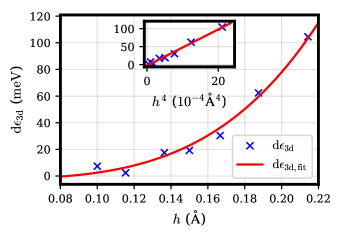
Figure SI 2: Energetic splitting, $\text{d}\epsilon_{3d}$, for the eigenvalues of the $3d$ shells of the isolated Chromium atom relative to the grid-spacing $h$.

The projection of $d$ type orbitals in transition metals on Cartesian grids leads to an artificial energetic splitting of the eigenvalues of the corresponding states. The influence of $h$ on this splitting was investigated in order to get parameters accurate for calculations involving transition metals. Figure SI 2 depicts the projection induced energetic splitting of the $3d$ shells $\text{d}\epsilon_{3d}$ for the example of atomic chromium. As indicated by the inset, the splitting also exhibits an $h^{4}$ behavior. The error for $h=0.18\,\mathrm{\text{\AA}}$ stays in the order of $50\,\mathrm{meV}$ and drops to $30\,\mathrm{meV}$ for $h=0.16\,\mathrm{\text{\AA}}$. Thus the latter spacing was chosen when transition metals were considered.

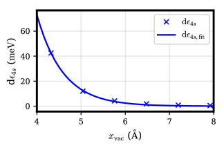
Figure SI 3: Eigenvalue of the occupied $4s$ orbital $\text{d}\epsilon_{4s}$ for an isolated Chromium atom relative to the distance of the atom from the border of the simulation box $x_{\text{vac}}$.

In order to study the effect of our finite simulation box, we have used the occupied $4s$ orbital of atomic chromium which is strongly delocalized. The behavior of its eigenvalue relative to $x_{\text{vac}}$ was taken as a measure to qualify an appropriate box-size. Figure SI 3 depicts the deviation of the eigenvalue of the occupied $4s$ orbital of the isolated Chromium atom from the estimated value for the infinite large simulation box relative to $x_{\text{vac}}$ for the functional LCY-PBE with $\gamma=0.9\,\mathrm{a_{0}}$. The deviation is below $30\,\mathrm{meV}$ already for $x_{\text{vac}}>4.5\,\mathrm{\text{\AA}}$. For $x_{\text{vac}}=6.0\,\mathrm{\text{\AA}}$ the differences falls below $5\,\mathrm{meV}$ which we regarded as adequate for the calculations performed.

SI 3 Derivatives of the localized range separation function

The exchange part of a GGA in the case of a Slater-function based RSF readsAkinaga and Ten-no (2008)

$$E_{\text{X}}^{\text{Slater}} =-\frac{1}{2}\sum_{\sigma}\int\text{d}\vec{r}K_{\sigma}^{\text{GGA}}\varrho_{\sigma}^{\frac{4}{3}}$$

$$\quad\times\underbrace{\left[1-\frac{8}{3}a_{\sigma}\left\{\arctan\frac{1}{a_{\sigma}}+\frac{a_{\sigma}}{4}-\frac{a_{\sigma}}{4}\left(a_{\sigma}^{2}+3\right)\ln\left(1+\frac{1}{a_{\sigma}^{2}}\right)\right\}\right]}_{=f(a_{\sigma})},$$ (S10)

where $\sigma$ denotes the spin, $K_{\sigma}^{\text{GGA}}$ the GGA correction, $a_{\sigma}$ = $\gamma/2k_{\sigma}^{\text{GGA}}$ with $k_{\sigma}^{\text{GGA}}=\left(9\pi/K_{\sigma}^{\text{GGA}}\right)^{\frac{1}{2}}\varrho_{\sigma}^{\frac{1}{3}}$ as given in refs. Akinaga and Ten-no (2008); Iikura et al. (2001). To calculate the exchange-correlation potential

$$v_{\text{XC}}[\varrho_{\sigma}](\vec{r})=\frac{\delta E_{\text{XC}}}{\delta\varrho_{\sigma}(\vec{r})},$$ (S11)

the exchange-correlation kernel

$$f_{\text{XC}}[\varrho_{\sigma},\varrho_{\sigma}^{\prime}](\vec{r},\vec{r\prime})=\frac{\delta^{2}E_{\text{XC}}}{\delta\varrho_{\sigma}(\vec{r})\delta\varrho_{\sigma}^{\prime}(\vec{r}^{\prime})},$$ (S12)

and the exchange-correlation hyper-kernel

$$k_{\text{XC}}[\varrho_{\sigma},\varrho_{\sigma}^{\prime},\varrho_{\sigma}^{\prime\prime}](\vec{r},\vec{r\prime},\vec{r\prime\prime})=\frac{\delta^{3}E_{\text{XC}}}{\delta\varrho_{\sigma}(\vec{r})\delta\varrho_{\sigma}^{\prime}(\vec{r}^{\prime})\delta\varrho_{\sigma}^{\prime\prime}(\vec{r}^{\prime\prime})},$$ (S13)

the first, second and third derivative of the second line of eq. (S10) regarding to the density or using the chain rule and the definitions given by refs. Akinaga and Ten-no (2008); Iikura et al. (2001) to $a_{\sigma}$ are needed. These are

$$\frac{\partial f(a_{\sigma})}{\partial a_{\sigma}} =\frac{4}{3}\left(\left(2a_{\sigma}^{3}+3a_{\sigma}\right)\ln\left(1+\frac{1}{a_{\sigma}^{2}}\right)\right.$$

$$\quad\quad\quad\left.-2a_{\sigma}-2\arctan\left(\frac{1}{a_{\sigma}}\right)\right),$$ (S14)

$$\frac{\partial^{2}f(a_{\sigma})}{\partial a_{\sigma}^{2}} =4\left(\left((2a_{\sigma}^{2}+1\right)\ln\left(1+\frac{1}{a_{\sigma}^{2}}\right)-2\right),$$ (S15)

$$\frac{\partial^{3}f(a_{\sigma})}{\partial a_{\sigma}^{3}} =\frac{8\left(\left(2a_{\sigma}^{4}+2a_{\sigma}^{2}\right)\ln\left(1+\frac{1}{a_{\sigma}^{2}}\right)-2a_{\sigma}^{2}-1\right)}{a_{\sigma}^{3}+a_{\sigma}}.$$ (S16)

SI 4 Solution of the integral for a Gaussian shaped density times the Yukawa potential

A Gaussian distributed charge is subtracted in case of charged systems in order to work with the (modified) Poisson equation for involving a neutral charge density. This strategy involves the integral of a parametrized Gaussian shaped density $n(\vec{r},\vec{r_{0}},\sigma)$ times the Yukawa potential $f(\vec{r},\vec{r^{\prime}},\gamma)$, which reads

$$I =\int n(\vec{r},\vec{r_{0}},\sigma)f(\vec{r},\vec{r}^{\prime},\gamma)\text{d}^{3}\vec{r}$$ (S17)

$$=\int\underbrace{\exp\left(-\frac{\left(\vec{r}-\vec{r_{0}}\right)^{2}}{2\sigma^{2}}\right)}_{=n(\vec{r},\vec{r_{0}},\sigma)}\underbrace{\frac{e^{-\gamma|\vec{r}^{\prime}-\vec{r}|}}{|\vec{r}^{\prime}-\vec{r}|}}_{=f(\vec{r},\vec{r}^{\prime},\gamma)}\text{d}^{3}\vec{r}\;.$$ (S18)

This can be rewritten as

$$I =\int\exp\left(-\frac{\left(\vec{\varrho_{0}}-\vec{\varrho}^{\prime}\right)^{2}}{2\sigma^{2}}\right)\frac{e^{-\gamma|\vec{\varrho}^{\prime}|}}{|\vec{\varrho}^{\prime}|}\text{d}^{3}\varrho^{\prime}$$ (S19)

by substituting $\vec{\varrho}^{\prime}=\vec{r}^{\prime}-\vec{r}$ and $\vec{\varrho_{0}}=\vec{r}^{\prime}-\vec{r_{0}}$. Using spherical coordinates and completing the square in the exponent, the integral can be written as

$$I =\int_{0}^{2\pi}\text{d}\varphi\int_{0}^{\pi}\sin\theta\text{d}\theta$$

$$\quad\times\int_{0}^{R}\varrho^{2}\frac{e^{-\gamma\left|\vec{\varrho}\right|}}{\left|\vec{\varrho}\right|}\exp\left(-\frac{\varrho^{2}+\varrho_{0}^{2}-2\varrho\varrho_{0}\cos\theta}{2\sigma^{2}}\right)\text{d}\varrho\;.$$ (S20)

After solving the angular integrals, the remaining integral reads (for infinite $R$)

$$I =2\pi\frac{\sigma^{2}}{\varrho_{0}}e^{-\frac{\varrho_{0}^{2}}{2\sigma^{2}}}$$

$$\quad\times\int_{0}^{\infty}\left(e^{\frac{\varrho_{0}\varrho}{\sigma^{2}}}-e^{-\frac{\varrho_{0}\varrho}{\sigma^{2}}}\right)e^{-\gamma\varrho}e^{-\frac{\varrho^{2}}{2\sigma^{2}}}\text{d}\varrho\;,$$ (S21)

which can be divided into two parts

$$I_{1} =2\pi\frac{\sigma^{2}}{\varrho_{0}}e^{-\frac{\varrho_{0}^{2}}{2\sigma^{2}}}\int_{0}^{\infty}e^{\frac{\varrho_{0}\varrho}{\sigma^{2}}}e^{-\gamma\varrho}e^{-\frac{\varrho^{2}}{2\sigma^{2}}}\text{d}\varrho$$ (S22)

$$=2\pi\frac{\sigma^{2}}{\varrho_{0}}e^{-\frac{\varrho_{0}^{2}}{2\sigma^{2}}}$$

$$\quad\times\exp\left(\frac{\left(\sigma^{2}\gamma-\varrho_{0}\right)^{2}}{2\sigma^{2}}\right)\sigma\sqrt{\frac{\pi}{2}}\operatorname{erfc}\left(\frac{\sigma^{2}\gamma-\varrho_{0}}{\sqrt{2}\sigma}\right),$$ (S23)

and

$$I_{2} =-2\pi\frac{\sigma^{2}}{\varrho_{0}}e^{-\frac{\varrho_{0}^{2}}{2\sigma^{2}}}\int_{0}^{\infty}e^{-\frac{\varrho_{0}\varrho}{\sigma^{2}}}e^{-\gamma\varrho}e^{-\frac{\varrho^{2}}{2\sigma^{2}}}\text{d}\varrho$$ (S24)

$$=-2\pi\frac{\sigma^{2}}{\varrho_{0}}e^{-\frac{\varrho_{0}^{2}}{2\sigma^{2}}}$$

$$\quad\times\exp\left(\frac{\left(\sigma^{2}\gamma+\varrho_{0}\right)^{2}}{2\sigma^{2}}\right)\sigma\sqrt{\frac{\pi}{2}}\operatorname{erfc}\left(\frac{\sigma^{2}\gamma+\varrho_{0}}{\sqrt{2}\sigma}\right).$$ (S25)

Combining these results leads to

$$I_{1}+I_{2} =\frac{\sigma^{3}\pi^{3/2}\sqrt{2}}{\varrho_{0}}e^{\frac{\sigma^{2}\gamma^{2}}{2}}$$

$$\quad\times\left[\exp\left(-\gamma\varrho_{0}\right)\operatorname{erfc}\left(\frac{\sigma^{2}\gamma-\varrho_{0}}{\sqrt{2}\sigma}\right)\right.$$

$$\left.\quad\quad-\exp\left(\gamma\varrho_{0}\right)\operatorname{erfc}\left(\frac{\sigma^{2}\gamma+\varrho_{0}}{\sqrt{2}\sigma}\right)\right]\;.$$ (S26)

By comparison of the density $n(\vec{r},\vec{r_{0}},\sigma)$ from eq. (S18) with a normalized Gaussian

$$n(\vec{r},\vec{r_{0}},\sigma) =\frac{1}{\left(2\pi\right)^{3/2}\sigma^{3}}\exp\left(-\frac{\left(\vec{r}-\vec{r_{0}}\right)^{2}}{2\sigma^{2}}\right),$$ (S27)

the potential for a screened normalized Gaussian can be written as

$$\varphi(\varrho_{0},\gamma,\sigma) =\frac{1}{2\varrho_{0}}e^{\frac{\sigma^{2}\gamma^{2}}{2}}$$

$$\quad\times\left[\exp\left(-\gamma\varrho_{0}\right)\operatorname{erfc}\left(\frac{\sigma^{2}\gamma-\varrho_{0}}{\sqrt{2}\sigma}\right)\right.$$

$$\left.\quad\quad-\exp\left(\gamma\varrho_{0}\right)\operatorname{erfc}\left(\frac{\sigma^{2}\gamma+\varrho_{0}}{\sqrt{2}\sigma}\right)\right].$$ (S28)

According to the computer algebra system maximaMaxima (2014) this converges to the error-function divided by $\varrho_{0}$ for $\gamma\to 0$

$$\lim_{\gamma\to 0}\varphi(\varrho_{0},\gamma,\sigma) =-\frac{\operatorname{erfc}\left(\frac{\varrho_{0}}{\sqrt{2}\sigma}\right)-1}{\varrho_{0}}$$ (S29)

$$=\frac{\operatorname{erf}\left(\frac{\varrho_{0}}{\sqrt{2}\sigma}\right)}{\varrho_{0}},$$ (S30)

which is known as the Coulomb potential of a Gaussian shaped charge densityJackson (1998).

SI 5 Comparsion of the eigenvalues for Be₂

$n$	$f_{n}$	$\epsilon_{\hat{F}^{\text{IVO}}_{\text{Huz}}}\,\mathrm{(eV)}$	$\epsilon_{\hat{F}^{\text{IVO}}_{\text{Kel}}}\,\mathrm{(eV)}$	$\epsilon_{\hat{F}^{\text{IVO}}_{\text{Kel}}(n_{\text{max}}=15)}\,\mathrm{(eV)}$
0	2	$-10.47$	$-10.47$	$-10.47$
1	2	$-7.49$	$-7.49$	$-7.49$
2	0	$-5.23$	$-5.23$	$-5.23$
3	0	$-5.23$	$-5.23$	$-5.23$
4	0	$-3.51$	$-3.48$	$-3.49$
5	0	$-2.33$	$-2.34$	$-2.34$
6	0	$-2.33$	$-2.34$	$-2.34$
7	0	$-1.95$	$-1.94$	$-1.95$

Table SI 1: Comparison of the eigenvalues of the Be₂ molecule using the different modified Fock operators. $n$ band-index, $f_{\text{n}}$ occupation number. Gridspacing $h=0.25\,\mathrm{\text{\AA}}$, amount of vacuum around the atoms, $x_{\text{vac}}=6\,\mathrm{\text{\AA}}$.

To verify the effects of dropping $\hat{P}$ in eq. (20) of the main text, a HFT calculation using the modified Fock operator from Huzinaga, $\epsilon_{\hat{F}^{\text{IVO}}_{\text{Huz}}}$, including the projection operator $\hat{P}$ is compared to two calculations which use the rotation operator $\Omega_{k}$, but drop the usage of $\hat{P}$ and blank the HFT exchange cross-elements between occupied and unoccupied states $\epsilon_{\hat{F}^{\text{IVO}}_{\text{Kel}}}$. The results are listed in tab. SI 1. The calculated eigenvalues are nearly identical, such that the procedure of dropping $\hat{P}$ and blanking the cross term is suitable for the calculation of excited states using eigenvalue-differences or lrTDDFT.

SI 6 Including RSF in lrTDDFT

We consider the changes brought into generalized lrTDDFT through the terms from range separated functionals. The most general case is the CAM scheme, where the Coulomb interaction kernel of the exchange integral, eq. (3) in the main text, is split into two parts Yanai et al. (2004)

$$\frac{1}{r_{12}}= \underbrace{\frac{1-\left[\alpha+\beta\left(1-\omega_{\text{RSF}}(\gamma,r_{12})\right)\right]}{r_{12}}}_{\text{SR, DFT}}+\underbrace{\frac{\alpha+\beta\left(1-\omega_{\text{RSF}}(\gamma,r_{12})\right)}{r_{12}}.}_{\text{LR, HFT}}$$ (S31)

In linear response TDDFT or TDHFT we have to solve the generalized eigenvalue problemDreuw et al. (2003); Casida (2009); Akinaga and Ten-No (2009)

$$\begin{pmatrix}\mathbf{A}&\mathbf{B}\\ \mathbf{B^{\ast}}&\mathbf{A^{\ast}}\end{pmatrix}\begin{pmatrix}\vec{X}\\ \vec{Y}\end{pmatrix} =\omega\begin{pmatrix}\mathbf{1}&\mathbf{0}\\ \mathbf{0}&-\mathbf{1}\end{pmatrix}\begin{pmatrix}\vec{X}\\ \vec{Y}\end{pmatrix},$$ (S32)

with

$$A_{ia\sigma,jb\tau} =\delta_{ij}\delta_{ab}\delta_{\sigma\tau}\left(\epsilon_{a}-\epsilon_{i}\right)+K_{ia\sigma,jb\tau}$$ (S33)

$$B_{ia\sigma,jb\tau} =K_{ia\sigma,bj\tau}$$ (S34)

and the element $K_{pq\sigma,rs\tau}$ of the lrTDDFT coupling matrix readsCasida (2009)

$$K_{pq\sigma,rs\tau}^{\text{HFT}} =\left(pq|rs\right)-\delta_{\sigma\tau}\left(pr|sq\right)$$ for HFT (S35)

$$K_{pq\sigma,rs\tau}^{\text{DFT}} =\left(pq|rs\right)+\left(pq|f_{\text{XC}}|rs\right) \text{for DFT},$$ (S36)

where $p,q,r,s$ denotes arbitrary orbital-indices, $\sigma$ and $\tau$ are spin-indices, which are left out for brevity if selected by the Kronecker delta, $\delta_{\sigma\tau}$. $f_{\text{xc}}=\frac{\delta^{2}E_{\text{xc}}}{\delta\varrho\left(\vec{r_{1}}\right)\delta\varrho\left(\vec{r_{2}}\right)}$ denotes the exchange-correlation kernel of the functional. Mulliken like notations

$$\left(pq|rs\right) =\int\int\frac{p^{\ast}(\vec{r_{1}})q(\vec{r_{1}})r^{\ast}(\vec{r_{2}})s(\vec{r_{2}})}{|\vec{r_{1}}-\vec{r_{2}}|}\text{d}\vec{r_{1}}\text{d}\vec{r_{2}}$$ (S37)

and

$$\left(pq|\hat{x}|rs\right) =\int\int p^{\ast}(\vec{r_{1}})q(\vec{r_{1}})\hat{x}(\vec{r_{1}},\vec{r_{2}},...)r^{\ast}(\vec{r_{2}})s(\vec{r_{2}})\text{d}\vec{r_{1}}\text{d}\vec{r_{2}}$$ (S38)

are used. The first terms in eqs. (S35) and (S36) are the so called RPA terms, exchange and correlation plugs into the second terms.

Applying eq. (S31) into the exchange-dependent terms, and keeping in mind that the HFT-exchange is negative $E_{\text{X}}^{\text{HFT}}=-\frac{1}{2}\sum_{ij}(ij|ji)$, we get

$$K_{pq\sigma,rs\tau} =\left(p_{\sigma}q_{\sigma}|r_{\tau}s_{\tau}\right)+K_{pq\sigma,rs\tau}^{\text{CAM-DFT}}+K_{pq\sigma,rs\tau}^{\text{CAM-HFT}}$$ (S39)

with

$$K_{pq\sigma,rs\tau}^{\text{CAM-DFT}} =\left(1-\alpha-\beta\right)\left(p_{\sigma}q_{\sigma}|f_{\text{xc}}|r_{\tau}s_{\tau}\right)+\beta\left(p_{\sigma}q_{\sigma}|f_{\text{xc}}^{\text{RSF}}|r_{\tau}s_{\tau}\right)$$ (S40)

$$K_{pq\sigma,rs\tau}^{\text{CAM-HFT}} =-\delta_{\sigma\tau}\left(pr|\frac{\alpha+\left(1-\omega_{\text{RSF}}\right)}{r_{12}}|sq\right),$$ (S41)

where $f_{\text{XC}}^{RSF}$ denotes the dampened kernel of the RSF.

This resembles a global hybrid for $\alpha\neq 0$ and $\beta=0$Dreuw et al. (2003)

$$K_{pq\sigma,rs\tau} =\left(pq\sigma|rs\tau\right)+\left(1-\alpha\right)K^{\text{DFT}}_{pq\sigma,rs\tau}+\alpha K^{\text{HFT}}_{pq\sigma,rs\tau}$$ (S42)

with

$$K^{\text{DFT}}_{pq\sigma,rs\tau} =\left(pq\sigma|f_{\text{XC}}|rs\tau\right)$$ (S43)

$$K^{\text{HFT}}_{pq\sigma,rs\tau} =-\delta_{\sigma\tau}\left(pr|sq\right)$$ (S44)

and the pure LC scheme for $\alpha=0$, $\beta=1$ Kuritz et al. (2011)

$$K_{pq\sigma,rs\tau} =\left(pq\sigma|rs\tau\right)+\beta K^{\text{LC-DFT}}_{pq\sigma,rs\tau}+\beta K^{\text{HFT}}_{pq\sigma,rs\tau}$$ (S45)

with

$$K^{\text{DFT}}_{pq\sigma,rs\tau} =\left(pq\sigma|f_{\text{XC}}^{\text{RSF}}|rs\tau\right)$$ (S46)

$$K^{\text{HFT}}_{pq\sigma,rs\tau} =-\delta_{\sigma\tau}\left(pr|\frac{1-\omega_{\text{RSF}}}{r_{12}}|sq\right)\,.$$ (S47)

Note, that the sign of the last (HFT) term in eqs. (S39) and (S41) is erroneously positive in refs. Tawada et al. (2004) and Akinaga and Ten-No (2009).

SI 7 Impact of different forms of the IVO operator on excitions in Na₂

state	Exp.	$\Omega_{k}^{S}$				$\Omega_{k}^{A}$				$\Omega_{k}^{T}$
	(eV)	$e_{\nu}\mathrm{(eV)}$		$f_{\nu}$		$e_{\nu}\mathrm{(eV)}$		$f_{\nu}$		$e_{\nu}\mathrm{(eV)}$		$f_{\nu}$
a ${}^{3}\Sigma_{u}^{+}$	$0.71$	$0.66$	$(0.68)$	$0.$	$(0.)$	$0.62$	$(0.64)$	$0.$	$(0.)$	$0.57$	$(0.58)$	$0.$	$(0.)$
b ${}^{3}\Pi_{u}$	$1.68$	$1.41$	$(1.56)$	$0.$	$(0.)$	$1.38$	$(1.45)$	$0.$	$(0.)$	$1.36$	$(1.37)$	$0.$	$(0.)$
A ${}^{1}\Sigma_{u}^{+}$	$1.81$	$2.09$	$(2.10)$	$0.83$	$(0.84)$	$2.09$	$(2.10)$	$0.64$	$(0.65)$	$2.08$	$(2.12)$	$0.44$	$(0.45)$
1 ${}^{3}\Sigma_{g}^{+}$	$2.25$	$2.37$	$(2.41)$	$0.$	$(0.)$	$2.36$	$(2.47)$	$0.$	$(0.)$	$2.35$	$(2.39)$	$0.$	$(0.)$
B ${}^{1}\Pi_{u}$	$2.52$	$2.61$	$(2.68)$	$1.38$	$(1.50)$	$2.62$	$(2.75)$	$1.16$	$(1.32)$	$2.63$	$(2.85)$	$0.94$	$(1.06)$

Table SI 2: Excitation-energies and oscillator-strengths of Na₂ calculated by lrTDDFT utilizing the combination of RSF and IVOs. Experimental energies (Exp.) and state assignments from refs. Huber and Herzberg (2016); Li and Lyyra (1999). $e_{\nu}$: excitation energy, $f_{\nu}$: oscillator strength. $\Omega_{k}^{S,A,T}$: values calculated using the according rotation-operator. A large basis of 100 unoccupied states was used, while the values in brackets use a small basis of seven unoccupied states only. The gridspacing was set to $h=0.20\,\mathrm{\text{\AA}}$ and the simulation box contained at least $x_{\text{vac}}=11\,\mathrm{\text{\AA}}$ around each atom.

We now discuss the changes introduced by IVOs to the linear response matrices in HFTBerman and Kaldor (1979). The matrix $\mathcal{B}$ is the same as with canonical HFT unoccupied orbitals. The changes on the $\mathcal{A}$ matrix in HFT

$$\mathbf{A}^{\text{HFT}}_{ia\sigma,jb\tau} =\delta_{ij}\delta_{ab}\delta_{\sigma\tau}\left(\epsilon_{a\sigma}-\epsilon_{i\tau}\right)+K_{ia\sigma,jb\tau}$$ (S48)

$$=\delta_{ij}\delta_{ab}\delta_{\sigma\tau}\left(\epsilon_{a\sigma}-\epsilon_{i\tau}\right)+\left(i_{\sigma}a_{\sigma}|j_{\tau}b_{\tau}\right)-\delta_{\sigma\tau}\left(i_{\sigma}j_{\sigma}|a_{\tau}b_{\tau}\right)$$ (S49)

by applying the operator of eq. (27) in the main text are

$$\mathbf{A}^{\text{IVO}}_{ia\sigma,jb\tau} =\delta_{ij}\delta_{ab}\delta_{\sigma\tau}\left(\epsilon_{a\sigma}^{\text{IVO}}-\epsilon_{i\tau}\right)+\left(i_{\sigma}a_{\sigma}|j_{\tau}b_{\tau}\right)-\delta_{\sigma\tau}\left(i_{\sigma}j_{\sigma}|a_{\tau}b_{\tau}\right)$$

$$\quad+\delta_{ab}\delta_{\sigma\tau}\left[\left(a_{\sigma}a_{\sigma}|k_{\tau}k_{\tau}\right)-\left(a_{\sigma}k_{\sigma}|k_{\tau}a_{\tau}\right)\mp\left(a_{\sigma}k_{\sigma}|k_{\tau}a_{\tau}\right)\right]\;,$$ (S50)

where the negative sign is to be used for singlets, the positive sign for triplets. Disregarding changes in the wavefunctions, the IVOs change the eigenvalue $\epsilon_{a}^{\text{IVO}}$ as compared to the canonical unoccupied states value $\epsilon_{a}$ to

$$\epsilon_{a}^{\text{IVO}} =\epsilon_{a}-\left(aa|kk\right)+\left(ak|ka\right)\pm\left(ak|ka\right),$$ (S51)

where the positive (negative) sign is for singlets (triplets). Therefore $\mathbf{A}^{\text{IVO}}_{ia\sigma,jb\tau}$ becomes

$$\mathbf{A}^{\text{IVO}}_{ia\sigma,jb\tau} =\delta_{\sigma\tau}\{\delta_{ab}\left[\delta_{ij}\left(\epsilon_{a_{\sigma}}-\left(a_{\sigma}a_{\sigma}|k_{\tau}k_{\tau}\right)+\left(a_{\sigma}k_{\sigma}|k_{\tau}a_{\tau}\right)\pm\left(a_{\sigma}k_{\sigma}|k_{\tau}a_{\tau}\right)-\epsilon_{i\tau}\right)\right.$$

$$\quad\quad\quad\quad\left.+\left(a_{\sigma}a_{\sigma}|k_{\tau}k_{\tau}\right)-\left(a_{\sigma}k_{\sigma}|k_{\tau}a_{\tau}\right)\mp\left(a_{\sigma}k_{\sigma}|k_{\tau}a_{\tau}\right)\right]-\left(i_{\sigma}j_{\sigma}|a_{\tau}b_{\tau}\right)\}$$

$$\quad\quad+\left(i_{\sigma}a_{\sigma}|j_{\tau}b_{\tau}\right)$$ (S52)

If we discuss a single, isolated excitation (single pole approximation, SPA, $i=j$, $a=b$), eq. (S49) becomes:

$$\mathbf{A}_{ia\sigma,ia\tau}^{\text{HFT,SPA}} =\delta_{\sigma\tau}\left(\epsilon_{a\sigma}-\epsilon_{i\tau}\right)+\left(i_{\sigma}a_{\sigma}|i_{\tau}a_{\tau}\right)-\delta_{\sigma\tau}\left(i_{\sigma}i_{\sigma}|a_{\tau}a_{\tau}\right),$$ (S53)

and eq. (S52) becomes (using $a^{\prime}$ for the IVO orbitals):

$$\mathbf{A}_{ia^{\prime}\sigma,ia^{\prime}\tau}^{\text{IVO,SPA}} =\delta_{\sigma\tau}\{\epsilon_{a\sigma}-\left(a_{\sigma}^{\prime}a_{\sigma}^{\prime}|k_{\tau}k_{\tau}\right)+\left(a_{\sigma}^{\prime}k_{\sigma}|k_{\tau}a_{\tau}^{\prime}\right)\pm\left(a_{\sigma}^{\prime}k_{\sigma}|k_{\tau}a_{\tau}^{\prime}\right)-\epsilon_{i_{\tau}}$$

$$\quad\quad\quad\quad+\left(a_{\sigma}^{\prime}a_{\sigma}^{\prime}|k_{\tau}k_{\tau}\right)-\left(a_{\sigma}^{\prime}k_{\sigma}|k_{\tau}a_{\tau}^{\prime}\right)\mp\left(a_{\sigma}^{\prime}k_{\sigma}|k_{\tau}a_{\tau}^{\prime}\right)-\left(i_{\sigma}i_{\sigma}|a_{\tau}^{\prime}a_{\tau}^{\prime}\right)\}$$

$$\quad\quad+\left(i_{\sigma}a^{\prime}_{\sigma}|i_{\tau}a^{\prime}_{\tau}\right)$$ (S54)

$$=\delta_{\sigma\tau}\{\epsilon_{a\sigma}-\epsilon_{i\tau}-\left(i_{\sigma}i_{\sigma}|a_{\tau}^{\prime}a_{\tau}^{\prime}\right)\}+\left(i_{\sigma}a^{\prime}_{\sigma}|i_{\tau}a^{\prime}_{\tau}\right)$$ (S55)

Eqs. (S53) are (S55) equal for $a=a^{\prime}$, but $a$ and $a^{\prime}$ are eigenfunctions to different operators, thus eqs. (S53) and (S55) will lead to different results. Thus the excitation energies have to differ in SPA. This also holds true for the eigenfunction of the different operators $\Omega_{k}^{S,A,T}$ between each other. We’ve calculated the excitation energies and oscillator strengths for the isolated Na₂ molecule using the different operators for a small, seven, and a larger number of unoccupied states. The calculated values are listed in tab. SI 2. The energies generally agree within $100\,\mathrm{meV}$, while singlet energies agree even within $20\,\mathrm{meV}$.

Tab. SI 2 also reveals, that there are differences in the oscillator strengths obtained with the three operators. The oscillator strengths are calculated byWalter et al. (2008)

$$f_{I\alpha} =\frac{2m_{e}}{\hbar e^{2}}\left|\sum_{ia\sigma}\left(\vec{\mu}_{ia\sigma}\right)_{\alpha}\sqrt{\epsilon_{ia\sigma}}\left(F_{\text{I}}\right)_{ia\sigma}\right|^{2}$$ (S56)

where $\epsilon_{ia\sigma}=\epsilon_{a\sigma}-\epsilon_{i\sigma}$ denotes the eigenvalue-differences of the individual occupied $i$ and unoccupied $a$ Kohn-Sham (KS) states. The $\vec{\mu}_{ia\sigma}=-e\langle i\sigma|\vec{r}|a\sigma\rangle$ are the KS transition dipoles and $F_{I}$ denotes the eigenvector of the $\Omega$ matrix.

	$\Omega_{k}^{S}$	$\Omega_{k}^{A}$	$\Omega_{k}^{T}$
$f_{ia\sigma}$	$0.43$	$0.33$	$0.23$
$\epsilon_{ia\sigma}(\mathrm{eV})$	$1.99$	$1.54$	$1.06$
$\nicefrac{{f_{ia\sigma}}}{{\epsilon_{ia\sigma}}}(\nicefrac{\mathrm{1}}{\mathrm{eV}})$	$0.22$	$0.21$	$0.22$

Table SI 3: Oscillator strengths $f_{ia\sigma}$ of eq. (S57), for the HOMO-LUMO transition, where the LUMO is obtained using different forms of the IVO operator $\Omega_{k}^{S,A,T}$. The corresponding excitation energies $\epsilon_{ia\sigma}=\epsilon_{a\sigma}-\epsilon_{i\sigma}$ and the ratios are also given. Numerical settings as in tab. SI 2.

The differences in the oscillator strengths arise from differences in the single particle energy differences $\epsilon_{ia\sigma}$. In order to show this the mean KS oscillator strengths

$$f_{ia\sigma} =\frac{2m_{e}}{3\hbar e^{2}}\;\epsilon_{ia\sigma}\sum_{\alpha=x,y,z}\left|\left(\vec{\mu}_{ia\sigma}\right)_{\alpha}\right|^{2}$$ (S57)

are given in tab. SI 3 for a single KS transition from HOMO to LUMO, where $\alpha$ denotes the spatial direction of $\vec{\mu}$. The value of $\epsilon_{a\sigma}$ depends on $\Omega_{k}^{S,A,T}$ which is reflected in $\epsilon_{ia\sigma}$. While excitation energies and the oscillator strengths differ by up to a factor of two, their ratio is practically constant. The variance in KS transition energies is compensated in $\mathbf{A}^{\text{IVO}}$, but not in the matrix elements.

References

- Sariciftci et al. (1992) N. S. Sariciftci, L. Smilowitz, A. J. Heeger, and F. Wudl, Science 258, 1474 (1992).
- Samorí et al. (2002) P. Samorí, N. Severin, C. D. Simpson, K. Müllen, and J. P. Rabe, J. Am. Chem. Soc. 124, 9454 (2002).
- Blundell and Pratt (2004) S. J. Blundell and F. L. Pratt, J. Phys.: Condens. Matter 16, R771 (2004).
- Mulliken and Person (1969) R. S. Mulliken and W. B. Person, Molecular Complexes: A Lecture and Reprint Volume (Wiley-Interscience, New York; London, 1969) oCLC: 499972894.
- Hohenberg and Kohn (1964) P. Hohenberg and W. Kohn, Phys. Rev. 136, B864 (1964).
- Kohn and Sham (1965) W. Kohn and L. J. Sham, Phys. Rev. 140, A1133 (1965).
- Livshits and Baer (2007) E. Livshits and R. Baer, Phys. Chem. Chem. Phys. 9, 2932 (2007), arXiv:0701493 [cond-mat] .
- Chai and Head-Gordon (2008) J.-D. Chai and M. Head-Gordon, J. Chem. Phys. 128, 084106 (2008).
- Cohen et al. (2008) A. J. Cohen, P. Mori-Sánchez, and W. Yang, Science 321, 792 (2008).
- Baer et al. (2010) R. Baer, E. Livshits, and U. Salzner, Annu. Rev. Phys. Chem. 61, 85 (2010).
- Vosko et al. (1980) S. H. Vosko, L. Wilk, and M. Nusair, Can. J. Phys. 58, 1200 (1980).
- Perdew and Zunger (1981) J. P. Perdew and A. Zunger, Phys. Rev. B 23, 5048 (1981).
- Perdew and Wang (1992) J. P. Perdew and Y. Wang, Phys. Rev. B 45, 13244 (1992).
- Gill (1996) P. M. W. Gill, Mol. Phys. 89, 433 (1996).
- Perdew et al. (1996) J. P. Perdew, K. Burke, and M. Ernzerhof, Phys. Rev. Lett. 77, 3865 (1996).
- Adamo et al. (2000) C. Adamo, M. Ernzerhof, and G. E. Scuseria, J. Chem. Phys. 112, 2643 (2000).
- Tao et al. (2003) J. Tao, J. P. Perdew, V. N. Staroverov, and G. E. Scuseria, Phys. Rev. Lett. 91, 146401 (2003), arXiv:0306203 [cond-mat] .
- Becke (1993) A. D. Becke, J. Chem. Phys. 98, 1372 (1993).
- Baer and Neuhauser (2005) R. Baer and D. Neuhauser, Phys. Rev. Lett. 94, 043002 (2005), arXiv:0408664 [cond-mat] .
- Dreuw et al. (2003) A. Dreuw, J. L. Weisman, and M. Head-Gordon, J. Chem. Phys. 119, 2943 (2003).
- Baerends et al. (2013) E. J. Baerends, O. V. Gritsenko, and R. van Meer, Phys. Chem. Chem. Phys. 15, 16408 (2013).
- Kümmel (2017) S. Kümmel, Adv. Energy Mater. 7, 1700440 (2017).
- Maitra (2017) N. T. Maitra, Journal of Physics: Condensed Matter 29, 423001 (2017), arXiv:1707.08054 [physics.chem-ph] .
- Tawada et al. (2004) Y. Tawada, T. Tsuneda, S. Yanagisawa, T. Yanai, and K. Hirao, J. Chem. Phys. 120, 8425 (2004).
- Akinaga and Ten-No (2009) Y. Akinaga and S. Ten-No, Int. J. Quantum Chem. 109, 1905 (2009).
- Rohrdanz et al. (2009) M. A. Rohrdanz, K. M. Martins, and J. M. Herbert, J. Chem. Phys. 130, 054112 (2009).
- Stein et al. (2009a) T. Stein, L. Kronik, and R. Baer, J. Am. Chem. Soc. 131, 2818 (2009a).
- Stein et al. (2009b) T. Stein, L. Kronik, and R. Baer, J. Chem. Phys. 131, 244119 (2009b).
- Kronik et al. (2012) L. Kronik, T. Stein, S. Refaely-Abramson, and R. Baer, J. Chem. Theory Comput. 8, 1515 (2012).
- Zhang et al. (2012) X. Zhang, Z. Li, and G. Lu, J. Phys.: Condens. Matter 24, 205801 (2012).
- Yanai et al. (2004) T. Yanai, D. P. Tew, and N. C. Handy, Chemical Physics Letters 393, 51 (2004).
- Heyd et al. (2003) J. Heyd, G. E. Scuseria, and M. Ernzerhof, The Journal of Chemical Physics 118, 8207 (2003).
- Heyd et al. (2006) J. Heyd, G. E. Scuseria, and M. Ernzerhof, The Journal of Chemical Physics 124, 219906 (2006).
- Iikura et al. (2001) H. Iikura, T. Tsuneda, T. Yanai, and K. Hirao, J. Chem. Phys. 115, 3540 (2001).
- Stein et al. (2010) T. Stein, H. Eisenberg, L. Kronik, and R. Baer, Phys. Rev. Lett. 105, 266802 (2010), arXiv:1006.5420v1 [cond-mat.mtrl-sci] .
- Huzinaga and Arnau (1970) S. Huzinaga and C. Arnau, Phys. Rev. A 1, 1285 (1970).
- Kelly (1963) H. P. Kelly, Phys. Rev. 131, 684 (1963).
- Kelly (1964) H. P. Kelly, Phys. Rev. 136, B896 (1964).
- Huzinaga and Arnau (1971) S. Huzinaga and C. Arnau, J. Chem. Phys. 54, 1948 (1971).
- Blöchl (1994) P. E. Blöchl, Phys. Rev. B 50, 17953 (1994).
- Mortensen et al. (2005) J. J. Mortensen, L. B. Hansen, and K. W. Jacobsen, Phys. Rev. B 71, 035109 (2005), arXiv:0411218 [cond-mat.mtrl-sci] .
- Enkovaara et al. (2010) J. Enkovaara, C. Rostgaard, J. J. Mortensen, J. Chen, M. Dułak, L. Ferrighi, J. Gavnholt, C. Glinsvad, V. Haikola, H. A. Hansen, H. H. Kristoffersen, M. Kuisma, A. H. Larsen, L. Lehtovaara, M. Ljungberg, O. Lopez-Acevedo, P. G. Moses, J. Ojanen, T. Olsen, V. Petzold, N. A. Romero, J. Stausholm-Møller, M. Strange, G. A. Tritsaris, M. Vanin, M. Walter, B. Hammer, H. Häkkinen, G. K. H. Madsen, R. M. Nieminen, J. K. Nørskov, M. Puska, T. T. Rantala, J. Schiøtz, K. S. Thygesen, and K. W. Jacobsen, J. Phys.: Condens. Matter 22, 253202 (2010).
- Kresse and Joubert (1999) G. Kresse and D. Joubert, Phys. Rev. B 59, 1758 (1999).
- Valiev et al. (2003) M. Valiev, E. J. Bylaska, and J. H. Weare, J. Chem. Phys. 119, 5955 (2003).
- Würdemann et al. (2015) R. Würdemann, H. H. Kristoffersen, M. Moseler, and M. Walter, J. Chem. Phys. 142, 124316 (2015).
- Koelling and Harmon (1977) D. D. Koelling and B. N. Harmon, J. Phys. C: Solid State Phys. 10, 3107 (1977).
- Adamo and Barone (1998) C. Adamo and V. Barone, Chemical Physics Letters 298, 113 (1998).
- Akinaga and Ten-no (2008) Y. Akinaga and S. Ten-no, Chemical Physics Letters 462, 348 (2008).
- Seth and Ziegler (2012) M. Seth and T. Ziegler, J. Chem. Theory Comput. 8, 901 (2012).
- Casida (2009) M. E. Casida, Journal of Molecular Structure: THEOCHEM Time-dependent density-functional theory for molecules and molecular solids, 914, 3 (2009).
- Walter et al. (2008) M. Walter, H. Häkkinen, L. Lehtovaara, M. Puska, J. Enkovaara, C. Rostgaard, and J. J. Mortensen, J. Chem. Phys. 128, 244101 (2008).
- Baer et al. (2006) R. Baer, E. Livshits, and D. Neuhauser, Chemical Physics Electron Correlation and Multimode Dynamics in Molecules(in honour of Lorenz S. Cederbaum), 329, 266 (2006).
- Peach et al. (2006) M. J. G. Peach, T. Helgaker, P. Sałek, T. W. Keal, O. B. Lutnæs, D. J. Tozer, and N. C. Handy, Phys. Chem. Chem. Phys. 8, 558 (2006).
- Vydrov et al. (2007) O. A. Vydrov, G. E. Scuseria, and J. P. Perdew, J. Chem. Phys. 126, 154109 (2007).
- Rohrdanz and Herbert (2008) M. A. Rohrdanz and J. M. Herbert, J. Chem. Phys. 129, 034107 (2008).
- Wong et al. (2009) B. M. Wong, M. Piacenza, and F. D. Sala, Phys. Chem. Chem. Phys. 11, 4498 (2009), arXiv:0904.3918 [physics.chem-ph] .
- Yukawa (1935) H. Yukawa, Proc. Phys.-Math. Soc. Jpn. 3rd Ser. 17, 48 (1935).
- Rostgaard (2006) C. Rostgaard, Exact exchange in density functional calculations, Master’s thesis, Technical University Denmark, Lyngby, Denmark (2006).
- Rico et al. (2012) J. F. Rico, R. López, G. Ramírez, and I. Ema, Theor Chem Acc 132, 1 (2012).
- Jackson (1998) J. D. Jackson, Classical Electrodynamics, 3rd ed. (Wiley-Interscience, 1998).
- Greengard and Huang (2002) L. F. Greengard and J. Huang, Journal of Computational Physics 180, 642 (2002).
- Wajid et al. (2014) H. A. Wajid, N. Ahmed, H. Iqbal, and M. S. Arshad, J. Appl. Math. 2014, e673106 (2014).
- Marques et al. (2012) M. A. L. Marques, M. J. T. Oliveira, and T. Burnus, Computer Physics Communications 183, 2272 (2012), arXiv:1203.1739 [cond-mat.mtrl-sci] .
- Lehtola et al. (2018) S. Lehtola, C. Steigemann, M. J. T. Oliveira, and M. A. L. Marques, SoftwareX 7, 1 (2018).
- Johnson and Becke (2009) E. R. Johnson and A. D. Becke, Can. J. Chem. 87, 1369 (2009).
- Afeefy et al. (2016) H. Afeefy, J. Liebmann, and S. Stein, in NIST Standard Reference Database Number, Vol. 69, edited by P. Linstrom and W. Mallard (National Institute of Standards and Technology, Gaithersburg MD, 2016).
- Toulouse et al. (2004) J. Toulouse, F. Colonna, and A. Savin, Phys. Rev. A 70, 062505 (2004), arXiv:0410062 [physics.chem-ph] .
- Vydrov and Scuseria (2006) O. A. Vydrov and G. E. Scuseria, J. Chem. Phys. 125, 234109 (2006).
- Vydrov et al. (2006) O. A. Vydrov, J. Heyd, A. V. Krukau, and G. E. Scuseria, J. Chem. Phys. 125, 074106 (2006).
- Cohen et al. (2007) A. J. Cohen, P. Mori-Sánchez, and W. Yang, J. Chem. Phys. 126, 191109 (2007).
- Gerber et al. (2007) I. C. Gerber, J. G. Ángyán, M. Marsman, and G. Kresse, J. Chem. Phys. 127, 054101 (2007).
- Henderson et al. (2008) T. M. Henderson, B. G. Janesko, and G. E. Scuseria, J. Phys. Chem. A 112, 12530 (2008).
- Livshits and Baer (2008) E. Livshits and R. Baer, J. Phys. Chem. A 112, 12789 (2008), arXiv:0804.3145 [cond-mat.mtrl-sci] .
- Livshits et al. (2009) E. Livshits, R. Baer, and R. Kosloff, J. Phys. Chem. A 113, 7521 (2009).
- Refaely-Abramson et al. (2011) S. Refaely-Abramson, R. Baer, and L. Kronik, Phys. Rev. B 84, 075144 (2011).
- Seth et al. (2013) M. Seth, T. Ziegler, M. Steinmetz, and S. Grimme, J. Chem. Theory Comput. 9, 2286 (2013).
- Autschbach and Srebro (2014) J. Autschbach and M. Srebro, Acc. Chem. Res. 47, 2592 (2014).
- Cabral do Couto et al. (2015) P. Cabral do Couto, D. Hollas, and P. Slavíček, J. Chem. Theory Comput. 11, 3234 (2015).
- Almbladh and von Barth (1985) C.-O. Almbladh and U. von Barth, Phys. Rev. B 31, 3231 (1985).
- Lias and Liebmann (2016) S. Lias and J. Liebmann, in NIST Standard Reference Database Number, Vol. 69, edited by P. Linstrom and W. Mallard (National Institute of Standards and Technology, Gaithersburg MD, 2016).
- Shimazaki and Asai (2008) T. Shimazaki and Y. Asai, Chemical Physics Letters 466, 91 (2008).
- Potts and Price (1972) A. W. Potts and W. C. Price, Proceedings of the Royal Society of London. Series A, Mathematical and Physical Sciences 326, 181 (1972).
- Koopmans (1934) T. Koopmans, Physica 1, 104 (1934).
- Zhao and Truhlar (2006) Y. Zhao and D. G. Truhlar, J. Phys. Chem. A 110, 13126 (2006).
- Chiu et al. (1979) N. S. Chiu, P. D. Burrow, and K. D. Jordan, Chemical Physics Letters 68, 121 (1979).
- Miller et al. (1986) T. M. Miller, D. G. Leopold, K. K. Murray, and W. C. Lineberger, The Journal of Chemical Physics 85, 2368 (1986).
- Huber and Herzberg (2016) K. P. Huber and G. Herzberg, in NIST Standard Reference Database Number, Vol. 69, edited by P. Linstrom and W. Mallard (National Institute of Standards and Technology, Gaithersburg MD, 2016).
- Rösch and Trickey (1997) N. Rösch and S. B. Trickey, J. Chem. Phys. 106, 8940 (1997).
- Tozer and De Proft (2005) D. J. Tozer and F. De Proft, J. Phys. Chem. A 109, 8923 (2005).
- Würdemann (2016) R. Würdemann, Berechnung optischer Spektren und Grundzustandseigenschaften neutraler und geladener Moleküle mittels Dichtefunktionaltheorie, Ph.D. thesis, Universität Freiburg, Freiburg, Germany (2016).
- Hunt and Goddard III (1969) s. J. Hunt and W. A. Goddard III, Chemical Physics Letters 3, 414 (1969).
- Casida and Huix-Rotllant (2012) M. E. Casida and M. Huix-Rotllant, Annu. Rev. Phys. Chem. 63, 287 (2012), arXiv:1108.0611 [physics.chem-ph] .
- Berman and Kaldor (1979) M. Berman and U. Kaldor, Chemical Physics 43, 375 (1979).
- van Meer et al. (2014) R. van Meer, O. V. Gritsenko, and E. J. Baerends, J. Chem. Theory Comput. 10, 4432 (2014).
- van Meer et al. (2017) R. van Meer, O. V. Gritsenko, and E. J. Baerends, The Journal of Chemical Physics 146, 044119 (2017).
- Krause and Thörnig (2016) D. Krause and P. Thörnig, J. Large-Scale Res. Facil. JLSRF 2 (2016), 10.17815/jlsrf-2-121.
- (97) DLMF, “NIST Digital Library of Mathematical Functions,” http://dlmf.nist.gov/, Release 1.0.10 of 2015-08-07, online companion to Olver et al. (2010).
- Olver et al. (2010) F. W. J. Olver, D. W. Lozier, R. F. Boisvert, and C. W. Clark, eds., NIST Handbook of Mathematical Functions (Cambridge University Press, New York, NY, 2010) print companion to DLMF .
- Gaunt (1929) J. A. Gaunt, Philosophical Transactions of the Royal Society of London. Series A, Containing Papers of a Mathematical or Physical Character 228, 151 (1929).
- Maxima (2014) Maxima, “Maxima, a Computer Algebra System. Version 5.34.1,” (2014).
- Kuritz et al. (2011) N. Kuritz, T. Stein, R. Baer, and L. Kronik, J. Chem. Theory Comput. 7, 2408 (2011).
- Li and Lyyra (1999) L. Li and A. M. Lyyra, Spectrochimica Acta Part A: Molecular and Biomolecular Spectroscopy 55, 2147 (1999).