Deep Pose Consensus Networks

Abstract

In this paper, we address the problem of estimating a 3D human pose from a single image, which is important but difficult to solve due to many reasons, such as self-occlusions, wild appearance changes, and inherent ambiguities of 3D estimation from a 2D cue. These difficulties make the problem ill-posed, which have become requiring increasingly complex estimators to enhance the performance. On the other hand, most existing methods try to handle this problem based on a single complex estimator, which might not be good solutions. In this paper, to resolve this issue, we propose a multiple-partial-hypothesis-based framework for the problem of estimating 3D human pose from a single image, which can be fine-tuned in an end-to-end fashion. We first select several joint groups from a human joint model using the proposed sampling scheme, and estimate the 3D poses of each joint group separately based on deep neural networks. After that, they are aggregated to obtain the final 3D poses using the proposed robust optimization formula. The overall procedure can be fine-tuned in an end-to-end fashion, resulting in better performance. In the experiments, the proposed framework shows the state-of-the-art performances on popular benchmark data sets, namely Human3.6M and HumanEva, which demonstrate the effectiveness of the proposed framework.

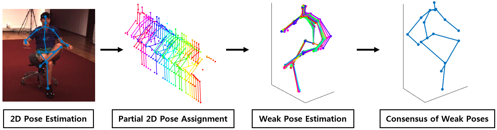
Figure 1: An overview of the proposed method. Given an RGB image, the 2D pose is estimated. After that, each predetermined joint group selects a partial 2D pose input and lifts the partial 2D pose to a partial 3D pose (Different colors mean different joint groups). Finally, the weak reconstructions are aggregated to form the final whole 3D pose.

1 Introduction

In this paper, we deal with the problem of estimating a 3D human pose from a single image, whose objective is to infer the 3D coordinates of the whole body joints given an image. The human pose, which is one of the most valuable information to understand visual data, can be used in many applications, such as human computer interaction, surveilance, augmented reality, video analysis, to name a few. Due to its importance, human pose estimation has been actively researched in computer vision for the last decade [1, 2, 3, 4, 5, 6, 7, 8, 9, 10, 11, 12, 13, 14].

In the early days, people focused on 2D human pose estimation [1, 2, 3, 4, 5] although it is less informative compared to the 3D case. This is because obtaining reasonable 2D estimation results was difficult due to many reasons such as self-occlusions, wild appearance changes, and the high degrees-of-freedom of poses. Early works on 2D pose estimation [1, 2] utilized hand-crafted features like histogram of oriented gradients (HOG) [15], resulting in bad performance. In the meantime, advances in convolutional neural networks (CNN) have made breakthroughs in several computer vision applications, including the 2D human pose estimation problem [3, 4, 5]. By applying CNN to 2D human pose estimation, one can learn rich features that are robust to self-occlusions, in an end-to-end fashion. As a result, one can obtain reasonable 2D estimation results. Here, the performance of the CNN-based estimators has increased as the complexity of the CNN increased.

Recent advances in 2D human pose estimation have promoted the research of 3D human pose estimation. On the other hand, most of the previous approaches have tackled the problem based on an (possibly complicated) estimator that yields a single accurate hypothesis. Unfortunately, the problem is highly ill-posed due to many reasons such as inherent ambiguities of the 3D estimation and self-occlusions. Hence, the complexity of a 3D human pose estimator has been continuously increased to improve accuracy, which would need more and more training samples. However, compared to the case of 2D pose estimation, it is more difficult to collect 3D training samples because a specialized motion capture system is needed. In this light, a single-estimator-based approach may not be the best solution.

Unlike the conventional schemes, we can utilize multiple hypotheses from many different estimators. It is well-known that many complex problems have been successfully handled based on this strategy in computer vision [16, 17]. In this strategy, the final estimation can be obtained robustly by aggregating many “weak” estimations. Here, some of the weak estimations could be bad, and the weak estimator is usually much simpler than the one based on a single estimator.

The complexity of weak estimators can be further reduced if we make them estimate partial hypotheses, i.e., each weak estimator estimates the pose of some partial joints instead of the pose of the whole joints. Actually, the structure of a human body is appropriate to adopt a multiple-partial-hypothesis-based scheme, because the human body is composed of four limbs that could move freely. Here, the four limbs are the left leg, the right leg, the left arm, and the right arm. If each limb is always moved independently, the degrees of freedom for modeling each limb separately would be lower than that of modeling the whole body joints simultaneously. Even if this assumption is not strictly true, we could expect that the degrees of freedom could be reduced by finding a meaningful partial joint groups.

On the other hand, adopting the multiple-partial-hypothesis-based approach to the 3D human pose estimation is not a simple problem. To achieve this, two issues need to be considered. First, we need a proper method of selecting joint groups. Even though there is a chance to reduce the complexity with a multiple-partial-hypothesis-based approach, improper joint groups can ruin the final estimation result. To resolve this, we propose a joint group selection scheme which puts joints that are interdependent to the same joint group. The second issue is about aggregating the weak pose estimations. This is also a difficult problem because there are translation ambiguities between partial poses. Most of regression models assume that the data has a zero mean, and these removed translation components should be revealed before the aggregation. We propose a robust optimization formula which aggregates the weak pose estimations while resolving the translation ambiguity issue.

The main idea of this paper was inspired by [18], which applied the concept of multiple partial hypotheses to the non-rigid structure from motion (NRSfM) problem of which the goal is to reconstruct deforming objects or scenes from their 2D trajectories. NRSfM is in many ways different from 3D pose estimation, most importantly in that NRSfM is a 3D reconstruction problem based on geometric constraints while 3D pose estimation is more of a data-driven machine learning problem. Compared to [18], this work has many novel contributions: (i) It is the first work, to the best of our knowledge, applying the concept of multiple partial hypotheses to 3D pose estimation, and furthermore, it shows the state-of-the-art performance on popular data sets, namely, Human3.6M [19] and HumanEva [20] data sets. (ii) Unlike [18], the proposed scheme can be fine-tuned in an end-to-end fashion, which is beneficial for improving the overall performance. (iii) A domain conversion layer, which transforms heatmap representations to 2D coordinate representations, is proposed for an end-to-end fine-tuning.

2 Related Work

In this section, we introduce related works of single-image-based 3D pose estimation. They are following one of two major trends: (i) a direct regression of 3D human poses from an image [6, 7, 8, 9], and (ii) a two-step approach that first estimates 2D joint coordinates from an image and then infers the 3D pose from the 2D pose [10, 11, 12, 13, 14]. The first approach has an advantage that the entire network could be learned in an end-to-end fashion, which might result in better performance. Chen et al. [6] proposed a method to automatically synthesize images with ground truth 3D poses to handle the issue of insufficient training samples. However, the performance of the 3D pose estimator trained on the synthesized samples was poor on real images, which required an additional domain adaptation process. Rogez et al. [7] also synthesized pairs of images and 3D poses based on 3D motion capture data. Given the synthesized data, they clustered the 3D poses and formulated 3D human pose estimation as a 3D pose classification problem. However, it is hard to guarantee that the synthesized data follows the real-world data distribution. Park et al. [8] proposed an end-to-end network which estimates both 2D pose and relative 3D joint coordinates with respect to multiple root joints directly from a single image. At the test time, they averaged multiple relative 3D joint coordinates to infer the final 3D pose, which can be sensitive to outliers. Pavlakos et al. [9] proposed a different representation for 3D poses other than 3D coordinates. They utilized a voxelized 3D coordinate space for the new 3D representation, and estimated the voxel-wise likelihood of each joint from an image. However, the dimension of the voxel space is too high, which can be a burden in the training process. Furthermore, voxel quantization lowers the resolution of 3D space, which could worsen the performance.

On the other hand, the second approach is a two-step approach that estimates the 2D pose first from an image and then reconstructs the 3D pose from the obtained 2D pose. Yasin et al. [11] and Chen et al. [13] estimated the 2D pose based on a pictorial structure model and a CNN-based model, respectively. After that, the 3D pose is retrieved based on the $k$-nearest neighbor samples of the estimated 2D pose in a ready-made 3D pose database. However, the framework of [11] is based on an iterative procedure that is hard to guarantee the convergence and [13] synthesized a 3D pose database which is hard to ensure that it follows the real-world 3D pose distribution. Chang et al. [12] proposed a conditional-random-field-based model over 2D poses. In the model, the 3D pose is estimated as a byproduct of the inference process. The unary term was defined based on the heatmap of a CNN-based 2D pose estimator, and the prior term was defined based on the consistency of the estimated 2D pose and the reprojected 3D pose. However, the camera parameters are needed to measure the consistency, which limits applicable data. Martinez et al. [14] proposed a fully-connected-layer-based lifting network, applying recent techniques such as residual connections, batch normalization, and a max-norm constraint. The proposed model is quite simple yet shows superior performance. Fang et al. [21] utilized some human body dependencies and relations in the 3D human pose estimation. However, all of the two-step approaches including [14, 21] are difficult to train in an end-to-end fashion, which prevents the potential of future performance improvement.

3 Overview of the propose algorithm

An overview of the proposed method is visualized in Figure 1. In our framework, several joint groups are selected based on the proposed weighted sampling process. The probability distribution is designed to put the joints that have implicit interdependent movements into the same group. After that, each joint group is modeled separately to estimate each partial 3D pose. The proposed joint group selection scheme and the partial 3D pose estimation method for the selected joint groups are introduced in Section 4. Finally, partial 3D poses of the joint groups are aggregated so that the 3D pose of the whole body is estimated based on the proposed robust optimization formula, which is introduces in Section 5.

4 Weak pose estimation

In this section, we will introduce the joint group selection scheme and the 3D pose estimator for a selected joint group. Before explaining the proposed schemes, we introduce some notational conventions. The input RGB image is denoted as $I$, and the 2D human pose is represented by $\mathbf{x}\in\mathbb{R}^{2n}$. Here, $n$ is the total number of body joints and $\mathbf{x}$ is the stack of 2D coordinates of all the joints. Similarly, the 3D human pose is represented by $\mathbf{X}\in\mathbb{R}^{3n}$, which is the stack of 3D coordinates of all the joints. From the $n$ joints, we select some overlapping joint groups. The $j$th joint group is represented as $g_{j}=\{g_{j1},\cdots,g_{jn_{g}}\}$, where the elements of $g_{j}$ are the joint indexes included in the $j$th joint group and $n_{g}$ is the number of joints in a joint group.

4.1 Joint group selection

We design the joint group selection scheme hoping that the complexity of a group pose estimator is lower than a whole-body pose estimator. To realize this expectation, we put joints that are interdependent to the same joint group, and these groups are sampled based on training data. Here, we make use of the fact that most of the training data sets for 3D pose estimation are composed of video sequences, which allows us to use the trajectory information. The interdependency is evaluated based on the similarities of trajectories among joints, where the similarity between the $i$th joint and the $i^{\prime}$th joint is evaluated as

$$s_{ii^{\prime}}\triangleq\sum_{k\in\mathbb{S}}\|\mathbf{X}_{ik}-\mathbf{X}_{i^{\prime}k}\|^{2},$$ (1)

where $\mathbb{S}$ is a sequence of training samples, $\mathbf{X}_{ik}$ and $\mathbf{X}_{i^{\prime}k}$ are the 3D coordinates of the $i$th and the $i^{\prime}$th joint from the $k$th sample, respectively. Based on the similarity measure, the elements of a joint group are sequentially sampled based on a weighted sampling process. The weight of the $i$th joint for the $j$th joint group is defined as

$$\begin{split}w_{i}&\triangleq\left\{\begin{array}[]{ll}\textrm{exp}\left(-\frac{\lambda}{2n_{g}}\sum_{i^{\prime}\in g_{j}}s_{ii^{\prime}}\right),&\text{if }i\notin g_{j},\\ 0,&\text{otherwise,}\end{array}\right.\\ \end{split}$$ (2)

where $\lambda$ is a predefined parameter. Here, the first element of the joint group is selected based on a uniform distribution, and the remaining elements are selected based on the weighted sampling process with the weights $w_{i}$. The joint group selection process is iterated until all the joints are included in joint groups at least $m_{g}$ times. Let $n_{t}$ be the total number of joint groups. Note that the selected joint groups are commonly used for all the samples in a data set.

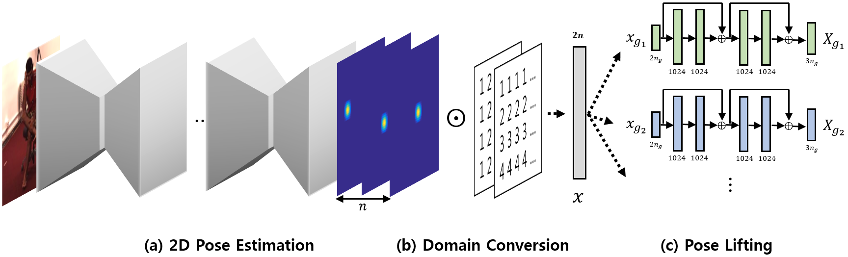
Figure 2: A visualization of the 2D pose estimator network and the 3D pose lifting network. The 2D pose estimator consists of eight hourglass modules, and the output of the network is heatmaps of joints. The 3D pose lifting network consists of fully-connected layers. The input of the 3D pose lifting network is 2D joint coordinates. To apply an end-to-end fine-tuning, we need a differentiable domain conversion layer which is introduced in Section 6.

4.2 Group pose estimation

In this section, we explain the 3D pose estimation scheme for the joint groups. Here, we consider two cases, following the general practice in the literature [10, 14]: (i) estimating 3D poses when the ground truth 2D poses are given (“Case 1”), and (ii) estimating 3D poses when only RGB images are given without any ground truth 2D poses (“Case 2”).

Case 1.  In this case, all we need to do is lifting the given 2D poses to the corresponding 3D poses. This task can be expressed as

$$\mathbf{\hat{X}}_{g_{j}}=f_{j}(\mathbf{x}_{g_{j}}),$$ (3)

where $\mathbf{\hat{X}}_{g_{j}}$ is the estimated 3D pose vector of the $j$th joint group, $\mathbf{x}_{g_{j}}$ is the ground truth 2D pose vector of the $j$th joint group, and $f_{j}$ is the 3D pose lifter for the $j$th joint group. For this task, we could adopt any kinds of 3D lifter as $f_{j}$, though we choose a 3D lifter that is lightweighted and shows good performance. In particular, the network size is important to our approach in respect of efficiency, because there are several joint groups to be lifted. With these considerations in mind, we choose [14], whose complexity is relatively small even though it shows the state-of-the-art performance, for a pose lifter.

The chosen pose lifter [14] is designed based on a neural network. A visualization of the lifting networks is shown in Figure 2(c). The input of the network is the $2n_{g}$-dimensional partial 2D pose vector of a selected joint group. The input is transformed to a $1024$-dimensional vector with a fully-connected layer, which is fed into a fully-connected network which consists of two cascaded blocks. Each block has two consecutive fully-connected layers. After each fully-connected layer, a batch normalization layer, a ReLU activation layer, and a dropout layer are followed. The output of the fully-connected network is a $1024$-dimensional vector, which is again transformed to a $3n_{g}$-dimensional partial 3D pose vector based on another fully-connected layer. For the detailed structure of the network, please refer to [14]. Here, we found out that using a Leaky ReLU activation layer instead of the ReLU activation layer enhances the performance, therefore, we have changed the activation layers of the chosen 3D pose lifter accordingly.

From (3), we derive a loss function for the 3D lifter as

$$L_{\textrm{lifting}}=\sum_{k}\sum_{j}\|\mathbf{X}_{g_{j}}^{k}-f_{j}(\mathbf{x}_{g_{k}}^{k})\|_{F}^{2},$$ (4)

where $\mathbf{X}_{g_{j}}^{k}$ and $\mathbf{x}_{g_{j}}^{k}$ are the ground truth 3D poses and the ground truth 2D poses of the $j$th joint group in the $k$th training sample, respectively. Note here that each joint group has its own pose lifter. Alternatively, we might train a single pose lifter to handle all of the joint groups. However, it is obvious that this approach is worse than using a different lifter for each group, as we have confirmed empirically in Appendix.

Case 2.  In this case, we use the two-step approach which first detects a 2D pose $\mathbf{x}$ from the image $I$ and lifts the 2D pose $\mathbf{x}$ to a 3D pose $\mathbf{X}$. The process of the latter step is the same as that of “Case 1”. Therefore, we only need the part to estimate the 2D pose from the input image. A thing to note here is that most of the high-performance 2D pose estimators output the results in heatmaps. Considering this, the 2D pose estimation step can be expressed as

$$M(\mathbf{\hat{x}})=h(I),$$ (5)

where $\mathbf{\hat{x}}$ is the estimated 2D pose vector, $h$ is the 2D pose estimator, and $M$ is a mapping function which converts 2D joint coordinates to their corresponding heatmaps.

Similar to the 3D pose lifter, we can adopt any kinds of estimator for the 2D pose estimator $h$. Since the accuracy of the 2D pose is very crucial for 3D lifting performance, we choose a state-of-the-art 2D human pose estimator [5]. A visualization of the selected 2D pose estimator is shown in Figure 2(a). It consists of eight cascaded hourglass modules, and each hourglass module consists of successive max-pooling layers and up-sampling layers. Before each max-pooling or up-sampling layer, there is a residual module. The output of the last hourglass module is fed into a $1$x$1$ convolution layer, which results in the heatmaps of the estimated 2D joint positions. Here, we empirically found out that adding a sigmoid layer to the output of the estimator facilitates the training process. Hence, we have added this modification to the estimator. The mapping function $M$ in [5] converts the 2D joint coordinates to $64\times 64$-size heatmaps of which the value represents a Gaussian distribution where the mean is a joint position and the variance is $3$. From (5), a loss function for the 2D pose estimation can be given as

$$L_{\textrm{2d}}=\sum_{k}\sum_{i}\|M(\mathbf{x}_{i}^{k})-h_{i}(I_{k})\|_{F}^{2},$$ (6)

where $I_{k}$ is the RGB image of the $k$th sample, $h_{i}$ is the heatmap of the $i$th joint that is estimated based on $h$, and $\mathbf{x}_{i}^{k}$ is the ground truth 2D coordinates of the $i$th joint in the $k$th sample.

After estimating the heatmap of each joint, the 2D position is obtained based on the proposed domain conversion layer which will be introduced in Section 6. The estimated 2D position from each heatmap is concatenated to form $\mathbf{\hat{x}}$. For the 2D pose estimation process, we use a single estimator, i.e., it is not separately designed for each joint group, because correlations among joints are more important in 2D pose estimation, unlike in the 3D lifter.

5 Consensus of joint groups

So far, joint groups have been selected, and the corresponding partial 3D poses have been estimated. At the test time, partial 3D poses are aggregated to estimate the whole 3D pose based on the proposed robust optimization formula introduced in this section. Before explaining the proposed scheme, we introduce some additional notations. For a 3D pose vector $\mathbf{A}\in\mathbb{R}^{3n}$, $\mathbf{A}|_{g_{j}}\in\mathbb{R}^{3n_{g}}$ indicates the subvector of $\mathbf{A}$, which consists of 3D coordinates of joints that are included in the set $g_{j}$, and $\mathbf{A}^{\prime}\in\mathbb{R}^{n\times 3}$ is a matrix whose rows are filled with the 3D coordinates of $\mathbf{A}$.

There are two issues to consider when designing the aggregation process, which are the translation ambiguities between the estimations and the possibility of poor estimations in some joint groups. The first issue could be resolved based on the fact that there are overlapping joints between the joint groups, i.e., we could reveal the translations with the constraints that the coordinates of the overlapping joints should be the same. To deal with the second issue, we adopt the median statistic that is robust to outliers. It is well-known that we can obtain the median with an $l_{1}$-norm minimization problem. Keeping these in mind, we formulate the following problem:

$$\mathbf{X}=\textrm{argmin}_{\mathbf{X},\mathbf{t}_{j}}\sum_{j}\|\mathbf{X|}_{g_{j}}-\mathbf{\hat{X}}_{g_{j}}-\mathbf{1}\otimes\mathbf{t}_{j}\|_{1},$$ (7)

where $\mathbf{1}$ is the vector of ones, $\otimes$ is the Kronecker product, $\|\cdot\|_{1}$ is the $l_{1}$-norm, and $\mathbf{t}_{j}$ is a $3$-dimensional vector which represents the translation component of the $j$th joint group. Note that this formulation does not evaluate the error of a 3D point isotropically, because the $l_{1}$-norm handles each coordinate independently. Instead, we can incorporate the group sparsity to resolve this issue. Accordingly, the formulation is modified as

$$\mathbf{X}^{\prime}=\textrm{argmin}_{\mathbf{X}^{\prime},\mathbf{t}_{j}}\sum_{j}\|\mathbf{X^{\prime}|}_{g_{j}}-\mathbf{X}^{\prime}_{g_{j}}-\mathbf{1}\otimes\mathbf{t}_{j}^{T}\|_{2,1},$$ (8)

where $\|\cdot\|_{2,1}$ is the $l_{2,1}$-norm. This can also be expressed as

$$(\mathbf{X}^{\prime},t)=\textrm{argmin}_{\mathbf{X}^{\prime},\mathbf{t}}\left\|\begin{bmatrix}\mathbf{E}~{}~{}&\mathbf{I}\otimes\mathbf{1}\end{bmatrix}\begin{bmatrix}\mathbf{X}^{\prime}\\ \mathbf{t}\end{bmatrix}-\mathbf{F}\right\|_{2,1},$$ (9)

where $\mathbf{I}$ is the identity matrix, and $\mathbf{E}$, $\mathbf{F}$, and $\mathbf{t}$ are defined as

$$\begin{split}\mathbf{E}=\begin{bmatrix}\mathbf{E}_{1},&\mathbf{E}_{2},&\cdots\end{bmatrix}^{T},~{}~{}\mathbf{F}=\begin{bmatrix}\mathbf{X}^{\prime}_{g_{1}},&\mathbf{X}^{\prime}_{g_{2}},&\cdots\end{bmatrix}^{T},~{}~{}\mathbf{t}=\begin{bmatrix}\mathbf{t}_{1},&\mathbf{t}_{2},&\cdots\end{bmatrix}^{T}.\end{split}$$ (10)

Here, $\mathbf{E}_{j}$ is an $n\times n_{g}$ matrix each of whose columns is a one-hot column vector that represents the index of each joint in the $j$th joint group.

This problem can be solved with the alternating directional method of multipliers (ADMM) [22], with an auxiliary variable $\mathbf{N}$. The problem is modified as

$$(\mathbf{G},\mathbf{N})=\textrm{argmin}_{\mathbf{G},\mathbf{N}}\frac{\mu}{2}\|\mathbf{N}-\begin{bmatrix}\mathbf{E}~{}~{}&\mathbf{I}\otimes\mathbf{1}\end{bmatrix}\mathbf{G}+\mathbf{F}\|_{F}^{2}+\|\mathbf{N}\|_{2,1},$$ (11)

where $\mathbf{G}\triangleq\begin{bmatrix}\mathbf{X}^{\prime},\mathbf{t}\end{bmatrix}^{T}$, and $\mu$ is a parameter. The solution of this problem can be obtained by solving $\mathbf{G}$ and $\mathbf{N}$ alternatively until convergence. Note here that both $\mathbf{G}$ and $\mathbf{N}$ have closed-form solutions based on a pseudo-inverse operation and a soft-thresholding operation, respectively.

6 End-to-end learning for fine-tuning

We have introduced a two-step algorithm for 3D human pose estimation. However, there is a chance to improve the overall performance if we fine-tune the whole framework in an end-to-end fashion. In this section, we will introduce how this is possible.

Consensus cost.  In the proposed two-step algorithm, the 3D lifting network of each joint group has been trained separately. However, we can add a loss of aggregation to the objective function of the 3D lifting network, to improve the overall performance further. The aggregation cost is defined as

$$L_{\textrm{aggre}}=\sum_{j}\|\mathbf{X|}_{g_{j}}\mathbf{W}_{j}-\mathbf{\hat{X}}_{g_{j}}\|_{F}^{2},$$ (12)

where $\mathbf{W}_{j}\triangleq\mathbf{I}-\frac{\mathbf{w}_{j}\mathbf{w}_{j}^{T}}{n_{g}}$, and $\mathbf{w}_{j}$ is the $n$-dimensional vector of which the element is $1$ if it is included in the $j$th joint group and $0$ otherwise. Here, the role of $\mathbf{W}_{j}$ is selecting the components of the $j$th joint group with removing the translation component. The exact translation of (7) to the aggregation loss is to use an $l_{2,1}$-norm version of (12), but we empirically found out that the $l_{2,1}$-norm unstabilizes the backpropagation process. Hence, we instead use the square of the Frobenius norm in the aggregation loss.

Domain conversion.  The outputs of the 2D pose estimator are heatmaps of joints, and the inputs of the 3D lifters are 2D joint coordinates. Hence, for an end-to-end training, we need a layer which converts the heatmaps to 2D coordinates. An argmax layer could carry out this role in the forward pass, but it blocks the back-propagation of gradients in the training process since the argmax operation is not differentiable. To resolve this, we propose a novel differentiable domain conversion layer. Before proposing the conversion layer, we introduce additional notations. Let $[a:b]$ be a $(b-a+1)$-dimensional vector of which the elements are monotonically increasing integers from $a$ to $b$, and let $\tilde{h}_{i}(I)$ be a normalized version of $h_{i}(I)$ so that the sum of all values becomes one. The heatmap of the $i$th joint in the $k$th sample is converted to 2D coordinates as

$$x_{i}=\sum_{p}\sum_{q}\big{[}\tilde{h}_{i}(I_{k})\odot([1:l_{x}]\otimes\mathbf{1}^{T})\big{]}_{(p,q)},~{}~{}y_{i}=\sum_{p}\sum_{q}\big{[}\tilde{h}_{i}(I_{k})\odot(\mathbf{1}\otimes[1:l_{y}]^{T})\big{]}_{(p,q)},$$ (13)

where $l_{x}$ and $l_{y}$ are the width and height of the heatmap, respectively, $\odot$ is the Hadamard product, $\otimes$ is the Kronecker product, and $\big{[}\mathbf{A}\big{]}_{(p,q)}$ is the $(p,q)$-th element of $\mathbf{A}$. Note that the proposed layer only consists of linear operations, which are differentiable. A possible downside of this approach is that the outputs of the proposed layer may be different from those of an argmax layer, i.e., there might be a bias between the two. However, we empirically found out that there is only a slight difference, as shown in Appendix.

Fine-tuning procedure.  We empirically found out that training the whole framework from the scratch results in a bad local optimum with poor performance. Hence, we pre-train the 2D pose estimator and the 3D lifter based on the loss functions $L_{\textrm{2d}}$ and $L_{\textrm{lifting}}+L_{\textrm{aggre}}$, respectively. After that, we fine-tune the whole network in an end-to-end fashion with the following loss function:

$$L_{\textrm{e2e}}=\alpha L_{\textrm{2d}}+L_{\textrm{lifting}}+L_{\textrm{aggre}},$$ (14)

where $\alpha$ is a weighting parameter.

Table 1: Performance comparison results on the Human3.6M data set in “Case 1” with “Protocol 1.” Here, $n_{g}$ and $n_{t}$ are the number of joints included in a joint group and the total number of joint groups, respectively.

Protocol 1	Direct.	Discuss	Eating	Greet	Phone	Photo	Pose	Purch.	Sitting	SittingD	Smoke	Wait	WalkD	Walk	WalkT	Avg
Martinez et al. [14]	37.7	44.4	40.3	42.1	48.2	54.9	44.4	42.1	54.6	58.0	45.1	46.4	47.6	36.4	40.4	45.5
Ours ($n_{g}=8$)	36.0	41.0	39.2	41.3	42.7	60.3	42.2	41.9	56.2	49.9	41.9	42.2	44.6	40.2	33.7	43.4
Ours ($n_{g}=10$)	33.9	40.5	34.8	38.6	40.4	50.2	41.0	39.8	55.4	48.8	39.4	40.4	42.3	36.5	31.9	40.9
Ours ($n_{g}=13$)	34.5	41.7	35.4	39.4	41.2	50.9	41.4	40.9	56.0	47.8	40.0	41.1	43.7	35.6	32.6	41.5
Ours ($n_{g}=15$)	35.3	42.6	37.1	39.9	43.3	52.1	42.8	40.5	55.9	50.5	41.4	41.9	44.3	36.0	32.4	42.6
Ours ($n_{g}=17$)	35.0	42.4	37.0	39.7	43.7	52.7	42.2	39.8	56.3	51.1	41.7	41.4	45.1	35.0	32.1	42.6
Ours ($n_{g}=17$, $n_{t}=1$)	36.0	43.3	37.4	40.3	44.2	53.4	42.7	40.7	56.4	52.1	42.5	42.4	45.5	35.5	32.6	43.3

Table 2: Performance comparison results on the Human3.6M data set in “Case 2” with “Protocol 1.”

Protocol 1	Direct.	Discuss	Eating	Greet	Phone	Photo	Pose	Purch.	Sitting	SittingD	Smoke	Wait	WalkD	Walk	WalkT	Avg
LinKDE [19]	132.7	183.6	132.3	164.4	162.1	205.9	150.6	171.3	151.6	243.0	162.1	170.7	177.1	96.6	127.9	162.1
Li et al [23]	-	136.9	96.9	124.7	-	128.7	-	-	-	-	-	-	132.2	70.0	-	-
Tekin et al [24]	102.4	147.2	88.8	125.3	118.0	182.7	112.4	129.2	138.9	224.9	118.4	138.8	126.3	55.1	65.8	125.0
Zhou et al [10]	87.4	109.3	87.1	103.2	116.2	143.3	106.9	99.8	124.5	199.2	107.4	118.1	114.2	79.4	97.7	113.0
Tekin et al [25]	-	129.1	91.4	121.7	-	162.2	-	-	-	-	-	-	130.5	65.8	-	-
Ghezelghieh et al [26]	80.3	80.4	78.1	89.7	-	-	-	-	-	-	-	-	-	95.1	82.2	-
Du et al [27]	85.1	112.7	104.9	122.1	139.1	135.9	105.9	166.2	117.5	226.9	120.0	117.7	137.4	99.3	106.5	126.5
Park et al [8]	100.3	116.2	90.0	116.5	115.3	149.5	117.6	106.9	137.2	190.8	105.8	125.1	131.9	62.6	96.2	117.3
Zhou et al [28]	91.8	102.4	96.7	98.8	113.4	125.2	90.0	93.8	132.2	159.0	107.0	94.4	126.0	79.0	99.0	107.3
Pavlakos et al [9]	67.4	71.9	66.7	69.1	72.0	77.0	65.0	68.3	83.7	96.5	71.7	65.8	74.9	59.1	63.2	71.9
Martinez et al [14]	51.8	56.2	58.1	59.0	69.5	78.4	55.2	58.1	74.0	94.6	62.3	59.1	65.1	49.5	52.4	62.9
Fang et al [21]	50.1	54.3	57.0	57.1	66.6	73.3	53.4	55.7	72.8	88.6	60.3	57.7	62.7	47.5	50.6	60.4
Ours	48.4	52.9	55.2	53.8	62.8	73.3	52.3	52.2	71.0	89.9	58.2	53.6	61.0	43.2	50.0	58.8

7 Experimental results

We have evaluated the proposed scheme quantitatively and qualitatively on several data sets. For the quantitative experiments, we applied the proposed scheme on popular benchmark data sets, namely the Human3.6M [19] data set and the HumanEva-I [20] data set. We also applied the proposed scheme on the MPII data set [29] for the qualitative evaluation.

Human3.6M is the largest data set, to the best of our knowledge, that has synchronized RGB images and the corresponding 3D joint coordinates. Intrinsic and extrinsic camera parameters are also provided so that we can obtain the corresponding 2D joint coordinates. It consists of $15$ actions (e.q., direction, discussion, eating, etc.), and every action is performed by $7$ actors. Each demonstration is captured in $4$ different angles simultaneously. Following the standard practices in the literature [14, 21], the demonstrations of subjects $1$, $5$, $6$, $7$, and $8$ were used as the training set, and the demonstrations of subjects $9$ and $11$ were used as the test set.

HumanEva-I is a smaller data set compared to the Human3.6M data set. It also has synchronized RGB images with the corresponding 3D joint coordinates and 2D joint coordinates. Following the practices in [11, 9, 14], we evaluated on all subjects, separately in each action.

MPII is a popular benchmark data set for 2D pose estimation, which has RGB images taken “in the wild” and the corresponding manually-annotated ground truth 2D joint coordinates. It has no ground truth 3D poses.

We have compared the performance of the proposed scheme based on the Euclidean distance between the ground truth 3D coordinate and the inferred 3D coordinates after an alignment. The final performance is the average distance of all joints and test samples. In the literature [14, 21], two types of alignment methods have been used, therefore, we report the performance in both the cases. In the first case, the average distances are measured after the root joint alignments between the ground truth 3D poses and the inferred 3D poses, and we call this “Protocol 1”. In the second case, the average distances are measured after a rigid alignment, and we call this “Protocol 2”. For all the experiments, we used the following parameter setting unless we notice: $m_{g}=10$, $\lambda=10$, $\alpha=100$, $n_{g}=n-1$, and we used the first sequence of the training set as $\mathbb{S}$.

Table 3: Performance comparison results on the Human3.6M data set in “Case 2” with “Protocol 2.”

Protocol 2	Direct.	Discuss	Eating	Greet	Phone	Photo	Pose	Purch.	Sitting	SittingD	Smoke	Wait	WalkD	Walk	WalkT	Avg
Akhter et al. [30]	199.2	177.6	161.8	197.8	176.2	186.5	195.4	167.3	160.7	173.7	177.8	181.9	176.2	198.6	192.7	181.1
Ramakrishna et al. [31]	137.4	149.3	141.6	154.3	157.7	158.9	141.8	158.1	168.6	175.6	160.4	161.7	150.0	174.8	150.2	157.3
Zhou et al. [32]	99.7	95.8	87.9	116.8	108.3	107.3	93.5	95.3	109.1	137.5	106.0	102.2	106.5	110.4	115.2	106.7
Bogo et al. [33]	62.0	60.2	67.8	76.5	92.1	77.0	73.0	75.3	100.3	137.3	83.4	77.3	86.8	79.7	87.7	82.3
Moreno-Noguer [34]	66.1	61.7	84.5	73.7	65.2	67.2	60.9	67.3	103.5	74.6	92.6	69.6	71.5	78.0	73.2	74.0
Pavlakos et al [9]	-	-	-	-	-	-	-	-	-	-	-	-	-	-	-	51.9
Martinez et al [14]	39.5	43.2	46.4	47.0	51.0	56.0	41.4	40.6	56.5	69.4	49.2	45.0	49.5	38.0	43.1	47.7
Fang et al [21]	38.2	41.7	43.7	44.9	48.5	55.3	40.2	38.2	54.5	64.4	47.2	44.3	47.3	36.7	41.7	45.7
Ours	39.6	41.7	45.2	45.0	46.3	55.8	39.1	38.9	55.0	67.2	45.9	42.0	47.0	33.1	40.5	45.7

7.1 Implementation details

We used a separate 2D pose estimator on each data set, namely, the Human3.6M and the HumanEva-I data sets. Both the 2D pose estimators were pre-trained on the MPII data set for $100$ epochs using RMSProp [35]. We used an exponentially-decaying learning rate with a starting learning rate of $2.5\times 10^{-4}$. After that, we fine-tuned the estimators for $20$ epochs using RMSProp with the same starting learning rate which was reduced by the factor of $5$ after $10$ epochs. In each training process, we used the batch size of $64$. Here, in the fine-tuning process on Human3.6M, we uniformly sub-sampled the data set with the factor of $50$.

We also trained 3D pose lifters separately on each data set. The 3D pose lifters were also trained based on RMSProp with an exponentially-decaying learning rate with a starting learning rate of $0.001$. On the Human3.6M data set, the 3D pose lifter was trained for $100$ epochs with the batch size of $1024$. On the other hand, because the number of training samples on HumanEva-I is smaller than $1024$, we used a smaller batch size of $64$, which was trained for $500$ epochs. Here, the 3D pose lifter network was trained with the estimation results from each 2D pose estimator as input.

The whole framework was fine-tuned for $5$ epochs using RMSProp, with the batch size of $128$, in an end-to-end fashion as proposed in Section 6. We used exponentially-decaying learning rates of $1.25\times 10^{-4}$ (for the 2D pose estimator) and $0.0005$ (for the 3D pose lifter). It is well-known that the first part of a network captures universal features like edges. Therefore, we fixed the parameters of the first five hourglass modules. In the fine-tuning process on Human3.6M, we uniformly sub-sampled the data set with the factor of $50$ due to the large number of training samples. Another thing to note is that, for HumanEva-I, this end-to-end fine-tuning was not helpful, because the HumanEva-I data set has too small number of training samples, resulting in an overfitting of the whole framework.

Table 4: Performance on the HumanEva-I data set in “Case 2” with “Protocol 2.”

Protocol 2	Walking			Jogging			Avg
	S1	S2	S3	S1	S2	S3
Radwan et al. [36]	75.1	99.8	93.8	79.2	89.8	99.4	89.5
Wang et al. [37]	71.9	75.7	85.3	62.6	77.7	54.4	71.3
Simo-Serra et al. [38]	65.1	48.6	73.5	74.2	46.6	32.2	56.7
Bo et al. [39]	46.4	30.3	64.9	64.5	48.0	38.2	48.7
Kostrikov et al. [40]	44.0	30.9	41.7	57.2	35.0	33.3	40.3
Yasin et al. [11]	35.8	32.4	41.6	46.6	41.4	35.4	38.9
Moreno-Noguer et al. [34]	19.7	13.0	24.9	39.7	20.0	21.0	26.9
Pavlakos et al. [9]	22.1	21.9	29.0	29.8	23.6	26.0	25.5
Martinez et al. [14]	19.7	17.4	46.8	26.9	18.2	18.6	24.6
Fang et al [21]	19.4	16.8	37.4	30.4	17.6	16.3	22.9
Ours	18.1	15.6	31.7	38.2	18.6	17.9	22.5

Table 5: Ablation experiments on different components in our framework. It was performed on the Human3.6M data set in “Case 2” with “Protocol 1”.

Variant	Ours	w/o $L_{\textrm{e2e}}$	w/o $l_{2,1}$	w/o $L_{\textrm{aggre}}$	Random Selection	Random Selection, w/o $L_{\textrm{e2e}}$
Error (mm)	58.8	60.1	58.9	59.4	62.3	64.8
$\triangle$	-	1.3	0.1	0.6	3.5	6.0

7.2 Quantitative evaluation

Case 1.  We compared the performance of the proposed method to that of [14] on Human3.6M data set, in the case that the ground truth 2D poses are given. In this experiment, we used “Protocol 1” for the evaluation, and the results are summarized in Table 1. Here, we report the performance with various values of $n_{g}$. In all the cases, the proposed scheme shows superior performance to [14]. In the result, we can confirm the effectiveness of the proposed multiple-partial-hypothesis-based approach. As $n_{g}$ decreases from $17$ (the total number of joints) to $10$, the errors are monotonically decreased. This result shows that modeling a partial joint group has a lower complexity compared to modeling full joints. On the other hand, in the case of $n_{g}=17$, i.e., each 3D pose lifter estimates full 3D poses, we can demonstrate the effectiveness of the multiple-hypothesis-based model. Even in the case that each 3D pose lifter estimates full 3D pose, their aggregation has better performance. Finally, in the case of $n_{g}=17$ and $n_{t}=1$, where only a single “weak” 3D lifter is used without combining multiple hypotheses, the proposed method is better than [14]. In this case, since the weak 3D lifter is a modified version of [14], the only difference between the two is the modifications we made. Since our version gives better performance, this justifies the use of such modifications.

Case 2.  We compared the performance of the proposed scheme with various methods [19, 23, 24, 10, 25, 26, 27, 8, 28, 9, 14, 21, 30, 31, 32, 33, 34] in the case that only RGB images are given without any ground truth 2D poses on the Human3.6M data set. The comparison results based on “Protocol 1” and “Protocol 2” are shown in Table 2 and Table 3, respectively. In the case of “Protocol 1”, the proposed method shows the state-of-the-art performance. On the other hand, for “Protocol 2”, the proposed scheme shows almost the same performance with [21] on average. However, since “Protocol 2” needs a rigid alignment, we claim that the proposed method has better performance. We also compared the performance of the proposed method on the HumanEva-I data set with various methods [36, 37, 38, 39, 40, 11, 34, 9, 14, 21]. The result is summarized in Table 4. The proposed method shows the best average performance, which demonstrates the effectiveness of the proposed framework.

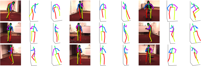
Figure 3: 3D estimation results of some examples in the test set of the Human36M data set. Left: Input RGB images and the corresponding 2D pose estimations. Middle, Right: 3D pose estimation results in two different views.

Figure 4: Some examples in the test set of the MPII data set. Left: Input RGB images and the corresponding 2D pose estimations. Middle, Right: 3D pose estimation results in two different views.

7.3 Ablation experiments

We performed some ablation experiments on the Human3.6M data set with “Protocol 1”. The performance was evaluated with removing some components of the proposed framework. The results are summarized in Table 5. Removing the end-to-end fine-tuning process increased the error by 1.3mm. The error was increased by 0.1mm when we performed the aggregation process with the $l_{1}$-norm objective function, and the error was increased by 0.6mm when the aggregation loss $L_{\textrm{aggre}}$ was not included in the loss function. In the mean time, when we randomly selected joint groups without using the proposed selecting scheme, the error was increased by 3.5mm, and removing the end-to-end fine-tuning process further increased the error by 2.5mm.

7.4 Qualitative evaluation

We report some qualitative results on the Human3.6M and the MPII data sets. Some results on Human3.6M are visualized in Figure 3, and those on MPII are visualized in Figure 4. Note that the MPII data set has no ground truth 3D poses, hence, for this data set, we used the proposed network trained on the Human3.6M data set. Unlike the images of Human3.6M, those of MPII are taken “in the wild.” Although the proposed scheme was not trained on the wild images, we can see that the estimation results are reasonable. More results are available in Appendix.

8 Conclusion

In this paper, we dealt with the problem of 3D human pose estimation from a single image. Single-image-based 3D human pose estimation is a very tough problem due to many reasons such as self-occlusions, wild appearance changes, and inherent ambiguities of 3D estimation from a 2D cue. Most of the conventional methods have handled the problem with a single complex estimator, which have become requiring increasingly complex estimators to enhance the performance. In this paper, we proposed a multiple-partial-hypothesis-based framework for the problem. We selected joint groups from the data based on the proposed sampling scheme, and estimated partial 3D poses of joint groups separately. These were later aggregated to obtain the final full 3D pose using the proposed robust optimization formula. The proposed method is fine-tuned in an end-to-end fashion, resulting in better performance. In the experiments, the proposed framework shows the state-of-the-art performance on the popular benchmark data sets. The proposed framework can be successfully adopted to a more general problem like multi-person 3D pose estimation based on a properly-designed joint-group selection scheme, which is left as a future work.

A Appendix

A.1 A single 3D pose lifter for all joint groups

We introduce the performance of the proposed scheme in case we train a single pose lifter to handle all joint groups. We have compared the results of training separate 3D pose lifters to those of training a single pose lifter on the Human3.6M data set [19] in “Case 1” with “Protocol 1”. The results are summarized in Table 6. The performance of the modified scheme is much worse than that of the original scheme proposed in the paper, which confirms the effectiveness of training a separate 3D pose lifter for each joint group.

Table 6: Performance comparison results on the Human3.6M data set in “Case 1” with “Protocol 1”. ‘Single’ means that we trained a single pose lifter to handle all of the joint groups.

Protocol 1	Direct.	Discuss	Eating	Greet	Phone	Photo	Pose	Purch.	Sitting	SittingD	Smoke	Wait	WalkD	Walk	WalkT	Avg
Ours ($n_{g}=10$)	33.9	40.5	34.8	38.6	40.4	50.2	41.0	39.8	55.4	48.8	39.4	40.4	42.3	36.5	31.9	40.9
Ours ($n_{g}=10$, Single)	132.1	155.2	172.4	147.2	182.5	176.2	126.3	183.3	225.8	195.7	165.3	145.6	174.2	149.3	147.5	165.9
Ours ($n_{g}=13$)	34.5	41.7	35.4	39.4	41.2	50.9	41.4	40.9	56.0	47.8	40.0	41.1	43.7	35.6	32.6	41.5
Ours ($n_{g}=13$, Single)	94.4	106.5	127.0	107.2	123.3	130.4	93.0	119.9	157.7	147.2	118.0	102.7	123.6	102.0	94.9	117.1
Ours ($n_{g}=15$)	35.3	42.6	37.1	39.9	43.3	52.1	42.8	40.5	55.9	50.5	41.4	41.9	44.3	36.0	32.4	42.6
Ours ($n_{g}=15$, Single)	82.2	82.0	88.6	92.7	78.8	112.0	77.5	87.5	107.3	91.9	79.4	80.8	93.5	85.0	76.6	86.7

A.2 Bias analysis of the domain conversion layer

We have proposed a novel domain conversion layer which transforms a heatmap to its 2D coordinate in the paper. The proposed domain conversion layer consists of differentiable linear operations, which allows the back-propagation of gradients in the training process. However, there might be a bias between the output of the domain conversion layer and that of the corresponding argmax layer. In an ideal case that the mean and the peak of the heatmap distribution coincide, we can verify that there is no bias between the two. Note that a 2D pose estimator is trained based on a ground truth heatmap, of which its normalized distribution is a Gaussian distribution. Let us assume that, in an ideal case, the actual (normalized) output heatmap of the $i$th joint is a Gaussian distribution which is described as

$$\begin{split}\big{[}\tilde{h}_{i}(I_{k})\big{]}_{(p,q)}&=\frac{\textrm{exp}\left(-\frac{1}{2\sigma^{2}}\left((p-x_{i})^{2}+(q-y_{i})^{2})\right)\right)}{\sqrt{(2\pi\sigma^{2})^{2}}}\triangleq\mathbf{N}_{x,y}(p,q)\\ &=\frac{\textrm{exp}\left(-\frac{1}{2\sigma^{2}}\left(p-x_{i}\right)^{2}\right)}{\sqrt{2\pi\sigma^{2}}}\cdot\frac{\textrm{exp}\left(-\frac{1}{2\sigma^{2}}\left(q-y_{i}\right)^{2}\right)}{\sqrt{2\pi\sigma^{2}}}\\ &\triangleq\mathbf{N}_{x}(p)\mathbf{N}_{y}(q),\end{split}$$ (15)

where $x_{i}$ and $y_{i}$ are the 2D coordinates of the $i$th joint, and $\sigma^{2}$ is the variance of the Gaussian distribution. We can verify that the proposed domain conversion layer provides an unbiased 2D coordinates from its ground truth heatmap as

$$\begin{split}&\sum_{p}\sum_{q}\big{[}\tilde{h}_{i}(I_{k})\odot([1:l_{x}]\otimes\mathbf{1}^{T})\big{]}_{(p,q)}=\sum_{p}\sum_{q}\big{[}\tilde{h}_{i}(I_{k})\big{]}_{(p,q)}\cdot q\\ &=\sum_{p}\sum_{q}\mathbf{N}_{x,y}(p,q)\cdot q=\sum_{p}\sum_{q}\mathbf{N}_{x}(p)\mathbf{N}_{y}(q)\cdot q\\ &=\sum_{p}\mathbf{N}_{x}(p)\sum_{q}\mathbf{N}_{y}(q)\cdot q=x_{i}.\end{split}$$ (16)

We can verify a similar relation for $y_{i}$.

In reality, we cannot expect to have such an ideal output distribution from a 2D pose estimator. In this case, there might be a bias between the output of the proposed domain conversion layer and that of the corresponding argmax layer. However, we empirically found out that there is only a slight difference. We empirically calculated the biases on the test samples of the Human3.6M data set, based on the proposed framework trained on the same data set. In this process, we sub-sampled the test set by the factor of $5$ due to the large sample size, and the biases were evaluated on the $64\times 64$-size heatmaps. Based on these bias samples, we performed nonparametric estimations to find their underlying probability density for each joint based on a normal kernel function. The results are shown in Figure 5. We can verify that the norms of the biases are mostly less than a pixel, which is a slight difference considering the performance improvement based on the proposed end-to-end fine-tuning process.

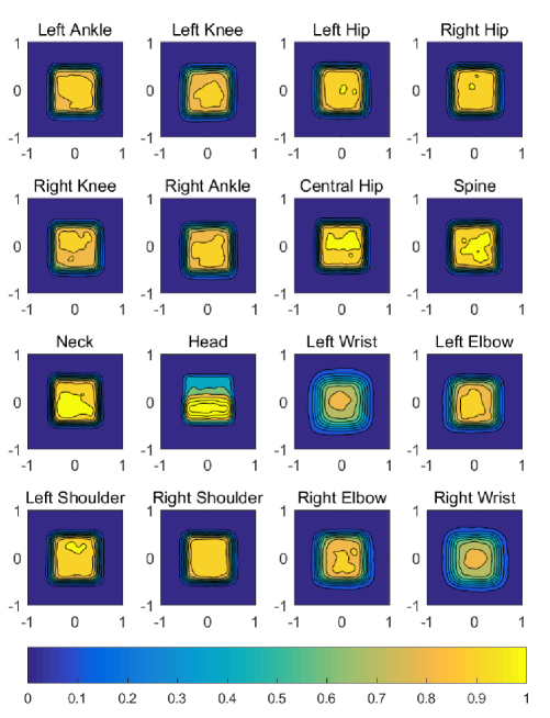
Figure 5: A visualization of the estimated probability density of the biases for each joint.

A.3 Qualitative examples

We present some more qualitative results in this section. Some results on the Human3.6M data set are visualized in Figure 6, and those on the MPII data set [29] are visualized in Figure 7. We can confirm that the proposed framework successfully estimates a 3D pose from an image.

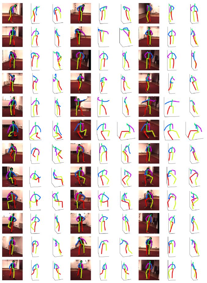
Figure 6: 3D estimation examples for the test samples of the Human3.6M data set. Left: Input RGB images and the corresponding 2D pose estimations. Middle, Right: 3D pose estimation results in two different views.

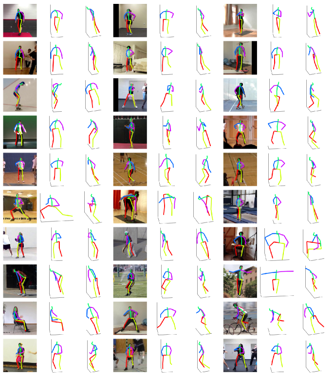
Figure 7: 3D estimation examples for the test samples of the MPII data set. Left: Input RGB images and the corresponding 2D pose estimations. Middle, Right: 3D pose estimation results in two different views.

References

- [1] Bourdev, L., Malik, J.: Poselets: Body part detectors trained using 3D human pose annotations. In: Proc. of the IEEE International Conference on Computer Vision. (2009) 1365–1372
- [2] Yang, Y., Ramanan, D.: Articulated human detection with flexible mixtures of parts. IEEE Transactions on Pattern Analysis and Machine Intelligence 35(12) (2013) 2878–2890
- [3] Toshev, A., Szegedy, C.: Deeppose: Human pose estimation via deep neural networks. In: Proc. of the IEEE Computer Vision and Pattern Recognition. (2014)
- [4] Wei, S.E., Ramakrishna, V., Kanade, T., Sheikh, Y.: Convolutional pose machines. In: Proc. of the IEEE Computer Vision and Pattern Recognition. (2016)
- [5] Newell, A., Yang, K., Deng, J.: Stacked hourglass networks for human pose estimation. In: Proc. of the European Conference on Computer Vision. (2016) 483–499
- [6] Chen, W., Wang, H., Li, Y., Su, H., Wang, Z., Tu, C., Lischinski, D., Cohen-Or, D., Chen, B.: Synthesizing training images for boosting human 3D pose estimation. In: Proc. of the IEEE International Conference on 3D Vision. (2016) 479–488
- [7] Rogez, G., Schmid, C.: Mocap-guided data augmentation for 3D pose estimation in the wild. In: Advances in Neural Information Processing Systems. (2016) 3108–3116
- [8] Park, S., Hwang, J., Kwak, N.: 3D human pose estimation using convolutional neural networks with 2D pose information. In: Proc. of the European Conference on Computer Vision Workshops. (2016) 156–169
- [9] Pavlakos, G., Zhou, X., Derpanis, K.G., Daniilidis, K.: Coarse-to-fine volumetric prediction for single-image 3D human pose. In: Proc. of the IEEE Computer Vision and Pattern Recognition. (2017) 1263–1272
- [10] Zhou, X., Zhu, M., Leonardos, S., Derpanis, K.G., Daniilidis, K.: Sparseness meets deepness: 3D human pose estimation from monocular video. In: Proc. of the IEEE Computer Vision and Pattern Recognition. (2016) 4966–4975
- [11] Yasin, H., Iqbal, U., Kruger, B., Weber, A., Gall, J.: A dual-source approach for 3D pose estimation from a single image. In: Proc. of the IEEE Computer Vision and Pattern Recognition. (2016) 4948–4956
- [12] Chang, J.Y., Lee, K.M.: 2D-3D pose consistency-based conditional random fields for 3D human pose estimation. arXiv preprint arXiv:1704.03986 (2017)
- [13] Chen, C.H., Ramanan, D.: 3D human pose estimation= 2D pose estimation+ matching. In: Proc. of the IEEE Computer Vision and Pattern Recognition. (2017) 7035–7043
- [14] Martinez, J., Hossain, R., Romero, J., Little, J.J.: A simple yet effective baseline for 3d human pose estimation. Proc. of the IEEE International Conference on Computer Vision (2017)
- [15] Dalal, N., Triggs, B.: Histograms of oriented gradients for human detection. In: Proc. of the IEEE Computer Vision and Pattern Recognition. (2005) 886–893
- [16] Viola, P., Jones, M.J.: Robust real-time face detection. International Journal of Computer Vision 57(2) (2004) 137–154
- [17] Breiman, L.: Random forests. Machine learning 45(1) (2001) 5–32
- [18] Lee, M., Cho, J., Oh, S.: Consensus of non-rigid reconstructions. In: Proc. of the IEEE Computer Vision and Pattern Recognition. (2016) 4670–4678
- [19] Ionescu, C., Papava, D., Olaru, V., Sminchisescu, C.: Human3.6M: Large scale datasets and predictive methods for 3d human sensing in natural environments. IEEE Transactions on Pattern Analysis and Machine Intelligence 36(7) (2014) 1325–1339
- [20] Sigal, L., Balan, A.O., Black, M.J.: Humaneva: Synchronized video and motion capture dataset and baseline algorithm for evaluation of articulated human motion. International Journal of Computer Vision 87(1) (2010) 4–27
- [21] Fang, H.S., Xu, Y., Wang, W., Liu, X., Zhu, S.C.: Learning pose grammar to encode human body configuration for 3D pose estimation. In: Proc. of the AAAI Conference on Artificial Intelligence. (2018)
- [22] Lin, Z., Chen, M., Ma, Y.: The augmented lagrange multiplier method for exact recovery of corrupted low-rank matrices. arXiv preprint arXiv:1009.5055 (2010)
- [23] Li, S., Zhang, W., Chan, A.B.: Maximum-margin structured learning with deep networks for 3D human pose estimation. In: Proc. of the IEEE International Conference on Computer Vision. (2015) 2848–2856
- [24] Tekin, B., Rozantsev, A., Lepetit, V., Fua, P.: Direct prediction of 3D body poses from motion compensated sequences. In: Proc. of the IEEE Computer Vision and Pattern Recognition. (2016) 991–1000
- [25] Tekin, B., Katircioglu, I., Salzmann, M., Lepetit, V., Fua, P.: Structured prediction of 3D human pose with deep neural networks. Proc. of the British Machine Vision Conference (2016)
- [26] Ghezelghieh, M.F., Kasturi, R., Sarkar, S.: Learning camera viewpoint using cnn to improve 3D body pose estimation. In: Proc. of the IEEE International Conference on 3D Vision. (2016) 685–693
- [27] Du, Y., Wong, Y., Liu, Y., Han, F., Gui, Y., Wang, Z., Kankanhalli, M., Geng, W.: Marker-less 3D human motion capture with monocular image sequence and height-maps. In: Proc. of the European Conference on Computer Vision. (2016) 20–36
- [28] Zhou, X., Sun, X., Zhang, W., Liang, S., Wei, Y.: Deep kinematic pose regression. In: Proc. of the European Conference on Computer Vision. (2016) 186–201
- [29] Andriluka, M., Pishchulin, L., Gehler, P., Schiele, B.: 2D human pose estimation: New benchmark and state of the art analysis. In: Proc. of the IEEE Computer Vision and Pattern Recognition. (2014)
- [30] Akhter, I., Black, M.J.: Pose-conditioned joint angle limits for 3D human pose reconstruction. In: Proc. of the IEEE Computer Vision and Pattern Recognition. (2015) 1446–1455
- [31] Ramakrishna, V., Kanade, T., Sheikh, Y.: Reconstructing 3D human pose from 2D image landmarks. Proc. of the European Conference on Computer Vision (2012) 573–586
- [32] Zhou, X., Zhu, M., Leonardos, S., Daniilidis, K.: Sparse representation for 3D shape estimation: A convex relaxation approach. IEEE Transactions on Pattern Analysis and Machine Intelligence 39(8) (2017) 1648–1661
- [33] Bogo, F., Kanazawa, A., Lassner, C., Gehler, P., Romero, J., Black, M.J.: Keep it smpl: Automatic estimation of 3D human pose and shape from a single image. In: Proc. of the European Conference on Computer Vision. (2016) 561–578
- [34] Moreno-Noguer, F.: 3D human pose estimation from a single image via distance matrix regression. Proc. of the IEEE Computer Vision and Pattern Recognition (2017)
- [35] Tieleman, T., Hinton, G.: Lecture 6.5-rmsprop: Divide the gradient by a running average of its recent magnitude. COURSERA: Neural networks for machine learning (2012)
- [36] Radwan, I., Dhall, A., Goecke, R.: Monocular image 3D human pose estimation under self-occlusion. In: Proc. of the IEEE International Conference on Computer Vision. (2013) 1888–1895
- [37] Wang, C., Wang, Y., Lin, Z., Yuille, A.L., Gao, W.: Robust estimation of 3D human poses from a single image. In: Proc. of the IEEE Computer Vision and Pattern Recognition. (2014)
- [38] Simo-Serra, E., Quattoni, A., Torras, C., Moreno-Noguer, F.: A joint model for 2D and 3D pose estimation from a single image. In: Proc. of the IEEE Computer Vision and Pattern Recognition. (2013)
- [39] Bo, L., Sminchisescu, C.: Twin gaussian processes for structured prediction. International Journal of Computer Vision 87(1) (2010) 28–52
- [40] Kostrikov, I., Gall, J.: Depth sweep regression forests for estimating 3D human pose from images. In: Proc. of the British Machine Vision Conference. (2014)