ASTEROSEISMIC INVESTIGATIONS OF THE BINARY SYSTEM HD 176465

Abstract

HD 176465 is a binary system whose both components are solar-like pulsators and whose oscillation frequencies were observed by the Kepler mission. In this paper we have modeled the asteroseismic and spectroscopic data of the stars, and have determined their convection-zone helium abundances using the signatures left by the Heii ionization zone on the mode frequencies. As expected we find that the components of the binary have the same age within uncertainties ($3.087\pm 0.580$ Gyr and $3.569\pm 0.912$ Gyr); they also have the same initial helium abundance (Y_init=0.253 $\pm$ 0.006 and 0.254 $\pm$ 0.008). Their current metallicity ([Fe/H]=$-0.275\pm 0.04$ and $-0.285\pm 0.04$) is also the same within errors. Fits to the signature of the Heii acoustic glitch yields current helium abundances of $Y_{\rm A}=0.224\pm 0.006$ and $Y_{\rm B}=0.233\pm 0.008$ for the two components. Analyzing the complete ensemble of models generated for this investigation we find that both the amplitude and acoustic depth of the glitch signature arising from the second helium ionization zone and the base of the convection zone (CZ) are functions of mass. We show that the acoustic depths of these glitches are positively correlated with each other. The analysis can help us to detect the internal structure and constrain the chemical compositions.

1 Introduction

The asteroseismic properties of the binary system HD 176465 were observed by Kepler. It is one of the few binary systems with detected solar-like oscillations in both components. Binaries are important for studying stellar structure and evolution because they are coeval and have the same initial chemical composition. These systems are also an important means to study the robustness of asteroseismic modelling. In this paper we use the Kepler data as analyzed by White et al. (2017) to model the two components of the binary, and we analyze the acoustic glitch signature of the stars to determine their current convection-zone (CZ) helium abundances.

Acoustic glitches are regions where the structure (mainly sound-speed) of a star changes over a length-scale shorter than the wavelength of the modes. In stars, there are two major acoustic glitches, the interface between convection and radiative zones, and the second ionization zone of helium. The change of the temperature gradient at the base of the convective envelope, and the depression in the first adiabatic index $\Gamma_{1}$ in the second helium ionization zone cause localized variations of the sound speed, which in turn affect the frequencies of acoustic modes in these regions. These localized features introduce an oscillatory component in the frequencies as a function of radial order $n$ (Gough & Thompson 1988; Vorontsov 1988; Gough 1990). This oscillatory component is proportional to

$$\sin(2\tau_{g}\omega_{n,l}+\phi),\hskip 28.45274pt\tau_{g}=\int^{R}_{r_{g}}\frac{dr}{c},$$ (1)

where $\omega_{n,l}$ is the angular frequency of a mode with degree $l$ and radial order $n$, and $\phi$ is a phase. $\tau_{g}$ is the acoustic depth of the glitch, which is calculated from the location of glitch to the surface of the star of radius $R$. The quantity $c$ is the sound speed, and $r_{g}$ is the radial distance of the glitch.

In the earliest studies, the oscillatory signature has been used to determine the extent of overshoot below convection zone of the Sun (see e.g., Gough 1990; Basu et al. 1994; Monteiro et al. 1994; Roxburgh & Vorontsov 1994; Christensen-Dalsgaard et al. 2011). Additionally, the acoustic glitch has been studied theoretically to determine if they could be used to estimate the location of the base of the convective envelope and the second helium ionization zone (Monteiro et al. 2000; Mazumdar & Antia 2001; Roxburgh & Vorontsov 2003; Houdek 2004; Houdek & Gough 2006, 2007, etc.) in other stars using only low-degree modes. Recently, with the high-precision seismic frequencies observed by Kepler and CoRoT space missions, Miglio et al. (2010) studied a red giant to determine the position of Heii ionization zone using the modulation of the frequency separations observed by CoRoT. Mazumdar et al. (2012) also use the CoRoT data to detect the acoustic depth of the base of the convection zone and the second helium ionization zone for a main sequence star HD 49933. Then using the oscillation data from Kepler, Mazumdar et al. (2014) measured the acoustic depths of both glitches for 19 stars. Verma et al. (2017) analyzed both glitches for 66 stars in the Kepler seismic LEGACY sample (Lund et al. 2017). An accurate determination of the position of the glitch at the convection-zone base is helpful for understanding stellar dynamo processes in cool stars as well as details of stellar structure.

In addition to the study of the position of the glitch, the amplitude of the glitch signature caused by the depression in $\Gamma_{1}$ in the Heii ionization zone can be used to determine the helium abundance in the stellar envelopes of low mass cool stars. Helioseismic data have been used successfully to determine the helium abundance in the solar envelope (see e.g., Basu & Antia 1995, etc.), and in a theoretical study Basu et al. (2004) showed that the signature of the Heii acoustic glitch in low-degree mode frequencies of main sequence stars could be used to determine helium in the envelopes of these stars. This technique was then used by Verma et al. (2014a), who, using Kepler observations, determined the helium abundance of both components of the solar-analog binary system 16 Cyg.

In this work we first determine the mass, radius and age of the two components of the HD 176465 system, and also we estimate the helium abundance of both components using oscillation frequencies observed by the Kepler satellite. We then analyze the glitch signatures from the base of the convective envelope and the second helium ionization zone to determine the acoustic depth of the base of the convection zone and the helium ionization zone. The rest of the paper is organized as follows: we describe the observed parameter of HD 176465, which include the individual frequencies and spectroscopic parameters used for asteroseismic modelling in § 2. In this section, we also present the procedure to calibrate the best-fit model for both components. We describe the technique that used to estimate the helium abundance and the position of the second helium ionization zone and the base of the convective envelope from the signature of the acoustic glitch in § 3. Finally, we discuss our conclusions in § 4.

2 Data and Analysis

2.1 Observational Constraints on HD 176465

To determine the stellar properties and conduct the asteroseismic analysis of acoustic glitch in the interior, we adopt the set of individual frequencies and spectroscopic parameters published by White et al. (2017). HD 176465 was observed in short-cadence mode (SC; 58.85s sampling) for 30 days with high-quality photometric observations by the Kepler  during the asteroseismic survey phase (from 20-07-2009 to 19-08-2009, i.e., Quarter 2.2), and continuously from the end of the survey (37 months, Quarters 5 - 17). Additionally, the system was observed in the long-cadence mode (LC; 29.43 min sampling) for the entire nominal mission (4 years, Q0 - Q17), although this sampling is not rapid enough to sample frequencies of the solar-like oscillations, which are well above the LC Nyquist frequency. Jenkins et al. (2010) and García et al. (2011) were described how the SC time series were prepared from raw observations and corrected to remove outliers and jumps respectively. The observed frequencies include 16 consecutive orders for the $l=0$ (radial), $l=1$ (dipole) and $l=2$ (quadrupole) modes for HD 176465 A, as well as 11 consecutive orders for the $l=0,1,2$ modes for HD 176465 B. The individual frequencies and their uncertainties were shown in Table 4 and 5 of white et al. (2017). The large frequency separation are $146.79\pm 0.12$ and $155.42\pm 0.13\;\mu$Hz for HD 176465 A and B respectively (see Table 1 of White et al. 2017).

In addition to the observed frequencies, the spectroscopic parameters are also presented in Table 1 of White et al. (2017). A spectrum of HD 176465 was obtained from the ESPaDOnS spectrograph by the 3.6m Canada–France–Hawaii Telescope. Different spectroscopic methods were used to analyze the spectrum and derived the stellar parameters and metallicity by Bruntt et al. (2012) who determined a surface metallicity of [Fe/H]$=-0.30\pm 0.06$ dex. Because the components in binary were formed from the same gas cloud at the same time, we expect the both components have the same initial metallicity. The observed effective temperatures are $T_{\rm eff}=5830\pm 90$K for HD 176465 A and $T_{\rm eff}=5740\pm 90$K for HD 176465 B. Besides the individual frequencies, the above metallicity and the effective temperatures are used to constrain the models of HD 176465.

2.2 Stellar Models

2.2.1 Input Physics and Initial Input Parameters

For this work, stellar models are calculated from the zero-age main sequence (ZAMS) to the end of main sequence with the Yale Rotation and Evolution Code (YREC; Demarque et al. 2008) in its non-rotating configuration. The input physics includes the OPAL equation of state tables of Rogers & Nayfonov (2002), and OPAL high temperature opacities (Iglesias & Rogers 1996) supplemented with low temperature opacities from Ferguson et al. (2005). The NACRE nuclear reaction rates (Angulo et al. 1999) are used. The gravitational settling of helium and heavy elements use the formulation of Thoul et al. (1994). We use the Eddington $T$-$\tau$ relation. Convection is modeled using the standard mixing length theory. An overshoot of $\alpha_{c}$ = 0.2$Hp$ is assumed for models with convective cores.

For both components of HD 176465, we construct models for the same grid of initial stellar parameters, but the stars are analyzed independently. These parameters cover masses in the range M = 0.8 to 1.18 M_⊙ in steps of 0.02M_⊙. The values of the mixing-length parameter $\alpha_{\mathrm{MLT}}$ = 1.6, 1.7, 1.826, 1.9, 2.0. Based on the observation, we set the initial metallicities is $-0.20\leqslant$ [Fe/H] $\leqslant-0.40$ with a resolution of 0.05 dex. The metallicity [Fe/H] is defined as [Fe/H] = log(Z/X)_star – log(Z/X)_⊙. In order to convert the metallicity [Fe/H] to $Z$, we need the values of solar metallicity (Z/X)_⊙. The solar metallicity mixture (Z/X)_⊙ = 0.023 (Grevesse & Sauval 1998, hereafter GS98) had been used extensively for many years. Although it is an old value, the standard solar models constructed with GS98 mixture satisfied helioseismic constraints quite well (Basu & Antia 2008). Recently, the solar metallicity was revised to lower value, e.g. (Z/X)_⊙ = 0.018 (Asplund et al. 2009, hereafter AGSS09), (Z/X)_⊙ = 0.0191 (Lodders 2009) and (Z/X)_⊙ = 0.0211 (Caffau et al. 2010). Compared to the GS98 mixture, the solar models constructed with lower abundance disagree with the helioseismic inferred density and sound-speed profiles, etc. (Serenelli & Basu 2010; Basu 2016, Yang 2016). In order to estimate the effect of different solar metallicities on the stellar models, we use both GS98 ((Z/X)_⊙ = 0.023) and a lower metallicity AGSS09 ((Z/X)_⊙ = 0.018) mixture as a standard for calibrating the metallicity of HD176465.

The initial helium for our evolutionary models are determined using a helium-to-metal enrichment law $\Delta Y/\Delta Z$ = 1.4 on the basis of the Big Bang nucleosynthesis primordial values Z₀ = 0.0 and Y₀ = 0.248 (Steigman 2010). Moreover, we also refer to the modelling results of initial helium for HD176465 by White et al.(2017) using different codes (see Table 2 and 3 in White et al. 2017). At last, we set the initial value of helium ranging from 0.250 to 0.266 and the step size is 0.004. Although both components of a binary have the same age, we do not apply this constraint, but instead determine the ages of the two components independently.

2.2.2 The Surface Correction of Oscillations

Based on the above input physics and different combinations of initial parameters, we calculate a total of 5000 evolutionary tracks. For each model on these tracks, we calculate the individual frequencies and compare them with the observed frequencies. The low-$l$ frequencies of all models are calculated with the pulsation code JIG (Guenther 1994). Because the near-surface layers of a star are unable to be modeled properly, it will result in the differences of the frequencies between the star and model, which is known “surface term”. It also make the precise asteroseismic analyses to be difficult. In this work, we use the two-term model of surface term to correct the frequencies of models. It was proposed by Ball & Gizon (2014) and works well in all parts of the HR diagram (Schmitt & Basu 2015). The correction of the frequencies is defined by (Equations (4) of Ball & Gizon 2014 and Equation (1) of Howe et al. 2017),

$$\mathcal{F}(\nu)=E_{nl}\delta\nu_{corr}=a_{cubic}(\frac{\nu}{\nu_{ac}})^{3}+a_{inv}(\frac{\nu}{\nu_{ac}})^{-1},$$ (2)

where $a_{\mathrm{cubic}}$ and $a_{\mathrm{inv}}$ are fitting coefficients, and $\nu_{ac}$ = 5 mHz is the acoustic cut-off frequency. $\mathcal{F}(\nu)$ is the scaled frequency differences, which is fitted, as a function of frequency. It is easy to remove the dependence of the frequency difference on inertia. In this work, we refer to the detailed description of two-term linear least-squares fits which was given in Appendix A of Howe et al. (2017) , and get the coefficients $a_{\mathrm{cubic}}$ and $a_{\mathrm{inv}}$ of models for HD 176465 that are listed in Table 1. For calculated frequencies, we use Equation( 2) to calculate the corrections $\delta\nu_{corr}$, and get the corresponding corrected frequencies of models $\nu_{corr}$ = $\nu_{mod}$ + $\delta\nu_{corr}$.

2.2.3 $\chi^{2}$-minimization Procedure

In order to get the best-fit models for HD 176465, we use $\chi^{2}$-minimization method to compare the models with observations. We define the reduced $\chi^{2}_{\nu}$ below to compare the observed frequencies and the ones of models.

$$\chi^{2}_{\nu}=\frac{1}{N}\sum_{i=1}^{N}\left(\frac{\nu_{\rm obs}-\nu_{\rm mod,corr}}{\sigma_{\rm obs}}\right)_{i}^{2},$$ (3)

where $\nu_{\rm mod,corr}$ are the surface-term corrected frequencies of the model and $\sigma_{\rm obs}$ is the 1$\sigma$ uncertainty in the observed frequencies. Additionally, we also calculate the reduced $\chi^{2}$ for all models using both asteroseismic and spectroscopic constraints:

$$\chi^{2}=\frac{1}{N}\sum_{i=1}^{N}\left(\frac{q_{\rm obs}-q_{\rm mod}}{\sigma_{\rm obs}}\right)_{i}^{2},$$ (4)

where $q_{\rm obs}$ represents the observed parameters ($T_{\rm eff}$, [Fe/H], frequencies $\nu$), $q_{\rm mod}$ are the corresponding parameters of stellar models and $\sigma_{\rm obs}$ denotes the 1$\sigma$ uncertainty in the observations.

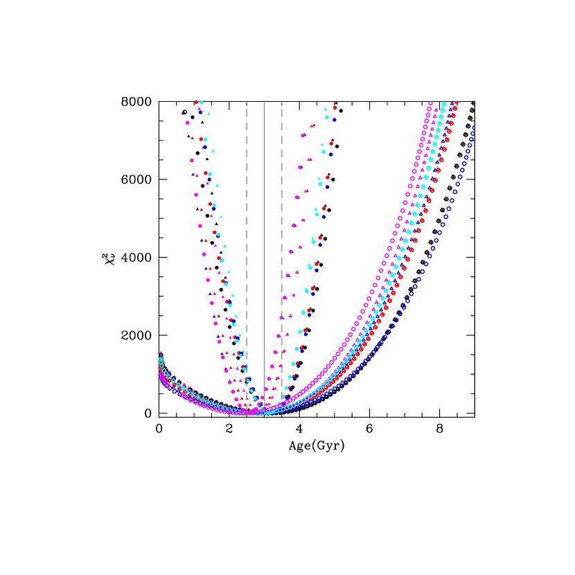
Figure 1: $\chi_{\nu}^{2}$ vs. age for the evolutionary tracks with different mixing-length parameters $\alpha_{\mathrm{MLT}}$ and different solar metallicity mixtures. Each evolutionary track has one and only one $\chi_{\nu}^{2}$-minimization model that has been listed in Table 1. Different shape symbols represent different solar mixture and different colours represent different $\alpha_{\mathrm{MLT}}$. Circles and triangles show the tracks with GS98 and AGSS09 respectively. The black, red, blue, cyan and magenta colours represent tracks with $\alpha_{\mathrm{MLT}}$ = 1.6, 1.7, 1.826, 1.9, 2.0 respectively. The solid circles and triangles show the tracks for HD176465 A, and the open circles and triangles show the tracks for HD176465 B. The solid gray vertical line indicates 3.0 Gyr, while the gray dashed lines indicate errors of 0.5 Gyr.

In order to get the best-fit model, non-asteroseismic parameters and asteroseismic parameters (mainly individual frequencies) are usually used together to obtain a total residual error $\chi^{2}$ (e.g. Lebreton 2012, Lebreton & Goupil 2014). Sometimes these parameters are used separately. Firstly, the non-asteroseismic parameters are used to narrow the range of models and then the asteroseismic parameters are used to get the best models. Owing to the high precision space-based observations, dozens of oscillation frequencies can be get for solar-like stars. Additionally, the uncertainty in the frequencies are usually much smaller than those in non-asteroseismic parameters. Some researches have been done to optimize the precision of asteroseismic inferences by matching the ratios of frequency separations or the individual frequencies (Metcalfe et al. 2014; Silva Aguirre et al. 2013). These methods improve the precision by a factor of two or more over the techniques that only use the global oscillation parameters (e.g. Lebreton & Goupil 2014; Silva Aguirre et al. 2013; Mathur et al. 2012). Recently, Wu & Li (2016, 2017) only use the observed high-precision oscillation frequencies to constrain theoretical models and determine the fundamental parameters precisely for the Sun and the solar-like oscillator KIC6225718. In this work, we calculate $\chi_{\nu}^{2}$ for all the models and then choose the $\chi_{\nu}^{2}$-minimization model on each evolutionary track as the best model for the corresponding track. At last, from all the $\chi_{\nu}^{2}$-minimization models, we select the model with minimum value of $\chi_{\nu}^{2}$ as the best-fit models for HD176465 A and B. For some models with very similar $\chi_{\nu}^{2}$, we will refer to the non-asteroseismic parameter and choose model with smaller $\chi^{2}$ as the better candidate of the star. In Table 1, we list the fundamental parameters of 10 better candidate models MA1$\sim$MA10 for HD176465 A and MB1$\sim$MB10 for HD176465 B respectively. Each candidate model with minimum value of $\chi_{\nu}^{2}$ is selected from a total of 500 evolutionary tracks with different initial combinations (M, Y_init, Z_init) and a specific mixing-length parameters $\alpha_{\mathrm{MLT}}$ and the solar metallicity mixture $(Z/X)_{\odot}$. The evolutionary tracks of these models in Table 1 are shown in Figure 1. From Figure 1, we can see that each track display regular variation of $\chi_{\nu}^{2}$ and converge to a regular shape with a unique minimum $\chi_{\nu}^{2}$. It ensure that only one model is selected as the best model for a specific evolutionary track. Additionally, Figure 1 show that the age of all the $\chi_{\nu}^{2}$-minimization models are almost in a range 3.0$\pm$0.5 Gyr that is the modelling result by White et al. (2017), in agreement with the gyrochronological value $\sim$ 3Gyr.

Table 1 show that the metallicities of models calibrated with AGSS09 are almost lower than the observed metallicity -0.3$\pm$0.06. According to the above analysis, model M8A, with minimum $\chi_{\nu}^{2}$ = 5.298 among 10 candidates MA1$\sim$MA10 in Table 1, is selected as the final best-fit model for HD176465 A. Furthermore, T_eff and [Fe/H] of M8A also match the non-asteroseismic observation within 1$\sigma$ error with $\chi^{2}_{T_{eff}}<$ 1 and $\chi^{2}_{[Fe/H]}<$ 1. As we know that, the shared formation history of binary star system result in the same age and initial chemical composition for both components of HD176465. According to Table 1, the model M8B with the combination of ($\alpha_{\mathrm{MLT}}$, $(\mathrm{Z/X})_{\odot}$) = (1.826, 0.023) (noting as $\alpha$1.826GS98), as same as M8A, is the best-fit model of HD176465 B. Although $\chi_{\nu}^{2}$ of M8B is slightly larger than that of some other models (e.g. M1B, M2B, M4B, M6B, M7B), non-asteroseismic parameters of M8B are consistent with the observations ($\chi^{2}_{T_{eff}}<$ 1 and $\chi^{2}_{[Fe/H]}<$ 1). Additionally, M8A and M8B have the same initial chemical abundance $Y_{\mathrm{init}}$ and $Z_{\mathrm{init}}$, surface metallicity [Fe/H] and age. Hence, we select the models with the combination $\alpha$1.826GS98 to deeply analyze the fundamental parameters and the interior structures of HD176465 A and B.

2.2.4 Modelling Results and Comparisons With the Work of White et al.(2017)

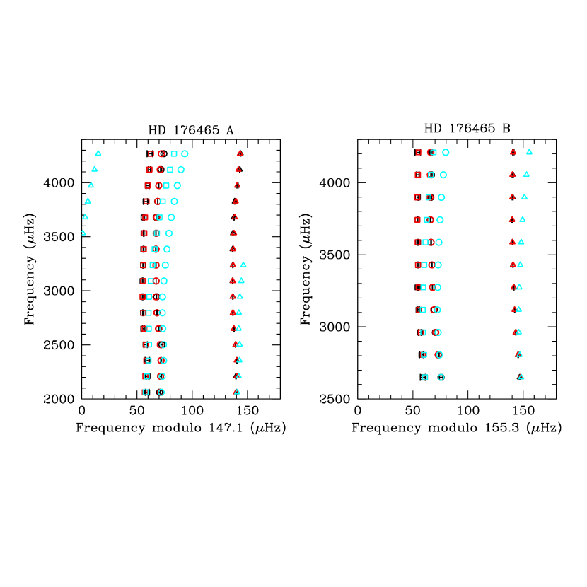
Figure 2: Échelle diagrams for HD 176465 A (left) and HD 176465 B (right). The surface corrected frequencies of best-fit models of M8A and M8B in Table 1 are indicated by the red symbols. The uncorrected frequencies of best-fit models are indicated by the cyan symbols. The black points with error bars are the observed frequencies. Different shapes of symbols represent the different modes: circles are $l$ = 0 modes, triangles are $l$ = 1 modes and squares are $l$ = 2 modes.

Figure 2 shows the echelle diagrams comparing the observed and model frequencies and thereby illustrating the quality of the match to the frequencies before and after surface-term correction using the two-term model of Ball & Gizon (2014). The large frequency separation are 147.1 $\mu$Hz and 155.3 $\mu$Hz for HD 176465 A and B respectively. They are consistent with the observations within 1$\sigma$. The large-frequency separations were calculated with surface-term corrected frequencies.

Finally, we derive the stellar parameters as the likelihood weighted mean and standard deviation from the models with minimum $\chi^{2}$ along each stellar track (see Gilliland et al. 2011 for the technique).

$$<p>=\frac{\sum\limits_{i=1}^{n}\mathcal{L}p}{\sum\limits_{i=1}^{n}\mathcal{L}},$$ (5)

$$<\sigma_{p}>=(\frac{\sum\limits_{i=1}^{n}\mathcal{L}(p-<p>)^{2}}{\sum\limits_{i=1}^{n}\mathcal{L}})^{1/2},$$ (6)

$$\mathcal{L}=(\prod\limits_{i=1}^{N}\frac{1}{\sqrt{2\pi}}\sigma_{i})\times\exp(-\chi^{2}/2),$$ (7)

where $p$ $\equiv$ [M, Y_init, Z_init, [Fe/H], age, R], $<p>$ is the likelihood weighted mean value of the fundamental parameters, $<\sigma_{p}>$ is standard deviation, $\mathcal{L}$ is the likelihood function and $\chi^{2}$ has been defined by Equation( 4). The modeling results for HD 176465 A and B are presented in Table 2 and  3. We see that, as expected, the two components of HD 176465 have the same initial composition. From the models with combination $\alpha$1.826GS98, we obtain that the current metallicities [Fe/H]${}_{\rm A}=-0.275\pm 0.04$ and [Fe/H]${}_{\rm B}=-0.285\pm 0.04$ are quite similar and consistent with the observation [Fe/H] = $-0.30\pm$ 0.06 derived by Bruntt et al. (2012). The age of the two stars $t_{\rm A}=3.087\pm 0.580$Gyr and $t_{\rm B}=3.569\pm 0.912$Gyr are, within uncertainties, the same. The results also illustrate that despite issues with surface uncertainties, asteroseismic analyses are reliable.

The detailed comparisons of fundamental parameters between our results (YREC1, YREC2) and the results of White et al. (2017) with different codes (AMP, ASTFIT, BASTA and MESA) are listed in Table 2 for HD176465 A and Table 3 for HD176465 B. According to Table 2 and  3, we can see that our results (YREC1) are more similar with the results of ASTFIT and BASTA models. These three modelling methods have almost the same input physics (including the mixing length parameter, $\alpha_{\mathrm{MLT}}$) and minimization technique. The YREC models matches individual frequencies with surface effects correction to get the best-fit model, which is the same as ASTFIT method, and the BASTA fits frequency ratios. But the mass for the primary component obtained with YREC1 is slightly larger than that of AMP, ASTFIT and BASTA models, while the YREC1 model has a lower initial helium abundance. This degeneracy between helium abundance and mass also shown in the results obtained with MESA, which is well-known in asteroseismic modelling of solar-like oscillations (Lebreton & Goupil 2014; Silva Aguirre et al. 2015). In Table 2 and  3, except ASTFIT adopted the Grevesse & Noels (1993, hereafter GN93) solar mixture, other codes used the GS98 solar mixture (Grevesse & Sauval 1998). In this work, we also get the likelihood weighted mean and standard deviation of fundamental parameters (YREC2) from models with different $\alpha_{\mathrm{MLT}}$ and AGSS09 solar mixture. From Table 2 and  3, we can see that the mass of stars with AGSS09 is slightly lower than that of other codes. The initial metallicity with AGSS09 is lowest in all the results. The current metallicities, [Fe/H]_A = -0.366 $\pm$ 0.018 and [Fe/H]_B = -0.363 $\pm$ 0.025, is poorer than the observations. For the results of White et al. (2017), four different modelling codes converge on models with mean value of mass M_A = 0.95 $\pm$ 0.02 M_⊙, M_B = 0.93 $\pm$ 0.02 M_⊙ and mean radius R_A = 0.93 $\pm$ 0.01 R_⊙, R_B = 0.89 $\pm$ 0.01 R_⊙. The ages of both components were found to be 3.0 $\pm$ 0.5 Gyr, which agree with the gyrochronological value $\sim$ 3Gyr. Our results for the mass, radius and age are consistent with those of White et al. (2017) which were determined using different codes.

3 Study of Acoustic Glitches

3.1 The Technique

The oscillatory signatures in the frequencies caused by acoustic glitches are very small. The second differences of the frequencies are usually adopted to amplify the glitch signal by suppressing the smooth variation of the frequencies to a large extent, these are defined as:

$$\delta^{2}\nu_{n,l}=\nu_{n+1,l}-2\nu_{n,l}+\nu_{n-1,l}.$$ (8)

Fitting the second differences is easier than the fit of frequencies themselves to measure the oscillatory signal (Gough 1990; Basu et al. 1994, 2004; Mazumdar & Antia 2001), however, neighbouring second-differences have correlated errors, and hence the full error-covariance matrix must be taken into account. The $\delta^{2}\nu$ are fitted to a suitable functional form that represents the glitch signatures from the base of the convective envelope and the second helium ionization zone. In this work, we use one of the functional forms suggested by Basu et al. (2004):

$$\delta^{2}\nu_{n,l}=a_{1}+a_{2}\nu+\frac{a_{3}}{\nu^{2}}\\ +\left(b_{1}+\frac{b_{2}}{\nu^{2}}\right)\sin(4\pi\nu\tau_{\rm He}+\phi_{\rm He})\\ +\left(c_{1}+\frac{c_{2}}{\nu^{2}}\right)\sin(4\pi\nu\tau_{\rm CZ}+\phi_{\rm CZ}),\\$$ (9)

where $a_{1}$, $a_{2}$, $a_{3}$, $b_{1}$, $b_{2}$, $\tau_{\rm He}$, $\phi_{\rm He}$, $c_{1}$, $c_{2}$, $\tau_{\rm CZ}$, $\phi_{\rm CZ}$ are 11 free parameters. In Equation( 9), the first three terms defines the smooth part of the second differences, the fourth term represents the oscillatory signal from the Heii ionization zone, while the last term represents the signal from the base of the convection zone. $\tau_{He}$ and $\tau_{CZ}$ are the acoustic depth of the Heii ionization zone and the base of the convection zone respectively. $b_{1}+b_{2}/{\nu^{2}}$ and $c_{1}+c_{2}/{\nu^{2}}$ are the amplitudes of acoustic glitch oscillation signature from the second helium ionization zone and the base of the convection zone respectively. In Equation( 9), the 11 unknown parameters are determined by a nonlinear least-squares fit to the second differences of the frequencies to get the parameters that give the lowest $\chi^{2}_{fit}$.

$$\chi^{2}_{fit}=\sum\limits_{i=1}^{N}[\frac{\delta^{2}\nu-\delta^{2}\nu_{fit}}{\sigma}]_{i}^{2},$$ (10)

where $\delta^{2}\nu$ is the un-fitted second differences of the observations or models, $\delta^{2}\nu_{fit}$ is the fitted second differences, $\sigma$ is the uncertainty of the $\delta^{2}\nu$ derived from individual frequencies by the error propagation.

In order to obtain the distribution of the fitted parameters, the first step of this technique is generating 1000 Monte Carlo realizations of the frequencies by adding different random perturbations to the actual frequencies with specified standard deviation equal to 1$\sigma$ uncertainty in the actual frequencies. The second step is getting 100 different initial guesses, which are selected randomly in some range of possible values, to weaken the dependence of the fitted parameters on the choice of initial guesses. The different sets of initial guesses are obtained by randomly perturbing a reasonable value for each free parameters. Because HD176465 are the solar-like oscillators with the mass similar with the Sun, firstly, the typical values of initial guesses are expected to be similar with the parameters for the Sun (e.g.$\tau_{\rm He}\sim 700s$, $\tau_{\rm CZ}\sim 2300s$). Based on the first set of initial guesses, another 99 sets of the initial parameters obtained by adding random perturbations to the first set with the standard deviation equal to 20% of the first set of parameters. Then, for each of 1000 realizations and actual frequencies, the fitting of Equation( 9) are carried out for 100 times using different initial guesses. At last, from the 100 trials, the fitting parameters with the minimum value of $\chi_{fit}^{2}$ is accepted as the best fit value for that particular realization.

For each of fitting parameters, we choose the median value from the distribution of 1001 fitting values (for 1000 realizations and actual one) as the value of the parameter. The upper 34% and lower 34% of the distribution on either side of the median is the $\pm 1\sigma$ uncertainty of the parameter.

3.2 Glitch Analysis of HD 176465

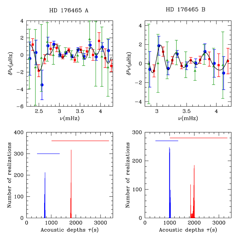
Figure 3: Upper panels: fits to the second differences of the observed frequencies for HD 176465 A (left) and B (right). The blue filled circles with error bars are the second differences for $l$ = 0 modes, the red filled squares are for $l$ = 1 modes and the green filled triangles are for $l$ = 2 modes. The solid lines show the fit to the second differences using the form given by Eq.( 9). Lower panels: the histograms of the fitted values of $\tau_{\rm He}$ (blue) and $\tau_{\rm CZ}$ (red) for different realizations. The horizontal bars at the top show the range of initial guesses for the two parameters used for fitting.

Using the technique described in § 3.1, we fit the signature of acoustic glitches in the frequencies for both components of HD 176465 to estimate the helium abundance, the acoustic depths of the Heii ionization zone $\tau_{\rm He}$ and the base of the convection envelope $\tau_{\rm CZ}$. The upper panels of Figure 3 show the fitting of the observations. The error bars of the second differences for $l=2$ mode are larger than that for $l=0$ and $l=1$ modes. This is most likely to be a result of the larger uncertainties of the $l=2$ mode frequencies. The bottom panels show the histograms of the fitted values of $\tau_{\rm He}$ (blue) and $\tau_{\rm CZ}$ (red). For HD 176465 A, $\tau_{\rm He}$ and $\tau_{\rm CZ}$ are $742_{-15}^{+10}$ s and $1806_{-12}^{+6}$ s respectively. For HD 176465 B, $\tau_{\rm He}$ and $\tau_{\rm CZ}$ are $1006_{-15}^{+28}$ s and $1979_{-125}^{+21}$ s respectively. The acoustic depth of the glitches for HD 176465 A are shallower than those of component B. This is expected because the effective temperature $T_{\rm eff}$ of component B is smaller than that of component A, and cooler stars have deeper convection zones, as well as deeper helium ionization layers (see also Verma et al. 2014b).

Besides the acoustic depth are estimated by fitting the second differences of the observations, we also calculate $\tau_{\rm He}$ and $\tau_{\rm CZ}$ from the known sound speed profile of the best-fit models (M8A and M8B in Table 1) by $\tau$ = $\int_{r}^{R}dr/c$. $r$ is the radial distance of the Heii ionization zone or the base of the convection zone. Based on the sound speed profile, we get $\tau_{\rm He}$ = 702 s and $\tau_{\rm CZ}$ = 1990 s for HD 176465 A, $\tau_{\rm He}$ = 661 s and $\tau_{\rm CZ}$ = 1899 s for HD 176465 B. From comparison of the results with two different methods, we can see that the two estimations of $\tau_{\rm CZ}$ match well for both components of HD176465. $\tau_{\rm He}$ are consistent with each other within 2.5$\sigma$ for HD176465A. But for a lower mass star HD176465 B, there is a significant difference between the two estimations of $\tau_{\rm He}$. This difference maybe result from the uncertainty in the definition of the stellar surface (Houdek & Gough 2007) and the ambiguity in the position of the Heii ionization zone (Verma et al. 2014b). As can be see from the above comparison, the robustness of fit primarily depends on the mass of star. This issue has also been discussed by Verma et al. (2017). Because HD176465 A and B are the sub-solar mass stars that are not too low in mass, the fit to the CZ signatures are robust. For low-mass stars, the depression in $\Gamma_{1}$ profile in Heii ionization zone is shallow, which result in the small amplitude of the helium signature. Especially for the sub-solar mass stars, it is difficult to fit the helium signature because of the small amplitude, unless sufficiently low radial order modes are observed. Consequently, the higher mass and more sufficient low radial order frequencies ($n$ = 13 $\sim$ 28 of $l$ = 0, 1 and $n$ = 12 $\sim$ 27 of $l$ = 2) for HD176465A than those ($n$ = 16 $\sim$ 26 of $l$ = 0, 1 and $n$ = 15 $\sim$ 25 of $l$ = 2) for HD176465 B, make the better quality of fit for primary component, which also justify the importance of the low radial order modes for improve the quality of the fitting.

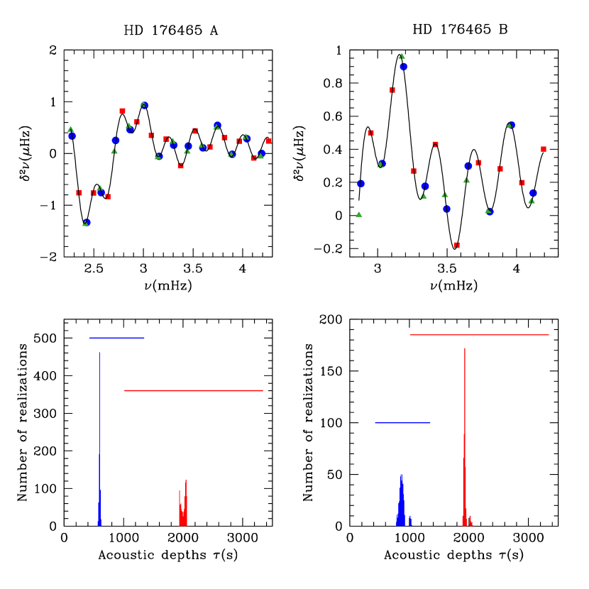
Figure 4: Fit to the second differences for the best-fit models M8A and M8B for HD 176465 A (left) and HD 176465 B (right). The symbols are same as in Figure 3

In Figure 4 we show the results for our best-fit models (M8A and M8B in Table 1), and we fit the second differences derived from the individual frequencies. The selected range of the theoretical frequencies for fit are the same as the observed frequencies (i.e. $n$ = 13 $\sim$ 28 of $l$ = 0, 1 and $n$ = 12 $\sim$ 27 of $l$ = 2 for HD176465A; $n$ = 16 $\sim$ 26 of $l$ = 0, 1 and $n$ = 15 $\sim$ 25 of $l$ = 2 for HD176465B). Comparing the fit for components A with B, we find that the fit to the CZ signature for lower-mass component B is more robust than that for component A, but that is not the case for the fit to the helium signal. The signature from the Heii ionization layers is weaker for component B which has a lower amplitude of the He signal. The distribution of the fitted parameter $\tau_{\rm He}$ have multiple peaks. We select those realizations for which the fitted acoustic depth $\tau_{\rm He}$ falls in the dominant peak to calculate the median and the error estimations. As mentioned above, the smaller number of low radial-order modes, and the larger uncertainties in the frequencies for component B make it difficult to fit the He signature. Another complicating factor is that as the mass of a star decreases, the dip in $\Gamma_{1}$ for a given helium abundance decreases too (see also Verma et al. 2014b).

In order to determine the helium abundance of HD 176465, we select all models of component A with $\chi_{\nu,{\rm A}}^{2}<50$; we refer to this set of models as Set A. For component B we select models with $\chi_{\nu,{\rm B}}^{2}<10$ (Set B). We fit the various acoustic glitch parameters for Set A using the same range of frequencies and errors as the observations for component A. We do a similar analysis for models in Set B, but using the observed mode-set of component B. We compare the observed amplitudes of the Heii ionization signature to those for the models of Set A and Set B; the models have known helium abundances and hence, can be used to calibrate the amplitude of the Heii ionization signature. Furthermore, from the models in Set A and B, we select the models with average amplitude of the Heii ionization zone signature consistent with that derived from the observed frequencies within 1$\sigma$ uncertainty, and define these models as Subset A and Subset B to estimate the helium abundance of HD176465 A and B respectively. The $\chi^{2}_{\nu}$ limits were adopted to yield a reasonable number of models to statistically analyse the helium abundance of stars; since component B has larger errors in frequencies, there are more models with lower $\chi^{2}_{\nu}$. Additionally, the large separations $\Delta\nu$ are in the range 146.83$\sim$147.17$\mu Hz$ for models in Subset A and 155.09$\sim$155.49$\mu Hz$ for models in Subset B, which are consistent with the observations ($\Delta\nu_{A}$ = 146.79 $\pm$ 0.12 $\mu Hz$, $\Delta\nu_{B}$ = 155.42 $\pm$ 0.13 $\mu Hz$) within 2$\sigma$. Hence, the choice of the thresholds for $\chi^{2}_{\nu}$ also avoid the significant deviation for the asteroseismic properties between models and observation.

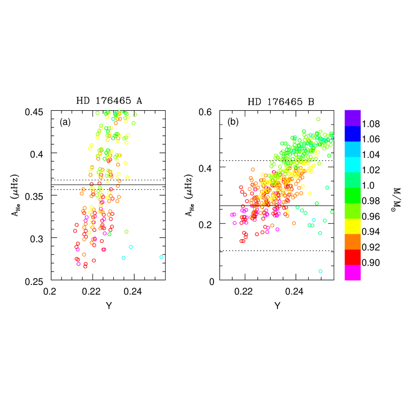
Figure 5: The average amplitude of the oscillation signature due to the Heii ionization zone of models in Sets A and B as a function of the current helium abundance in the envelope. The open circles represent the results of the models color-coded by mass. The horizontal solid line is the amplitude from observation. The dotted lines are the 1$\sigma$ uncertainty of the observed results.

Figure 5 shows the average amplitude of acoustic glitch oscillation signature from the second helium ionization zone for the observations and each selected model. In the figure, the amplitude of the Heii ionization zone signature for the observations is represented by the horizontal solid line and 1$\sigma$ uncertainty by the dotted lines. The amplitude of the Heii ionization zone signature for the observations is the median value from the distribution of 1001 average fitted amplitudes for 1000 realizations and actual observed frequencies. The upper 34% and lower 34% of the distribution on either side of the median is the $\pm$ 1$\sigma$ uncertainty of the amplitude. The open circles with different colors show the amplitude of the models with various masses. Since the amplitude is frequency dependent, the amplitudes for the observation and models are averaged over the same fitting frequency interval. From the results of the models plotted in Figure 5, we can see that, as expected, the amplitude of the Heii ionization zone signature increases with the amount of helium in the envelope. Moreover, the stellar mass and the initial helium abundance are anti-correlated (Lebreton & Goupil 2014, Silva Aguirre et al. 2015). Hence, there is some scatter due to variations in other parameters, for instance mass. Figure 5 show that, for a given helium abundance, the amplitude also increase with the mass of the star, a result of the fact that the decrease in $\Gamma_{1}$ for a given helium abundance increases with mass for our mass range. For component B, the amplitude of observation is smaller than that for component A, and the uncertainty of amplitude are much larger than component A by a factor of ten or more. Figure 3 shows that the number of the observed frequencies for component B is less than that for component A. Furthermore, the errors in the second differences are very large. These factors make it difficult to fit the Heii signature of component B. Verma et al. (2014a) have demonstrated that the precision of determination the helium abundance can be improved significantly by adding more low order mode frequencies or improving the precision of these frequencies. In order to understand this improvement, we repeat the fit of second differences of observed frequencies after removing successively the lowest three order modes of degree $l$ = 0, 1, 2 for only HD176465 A. We find that the uncertainty in the amplitude of the Heii ionization zone signature increases rapidly by a factor of ten or more. After removing the lowest order modes for HD176465 A, the uncertainty in amplitude (0.174 $\mu Hz$) is similar with that of HD176465 B (0.159 $\mu Hz$). In this case, the lowest order modes ($n$ = 16 of $l$ = 0,1 and $n$ = 15 of $l$ = 2) in fitting for HD176465 A are the same as those for HD176465 B. The amplitude of He signal is larger using the low order mode frequencies which are important for stabilizing the fitting of the helium signature.

Finally, we obtain the helium abundance for both components by calibrating the amplitude of models with observations. From the models in Subset A and B, as mentioned above, with known helium abundance, we evaluate the mean value of helium and the standard deviation of the models as the helium of HD176465 A and B, $Y_{\rm A}=0.224\pm 0.006$ and $Y_{\rm B}=0.233\pm 0.008$. The current helium abundances for HD 176465 A and B are consistent with each others within errors, the small difference could be a result of differences in settling efficiency because of the difference in masses of the two components.

3.3 Ensemble Analysis

W use the models in Sets A and B to study the variations of the acoustic glitch signature in frequencies as a function of the different stellar parameters. The large frequency separations of the models, which are calculated from the surface-term corrected frequencies, are in the range $146.7\leq\Delta\nu\leq 147.2\;\mu$Hz. Models in Set B have large separations in the range $155.1\leq\Delta\nu\leq 155.5\;\mu$Hz

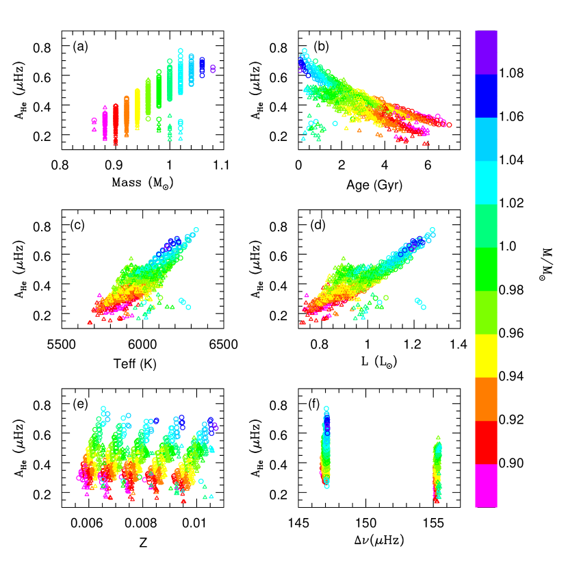
Figure 6: The variation of the average amplitude of Heii signature with mass, age, effective temperature, luminosity, metallicity and the large separation. In each panel the open circle represent models in Set A and open triangles are models in Set B. The different colors represent the different masses of the models.

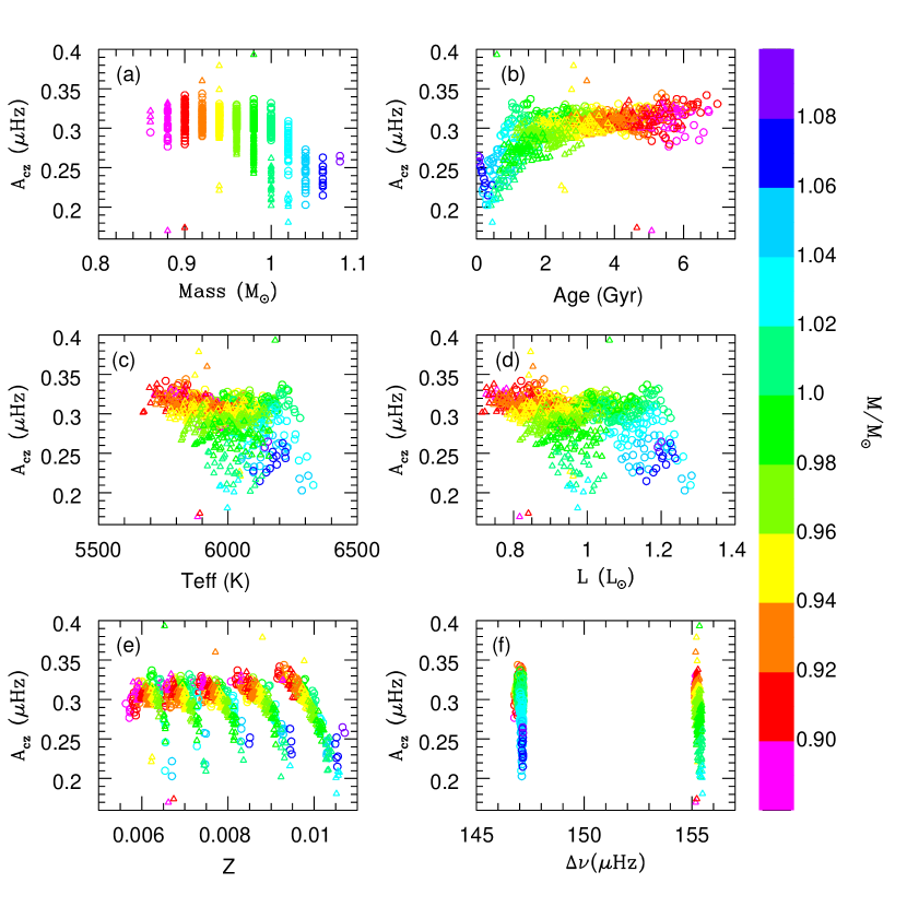
Figure 7: The same as Figure 6, but for results of the average amplitude of the base of convection zone.

Figure 6 shows the dependence of the average amplitude of Heii ionization zone signature $A_{\rm He}$ in the various stellar parameters for Set A (open circles) and Set B (open triangles). $A_{\rm He}$ increase as a function of the mass as was also seen in Figure 5. The change of $A_{\rm He}$ with effective temperature $T_{\rm eff}$ and luminosity $L$ is a reflection of the change in mass. The amplitude $A_{\rm He}$ decreases with age not only due to the lower mass with older star for a given $\Delta\nu$ but also due to the reduced helium abundance in the envelope by the helium diffusion as the star evolves. The effect of diffusion is clearly shown in panel (e). For a given initial metallicity, the lower mass star with older age has lower metallicity. For a given mass, $A_{\rm He}$ decrease with metallicity slightly. Figure 7 shows the variation of the average amplitude of the signature from the base of the convective envelope, $A_{\rm CZ}$, as a function of the different parameters. $A_{\rm CZ}$ decrease with increase in mass, effective temperature, luminosity, metallicity and the large frequency separation, while it increase with age. The variation of $A_{\rm CZ}$ is quite modest for sub-solar mass models, but for masses larger than 1.0$M_{\odot}$, $A_{\rm CZ}$ changes more rapidly.

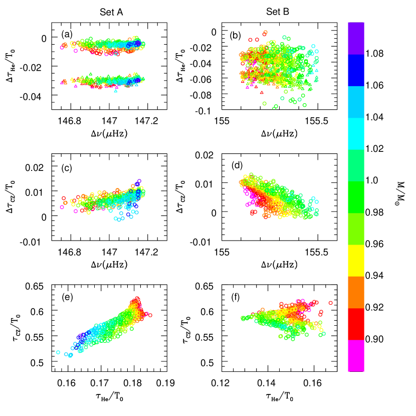
Figure 8: Panels (a) (b) show the differences of the acoustic depth of Heii ionization zone between the fitted results and obtained using the sound profile for Sets A and B respectively. The selected models are same as Figure 6. The open circles represent the scaled differences $\Delta\tau_{\rm He}/T_{0}=(\tau^{\rm fit}_{\rm He}-\tau^{c}_{He,\Gamma_{1,peak}})/T_{0}$. The open triangles represent the scale differences $\Delta\tau_{He}/T_{0}=(\tau^{fit}_{He}-\tau^{c}_{He,\Gamma_{1,dip}})/T_{0}$. Panels (c) and (d) show the scaled differences of the acoustic depth of the base of convection zone between the fitted results and obtained using the sound profile. Panels (e) and (f) show the scaled acoustic depth of the base of convection zone as a function of that of Heii ionization zone.

The study of acoustic-glitch signatures in oscillations allow us not only to estimate the helium abundance but also to detect the location of the glitches. Figure 8 shows the results for Set A (left column) and Set B (right column). In Figure 8, the top panels (a) and (b) show the scaled differences of the acoustic depth $\Delta\tau_{\rm He}/T_{0}$ between the result obtained from the fitting analysis $\tau^{\rm fit}_{He}$ and the result from calculating the sound speed profile of the model, i.e.,

$$\tau^{c}_{\rm He}=\int^{R}_{r_{\rm He}}\frac{dr}{c},$$ (11)

where $R$ is the radius of the star, $r_{He}$ is the radial distance where the Heii ionization zone is located, and $c$ is the sound speed. In panels (a) (b), open circles represent the scale differences $\Delta\tau_{\rm He}/T_{0}=(\tau^{\rm fit}_{\rm He}-\tau^{c}_{{\rm He},\Gamma_{1,peak}})/T_{0}$, where $\tau^{\rm fit}_{\rm He}$ is the value of the acoustic depth obtained by fitting the second differences. The open triangles represent the scale differences $\Delta\tau_{\rm He}/T_{0}=(\tau^{\rm fit}_{\rm He}-\tau^{c}_{{\rm He},\Gamma_{1,{\rm dip}}})/T_{0}$. $\tau^{c}_{{\rm He},\Gamma_{1,{\rm peak}}}$ is the acoustic depth corresponding to the Heii ionization zone of peak in the first adiabatic index $\Gamma_{1}$ profile between the Hei and Heii ionization. $\tau^{c}_{{\rm He},\Gamma_{1,{\rm dip}}}$ is the acoustic depth of the location of the dip in $\Gamma_{1}$. $T_{0}$ is the total acoustic radius, which are calculated from the average large separation of radial frequencies $T_{0}\approx(2\Delta\nu_{0})^{-1}$. From panels (a) and (b), we can see that the acoustic glitch of the helium ionization layer match with the acoustic depth of the peak in $\Gamma_{1}$ profile, a feature seen earlier by Broomhall et al. (2014) and Verma et al. (2014b). In Figure 8, panels (c) and (d) show the scaled difference of the acoustic depth $\Delta\tau_{\rm CZ}/T_{0}$ between the fitting analysis and the calculated result from the sound profile and the differences almost less than 0.01. Comparing the results between the He signature [panels (a) and (b)] and the CZ signature [panels (c) and (d)], we find that the quality of fit has primary dependence on mass. For the sub-solar and solar mass models, the fitting analysis to the CZ signal was robust, while the fit to the Heii ionization signal was not good especially for the models with mass less than 0.9 $M_{\odot}$ due to the smaller amplitude of the peak in $\Gamma_{1}$ profile between the Hei and Heii ionization. The lowermost panels (e) and (f) of Figure 8 show the clear correlation between the scale acoustic depth of the base of convection envelope and the second helium ionization zone especially for Set A, but not for models with mass less than 0.9 $M_{\odot}$ again due to the difficulty of fitting for lower mass star. The positive correction between $\tau_{\rm CZ}/T_{0}$ and $\tau_{\rm He}/T_{0}$ show that the cooler star with lower mass have the deeper convection envelope and the second helium ionization zone.

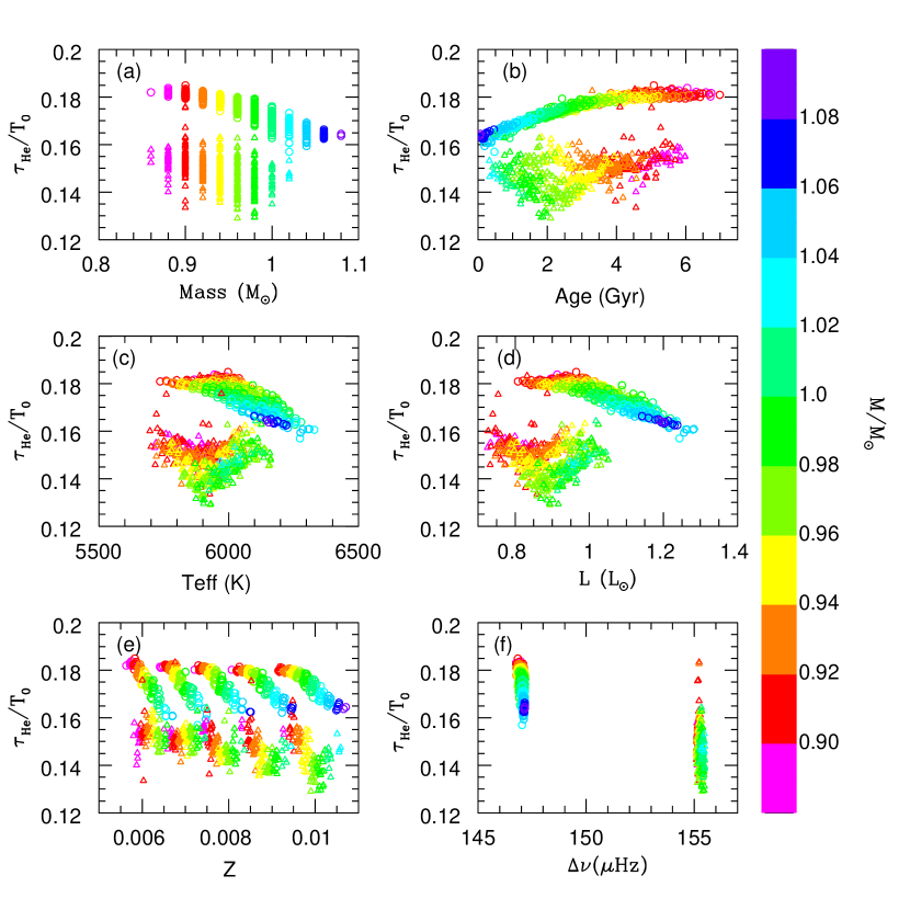
Figure 9: The variation of the scaled acoustic depth of Heii ionization zone with mass, age, effective temperature, luminosity, metallicity and the large separation respectively. The selected models are same as Figure 6. In each panel of figure, the open circle represent the Set A which calibrated by the observations of component A. The open triangle represent the Set B which calibrated by the observations of component B. Different colors show the different masses of stellar models.

Figure 9 shows the scaled acoustic depth of Heii ionization zone signature $\tau_{\rm He}/T_{0}$ from fitting analysis as a function of mass, age, $T_{\rm eff}$, $L$, $Z$ and $\Delta\nu$. $\tau_{\rm He}/T_{0}$ decrease with the increased mass, $T_{\rm eff}$, $L$, $Z$ and $\Delta\nu$, while it increase as the star evolve. This is again show that the hotter star with larger mass has the shallower helium ionization zone. Comparing the results for Set A (open circles) and Set B (open triangles), the larger dispersion of the result for Set B show that more sufficient and precise low radial mode observed frequencies of component B are needed to improve the quality of the fits to Set B.

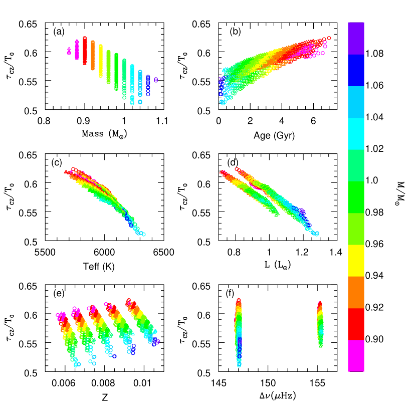
Figure 10: The variation of the scaled acoustic depth of the base of convection zone with mass, age, effective temperature, luminosity, metallicity and the large separation respectively. The selected models and symbols are same as Figure 6.

Figure 10 shows that there are clear dependence of $\tau_{\rm CZ}/T_{0}$ on various stellar parameters for both Sets A and B. Comparing the results in Figure 10 with Figure 9, we find that the fit to the base of the convective envelope is more robust than the fit to the Heii ionization signal for sub-solar mass stars. In each panel of Figure 10, the vertical distribution of $\tau_{\rm CZ}/T_{0}$ show that the dependence of $\tau_{\rm CZ}/T_{0}$ on mass is significantly greater than on other parameters. For a given mass, poorer metallicity models have lower opacity, resulting in a shallower convective envelope.

4 Conclusions

We have used observed mode frequencies and spectroscopic parameters to derive the stellar parameters for binary system HD 176465. The masses and radii of both components are consistent with the earlier estimates of White et al. (2017) using different codes. Although we fit the observations of HD 176465 A and B individually, we find that both models have the same initial abundances ($Y_{\mathrm{init},{\rm A}}=0253\pm 0.006$ and $Y_{\mathrm{init},{\rm B}}=0.254\pm 0.008$; $Z_{\mathrm{init}}=0.010\pm 0.001$ for both components). The current metallicity of the two components are also very similar ([Fe/H]${}_{\rm A}=-0.275\pm 0.04$ and [Fe/H]${}_{\rm B}=-0.285\pm 0.04$); note these are lower than the initial metallicity because of the gravitational settling of element diffusion. Although the ages of two stars of HD 176465 are not a priori constrained to be the same, the age of both components ($t_{\rm A}=3.087\pm 0.580$ Gyr and $t_{\rm B}=3.569\pm 0.912$ Gyr) are the same within errors. This show that both components of HD 176465 are the young sub-solar mass stars, with masses of $0.975\pm 0.040$ M_⊙ and $0.932\pm 0.022$ M_⊙.

Additionally, we used the glitch signal in the frequencies caused by the depression in $\Gamma_{1}$ at the second helium ionization zone to determine the current envelope helium abundance of the stars. We used the technique of fitting the second differences in frequencies to the function proposed by Basu et al. (2004). However, the exact form of the amplitudes of glitch signatures or the different techniques to remove the smooth term in the frequencies does not affect the results significantly (Basu et al. 2004; Verma et al. 2014a). We estimate the current helium abundance ($Y_{\rm A}=0.224\pm 0.006$ and $Y_{\rm B}=0.233\pm 0.008$) for both components, which are lower than the initial helium abundance because of the effect of element diffusion. The small difference of helium depletion is consistent with what is expected from the small difference in mass between the two components of the binary.

We selected two sets of models whose asteroseismic properties are very close to those of the two components of HD 176465 to study the properties of the acoustic glitch signatures arising from the second helium ionization layer and the base of the convective envelope. The amplitude of Heii signature $A_{\rm He}$ is predominantly a function of the helium abundance. $A_{\rm He}$ also increase with mass, effective temperature, luminosity and decrease as the star evolves. The variation of the amplitude of the base of convection zone ($A_{\rm CZ}$) is quite modest for sub-solar mass models. Furthermore, we determined the location of the He and CZ signatures and confirmed that acoustic depth of the helium ionization layer matches the acoustic depth of the peak in $\Gamma_{1}$ profile between the Hei and Heii ionization zones. The fit to the CZ signature are robust for low-mass star with mass less than 1.0 $M_{\odot}$. The acoustic depth of convection zone $\tau_{\rm CZ}$ is sensitive to the metallicity because of the poorer metallicity have lower opacity, hence shallower convective envelopes. The dependence of $\tau_{\rm CZ}$ on the metallicity can be used to constrain the metallicity. The fit of the He signature are weak for the models with mass less than 0.9 $M_{\odot}$ because of the smaller amplitude of the peak in $\Gamma_{1}$. The acoustic depth between $\tau_{\rm CZ}$ and $\tau_{\rm He}$ present a clear positive correlation, which show that the deeper convection envelope and the deeper second helium ionization zones for the cooler low mass star. The robust fit of CZ signature for lower mass star and the positive correlation between $\tau_{\rm CZ}$ and $\tau_{\rm He}$ can help us in estimating $\tau_{\rm He}$ for stars with masses less than 0.9 $M_{\odot}$. Besides the effect of mass, the more sufficient and precise low radial mode observed frequencies can help to improve the quality of the fit.

Table 1: Properties of the better candidate models for HD 176465 A and B

star	$\alpha_{\mathrm{MLT}}$	M	Age	Yint	Zint	[Fe/H]	R	Teff	$\Delta\nu$	$\nu_{max}$	$\chi^{2}_{T_{eff}}$	$\chi^{2}_{[Fe/H]}$	$\chi^{2}_{\nu}$	$\chi^{2}$	$a_{\mathrm{cubic}}$	$a_{\mathrm{inv}}$
HD176465		(M⊙)	(Gyr)				(R${}_{\odot})$		($\mu Hz$)	($\mu Hz$)
(Z/X)⊙=0.019(AGSS09)
M1A	1.6	0.94	3.245	0.254	0.0084	-0.3612	0.922	5860	147.08	3389	0.114	1.041	6.704	7.859	3.245	-11.203
M1B	1.6	0.90	3.108	0.258	0.0067	-0.4594	0.876	5871	155.26	3597	2.127	7.054	0.948	10.129	3.108	-11.167
M2A	1.7	0.96	2.761	0.254	0.0084	-0.3556	0.929	5957	147.07	3388	1.984	0.858	6.272	9.114	2.761	-11.205
M2B	1.7	0.92	2.798	0.254	0.0067	-0.4548	0.883	5945	155.27	3598	5.194	6.659	0.989	12.842	2.798	-9.176
M3A	1.826	0.98	2.596	0.250	0.0085	-0.3529	0.935	6037	147.05	3386	5.311	0.778	6.499	12.588	2.596	-9.451
M3B	1.826	0.94	2.660	0.258	0.0084	-0.3486	0.889	5954	155.28	3619	5.655	0.656	1.040	7.351	2.660	-10.323
M4A	1.9	0.96	3.170	0.258	0.0084	-0.3618	0.929	6064	147.04	3358	6.745	1.060	6.531	14.336	3.170	-10.552
M4B	1.9	0.94	2.760	0.250	0.0068	-0.4538	0.889	6053	155.25	3594	12.083	6.567	0.965	19.615	2.760	-9.678
M5A	2.0	0.98	2.869	0.254	0.0084	-0.3574	0.935	6127	147.02	3362	10.913	0.915	6.165	17.993	2.869	-9.138
M5B	2.0	0.94	2.827	0.254	0.0067	-0.4556	0.888	6111	155.23	3578	17.016	6.729	1.068	24.813	2.827	-9.336
(Z/X)⊙=0.023(GS98)
M6A	1.6	0.96	3.220	0.250	0.0107	-0.2515	0.930	5756	147.14	3434	0.671	0.652	5.797	7.120	3.220	-10.011
M6B	1.6	0.90	3.114	0.258	0.0067	-0.4563	0.876	5867	155.25	3599	2.006	6.783	0.969	9.758	3.114	-11.869
M7A	1.7	0.96	3.181	0.258	0.0106	-0.2531	0.930	5854	147.11	3410	0.069	0.610	5.439	6.118	3.181	-10.677
M7B	1.7	0.92	2.801	0.254	0.0068	-0.4517	0.882	5941	155.27	3601	5.009	6.394	0.953	12.356	2.801	-10.076
M8A	1.826	0.98	3.227	0.250	0.0107	-0.2521	0.936	5913	147.12	3415	0.853	0.638	5.298	6.789	3.227	-10.578
M8B	1.826	0.96	2.802	0.250	0.0107	-0.2416	0.896	5827	155.34	3676	0.935	0.947	0.994	2.876	2.802	-10.251
M9A	1.9	0.98	3.139	0.250	0.0096	-0.3039	0.936	6007	147.07	3389	3.893	0.004	5.589	9.486	3.139	-9.083
M9B	1.9	0.94	2.766	0.250	0.0068	-0.4507	0.888	6049	155.25	3598	11.816	6.307	1.023	19.146	2.766	-10.593
M10A	2.0	1.00	2.579	0.258	0.0106	-0.2468	0.943	6079	147.07	3390	7.704	0.787	5.527	14.018	2.579	-8.129
M10B	2.0	0.96	2.402	0.258	0.0085	-0.3428	0.896	6068	155.28	3607	13.321	0.508	1.081	14.910	2.402	-8.206

Table 2: Comparison of our results (YREC1 and YREC2) with those obtained using other codes (AMP, ASTFIT, BASTA and MESA) by white et al. (2017) for HD 176465 A.

Property	AMP	ASTFIT	BASTA	MESA1	MESA2	YREC1	YREC2
M/M⊙	0.930$\pm$0.04	0.952$\pm$0.015	0.960${}^{+0.010}_{-0.011}$	0.95$\pm$0.03	0.99$\pm$0.02	0.975$\pm$0.016	0.944$\pm$0.018
Yinit	0.258$\pm$0.024	0.262$\pm$0.003	0.265$\pm$0.002	0.25$\pm$0.02	0.23$\pm$0.02	0.253$\pm$0.006	0.256$\pm$0.005
Zinit	0.0085$\pm$0.0010	0.0103$\pm$0.0010	0.011$\pm$0.004	0.0102$\pm$0.0009	0.0094$\pm$0.0009	0.0102$\pm$0.0008	0.0083$\pm$0.0003
Age(Gyr)	3.0$\pm$0.4	3.2$\pm$0.5	2.8$\pm$0.3	3.2$\pm$0.2	3.01$\pm$0.12	3.087$\pm$0.580	3.146$\pm$0.535
R/R⊙	0.918$\pm$0.015	0.927$\pm$0.005	0.928${}^{+0.006}_{-0.003}$	0.926$\pm$0.011	0.939$\pm$0.006	0.934$\pm$0.005	0.923$\pm$0.006
$\alpha_{\mathrm{MLT}}$	1.90$\pm$0.18	1.80	1.791	1.57$\pm$0.11	1.79	1.826	1.81$\pm$0.14
(Z/X)⊙	0.023(GS98)	0.0245(GN93)	0.023(GS98)	0.023(GS98)	0.023(GS98)	0.023(GS98)	0.018(AGSS09)

Table 3: Comparison of our results (YREC1 and YREC2) with those obtained using other codes (AMP, ASTFIT, BASTA and MESA) by white et al. (2017) for HD 176465 B.

Property	AMP	ASTFIT	BASTA	MESA1	MESA2	YREC1	YREC2
M/M⊙	0.930$\pm$0.02	0.92$\pm$0.02	0.929${}^{+0.010}_{-0.011}$	1.02$\pm$0.07	0.97$\pm$0.04	0.932$\pm$0.022	0.914$\pm$0.021
Yinit	0.246$\pm$0.013	0.262$\pm$0.003	0.265$\pm$0.002	0.21$\pm$0.04	0.24$\pm$0.04	0.255$\pm$0.008	0.257$\pm$0.006
Zinit	0.0085$\pm$0.0007	0.0096$\pm$0.0011	0.011$\pm$0.004	0.0124$\pm$0.0015	0.0122$\pm$0.0011	0.0099$\pm$0.0008	0.0083$\pm$0.0004
Age(Gyr)	2.9$\pm$0.5	3.4$\pm$0.9	3.2$\pm$0.4	2.9$\pm$0.4	3.18$\pm$0.31	3.569$\pm$0.912	3.226$\pm$0.944
R/R⊙	0.885$\pm$0.006	0.883$\pm$0.007	0.886${}^{+0.003}_{-0.006}$	0.919$\pm$0.021	0.899$\pm$0.013	0.887$\pm$0.007	0.883$\pm$0.007
$\alpha_{\mathrm{MLT}}$	1.94$\pm$0.12	1.80	1.791	2.05$\pm$0.28	1.79	1.826	1.81$\pm$0.14
(Z/X)⊙	0.023(GS98)	0.0245(GN93)	0.023(GS98)	0.023(GS98)	0.023(GS98)	0.023(GS98)	0.018(AGSS09)

References

- Angulo et al. (1999) Angulo, C., Arnould, M., Rayet, M., et al. 1999, Nucl. Phys. A., 656, 3
- Asplund et al. (2009) Asplund, M. Grevesse, N., Sauval, A. & Scott, P. 2009, ARA&A, 47, 481
- Ball & Gizon (2014) Ball, W. H. & Gizon, L. 2014, A&A, 568, A123
- Basu et al. (1994) Basu, S., Antia, H. M., & Narasimha, D. 1994, MNRAS, 267, 209
- Basu & Antia (1995) Basu, S. & Antia H. M. 1995, MNRAS, 276, 1402
- Basu et al. (2004) Basu, S., Mazumdar, A., Antia, H. W. & Demarque, P. 2004, MNRAS, 350,277
- Basu & Antia (2008) Basu, S. & Antia, H. M. 2008, PhR, 457, 217
- Basu (2016) Basu, S. 2016, LRSP, 13, 2
- Broomhall et al. (2014) Broomhall, A. -M., Miglio, A., Montalbán, J., et al. 2014, MNRAS, 440, 1828
- Bruntt et al. (2012) Bruntt, H., Basu, S., Smalley, B., et al. 2012, MNRAS, 423, 122
- Caffau et al. (2010) Caffau, E., Ludwig, H.-G., Bonifacio, P., Faraggiana, R. et al. 2010, A&A, 514, A92
- Christensen-Dalsgaard et al. (2011) Christensen-Dalsgaard, J., Monteiro, M. J. P. F. G., Rempel, M., & Thompson, M. J. 2011, MNRAS, 414, 1158
- Demarque et al. (2008) Demarque, P., Guenther, D. B., Li, L. H., Mazumdar, A. & Straka, C. W. 2008, Ap&SS, 316, 31
- Ferguson et al. (2005) Ferguson, J. W., Alexander, D. R., Allard, F., et al. 2005, ApJ, 623, 585
- García et al. (2011) García, R. A., Hekker, S., Stello, D., et al. 2011, MNRAS, 414, L6
- Gilliland et al. (2011) Gilliland, R.L, McCullough, P.R., Nelan, E.P., et al. 2011, ApJ, 726, 2
- Gough (1990) Gough, D. O. 1990, in Progress of Seismology of the Sun and Stars, ed. Y. Osaki & H. Shibahashi (Lecture Notes in Physics, Vol. 367; Berlin: Springer), 283
- Gough & Thompson (1988) Gough, D. O., & Thompson, M. J. 1988, in IAU Symp. 123, Advances in Helio- and Asteroseismology, ed. J. Christensen-Dalsgaard & S. Frandsen (Dordrecht: Reidel), 155
- Grevesse & Noels (1993) Grevesse, N. & Noels, A. 1993, in Origin and Evolution of the Elements, ed. S. Kubono & T. Kajino, 15
- Grevesse & Sauval (1998) Grevesse, N. & Sauval, A. J. 1998, Space Sci. Rev., 85, 161
- Guenther (1994) Guenther, D. B. 1994, ApJ, 422, 400
- Houdek (2004) Houdek, G. 2004, in AIPConf. Proc. 731, Equation-of-state and Phase-transition Issues in Models of Ordinary Astrophysical Matter, ed. V. Celebonovic, W. D appen, & D. O. Gough (Melville, NY: AIP), 193
- Houdek & Gough (2006) Houdek, G., & Gough, D. O. 2006, in Proc. SOHO18/GONG 2006/HELAS I: Beyond the Spherical Sun, ed. M. Thompson & K. Fletcher (ESA SP-624; Noordwijk: ESA), 88
- Houdek & Gough (2007) Houdek, G., & Gough, D. O. 2007, MNRAS, 375, 861
- Howe et al. (2017) Howe, R., Basu, S., Davies, G. R., Ball, W. H. et al. 2017, MNRAS, 464, 4777
- Iglesias & Rogers (1996) Iglesias, C. A. & Rogers, F. J. 1996, ApJ, 464, 943
- Jenkins et al. (2010) Jenkins, J. M., Caldwell, D. A., Chandrasekaran, H. et al. 2010, ApJ, 713, L87
- Lebreton (2012) Lebreton, Y. 2012, in ASP Conf. Ser. 462, Progress in Solar/Stellar Physics with Helio- and Asteroseismology, ed. H. Shibahashi, M. Takata, & A. E. Lynas-Gray (San Francisco, CA: ASP), 469
- Lebreton & Goupil (2014) Lebreton, Y. & Goupil, M. J. 2014, A&A, 569, A21
- Lodders et al. (2009) Lodders, K., Palme, H. & Gail, H-P. 2009, LanB, 4B, 44
- lund et al. (2017) Lund, M. N., Silva Aguirre, V., Davies, G. R., et al. 2017, ApJ, 835, 172
- Mathur et al. (2012) Mathur, S., Metcalfe, T. S., Woitaszek, M. et al. 2012, ApJ, 749, 152
- Mazumdar & Antia (2001) Mazumdar, A. & Antia, H. M. 2001, A&A, 377, 192
- Mazumdar et al. (2012) Mazumdar, A., Michel, E., Antia, H. M. & Deheuvels, S. 2012, A&A, 540, A31
- Mazumdar et al. (2014) Mazumdar, A., Monteiro, M. J. P. F. G., Ballot, J., Antia, H. M., Basu, S., et al. 2014, ApJ, 782, 18
- Metcalfe et al. (2014) Metcalfe, T. S., Creevey, O. L., Dogan, G. et al. 2014, ApJS, 214,27
- Miglio et al. (2010) Miglio, A., Montalbn, J., Carrier, F., et al. 2010, A&A, 520, L6
- Monteiro et al. (1994) Monteiro, M. J. P. F. G., Christensen-Dalsgaard, J. & Thompson, M. J. 1994, A&A, 283, 247
- Monteiro et al. (2000) Monteiro, M. J. P. F. G., Christensen-Dalsgaard, J. & Thompson, M. J. 2000, MNRAS, 316, 165
- Rogers & Nayfovov (2002) Rogers, F. J. & Nayfonov, A. 2002, ApJ, 576, 1064
- Roxburgh & Vorontsov (1994) Roxburgh, I. W. & Vorontsov, S. V. 1994, MNRAS, 268, 880
- Roxburgh & Vorontsov (2003) Roxburgh, I. W. & Vorontsov, S. V. 2003, A&A, 411, 215
- Schmitt & Basu (2015) Schmitt, J. R. & Basu, S. 2015, ApJ, 808, 123
- Serenelli & Basu (2010) Serenelli, A., Basu, S. 2010, ApJ, 719, 865
- Silva Aguirre et al. (2013) Silva Aguirre, V., Basu, S., Brandao, I. M. et al. 2013, ApJ, 769, 141
- Silva Aguirre et al. (2015) Silva Aguirre, V., Davies, G. R., Basu, S. et al. 2015, MNRAS, 452, 2127
- Steigman (2010) Steigman, G. 2010, J.Cosmology Astropart. Phys., 04, 029
- Thoul et al. (1994) Thoul, A. A., Bahcall, J. N. & Loeb, A. 1994, ApJ, 421, 828
- Verma et al. (2014a) Verma, K., Faria, J. P., Antia, H. M., Basu, S., et al. 2014a, ApJ, 790, 138
- Verma et al. (2014b) Verma, K., Antia, H. M., Basu, S. & Mazumdar, A. 2014b, ApJ, 794, 114
- Verma et al. (2017) Verma, K., Raodeo, K., Antia, H. M., Mazumdar, A., et al. 2017, ApJ, 837, 47
- Vorontsov (1988) Vorontsov, S. V. 1988, in IAU Symp, 123, Advances in Helio- and Asteroseismology, ed. J. Christensen-Dalsgaard & S. Frandsen (Dordrecht: Reidel), 151
- White et al. (2017) White, T. R., Benomar, O., Silva Aguirre, V., Ball, W. H., et al. 2017, A&A, 601, 82
- Wu & Li (2016) Wu, T. & Li, Y. 2016, ApJ, 818L, 13
- Wu & Li (2017) Wu, T. & Li, Y. 2017, ApJ, 846, 41
- Yang (2016) Yang, W. M. 2016, ApJ, 821, 108