Phase amplification in optical interferometry with weak measurement

Abstract

Improving the phase resolution of interferometry is crucial for high-precision measurements of various physical quantities. Systematic phase errors dominate the phase uncertainties in most realistic optical interferometers. Here we propose and experimentally demonstrate a weak measurement scheme to considerably suppress the phase uncertainties by the direct amplification of phase shift in optical interferometry. Given an initial ultra-small phase shift between orthogonal polarization states, we observe the phase amplification effect with a factor of 388. Our weak measurement scheme provides a practical approach to significantly improve the interferometric phase resolution, which is favorable for precision measurement applications.

I introduction

Interferometry is one of the most important metrology tools by transforming the measurements of various physical quantities into phase measurements. The precision of measurement highly depends on the phase resolution of interferometry. The phase resolution is limited by the uncertainty contributions of two parts, i.e., statistical phase errors and systematic phase errors. For a given sample size $N$, the statistical errors are described as the standard quantum limit, i.e., $\frac{1}{\sqrt{N}}$. Quantum-enhanced measurements as resource-efficient methods are often used to beat the standard quantum limit Giovannetti04 ; Giovannetti11 ; Boto00 ; Holland93 ; Caves81 . For instance, given a $n$-qubit entangled $N00N$ state $\frac{1}{\sqrt{2}}(|0\rangle^{\otimes{n}}+|1\rangle^{\otimes{n}})$, due to its characteristic of phase super-sensitivity Boto00 , the statistical errors can be decreased down to $\frac{1}{\sqrt{nN}}$.

In realistic optical interferometers, the systematic phase errors due to device imperfections often dominate the phase uncertainty, which cannot be reduced by averaging. For instance, the phase uncertainty of measuring the phase shift between two orthogonal polarization components is mainly attributed to alignment errors of polarization devices in interferometers. In such case, the phase uncertainty is bounded by $\frac{1}{\sqrt{e}}$, which $e$ is the polarization extinction ratio (PER) of polarization devices, since the minimal probability of projection measurement is at the order of $\frac{1}{e}$. Therefore, to improve the phase resolution of optical interferometers reducing the contribution of the intrinsic phase errors is crucial.

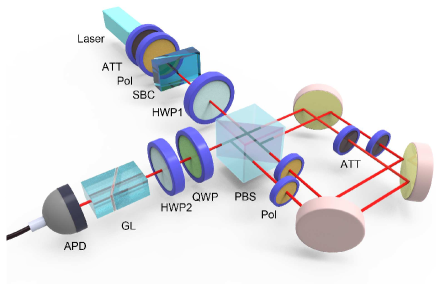
Figure 1: Experimental setup. Focused laser pulses with a center wavelength of 785 nm pass through a set of attenuators to prepare the incident photon source, and the attenuated intensity of the source is less than one million photons per second. A polarizer is placed after the attenuator to prepare the initial polarization state of $\frac{1}{\sqrt{2}}(|H\rangle+|V\rangle)$. An initial tiny phase is generated by the SBC between $|H\rangle$ and $|V\rangle$. HWP1 is used to implement the unitary rotation $U\left(\alpha\right)$. Then the beam passes through a Sagnac-like interferometer with two tunable attenuators and two polarizers in two different paths. The angles of the polarizers are placed at $|H\rangle$ and $|V\rangle$ for the transmitted and reflected photons, respectively, in order to increase the polarization visibility. The tunable attenuators are used to balance the intensity in two paths. The two arms of the interferometer are separate with only 4 mm so that the stability of interferometer can be effectively guaranteed. A QWP set at the angle of $\pi/4$ and HWP2 are used to project polarization states to $(|H\rangle+e^{i\beta}|V\rangle)/\sqrt{2}$, in which the modulated phase delay $\beta$ is implemented by tuning the angle of HWP2. ATT: attenuator; Pol: polarizer; SBC: Soleil-Babinet Compensator; HWP: half-wave plate; QWP: quarter-wave plate; PBS: polarizing beam splitter; GL: Glan-Laser Calcite Polarizer; APD: avalanche photodiode.

We first analyze the interferometric phase uncertainty using single-qubit states. Considering the typical configuration of a realistic optical interferometer to measure a small initial phase, the detection probability at one output port of the interferometer can be calculated as

$$p=\frac{1}{2}(1+\cos(\phi+\varphi)),$$ (1)

where $\phi$ is the phase to be measured, and $\varphi$ is the systematic phase error due to device imperfections. Generally, $\varphi$ can be described as a zero-mean random phase error following a Gaussian distribution $e^{-\frac{\varphi^{2}}{2\rho^{2}}}$ with a standard deviation of $\rho$. Given a sample size of $N$, the total phase uncertainty is (see Eq. (A10) in Appendix A)

$$\Delta\phi=\sqrt{\rho^{2}+\frac{1}{N}},$$ (2)

where the systematic phase errors and the statistical phase errors are related with the terms of $\rho$ and $\frac{1}{\sqrt{N}}$, respectively, and $\rho$ is often much larger than $\frac{1}{\sqrt{N}}$ for realistic optical interferometers. When using $N00N$ states instead of single-qubit states, the detection probability ($p^{(N)}$) is then changed to

$$p^{(N)}=\frac{1}{2}(1+\cos(n\phi+\varphi)).$$ (3)

The total phase uncertainty in this scenario is $\sqrt{\frac{\rho^{2}}{n^{2}}+\frac{1}{nN}}$ (see Eq. (A13) in Appendix A). However, preparing multi-qubit entangled states with large $n$ is proven notoriously challenging. The largest number of entangled photons created so far is 10 Wang16 ; Chen17 in a probabilistic way, limiting the practical advantage of using $N00N$ states to improve the phase resolution.

Weak measurement is a new quantum-mechanical approach to further suppress the phase uncertainty. The concept of weak measurement was discovered in 1980s Aharonov88 . So far diverse weak measurement schemes have been proposed for the applications of precise measurements due to the advantages of amplification effects Aharonov90 ; Feizpour11 ; Zilberberg11 ; Wu12 ; Strubi13 ; Pang14 , which can be used to effectively overcome the device imperfections. Experiments using weak measurement schemes have demonstrated to perform the precise measurements of certain quantities such as ultra-small transverse split Hosten08 , beam deflection Dixon09 , light chirality Gorodetski12 and angular rotation Magana14 . Specifically, Brunner and Simon Brunner10 proposed a scheme to convert the quantity of time delay to frequency shift using imaginary weak-value amplification. Based on this scheme, Xu et al. Xu13 demonstrated to measure a time delay at the order of attosecond, corresponding to a phase resolution of a few mrad, using a commercial light-emitting diode and a spectrometer, and Salazar-Serrano et al. SS14 implemented a sub-pulse-width time delay measurement as small as 22 femtoseconds using a femtosecond fiber laser. Recently, Qiu et al. Xiaodong17 reported an approach to convert phase estimation to intensity measurement with imaginary weak-value amplification, showing a phase resolution $\sim$ $1$ mrad.

II scheme

In this Letter, we propose and experimentally demonstrate a new weak measurement scheme, in which the amplification of phase shifts in an interferometer can be directly implemented. The experimental results clearly show that the phase resolution of interferometer can be improved with 2$\sim$3 orders of magnitudes besides the conventional techniques for phase stabilization.

In our weak measurement scheme, it is assumed that the input qubit state is $\frac{1}{\sqrt{2}}(|H\rangle+e^{i\phi}|V\rangle)$, where $|H\rangle\left(|V\rangle\right)$ represents the horizontal (vertical) polarization state of photons, and $\phi$ is the initial phase shift to be measured. After passing a half-wave plate with a unitary rotation

$$U\left(\alpha\right)=\left(\begin{array}[]{cc}\cos\alpha&\sin\alpha\\ -\sin\alpha&\cos\alpha\end{array}\right),$$ (6)

where $\alpha=\pi/4-\varepsilon$ and $\varepsilon\ll 1,$ the input state is transformed to $\left(\cos\alpha+e^{i\phi}\sin\alpha\right)|H\rangle+\left(-\sin\alpha+e^{i\phi}\cos\alpha\right)|V\rangle$. Then the final phase shift between $|H\rangle$ and $|V\rangle$ components is

$$\phi^{\prime}=ang\left(\sin 2\varepsilon\cos\phi+i\sin\phi\right),$$ (7)

where the function $ang$ represents the phase angle of a complex value. In the case of $\phi\ll 1$ and $\phi/\varepsilon\ll 1$, the transformed polarization state is approximately equivalent to $(|H\rangle+\varepsilon e^{\frac{i\phi}{2\varepsilon}}|V\rangle)/\sqrt{1+\varepsilon^{2}}$, from which one can clearly find out that the relative phase shift is amplified. After passing through a polarizing beam splitter in the interferometer, this state can be written as $(|H\rangle|0\rangle+\varepsilon e^{\frac{i\phi}{2\varepsilon}}|V\rangle|1\rangle)/\sqrt{1+\varepsilon^{2}}$, where $\left\{|0\rangle,|1\rangle\right\}$ represents the path degree of freedom in the interferometer.

Further, in order to suppress the phase uncertainty induced by the systematic phase errors and thus improve the phase resolution of interferometer with such transformed polarization state, it is still required to attenuate the intensity of $|H\rangle$ component down to the same level as $|V\rangle$ component. After the attenuation, the final qubit state is changed to $\frac{1}{\sqrt{2}}(|H\rangle+e^{\frac{i\phi}{2\varepsilon}}|V\rangle),$ with a successful probability of $\thicksim 2\varepsilon^{2}$. We note that attenuating the intensity of $|H\rangle$ component is equivalent to project the path state to $|f\rangle=\left(\varepsilon|0\rangle+|1\rangle\right)/\sqrt{1+\varepsilon^{2}}.$ Due to the effect of phase shift amplification, the phase uncertainty of the interferometer is thus improved to (see Eq. (A16) in Appendix A)

$$\Delta\phi=2\sqrt{\varepsilon^{2}\rho^{2}+\frac{1}{2N}}.$$ (8)

Although the contribution of statistical phase errors is multiplied by $\sqrt{2}$, the contribution of systematic phase errors is drastically suppressed by a factor of $2\varepsilon$. Therefore, with the help of weak measurement, the phase resolution of interferometer can be improved by a factor of $\frac{1}{2\varepsilon}$, when $\rho\gg\frac{1}{\sqrt{N}}$.

From the perspective of weak measurement, the path degree of freedom can be treated as a system, and the polarization degree of freedom can be treated as a qubit meter Wu09 . The coupling of the system and the meter is described by

$$\frac{1}{\sqrt{2(1+\varepsilon^{2})}}e^{\frac{1}{4}i\pi\sigma_{y}\otimes\left(\sigma_{z}-I\right)}\left(|L\rangle+|R\rangle\right)\otimes\left(|H\rangle+\varepsilon e^{i\phi^{\prime}}|V\rangle\right),$$ (9)

where $|L\rangle$ and $|R\rangle$ are the eigenstates of Pauli matrix $\sigma_{y}$, i.e., $\frac{1}{\sqrt{2}}\left(|0\rangle\pm i|1\rangle\right)$. This description can be rewritten as

$$\frac{1}{\sqrt{2}}e^{-\frac{1}{2}i\theta\sigma_{y}\otimes\sigma_{\vec{r}}}\left(|L\rangle+|R\rangle\right)\otimes|H\rangle,$$ (10)

where $\theta$ is the azimuth angle of the Bloch vector of the meter state and $\sigma_{\vec{r}}=\cos\phi^{\prime}\sigma_{x}+\sin\phi^{\prime}\sigma_{y}$. When $\phi\ll 1$ and $\phi/\varepsilon\ll 1,$ $\theta$ is approximately equal to $2\varepsilon$, which shows the weak interaction between the system and the meter. When the system is post-selected to the final state $|f\rangle$, the meter state can be read out. From Eq. 10, with weak interaction approximation $e^{-i\varepsilon\sigma_{y}\otimes\sigma_{\vec{r}}}\approx 1-i\varepsilon\sigma_{y}\otimes\sigma_{\vec{r}}$, the final meter state is

$$\left[\left\langle f\right|\left(1-i\varepsilon\sigma_{y}\otimes\sigma_{\vec{r}}\right)\|i\rangle\right]|H\rangle$$ (11)

$$\approx \varepsilon(|H\rangle+e^{i\phi^{\prime}}|V\rangle).$$

Since $\left\langle f|i\right\rangle$ is at the same order of $\varepsilon$, Eq. 11 cannot be transformed to $exp[\frac{-i\varepsilon\left\langle f|\sigma_{y}|i\right\rangle}{\left\langle f|i\right\rangle}\sigma_{\vec{r}}]|H\rangle$, as the standard formula of weak measurements Aharonov88 . Therefore, in our scheme there dose not exist a generally defined weak value. More importantly, the successful probability in our scheme ($\thicksim 2\varepsilon^{2}$) is twice as in the scenario with standard weak measurements given the same amplification factor (see Appendix B for details).

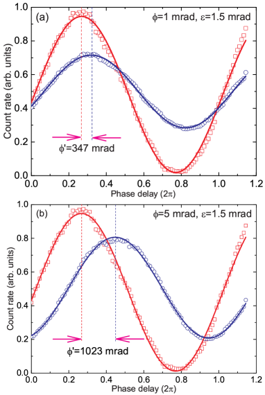
Figure 2: Measured oscillation patterns without (squares) and with (circles) weak measurement. $\varepsilon$ is set as 1.5 mrad, and $\phi$ is set as 1 mrad (a) and 5 mrad (b), respectively. By sinusoidally fitting the oscillation patterns in two cases (solid lines), the final phase shifts $\phi^{\prime}$ with weak measurement can be calculated, which are much larger than the initial phase shifts $\phi$. Such phase amplification highly depends on the parameters of $\phi$ and $\varepsilon.$

III experiment

We then perform an experiment to demonstrate the phase shift amplification based on our weak measurement scheme. The experimental setup is shown in Fig. 1. A continuous wave laser with a center wavelength of 785 nm is attenuated down to single-photon level with a set of attenuators (ATT), and the polarization state of incident photons is prepared to $\frac{1}{\sqrt{2}}(|H\rangle+|V\rangle)$ by a polarizer with PER of $\sim$ $10^{4}:1$. The initial phase shift $\phi$ between $|H\rangle$ and $|V\rangle$ to be measured is produced by a Soleil-Babinet Compensator (SBC) with a high-precision phase modulation step of $0.26$ mrad. The SBC is a zero-order retarder that can be adjusted continuously.

The weak measurement part consists of two components, a half-wave plate (HWP1) that transforms the initial state $\frac{1}{\sqrt{2}}(|H\rangle+e^{i\phi}|V\rangle)$ to $(|H\rangle+\varepsilon e^{\frac{i\phi}{2\varepsilon}}|V\rangle)/\sqrt{1+\varepsilon^{2}}$, and a Sagnac-like interferometer. $|H\rangle$ and $|V\rangle$ photons are separated into two different paths of the interferometer. Two polarizers are inserted into the transmitted and reflected paths to further improve the polarization visibility, respectively, and two attenuators are used to independently adjust the intensities of $|H\rangle$ and $|V\rangle$ photons. At the output port of the interferometer, polarization projection measurements is performed using a quarter-wave plate (QWP) set at $45^{\circ}$, HWP2, a Glan-Laser Calcite Polarizer (GL) with high PER of $\sim 10^{5}:1$, and a Silicon avalanche photodiode (APD). By tuning the angle of HWP2 to modulate the phase delay between $|H\rangle$ and $|V\rangle$, oscillation patterns are scanned, and thus the phase shifts between the oscillation patterns can be directly measured.

In the experiment, all the HWPs and polarizers are mounted on stepper electric motors, whose minimal rotation angles can reach as low as $0.52$ mrad. Fig. 2 shows the measured polarization oscillation patterns by tuning the angle of HWP2 with a phase delay step of $1^{\circ}$, and the phase shifts between the oscillation patterns are calculated using the sinusoidal fitting curves. The polarization visibility degradation as shown in Fig. 2 is mainly due to the operations of intensity balance. With $\varepsilon=$ 1.5 mrad, the final phase shifts $\phi^{\prime}$ reach 347 mrad, 1023 mrad under the settings of $\phi=$ 1 mrad, $\phi=$ 5 mrad, respectively, which clearly exhibits the phase amplification effect due to weak measurement. The phase amplification gain highly depends on the parameters of $\phi$ and $\varepsilon$. We note that without phase amplification the original phase resolution of the interferometer in the experiment using standard linear optics devices is around $10$ mrad, which is limited by the PER of GL.

Further, we investigate the quantitative relationships of three parameters, i.e., initial phase shift $\phi$, rotation angle of deviation $\varepsilon$ and final phase shift $\phi^{\prime}$. The measured results are plotted in Fig. 3. Fig. 3(a) shows the relationship between $\phi$ and $\phi^{\prime}$ with different settings of $\varepsilon$. The theoretical fitting curves are calculated according to Eq. 7. $\phi^{\prime}$ increases with the increase of $\phi$, and with a fixed value of $\phi$ rotation angles that are closer to $\pi/4$ result in larger phase shift amplification. Fig. 3 (b) shows the relationship between $\phi^{\prime}$ and $\varepsilon$ with different settings of $\phi$. $\phi^{\prime}$ decreases with the increase of $\varepsilon$, and with a fixed value of $\varepsilon$ larger initial phase shifts result in larger final phase shifts. Particularly, the slopes of phase amplification are steep in the regime of small $\varepsilon$, but become flat when $\varepsilon>$ $5$ mrad. From Fig. 3, one can find out that using weak measurement the phase resolution can be improved to $0.26$ mrad at least for the interferometer, since in the experiment the initial phase shift cannot be generated smaller than $0.26$ mrad due to the limit of SBC adjustment. This result is already significantly better than the original phase resolution of the interferometer without weak measurement. Nevertheless, in principle smaller values of $\phi$ can be resolved with our method, since the phase amplification gain is considerably high in the regime of small angles of $\varepsilon.$ For instance, with $\phi=0.26$ mrad and $\varepsilon=1.5$ mrad, the final phase shift $\phi^{\prime}$ reaches $101$ mrad, corresponding to a phase amplification gain of more than $388$.

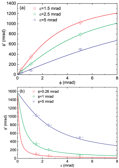
Figure 3: The plots of the final phase shifts $\phi^{\prime}$ as a function of the initial phase shift $\phi$ (a) and the rotation angle $\varepsilon$ (b). Points and solid lines represent experimental values and theoretical fits, respectively.

IV discussion

Our weak measurement scheme is compatible with the conventional approaches for phase resolution improvement in optical interferometry, especially the technique of signal proceeding, which makes it possible to perform extremely small phase measurement. For instance, an original phase shift measurement of $10^{-7}$ rad with the lock-in amplifier in an optical interferometer was reported Matsuda09 . By using the phase shifter device in that experiment instead of the SBC in our experiment and performing signal proceeding as usual, the phase amplification effect in our scheme may yield further enhancement in the phase sensitivity by 2$\sim$3 orders of magnitudes so that to bring the measurement precision of phase shift to the level of $10^{-9}$ rad.

Furthermore, our weak measurement scheme can also be adapted for $N00N$ states to achieve better phase resolution. For instance, one can prepare $N00N$ states $\frac{1}{\sqrt{2}}(|H\rangle^{\otimes n}+|V\rangle^{\otimes n})$ as input to the SBC instead of single-photon states, after projecting $n-1$ photonic qubits to $\frac{1}{\sqrt{2}}(|H\rangle\pm|V\rangle)$ as implemented in the previous $N00N$ state experiments Walther04 ; Leibfried04 ; Gao10 and performing the same unitary rotation and post-selection operation on the $n$th qubit as required in our weak measurement scheme, the final phase shift can be amplified to $\frac{n\phi}{2\varepsilon}$. The total phase uncertainty in such case is (see Eq. (A19) in Appendix A)

$$\Delta\phi=2\sqrt{\frac{\varepsilon^{2}\rho^{2}}{n^{2}}+\frac{1}{2nN}}.$$ (12)

Compared to Eq. 2, one can conclude that weak measurement scheme with $N00N$ states can not only significantly decrease the systematic phase uncertainty but also suppress the statistical phase uncertainty and particularly beat the standard quantum limit when $n>2$.

V summary

In summary, we have proposed and experimentally demonstrated direct phase shift amplification in optical interferometry with weak measurement, which drastically improves the phase shift amplification with a factor of $388$. Since phase measurement is a fundamental metrology tool, such weak measurement scheme can provide a new approach for the precision measurement applications of various physical quantities including observation of weak cross-Kerr nonlinearity Feizpour11 ; MTS17 and test of general relativity with quantum interference Zych11 .

appendix a: Phase uncertainty in interferometry with systematic error

Considering a phase measurement in a realistic interferometer, without loss of generality it is assumed that the systematic phase error $\varphi$ is a zero-mean value following a Gaussian distribution,

$$D\left(\varphi\right)\varpropto e^{-\frac{\varphi^{2}}{2\rho^{2}}},$$ (A1)

where $\rho$ is the standard derivation. The detection probability at one output port of the interferometer is

$$p=\frac{1}{2}(1+\cos(\phi+\varphi)),$$ (A2)

where $\phi$ is the phase to be measured. Given a certain fixed phase error $\varphi$, the sample size interval is $N_{\varphi}=N{\cdot}D\left(\varphi\right)\delta\varphi$. For a large total sample size $N$, the variance of estimated probability $p_{\varphi}$ in each sample interval can be calculated as

$$\left(\Delta p_{\varphi}\right)^{2}=\frac{p_{\varphi}\left(1-p_{\varphi}\right)}{N_{\varphi}}=\frac{\sin^{2}\left(\phi+\varphi\right)}{4N_{\varphi}},$$ (A3)

where $\left\langle p_{\varphi}\right\rangle=p$.

From Eq. A3, the mean values of $p$ and $p^{2}$ during the whole sampling process can be further calculated as

$$\left\langle p\right\rangle = \frac{\sum N_{\varphi}\left\langle p_{\varphi}\right\rangle}{N}\approx\int D\left(\varphi\right)\left\langle p_{\varphi}\right\rangle d\varphi$$ (A4)

$$= \frac{1}{2}+\frac{1}{2}\cos\phi\int D\left(\varphi\right)\cos\varphi d\varphi,$$

$$\left\langle p^{2}\right\rangle = \frac{\sum N_{\varphi}\left\langle p_{\varphi}^{2}\right\rangle}{N}=\frac{\sum N_{\varphi}\left[\left(\Delta p_{\varphi}\right)^{2}+\left\langle p_{\varphi}\right\rangle\right]}{N}$$ (A5)

$$\approx \frac{1}{4N}\int D\left(\varphi\right)\sin^{2}\left(\phi+\varphi\right)d\varphi$$

$$+ \frac{1}{4}\int D\left(\varphi\right)\left[1+\cos\left(\phi+\varphi\right)\right]^{2}d\varphi,$$

respectively. Combining Eq. A4 and Eq. A5, the variance of $p$ is

$$\left(\Delta p\right)^{2} = \left\langle p^{2}\right\rangle-\left\langle p\right\rangle^{2}$$ (A6)

$$= \frac{1}{4}\int\frac{1}{N}\left(\sin^{2}\phi\cos^{2}\varphi+\cos^{2}\phi\sin^{2}\varphi\right)D\left(\varphi\right)d\varphi$$

$$+ \left(\cos^{2}\phi\cos^{2}\varphi+\sin^{2}\phi\sin^{2}\varphi\right)D\left(\varphi\right)d\varphi$$

$$- \frac{1}{4}\cos^{2}\phi\left[\int\cos\varphi D\left(\varphi\right)d\varphi\right]^{2}.$$

Since $\rho\ll 1$ and $\varphi$ is a small quantity in the integrals, therefore, one can consider only the terms of $\varphi$ and $\varphi^{2}$ with the following approximations

$$\int \sin^{2}\varphi D\left(\varphi\right)d\varphi\approx\rho^{2},$$ (A7)

$$\int \cos^{2}\varphi D\left(\varphi\right)d\varphi\approx 1-\rho^{2},$$

$$\int \cos\varphi D\left(\varphi\right)d\varphi\approx 1-\frac{\rho^{2}}{2}.$$

According to Eq. A7, Eq. A6 can be simplified with approximations as

$$\left(\Delta p\right)^{2}=\frac{\sin^{2}\phi}{4}\left(\rho^{2}+\frac{1}{N}+\frac{\cos^{2}\phi\rho^{2}}{N\sin^{2}\phi}\right).$$ (A8)

Combining Eq. A2 and Eq. A8, the phase uncertainty is calculated as

$$\Delta\phi = \left|\frac{d\phi}{dp}\cdot\Delta p\right|$$ (A9)

$$= \sqrt{\rho^{2}+\frac{1}{N}+\frac{\rho^{2}}{N\sin^{2}\phi}}.$$

Due to the existence of phase errors, the theoretically maximum estimated probability is $1-\frac{1}{N}$. From Eq. A2, one can calculate the minimum measurable phase by $\sin^{2}\phi=\frac{4}{N}$. Therefore, the phase uncertainty in a realistic interferometer can be roughly estimated as

$$\Delta\phi=\sqrt{\rho^{2}+\frac{1}{N}}.$$ (A10)

Further, one can calculate the phase uncertainty in the following cases, i.e., using $N00N$ state, using single-qubit state with weak measurement and using $N00N$ state with weak measurement.

$N00N$ state. With a sample size $m$ satisfying $n\cdot m=N$, the detection probability at one output port of an interferometer is

$$p^{(N)}=\frac{1}{2}\left(1+\cos\left(n\phi+\varphi\right)\right).$$ (A11)

The mean value and the variance of estimated probability in each sampling interval are

$$\left\langle p_{\varphi}^{(N)}\right\rangle = p^{(N)},$$

$$\left(\Delta p_{\varphi}^{(N)}\right)^{2} = \frac{n\sin^{2}\left(n\phi+\varphi\right)}{4N_{\varphi}},$$ (A12)

respectively. Therefore, the phase uncertainty using $N00N$ states in a realistic interferometer is

$$\Delta\phi=\sqrt{\frac{\rho^{2}}{n^{2}}+\frac{1}{nN}}.$$ (A13)

Single-qubit state with weak measurement. As described in the text, in such case the detection probability at one output port of an interferometer is

$$p_{W}=\frac{1}{2}\left(1+\cos\left(\frac{\phi}{2\varepsilon}+\varphi\right)\right),$$ (A14)

with a sample size of $2\varepsilon^{2}N$. Then, the mean value and the variance of estimated probability in each sampling interval are

$$\left\langle p_{\varphi W}\right\rangle = p_{W},$$

$$\left(\Delta p_{\varphi W}\right)^{2} = \frac{\sin^{2}\left(\frac{\phi}{2\varepsilon}+\varphi\right)}{2\varepsilon^{2}N_{\varphi}},$$ (A15)

respectively. Therefore, the phase uncertainty using single-qubit states with weak measurement in a realistic interferometer is

$$\Delta\phi=2\sqrt{\varepsilon^{2}\rho^{2}+\frac{1}{2N}}.$$ (A16)

$N00N$ state with weak measurement. As described in the text, in such case the detection probability at one output port of an interferometer is

$$p_{W}^{(N)}=\frac{1}{2}\left(1+\cos\left(\frac{n\phi}{2\varepsilon}+\varphi\right)\right),$$ (A17)

with a sample size of $\frac{2\varepsilon^{2}N}{n}$. Then, the mean value and the variance of estimated probability in each sampling interval are

$$\left\langle p_{\varphi W}^{(N)}\right\rangle = p_{W}^{(N)},$$

$$\left(\Delta p_{\varphi W}^{(N)}\right)^{2} = \frac{n\sin^{2}\left(\frac{n\phi}{2\varepsilon}+\varphi\right)}{2\varepsilon^{2}N_{\varphi}},$$ (A18)

respectively. Therefore, the phase uncertainty using $N00N$ states with weak measurement in a realistic interferometer is

$$\Delta\phi=2\sqrt{\frac{\varepsilon^{2}\rho^{2}}{n^{2}}+\frac{1}{2nN}}.$$ (A19)

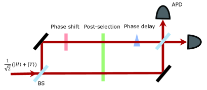
Figure 4: Phase amplification scheme with standards weak measurement. In the upper path of the interferometer, a tiny phase shift $\phi$ is induced between $|H\rangle$ and $|V\rangle$. The post-selection is set to the almost orthogonal state of the incident polarization states. The tunable phase delay in the path is used to measure the oscillation patterns.

appendix b: Phase amplification scheme with standard weak measurements

In this scheme, the polarization degree of freedom can be treated as a system, and the path degree of freedom can be treated as a qubit meter.

As shown in Fig. 4, the initial system and meter state are $|i\rangle=\frac{1}{\sqrt{2}}(|H\rangle+|V\rangle)$ and $\frac{1}{\sqrt{2}}(|0\rangle+|1\rangle)$, respectively, where the $|0\rangle$ and $|1\rangle$ are labels of the upper and lower paths of Mach-Zehnder interferometer. Given a tiny phase shift $\phi$ between $|H\rangle$ and $|V\rangle$ in the path $|0\rangle$ to be measured, the system-meter composite state is

$$\frac{1}{2}[|H\rangle(|0\rangle+e^{i\phi/2}|1\rangle)+|V\rangle(|0\rangle+e^{-i\phi/2}|1\rangle)].$$ (A20)

Therefore, the coupling of the system and meter can be written as

$$\frac{1}{2}e^{-\frac{i\phi}{4}\sigma_{z}\otimes\sigma_{z}}\left(|H\rangle+|V\rangle\right)\otimes\left(|0\rangle+|1\rangle\right),$$ (A21)

where $\phi\ll 1$ shows the weak interaction. Then, the system state is post-selected to the almost orthogonal final state $|f\rangle=\sin(\pi/4+\varepsilon)|H\rangle-\cos(\pi/4+\varepsilon)|V\rangle$ ($\varepsilon\ll 1$) in both paths. When $\phi/\varepsilon\ll 1,$ the final meter state is approximately

$$\frac{1}{\sqrt{2}}\left\langle f\right|\left(1-\frac{i\phi}{4}\sigma_{z}\otimes\sigma_{z}\right)|i\rangle\otimes\left(|0\rangle+|1\rangle\right)$$ (A22)

$$\approx \frac{\left\langle f|i\right\rangle}{\sqrt{2}}e^{\frac{-i\phi\left\langle f\right|\sigma_{z}\left|i\right\rangle}{4\left\langle f|i\right\rangle}\sigma_{z}}\left(|0\rangle+|1\rangle\right)$$

$$= \frac{\left\langle f|i\right\rangle}{\sqrt{2}}\left(|0\rangle+e^{\frac{i\phi}{2\varepsilon}}|1\rangle\right),$$

where the weak value is $A_{W}\equiv\frac{\left\langle f\right|\sigma_{z}\left|i\right\rangle}{\left\langle f|i\right\rangle}\approx\frac{1}{\varepsilon}$ and the successful probability is $\left|\left\langle f|i\right\rangle\right|^{2}\approx$ $\varepsilon^{2}.$

References

- (1) V. Giovannetti, S. Lloyd, and L. Maccone, Science 306, 1330-1336 (2004).
- (2) V. Giovannetti, S.Lloyd, and L. Maccone, Nat. Photon. 5, 222-229 (2011).
- (3) A. Boto, P. Kok, D. S. Abrams, S. L. Braunstein, C. P. Williams, and J. P. Dowling, Phys. Rev. Lett. 85, 2733-2736 (2000).
- (4) M. J. Holland and K. Burnett, Phys. Rev. Lett. 71, 1355-1358 (1993).
- (5) C. M. Caves, Phys. Rev. D 23, 1693-1708 (1981).
- (6) X.-L. Wang, L.-K. Chen, W. Li, H.-L. Huang, C. Liu, C. Chen, Y.-H. Luo, Z.-E. Su, D. Wu, Z.-D. Li, H. Lu, Y. Hu, X. Jiang, C.-Z. Peng, L. Li, N.-L. Liu, Y.-A. Chen, C.-Y. Lu, and J.-W. Pan, Phys. Rev. Lett. 117, 210502 (2016).
- (7) L.-K. Chen, Z.-D. Li, X.-C. Yao, M. Huang, W. Li, H. Lu, X. Yuan, Y.-B. Zhang, X. Jiang, C.-Z. Peng, L. Li, N.-L. Liu, X. Ma, C.-Y. Lu, Y.-A. Chen, and J.-W. Pan, Optica 4, 77-83 (2017).
- (8) Y. Aharonov, D. Z. Albert, and L. Vaidman, Phys. Rev. Lett. 60, 1351-1354 (1988).
- (9) Y. Aharonov and L. Vaidman, Phys. Rev. A 41, 11-20 (1990).
- (10) A. Feizpour, X. Xing, and A. M. Steinberg, Phys. Rev. Lett. 107, 133603 (2011).
- (11) O. Zilberberg, A. Romito, and Y. Gefen, Phys. Rev. Lett. 106, 080405 (2011).
- (12) S. Wu and M. Zukowski, Phys. Rev. Lett. 108, 080403 (2012).
- (13) G. Strübi and C. Bruder, Phys. Rev. Lett. 110, 083605 (2013).
- (14) S. Pang, J. Dressel, and T. A. Brun, Phys. Rev. Lett. 113, 030401 (2014).
- (15) O. Hosten and P. Kwiat, Science 319, 787-790 (2008).
- (16) P. B. Dixon, D. J. Starling, A. N. Jordan, and J. C. Howell, Phys. Rev. Lett. 102, 173601 (2009).
- (17) Y. Gorodetski, K. Y. Bliokh, B. Stein, C. Genet, N. Shitrit, V. Kleiner, E. Hasman, and T. W. Ebbesen, Phys. Rev. Lett. 109, 013901 (2012).
- (18) O. S. Magaña-Loaiza, M. Mirhosseini, B. Rodenburg, and R. W. Boyd, Phys. Rev. Lett. 112, 200401 (2014).
- (19) N. Brunner and C. Simon, Phys. Rev. Lett. 105, 010405 (2010).
- (20) X.-Y. Xu, Y. Kedem, K. Sun, L. Vaidman, C.-F. Li, and G.-C. Guo, Phys. Rev. Lett. 111, 033604 (2013).
- (21) L. J. Salazar-Serrano, D. Janner, N. Brunner, V. Pruneri, and J. P. Torres, Phys. Rev. A 89, 012126 (2014).
- (22) X. Qiu, L. Xie, X. Liu, L. Luo, Z. Li, Z. Zhang, and J. Du, Appl. Phys. Lett. 110, 071105 (2017).
- (23) S. Wu and K. Mølmer, Phys. Lett. A 374, 34-39 (2009).
- (24) N. Matsuda, R. Shimizu, Y. Mitsumori, H. Kosaka, and K. Edamatsu, Nat. Photon. 3, 95-98 (2009).
- (25) P. Walther, J.-W. Pan, M. Aspelmeyer, R. Ursin, S. Gasparoni, and A. Zeilinger, Nature 429, 158-161 (2004).
- (26) D. Leibfried, M. D. Barrett, T. Schaetz, J. Britton, J. Chiaverini, W. M. Itano, J. D. Jost, C. Langer, and D. J. Wineland, Science 304, 1476-1478 (2004).
- (27) W.-B. Gao, C.-Y. Lu, X.-C. Yao, P. Xu, O. Gühne, A. Goebel, Y.-A. Chen, C.-Z. Peng, Z.-B. Chen, and J.-W. Pan, Nat. Phys. 6, 331-335 (2010).
- (28) F. Matsuoka, A. Tomita, and Y. Shikano, Quantum Stud.: Math. Found. 4, 159-169 (2017).
- (29) M. Zych, F. Costa, I. Pikovski, and C. Brukner, Nat. Commun. 2, 505 (2011).