The $\rm HI$- and $\rm H_{2}$-to-stellar mass correlations of late- and early-type galaxies and their consistency with the observational mass functions

Abstract

We compile and carrefully homogenize local galaxy samples with available information on stellar, $\rm HI$ and/or $\rm H_{2}$ masses, and morphology. After processing the information on upper limits in the case of non gas detections, we determine the $\rm HI$- and $\rm H_{2}$-to-stellar mass relations and their $1\sigma$ scatter for both late- and early-type galaxies. The obtained relations are fitted to single or double power laws. Late-type galaxies are significantly gas richer than early-type ones, specially at high masses. The respective $\rm H_{2}$-to-$\rm HI$ mass ratios as a function of $M_{*}$ are discussed. Further, we constrain the full mass-dependent distribution functions of the $\rm HI$- and $\rm H_{2}$-to-stellar mass ratios. We find that they can be described by a Schechter function for late types and a (broken) Schechter + uniform function for early types. By using the observed galaxy stellar mass function and the volume-complete late-to-early-type galaxy ratio as a function of $M_{*}$, these empirical distribution functions are mapped into $\rm HI$ and $\rm H_{2}$ mass functions. The obtained mass functions are consistent with those inferred from large surveys. The empirical gas-to-stellar mass relations and their distributions for local late- and early-type galaxies presented here can be used to constrain models and simulations of galaxy evolution.

Compilamos y homogeneizamos muestras locales de galaxias que contienen información de la masa estelar, de $\rm HI$ y/o $\rm H_{2}$, y morfología. Procesamos adecuadamente la información relacionada con las no detecciones en gas y determinamos la relaciones de masa estelar a masa de $\rm HI$ y $\rm H_{2}$ y sus dispersiones, tanto para galaxias tardías como tempranas. Las relaciones se describen por leyes simples o doble de potencias; las respectivos cocientes de masa $\rm H_{2}$ a $\rm HI$ son presentados. Contreñimos también las distribuciones completas de los cocientes de masa de $\rm HI$ y $\rm H_{2}$ a masa estelar, encontrando que se describen bien por una función de Schechter (galaxias tardías) y una función Schechter (cortada) + uniforme (galaxias tempranas). Usando la función de masa estelar y el cociente de galaxias tempranas a tardías en función de $M_{*}$, estas distribuciones son mapeadas en funciones de masa de $\rm HI$ y $\rm H_{2}$. Las funciones de masa obtenidas son consistentes con aquellas inferidas de catastros. Las relaciones empíricas de masa de gas a estrellas y sus distribuciones para galaxias tardías/tempranas presentadas aquí pueden ser usadas para constreñir modelos y simulaciones de evolución de galaxias.

galaxies: general galaxies: ISM galaxies: mass functions galaxies: statistics

0.1 Introduction

Galaxies are complex systems, formed mainly from the cold gas captured by the gravitational potential of dark matter halos and transformed into stars, but also reheated and eventually ejected from the galaxy by feedback processes (see for a recent review Somerville & Davé, 2015). Therefore, the content of gas, stars, and dark matter of galaxies provides key information to understand their evolution and present-day status, as well as to constrain models and simulations of galaxy formation (see e.g., Zhang et al., 2009; Fu et al., 2010; Lagos et al., 2011; Duffy et al., 2012; Lagos et al., 2015).

Local galaxies fall into two main populations, according to the dominion of the disk or bulge component (late- and early-types, respectively; a strong segregation is also observed by color or star formation rate). The main properties and evolutionary paths of these components are different. Therefore, the present-day stellar, gaseous, and dark matter fractions are expected to be different among late-type/blue/star-forming and early-type/red/passive galaxies of similar masses. The above demands the gas-to-stellar mass relations to be determined separately for each population. Morphology, color and star formation rate correlate among them, though there is a fraction of galaxies that skips the correlations. In any case, when only two broad groups are used to classify galaxies, the segregation in the resulting correlations for each group is expected to be similar for any of these criteria. Here we adopt the morphology as the criterion for classifying galaxies into two broad populations.

With the advent of large homogeneous optical/infrared surveys, the statistical distributions of galaxies, for example the galaxy stellar mass function (GSMF), are very well determined now. In the last years, using these surveys and direct or statistical methods, the relationship between the stellar, $M_{*}$, and halo masses has been constrained (e.g., Mandelbaum et al., 2006; Conroy & Wechsler, 2009; More et al., 2011; Behroozi et al., 2010; Moster et al., 2010; Rodríguez-Puebla et al., 2013; Behroozi et al., 2013; Moster et al., 2013; Zu & Mandelbaum, 2015). Recently, the stellar-to-halo mass relation has been even inferred for (central) galaxies separated into blue and red ones by Rodríguez-Puebla et al. (2015). These authors have found that there is a segregation by color in this relation (see also Mandelbaum et al., 2016). The semi-empirical stellar-to-halo mass relation and its scatter provide key constraints to models and simulations of galaxy evolution. These constraints would be stronger if the relations between the stellar and atomic/molecular gas contents of galaxies are included. With this information, the galaxy baryonic mass function can be also constructed and the baryonic-to-halo mass relation can be inferred, see e.g, Baldry et al. (2008).

While the stellar component is routinely obtained from large galaxy surveys in optical/infrared bands, the information about the cold gas content is much more scarce due to the limits in sensitivity and sky coverage of current radio telescopes. In fact, the few blind $\rm HI$ surveys, obtained with a fixed integration time per pointing, suffer of strong biases, and for $\rm H_{2}$ (CO) there are not such surveys. For instance, the $\rm HI$ Parkes All-Sky Survey (HIPASS; Barnes et al., 2001; Meyer et al., 2004) or the Arecibo Legacy Fast ALFA survey (ALFALFA; Giovanelli et al., 2005; Haynes et al., 2011; Huang et al., 2012a), miss galaxies with low gas-to-stellar mass ratios, specially at low stellar masses. Therefore, the $\rm HI$-to-stellar mass ratios inferred from the crossmatch of these surveys with optical ones should be regarded as an upper limit envelope (see e.g., Baldry et al., 2008; Papastergis et al., 2012; Maddox et al., 2015). In the future, facilities as the Square Kilometre Array (SKA; Carilli & Rawlings, 2004; Blyth et al., 2015) or precursor instruments as the Australian SKA Pathfinder (ASKAP; Johnston et al., 2008) and the outfitted Westerbork Synthesis Radio Telescope (WSRT), will bring extragalactic gas studies more in line with optical surveys. Until then, the gas-to-stellar mass relations of galaxies can be constrained: i) from limited studies of radio follow-up observations of large optically-selected galaxy samples or by cross-correlating some radio surveys with optical/infrared surveys (e.g., Catinella et al., 2012; Saintonge et al., 2011; Boselli et al., 2010; Papastergis et al., 2012); and ii) from model-dependent inferences based, for instance, on the observed metallicities of galaxies or from calibrated correlations with photometrical properties (e.g., Baldry et al., 2008; Zhang et al., 2009).

While this paper does not present new observations, it can be considered as an extension of previous efforts in attempting to determine the $\rm HI$-, $\rm H_{2}$- and cold gas-to-stellar mass correlations of local galaxies over a wide range of stellar masses. Moreover, here we separate galaxies into at least two broad populations, late- and early-type galaxies (hereafter LTGs and ETGs, respectively). These empirical correlations are fundamental benchmarks for models and simulations of galaxy evolution. Our main goal here is to constrain these correlations by using and uniforming large galaxy samples of good quality radio observations with confirmed optical counterparts. Moreover, the well determined local GSMF combined with these correlations can be used to construct the galaxy $\rm HI$ and $\rm H_{2}$ mass functions, G$\rm HI$MF and G$\rm H_{2}$MF, respectively. As a test of consistency, we compare these mass functions with those reported in the literature for $\rm HI$ and CO ($\rm H_{2}$).

Many of the samples compiled here suffer of incompleteness and selection effects or in many cases the radio observations provide only upper limits to the flux (non detections). To provide reliable determinations of the $\rm HI$- and $\rm H_{2}$-to-stellar mass correlations, for both LTGs and ETGs, here we homogenize as much as possible the data, check them against selection effects that could affect the calibration of the correlations, and take into account the upper limits adequately. We are aware on the limitations of this approach. Note, however, that in absence of large homogeneous galaxy surveys reporting gas scaling relations over a wide dynamical range and separated into late- and early-type galaxies, the above approach is well supported as well as their, fair, use.

The plan of the paper is as follows. In Section 0.2 and Appendices .9 and .10, we present our compilation and homogenization of local galaxy samples from the literature with available information on stellar mass, morphological type, and $\rm HI$ and/or $\rm H_{2}$ masses. In Section 0.3, we test the different compiled samples against possible biases in the gas contents due to selection effects. In Section 0.4, we describe the strategy to infer the gas-to-stellar mass correlations taking into account upper limits, and present the determination of these correlations for the LTG and ETG populations (mean and standard deviations). Further, in Section 0.5 we constrain the full distributions of the gas-to-stellar mass ratios as a function of $M_{*}$. In Section 0.6 we explore the consistency of the determined correlations with the observed $\rm HI$ and $\rm H_{2}$ mass functions, by using the GSMF as an interface. In subsection 0.7.1 we discuss the $\rm H_{2}$-to-$\rm HI$ mass ratios of LTGs and ETGs inferred from our correlations; subsection 0.7.2 is devoted to a discussion on the role of environment, and subsection 0.7.3 presents comparisons with some previous attempts to determine the gas scaling relations. A summary of our results and the conclusions are presented in Section 0.8. Finally, Table 1 lists all the acronyms used in this paper, including the ones of the surveys/catalogs used here.

Table 1: List of acronyms used in this paper

BCD	Blue compact dwarf
ETG	Early-type galaxy
G$\rm HI$MF	Galaxy $\rm HI$ Mass Function
G$\rm H_{2}$MF	Galaxy $\rm H_{2}$ Mass Function
GSMF	Galaxy Stellar Mass Function
IMF	Initial Mass Function
LTG	Late-type galaxy
MW	Milky Way
$R_{\rm HI}$ and $R_{\rm H_{2}}$	$\rm HI$- and $\rm H_{2}$-to stellar mass ratio
SB	Surface brightness
SFR	Star formation rate
ALFALFA	Arecibo Legacy Fast ALFA survey
ALLSMOG	APEX Low-redshift Legacy Survey for MOlecular Gas
AMIGA	Analysis of the interstellar Medium of Isolated GAlaxies
ASKAP	Australian SKA Pathfinder
ATLAS3D	(A volume-limited survey of local ETGs)
COLD GASS	CO Legacy Database for GASS
FCRAO	Five College Radio Astronomy Observatory
GALEX	Galaxy Evolution EXplorer
GAMA	Galaxy And Mass Assembly
GASS	GALEX Arecibo SDSS Survey
HERACLES	HERA CO-Line Extragalactic Survey
HIPASS	$\rm HI$ Parkes All-Sky Survey
HRS	Herschel Reference Survey
NFGS	Nearby Field Galaxy Catalog
NRTA	Nancay Radio Telescope
SDSS	Sloan Digital Sky Survey
SINGS	Spitzer Infrared Nearby Galaxies Survey
SKA	Square Kilometre Array
THINGS	The $\rm HI$ Nearby Galaxy Survey
UNAM-KIAS	UNAM-KIAS survey of SDSS isolated galaxies
UNGC	Updated Nearby Galaxy Catalog
WRST	Westerbork Synthesis Radio Telescope

0.2 Compilation of Observational Data

The main goal of this Section is to present our extensive compilation of observational studies (catalogs, surveys or small samples) that meet the following criteria:

• Include $\rm HI$ and/or $\rm H_{2}$ masses from radio observations, and luminosities/stellar masses from optical/infrared observations.

• Provide the galaxy morphological type or a proxy of it.

• Describe the selection criteria of the sample and provide details about the radio observations, flux limits, etc.

• Include individual distances to the sources and corrections for peculiar motions/large-scale structures for the nearby galaxies.

• In the case of non-detections, provide estimates of the upper limits for $\rm HI$ or $\rm H_{2}$ masses.

The observational samples that meet the above criteria are listed in Table 2. In Appendices .9 and .10, we present a summary of each one of them. We have found information on colors ($g-r$ or $B-K$) for most of the samples. For $\mbox{$M_{*}$}>10^{9}$ M_⊙, the galaxies in the color–mass diagram segregate into the so-called red sequence and blue cloud. Excluding those more inclined than 70 degrees, we find that $\sim 83\%$ of LTGs ($\sim 80\%$ of ETGs) have colors that can be classified as blue (red) by using a mass-dependent $(g-r)$ criterion for defining blue/red galaxies. At masses lower than $\mbox{$M_{*}$}\approx 10^{9}$ M_⊙, the overwhelming majority of galaxies are of late types and classify as blue.

Table 2: Observational samples

Sample	Selection	Environment	$\rm HI$	Detections / Total	$\rm H_{2}$	Detections / Total	IMF	Category
UNGC	ETG+LTG	local 11 Mpc	Yes	407 / 418	No	–	diet-Salpeter	Gold
GASS/COLD GASS	ETG+LTG	no selection	Yes	511 / 749	Yes	229 / 360	Chabrier (2003)	Gold
HRS–field	ETG+LTG	no selection	Yes	199 / 224	Yes	101 / 156	Chabrier (2003)	Gold
ATLAS3D–field	ETG	field	Yes	51 / 151	Yes	55 / 242	Kroupa (2001)	Gold
NFGS	ETG+LTG	no selection	Yes	163 / 189	Yes	27 / 31	Chabrier (2003)	Silver
Stark et al. (2013) compilation∗	LTG	no selection	Yes	62/62	Yes	14 / 19	diet-Salpeter	Silver
Leroy+08 THINGS/HERACLES	LTG	nearby	Yes	23 / 23	Yes	18 / 20	Kroupa (2001)	Silver
Dwarfs-Geha+06	LTG	nearby	Yes	88 / 88	No	–	Kroupa et al. (1993)	Silver
ALFALFA dwarf	ETG+LTG	no selection	Yes	57 / 57	No	–	Chabrier (2003)	Silver
ALLSMOG	LTG	field	No	–	Yes	25 / 42	Kroupa (2001)	Silver
Bauermeister et al. (2013) compilation	LTG	field	No	–	Yes	7 / 8	Kroupa (2001)	Silver
ATLAS3D–Virgo	ETG	Virgo core	Yes	2 / 15	Yes	4 / 21	Kroupa (2001)	Bronze
AMIGA	ETG+LTG	isolated	Yes	229 / 233	Yes	158 / 241	diet-Salpeter	Bronze
HRS–Virgo	ETG+LTG	Virgo core	Yes	55 / 82	Yes	36 / 62	Chabrier (2003)	Bronze
UNAM-KIAS	ETG+LTG	isolated	Yes	352 / 352	No	–	Kroupa (2001)	Bronze
Dwarfs-NSA	LTGs	isolated	Yes	124 / 124	No	–	Chabrier (2003)	Bronze

• ^∗ From this compilation, we considered only galaxies that were not in GASS, COLD GASS and ATLAS^3D samples.

0.2.1 Systematical Effects on the $\rm HI$- and $\rm H_{2}$-to-stellar mass correlations

To reduce potential systematical effects that can bias how we derive the $\rm HI$- and $\rm H_{2}$-to-stellar mass correlations we homogenize all the compiled observations to a same basis. Following, we discuss some potential sources of bias/segregation and the calibration that we apply to the observations. It is important to stress that for inferring scaling correlations, as those of the gas fraction as a function of stellar mass, what is important is to have a statistically representative and not biased population of galaxies at each mass bin. Thus, it is not a need to have mass limited volume-complete samples (see also subsection 0.4.1). However, a volume-complete sample assures that possible biases on the measure in question due to selection functions in galaxy type, color, environment, surface brightness, etc., are not introduced. The main expected bias in the gas content at a given stellar mass is due to the galaxy type/color; this is why we need to separate the samples at least into two broad populations, LTGs and ETGs.

Galaxy type

The gas content of galaxies, at a given $M_{*}$, segregates significantly with galaxy morphological type (e.g., Kannappan et al., 2013; Boselli et al., 2014c). Thus, information on morphology is necessary in order to separate galaxies at least into two broad populations, LTGs and ETGs. Besides of its physical basis, this separation is important for not introducing biases in the obtained correlations due to selection effects related to the morphology in the different samples used here. For example, some samples are only for late-type or star-forming galaxies, others only for early-type galaxies, etc., so that by combining them without a separation by morphology would yield correlations that are not statistically representative. We consider ETGs those classified as ellipticals (E), lenticulars (S0), dwarf E, and dwarf spheroidals or with $T<1$, and LTGs those classified as Spirals (S), Irregulars (Irr), dwarf Irr, and blue compact dwarfs or with $T\geq 1$. The morphological classification criteria used in the different samples are diverse, from individual visual evaluation to automatic classification methods as the one by Huertas-Company et al. (2011). We are aware of the high level of uncertainty introduced by using different morphological classification methods. However, in our case the morphological classification is used for separating galaxies just into two broad groups. Therefore, such an uncertainty is not expected to affect significantly any of our results. It is important to highlight that the terms LTG and ETG are useful only as qualitative descriptors. These descriptors should not be applied to individual galaxies, but instead to two distinct populations of galaxies in a statistical sense.

Environment

The gas content of galaxies is expected to depend on environment (e.g., Zwaan et al., 2005; Geha et al., 2012; Jones et al., 2016; Brown et al., 2017). In this study we are not in position of studying in detail such a dependence, though our separation into LTG and ETG populations partially takes into account this dependence because these populations segregate by environment (e.g., Dressler, 1980; Kauffmann et al., 2004; Blanton et al., 2005a; Blanton & Moustakas, 2009, and more references therein). In any case, in our compilation we include three samples specially selected to contain very isolated galaxies and one subsample of galaxies from the Virgo Cluster central regions. We will check whether their $\rm HI$ and $\rm H_{2}$ mass fractions significantly deviate or not from the mean relations.

Systematical Uncertainties on the Stellar Masses

There are many sources of systematic uncertainty in the inference of the stellar masses related to the choices of: initial mass function (IMF), stellar population synthesis and dust attenuation models, star formation history parametrization, metallicity, filter setup, etc. For inferences from broad-band spectral energy distribution fitting and using a large diversity of methods and assumptions, Pforr et al. (2012) estimate a maximal variation in stellar mass calculations of $\sim 0.6$ dex. The major contribution to these uncertainties comes from the IMF. The IMF can introduce a systematical variation up to $\approx 0.25$ dex (see e.g., Conroy, 2013). For local normal galaxies and from UV/optical/IR data (as it is the case of our compiled galaxies), Moustakas et al. (2013) find a mean systematic differences between different mass-to-luminosity estimators (fixed IMF) less than $0.2$ dex. We have seen that in most of the samples compiled here, the stellar masses are calculated using roughly similar mass-to-luminosity estimators, but the IMF are not always the same.Therefore, we homogenize the reported stellar masses in the different compiled samples to the mass corresponding to a Chabrier (2003) initial mass function (IMF), and neglect other sources of systematic differences.

Other effects

We also homogenize the distances to the value of $H_{0}=70$ kms^-1 Mpc^-1. In most of the samples compiled here (at least the most relevant ones for our study), distances were corrected for peculiar motions and large-scale structure effects. When the authors included helium and metals to their reported $\rm HI$ and $\rm H_{2}$ masses, we take care in subtracting these contributions. When we calculate the total cold gas mass, then helium and metals are explicitly taken into account.

Categories

The different $\rm HI$ and $\rm H_{2}$ samples used in this paper are wide in diversity, in particular they were obtained with different selection functions, radio telescopes, exposure times, etc. We have divided the different samples into three categories according to the feasibility of each one for determining robust and statistically representative $\rm HI$- or $\rm H_{2}$-to-stellar mass correlations for the LTG and ETG populations. We will explore whether the less feasible categories should be included or not for determining these correlations. The three categories are:

1. Golden: It includes datasets based on volume-complete (above a given luminosity/mass) samples or on representative galaxies selected from volume-complete samples. The Golden datasets, by construction, are unbiased samples of the galaxy properties distribution.

2. Silver: It includes datasets from galaxy samples that are not volume complete but that are attempted to be statistically representative at least for their morphological groups, i.e., these samples do not present obvious or strong selection effects.

3. Bronze: This category is for samples selected deliberately by environment, and it will be used to explore the effects of environment on the LTG and ETG $\rm HI$- or $\rm H_{2}$-to-stellar mass correlations.

0.2.2 The compiled $\rm HI$ sample

Table 3: Number of galaxies with detections and upper limits by morphology

Morphology(%)	Detections(%)	Upper limits(%)	Total
$\rm HI$ data
LTG (78%)	1975 (94%)	121 (6%)	2096
ETG (22%)	292 (50%)	288 (50%)	580
$\rm H_{2}$ data
LTG (63%)	533 (75%)	180 (25%)	713
ETG (37%)	124 (29%)	298 (71%)	422

Table 4: Number of galaxies with detections and upper limits by category

Category (%)	Detections (%)	Upper limits (%)	Total
$\rm HI$ data
Golden (58%)	1168 (76%)	374 (24%)	1542
Silver (16%)	391 (94%)	26 (6%)	417
Bronze (26%)	708 (99%)	9 (1%)	717
$\rm H_{2}$ data
Golden (67%)	385 (51%)	373 (49%)	758
Silver (10%)	91 (76%)	29 (24%)	120
Bronze (23%)	181 (70%)	76 (30%)	257

Appendix .9 presents a summary of the $\rm HI$ samples compiled in this paper (see also Table 2). Table 3 lists the total numbers and fractions of compiled galaxies with detection and non detection for each galaxy population. Table 4 lists the number of detected and non-detected galaxies for the golden, silver, and bronze categories listed above (§§0.2.1).

Figure 1 shows the mass ratio $\mbox{$R_{\rm HI}$}\equiv\mbox{$M_{HI}$}/\mbox{$M_{*}$}$ vs. $M_{*}$ for the compiled samples. Note that we have applied some corrections to the reported samples (see above) to homogenize all the data. The upper and bottom left panels of Figure 1 show, respectively, the compilations for LTGs and ETGs. The different symbols indicate the source reference of the data and the downward arrows are the corresponding upper limits on the $\rm HI$-flux for non-detections. We also reproduce the mean and standard deviation in different mass bins as reported in Maddox et al. (2015) for a cross-match of the ALFALFA and SDSS surveys. As mentioned in the Introduction, the ALFALFA survey is biased to high $R_{\rm HI}$ values, specially towards the low mass side. Note that the small ALFALFA subsample of dwarf galaxies by Huang et al. (2012b, dark purple dots) was selected namely as an attempt to take into account low-$\rm HI$ mass galaxies in the low-mass end.

Figure 1: Atomic gas-to-stellar mass ratio as a function of $M_{*}$. Upper panels: Compiled and homogenized data with information on $R_{\rm HI}$ and $M_{*}$ for LTGs (the different sources are indicated inside the left panel; see Appendix .9 for the acronyms and authors); downward arrows show the reported upper limits for non detections. The blue triangles with thin error bars are mean values and standard deviations from the v.40 ALFALFA and SDSS crossmatch according to Maddox et al. (2015); the ALFALFA galaxies are biased to high values of $R_{\rm HI}$ (see text). Right panel is the same as left one, but with the data separated into three categories: Golden, Silver, and Bronze (yellow, gray, and brown symbols, respectively). The red and blue lines are Buckley-James linear regressions (taking into account non-detections) for the high- and low-mass sides, respectively; the dotted lines show extrapolations from these fits. Squares with error bars are the mean and standard deviation of the data in different mass bins, taking into account non-detections by means of the Kaplan-Meier estimator. Open circles with error bars are the corresponding median and 25-75 percentiles. Estimates of the observational uncertainties are showed in the panel corners (see text). Lower panels: Same as in upper panels but for ETGs. In the right panel, we have corrected by distance the galaxies with upper limits from GASS to make them consistent with the distances of the ATLAS^3D sample (see text), and the upper limits from the latter, where increased by a factor of two to homogenize them to the ALFALFA instrument and signal-to-noise criteria. For the bins where more than 50% of the data are upper limits, the median and percentiles are not calculated.

0.2.3 The compiled $\rm H_{2}$ sample

Since the emission of cold $\rm H_{2}$ in the ISM is extremely weak, a tracer of the $\rm H_{2}$ abundance should be used. The best tracer from the observational point of view is the CO molecule due to its relatively high abundance and its low excitation energy. The $\rm H_{2}$ mass is related to the CO luminosity through a $\rm CO\mbox{-to-}H_{2}$ conversion factor: $\mbox{$M_{H_{2}}$}=\alpha_{\mbox{\tiny CO}}L_{\mbox{\tiny CO}}$. This factor has been determined in molecular clouds in the Milky Way (MW), $\alpha_{\mbox{\tiny CO,MW}}=3.2$ (K km s^-1 pc^-1)^-1, with a systematic uncertainty of $30$%. It was common to assume that this conversion factor is the same for all galaxies. However, several pieces of evidence show that $\alpha_{\rm CO}$ is not constant, and it depends mainly on the gas-phase metallicity, increasing as the galaxy metallicity decreases (e.g., Boselli et al., 2002; Schruba et al., 2012; Narayanan et al., 2012; Bolatto et al., 2013, and more references therein). As first-order, $\alpha_{\rm CO}$ changes slowly for metallicities larger than $12+\log_{10}(\mbox{O}/\mbox{H})\sim 8.4$ (approximately half the solar one) and increases considerably as the metallicity decreases. Here, we combine the dependence of $\alpha_{\rm CO}$ on metallicity given by Wolfire et al. (2010) and the observed mass–metallicity relation to obtain an approximate estimation of the dependence of $\alpha_{\rm CO}$ on $M_{*}$ for LTGs; see Appendix .11 for details. We are aware that the uncertainties involved in any metallicity-dependent correction remain substantial (Bolatto et al., 2013). Note, however, that our aim is to introduce and explore at a statistical level a reasonable mass-dependent correction to the $\rm CO\mbox{-to-}H_{2}$ factor, which must be better than ignoring it. In any case, we present results both for $\mbox{$\alpha_{\rm CO}$}=\alpha_{\mbox{\tiny CO,MW}}$ and our inferred mass-dependent $\alpha_{\rm CO}$ factor. In fact, the mass-dependent factor is important only for LTGs with $\mbox{$M_{*}$}<\lesssim 3\times 10^{10}$ M_⊙; for higher masses and for all ETGs, $\mbox{$\alpha_{\rm CO}$}\approx\alpha_{\mbox{\tiny CO,MW}}$

Appendix .10 presents a description of the CO ($\rm H_{2}$) samples that we utilize in this paper. Table 3 lists the number of galaxies with detections and upper limits of the compilation sample in terms of morphology. Table 4 lists the number of detections and upper limits for the golden, silver, and bronze categories mentioned above (§§0.2.1).

Figure 2 shows the mass ratio $\mbox{$R_{\rm H_{2}}$}\equiv\mbox{$M_{H_{2}}$}/\mbox{$M_{*}$}$ vs. $M_{*}$ for the compiled samples. Similarly to the $R_{\rm HI}$– $M_{*}$ relation, we applied some corrections to observations in order to homogenize our compiled sample and to have this way a more consistent comparison between the different samples. The upper and bottom left panels of Figure 2 show, respectively, the compiled datasets for LTGs and ETGs.

Figure 2: Molecular gas-to-stellar mass ratio as a function of $M_{*}$. Upper panels: Compiled and homogenized data with information on $R_{\rm H_{2}}$ and $M_{*}$ for LTGs (see inside the panels for the different sources; see Appendix .10 for the acronyms and authors); downward arrows show the reported upper limits for non detections. Right panel is the same as left one, but with the data separated into three categories: Golden, Silver, and Bronze (yellow, gray, and brown symbols, respectively). The red and blue lines are Buckley-James linear regressions (taking into account non-detections). The dotted lines show extrapolations from these fits. The green dashed line shows an estimate for the $R_{\rm H_{2}}$–$M_{*}$ relation inferred from combining the empirical SFR–$M_{H_{2}}$ and SFR–$M_{*}$ correlations for blue/star-forming galaxies (see text for details). Squares with error bars are the mean and standard deviation of the data in different mass bins, taking into account non-detections by means of the Kaplan-Meier estimator. Open circles with error bars are the corresponding median and 25-75 percentiles. Estimates of the observational/calculation uncertainties are showed in the panel corners (see text). Lower panels: The same as in upper panels but for ETGs. In the right panel, we have corrected by distance the galaxies with upper limits from COLD GASS to make them consistent with the distances of the ATLAS^3D sample (see text). For the bins where more than 50% of the data are upper limits, the median and percentiles are not calculated.

0.3 Tests against selection effects and preliminary results

In this Section we check the gas-to-stellar mass correlations from the different compiled samples against possible selection effects. We also introduce, when possible, an homogenization in the upper limits of ETGs. The reader interested only on the main results can skip to Section 0.4.

As seen in Figs. 1 and 2 there is a significant fraction of galaxies with no detections in radio, for which the authors report an upper limit flux (converted into an $\rm HI$ or $\rm H_{2}$ mass). The non detection of observed galaxies gives information that we cannot ignore, otherwise a bias towards high gas fractions would be introduced in the gas-to-stellar mass relations to be inferred. To take into account the upper limits in the compiled data, we resort to survival analysis methods for combining censored and uncensored data (i.e., detections and upper limits for non detections; see e.g., Feigelson & Babu, 2012). We will use two methods: the Buckley-James linear regression (Buckley & James, 1979) and the Kaplan-Meier product limit estimator (Kaplan & Meier, 1958). Both are survival analysis methods commonly applied in Astronomy. The former is useful for obtaining a linear regression from the censored and uncensored data. Alternatively, for data that can not be described by a linear relation, we can bin them by mass, use the Kaplan-Meier estimator to calculate the mean, standard deviation, median, and 25-75 percentiles in each stellar mass bin, and fit these results to a function by using conventional methods, e.g., the Levenberg-Marquardt algorithm. For the latter case, the binning in $\log\mbox{$M_{*}$}$ is started with a width of $\approx 0.25$ dex but if the data is too scarce in the bin, then its width is increased as to have not less than $25\%$ of galaxies than in the most populated bins. Note that, for detection fractions smaller than 50%, the median and percentiles are very uncertain or impossible to be calculated with the Kaplan-Meier estimator (Lee & Wang, 2003), while the mean can be yet estimated for fractions as small as $\sim 20\%$, though with a large uncertainty. In the case of the Bukley-James linear regression, reliable results are guaranteed for detection fractions larger than $70-80\%$.

When the fraction of non detections is significant, the inferred correlations could be affected by selection effects in the upper limits reported in the different samples. This is the case for ETGs, where a clear systematical segregation between the upper limits of the GALEX Arecibo SDSS Survey (GASS) and ATLAS^3D or Herschel Reference Survey (HRS) surveys is observed in the $\log\mbox{$R_{\rm HI}$}-\log\mbox{$M_{*}$}$ plane (see the gap in the left lower panel of Fig. 1), as well as between the CO Legacy Database for GASS (COLD GASS) and ATLAS^3D or HRS surveys in the $\log\mbox{$R_{\rm H_{2}}$}-\log\mbox{$M_{*}$}$ plane (see the gap in the left lower panel of Fig. 2). The determination of the upper limits depends on distance and instrumental/observational constrains (telescope sensitivity, integration time, spatial coverage, signal-to-noise threshold, etc.). The $\rm HI$ observations of GASS and ATLAS^3D were carried out with different radio telescopes: the single-dish Arecibo Telescope and the Westerbork Synthesis Radio Telescope (WRST) interferometer array, respectively. Serra et al. (2012) discussed about differences regarding detections between single- and multiple-beam observations. For some galaxies from ATLAS^3D that they were able to observe also with the Arecibo telescope, they conclude that their upper limits should be increased by a factor of $\sim 2$ in order to agree with the ALFALFA survey sensitivity and the signal-to-noise threshold they use for declaring non detections in their multiple-beam observations. Thus, to homogenize the upper limits, we correct the ATLAS^3D upper limits by this factor. In the case of $R_{\rm H_{2}}$, the CO observations in the ATLAS^3D and COLD GASS samples were taken with the same radio telescope (IRAM).

The GASS (COLD GASS) samples are selected to include galaxies at distances between $\approx 109$ and 222 Mpc, while the ATLAS^3D and HRS surveys include only nearby galaxies, with average distances of 25 and 19 Mpc, respectively. Since the definition of the upper limits depends on distance, for the same radio telescope and integration time, more distant galaxies have systematically higher upper limits than closer galaxies. This introduces a clear selection effect. In the case we have information for a sample of galaxies closer than other sample, and under the assumption that both samples are roughly representative of the same local galaxy population, a distance-dependent correction to the upper limits of the non-detected galaxies in the more distant sample should be introduced. In Appendix .12, we describe our approach to apply such a correction to GASS (COLD GASS) ETG upper limits with respect to the ATLAS^3D ETGs. We test our corrections by using a mock catalog. This correction by distance is an approximation based on the assumption that the (COLD)GASS and ATLAS^3D ETGs are statistically similar populations. In any case, we will present the correlations for ETGs for both cases, taking and do not taking into account this correction.

Note that after our corrections by distance and instruments, the upper limits of the massive ETGs in the GASS/COLD GASS sample are now consistent with those in the ATLAS^3D (as well as HRS) samples, as seen in the right panels of Figs. 1 and 2 to be described below, and in Fig. 17 in Appendix .12. In the case of LTGs, there is no evidence of much lower values of $R_{\rm HI}$ and $R_{\rm H_{2}}$ than the upper limits given in GASS and COLD GASS for galaxies closer than those in these samples.

In the right panels of Figs. 1 and 2, all the compiled data shown in the left panels are again plotted with dots and arrows for the detections and non detections, respectively. The yellow, dark gray, and brown colors correspond to galaxies from the Golden, Silver, and Bronze categories, respectively (see §§0.2.1). The above mentioned corrections to the upper limits of GASS/COLD GASS and ATLAS^3D ETG samples were applied. Observe that the large gaps in the upper limits between the GASS/COLD GASS and ATLAS^3D (or HRS) samples tend to disappear after the corrections we have applied.

We further group the data in logarithmic mass bins and calculate in each mass bin the mean and standard deviation of $\log\mbox{$R_{\rm HI}$}$ and $\log\mbox{$R_{\rm H_{2}}$}$ (black circles with error bars), taking into account the upper limits with the Kaplan-Meier estimator as described above. The orange squares with error bars are for the corresponding medians and 25-75 percentiles, respectively. In some mass bins, the fraction of detections are smaller than 50% for ETGs, therefore, the median and percentiles can not be estimated (see above). However, the mean and standard deviations can be yet calculated, though they are quite uncertain.

As seen in the right panels of Figs. 1 and 2, the logarithmic mean and median values tend to coincide and the 25-75 percentiles are roughly symmetric in most of the cases. Both facts suggest that the scatter around the mean relations (at least for the LTG population) tend to follow a nearly symmetrical distribution, for instance, a normal distribution in the logarithmic values (for a more detailed analysis of the scatter distributions see section 0.5).

In the following, we check whether each one of the compiled and homogenized samples deviate significantly or not from the mean trends. This could happen due to selection effects in the given sample. For example, we expect systematical deviations in the gas contents for the Bronze samples, because they are selected to contain galaxies in extreme environments. As a first approximation, we apply the Buckle-James linear regression to each one of the compiled individual samples, taking into account this way upper limits. When the data in the given sample are too scarce and/or dominated by non detections, the linear regression is not performed but the data are plotted.

Figure 3: Atomic gas-to-stellar mass ratio as a function of $M_{*}$ for the Golden, Bronze, and Silver LTGs (upper panels) and ETGs (lower panels). The mean and standard deviation in different mass bins, taking into account upper limits by means of the Kaplan-Meier estimator, are plotted for each case (filled circles connected by a dotted line and dotted lines around, respectively). For comparison, the mean and standard deviation (dashed lines and shaded area) from all the LTG (ETG) samples are reproduced in the corresponding upper (lower) panels. For each sample compiled and homogenized from the literature, the Buckley-James linear regression is applied, taking into account upper limits. The lines show the result, covering the range of the given sample; the error bars show the corresponding standard deviations obtained from the regression. When the data are too scarce and dominated by upper limits, the linear regression is not applied but the data are plotted. The number of LTG and ETG objects in each category are indicated in the respective panel.

0.3.1 $R_{\rm HI}$ vs. $M_{*}$

In Fig. 3, results for $\log\mbox{$R_{\rm HI}$}$ vs. $\log\mbox{$M_{*}$}$ are shown for LTGs (upper panels) and ETGs (lower panels). From left to right, the regressions for samples in the Golden, Silver, and Bronze categories are plotted. The error bars correspond to the $1\sigma$ scatter of the regression. Each line covers the mass range of the corresponding sample. The blue/red dashed lines and shaded regions in each panel correspond to the mean and standard deviation values calculated with the Kaplan-Meier estimator in mass bins for all the compiled LTG and ETG samples and previously plotted in Figs. 1 and 2, respectively. On the other hand, the yellow, gray, and brown dots connected with thin solid lines in each panel are the mean values in each mass bin calculated only for the Golden, Silver, and Bronze samples, respectively. The standard deviation are plotted with dotted lines. In the following, we discuss the results shown in Fig. 3.

Golden category: For LTGs, the three samples grouped in this category agree well among them in the mass ranges where they overlap; even the $1\sigma$ scatter of each sample do not differ significantly among them. Therefore, as expected, these samples provide unbiased information for determining the $R_{\rm HI}$–$M_{*}$ relation of LTGs from $\log$($M_{*}$/M_⊙)$\approx 7.3$ to 11.4. For ETGs, the deviations of the Golden linear regressions among them and with respect to all galaxies are within their $1\sigma$ scatter, which are actually large. If no corrections to the upper limits of the GASS and ATLAS^3D are applied, then the regression to the former would be significantly above than the regression to the latter. Within the large scatter, the three Golden samples of ETGs seem not to be particularly biased, and they cover a mass range from $\log$($M_{*}$/M_⊙)$\approx 8.5$ to 11.5. At smaller masses, the Updated Nearby Galaxy Catalog (UNGC) sample provides mostly only upper limits to $R_{\rm HI}$.

Silver category: The LTG and ETG samples in this category, as expected, show a more dispersed distribution in their respective $R_{\rm HI}$–$M_{*}$ planes than those from the Golden category. However, the deviations of the Silver linear regressions among them and with respect to all the galaxies are within the corresponding $1\sigma$ scatter. If any, there is a trend of the Silver samples to have mean $R_{\rm HI}$ values above the mean values of all galaxies in special for ETGs. Since the samples in this category are not from complete volumes, but they were specially constructed for studying $\rm HI$ gas contents, a selection effect towards objects with non-negligible or higher than the mean $\rm HI$ contents can be expected. In any case, the biases are small. Thus, we decide to include the Silver samples to infer the $R_{\rm HI}$–$M_{*}$ correlations below in order to increase slightly the statistics (the number of galaxies in this category is actually much lower than in the Golden category), specially for ETGs of masses lower than $\log$($M_{*}$/M_⊙)$\approx 9.7$ (see Table 4).

Bronze category and the effects of environment: The very isolated LTGs (from the UNAM-KIAS and Analysis of the interstellar Medium of Isolated GAlaxies -AMIGA- samples) have $\rm HI$ contents higher than the mean of all the galaxies, specially at lower masses: $\log\mbox{$R_{\rm HI}$}$ is $0.1-0.2$ dex higher than the average at $\log$($M_{*}$/M_⊙)$\ga 10$ and these differences increase up to $0.6-0.3$ dex for $8<\log(\mbox{$M_{*}$}/\mbox{M${}_{\odot}$})<9$, though the number of galaxies at these masses is very small. The $\rm HI$ content of the Bradford et al. (2015) isolated dwarf galaxies is also higher than the mean of all the galaxies but not by a factor larger than 0.4 dex. For isolated ETGs, the differences can attain an order of magnitude and are in the limit of the upper standard deviations around the means of all the ETGs. Thus, while isolated LTGs have somewhat higher $R_{\rm HI}$ ratios on average than galaxies in other environments, in the case of isolated ETGs, this difference is very large; isolated ETGs can be almost as gas rich as LTGs. In the Bronze group we have included also galaxies from the central regions of the Virgo Cluster as reported in HRS and ATLAS^3D (only ETGs for the latter). According to Fig. 3, the LTGs in this high-density environment are clearly $\rm HI$ deficient with respect to LTGs in less dense environments. For ETGs, the $\rm HI$ content is very low but only slightly lower on average than the $\rm HI$ content of all ETGs. It should be noted that ETGs, in particular the massive ones, tend to be located in high-density environments.

We conclude that the $\rm HI$ content of galaxies is affected by the effects of extreme environments. The most remarkable effect is for ETGs, which in the very isolated environment can be as rich in $\rm HI$ as LTGs. Therefore, we decide do not include galaxies from the Bronze category to determine the $R_{\rm HI}$–$M_{*}$ correlation of ETGs. In fact, our compilation in the Golden and Silver categories includes galaxies from a range of environments (for instance, in the largest compiled catalog, UNGC, $58\%$ of the galaxies are members of groups and $42\%$ are field galaxies, see Karachentsev et al., 2014) in such a way that the $R_{\rm HI}$–$M_{*}$ correlation determined below should represent an average of different environments. Excluding the Bronze category for the ETG population, we avoid biases due to effects of the most extreme environments. For LTGs, the inclusion of the Bronze category does not introduce significant biases to the $R_{\rm HI}$–$M_{*}$ correlation of all galaxies but it helps to improve the statistics. The mean values of $R_{\rm HI}$ in mass bins above $\sim 10^{9}$ M_⊙ are actually close to the mean values of all the sample (compare the brown solid and blue dashed lines); at lower masses the deviation increases, but the differences are well within the $1\sigma$ dispersion.

Figure 4: Same as Fig. 3 but for the molecular gas-to-stellar mass ratio.

0.3.2 $R_{\rm H_{2}}$ vs. $M_{*}$

In Fig. 4, we present similar plots as in Fig. 3 but for $\log\mbox{$R_{\rm H_{2}}$}$ vs. $\log\mbox{$M_{*}$}$. The symbol and line codes are the same in both figures. In the following, we discuss the results shown in Fig. 4.

Golden category: For LTGs, the two samples grouped in this category agree well among them and with the overall sample, though for masses $<10^{10}$ M_⊙, where the Golden galaxies are only those from the HRS sample, the average $R_{\rm H_{2}}$ values are slightly larger than those from the overall LTG sample (compare the solid yellow and dashed blue lines), but yet well within the $1\sigma$ scatter (shaded area). For ETGs, the deviations of the linear regressions of the Golden samples among them, and with respect to all ETGs, are within the respective $1\sigma$ scatters, which are actually large. If no corrections to the upper limits of the GASS and ATLAS^3D are applied, then the regression to the former would be significantly above than the regression to the latter. Summarizing, the Golden samples of LTGs and ETGs do not show particular shifts in their respective $R_{\rm H_{2}}$– $M_{*}$ correlations. Therefore, the combination of them are expected to provide reliable information for determining the respective $R_{\rm H_{2}}$– $M_{*}$ correlations; for LTGs, in the $\approx 10^{8.5}-10^{11.5}$ M_⊙ mass range, and for ETGs, only for $\mbox{$M_{*}$}\gtrsim 10^{10}$ M_⊙.

Silver category: The LTG samples present a dispersed distribution in the $\log$$R_{\rm H_{2}}$–$\log$$M_{*}$ plane but well within the $1\sigma$ scatter of the overall sample (shaded area). The mean values in mass bins from samples of the Silver category are in reasonable agreement with the mean values from all the samples (compare the gray solid and blue dashed lines). Therefore, the Silver samples, though scattered and not complete in any sense, seem not to suffer a clear systematical shift in their $\rm H_{2}$ content. We include then these samples to infer the $R_{\rm H_{2}}$-$M_{*}$ correlation of LTGs. For ETGs, the two Silver samples provide information for masses below $\mbox{$M_{*}$}\sim 10^{10}$ M_⊙, and both are consistent with each other. Therefore, we include these samples to infer the ETG $R_{\rm H_{2}}$-$M_{*}$ correlation down to $\mbox{$M_{*}$}\sim 10^{8.5}$ M_⊙.

Bronze category and the effects of environment: The isolated (from the AMIGA sample) and Virgo central (from the HRS catalog) LTGs have $\rm H_{2}$ contents similar to the mean in different mass bins of all the galaxies. If any, the Virgo LTGs have on average slightly higher values of $R_{\rm H_{2}}$ than the isolated LTGs, specially at masses lower than $\mbox{$M_{*}$}\sim 10^{10}$ M_⊙. Given that LTGs in extreme environments do not segregate from the average $R_{\rm H_{2}}$ values at different masses of all galaxies, we include them for calculating the $R_{\rm H_{2}}$–$M_{*}$ correlation of LTGs. For ETGs, the AMIGA isolated galaxies have on average significantly higher values of $R_{\rm H_{2}}$ than the mean of other galaxies, while those ETGs from the Virgo central regions (from HRS and ATLAS^3D; mostly upper limits), seem to be on average consistent with the mean of all the galaxies, though the scatter is large. Given the strong deviation of isolated ETGs from the mean trend, we prefer to exclude galaxies from the Bronze category for determining the ETG $R_{\rm H_{2}}$–$M_{*}$ correlation. We conclude that the $\rm H_{2}$ content of LTGs is weakly dependent on the environment of galaxies, but in the case of ETGs, very isolated galaxies have systematically higher $R_{\rm H_{2}}$ values than galaxies in more dense environments.

0.4 The gas-to-stellar mass correlations of the two main galaxy populations

0.4.1 Strategy for constraining the correlations

In spite of the diversity in the compiled samples and their different selection functions, the exploration presented in the previos Section shows that the $\rm HI$ and $\rm H_{2}$ contents as a function of $M_{*}$ from most of the samples compiled here do not segregate significantly among them. The exception are the Bronze samples for ETGs. Therefore, the Bronze ETGs are excluded from our analysis. The strong segregation is actually by morphology (or color or star formation rate), and this is why we have separated since the beginning the compiled data into two broad galaxy groups, LTGs and ETGs.

To determine gas-to-stellar mass ratios as a function of $M_{*}$ we need (1) to take into account the upper limits of undetected galaxies in radio, and (2) to evaluate the correlation independently of the number of data points at each mass bin. If we have many data points at some mass bins and only a few ones in other mass bins (as it would happen if we use, for instance, a mass-limited volume complete sample, with much more data points at lower-masses than at large masses), then the overall correlation of $R_{\rm HI}$ or $R_{\rm H_{2}}$ with $M_{*}$ will be dominated by the former, giving probably incorrect values of $R_{\rm HI}$ or $R_{\rm H_{2}}$ at other masses. In view of these two requirements, our strategy to determine the $\log$$R_{\rm HI}$–$\log$$M_{*}$ and $\log$$R_{\rm H_{2}}$–$\log$$M_{*}$ correlations is as follows:

1. Calculate the logarithmic means and standard deviations (scatter) in stellar mass bins obtained from the compiled data taking into account the non detections (upper limits) by means of the Kaplan-Meier estimator.

2. Get an estimate of the intrinsic standard deviations (scatter), taking into account estimates of the observational errors.

3. Propose a function to describe the relation given by the mean and intrinsic scatter as a function of mass (e.g., a single or double power law).

4. Constrain the parameters of this function by performing a formal fit to the mean and scatter calculated at each mass bin; note that in this case the fitting gives the same weight to each mass bin, in spite of the number of galaxies in each bin.

Figure 5: Left panels: The $R_{\rm HI}$–$M_{*}$ correlation for LTGs (upper panel) and ETGs (lower panel). Dots are detections and arrows are upper limits for non detections (for ETGs the Bronze sample were excluded). The squares and error bars are the mean and standard deviation in different mass bins calculated by means of the Kaplan-Meier estimator for censored and uncensored data. The thin error bars correspond to our estimate of the intrinsic scatter after taking into account the observational errors (showed in the panel corners). The solid and long-dashed lines in each panel are respectively the best double- and single-power law fits. The shaded areas show the intrinsic scatter; to avoid overcrowding, for the single power-law fit, the intrinsic scatter is plotted only at one point. The dotted lines are extrapolations of the correlations to low masses, where the data are scarce and dominated by upper limits. Middle panels: Same as in the left panels but for $R_{\rm H_{2}}$. For the ETG population, the double power-law fit was performed with the conservative constrain that below $\mbox{$M_{*}$}=10^{9}$ M_⊙, the low-mass slope is 0. Right panels: The $R_{\rm gas}$–$M_{*}$ correlations for LTGs and ETGs as calculated from combining the respective double- and single-power law $R_{\rm HI}$–$M_{*}$ and $R_{\rm H_{2}}$–$M_{*}$ correlations and taking into account helium and metals (see text). The shaded area and error bar are the ($1\sigma$) intrinsic scatter obtained by error propagation of the intrinsic scatter around the corresponding $R_{\rm HI}$–$M_{*}$ and $R_{\rm H_{2}}$–$M_{*}$ relations. For completeness, the data from our compilation that have determinations of both $\rm HI$ and $\rm H_{2}$ masses are also plotted (the obtained correlations are not fits to these data). Dotted lines are extrapolations of the inferred relations to lower masses. The short dashed lines show the best fits using the double power-law function.

0.4.2 The $\rm HI$-to-stellar mass correlations

In the upper left panel of Fig. 5, along with the data from the Golden, Silver, and Bronze LTG samples, the mean and standard deviation (squares and black error bars) calculated in each mass bin with the Kaplan-Meier method are plotted. In the lower left panel, the same is plotted but for the Golden and Silver ETG samples (recall that the Bronze samples are excluded in this case). We see that the total standard deviations in $\log\mbox{$R_{\rm HI}$}$, $\sigma_{\rm dat}$, do not evidence a systematical dependence on mass both for LTGs and ETGs. Then, we can use a constant value for each case. For LTGs, the standard deviations have values around 0.45–0.65 dex with an average of $\sigma_{\rm dat}\approx 0.53$ dex. For ETGs, the standard deviations are much larger and disparate among them than for LTGs (see subsection 0.4.4 below for a discussion on why this could be). We assume an average value of $\sigma_{\rm dat}=1$ dex for ETGs.

The intrinsic standard deviation (scatter) can be estimated as $\sigma_{\rm intr}^{2}\approx\sigma_{\rm dat}^{2}-\sigma_{\rm err}^{2}$ (this is valid for normal distributions), where $\sigma_{\rm err}$ is the mean statistical error in the $\log\mbox{$R_{\rm HI}$}$ determination due to the observational uncertainties. In Appendix .13 we present an estimate of this error, $\sigma_{\rm err}\approx 0.14$ dex. Therefore, $\sigma_{\rm intr}\approx 0.52$ and $0.99$ dex for LTGs and ETGs, respectively. These estimates should be taken only as indicative values given the assumptions and rough approximations involved in their calculations. For example, we will see in section 0.5 that the distributions of $\log\mbox{$R_{\rm HI}$}$ (detections and non-detections) in different mass bins tend to deviate from a normal distribution, in particular for ETGs

Table 5: Best fit parameters to the single power law (Eq. 1, $a=b$)

	$\log C^{\prime}$	$a$	$\sigma_{\rm dat}$	$\sigma_{\rm intr}$
$R_{\rm HI}$-$M_{*}$
LTG	3.77 $\pm$ 0.22	-0.45 $\pm$ 0.02	0.53	0.52
ETG	1.88 $\pm$ 0.33	-0.42 $\pm$ 0.03	1.00	0.99
ETGndc	1.34 $\pm$ 0.46	-0.37 $\pm$ 0.05	1.35	1.34
$R_{\rm H_{2}}$-$M_{*}$
LTG	1.21 $\pm$ 0.53	-0.25 $\pm$ 0.05	0.58	0.47
ETG	5.86 $\pm$ 1.45	-0.86 $\pm$ 0.14	0.80	0.72
ETGndc	5.27 $\pm$ 1.78	-0.80 $\pm$ 0.17	0.95	0.88
$R_{\rm gas}$-$M_{*}$
LTG	4.76 $\pm$ 0.05	-0.52 $\pm$ 0.03	–	0.44
ETG	3.70 $\pm$ 0.07	-0.58 $\pm$ 0.01	–	0.68

• $\bullet$ The suffix “ndc” indicates when for the ETG correlations, no distance correction was applied to the upper limits in the (COLD) GASS samples.

• $\bullet$ $\sigma_{\rm dat}$ and $\sigma_{\rm intr}$ are in dex.

Table 6: Best fit parameters to the double power law (Eq. 1, $a\neq b$)

	$C$	$a$	$b$	$\log(M_{*}^{\rm tr}/\mbox{M${}_{\odot}$})$	$\sigma_{\rm dat}$	$\sigma_{\rm intr}$
$R_{\rm HI}$-$M_{*}$
LTG	0.98 $\pm$ 0.06	0.21 $\pm$ 0.04	0.67 $\pm$ 0.03	9.24 $\pm$ 0.04	0.53	0.52
ETG	0.02 $\pm$ 0.01	0.00 $\pm$ 0.15	0.58 $\pm$ 0.03	9.00 $\pm$ 0.30	1.00	0.99
ETGndc	0.02 $\pm$ 0.01	0.00 $\pm$ 0.55	0.51 $\pm$ 0.05	9.00 $\pm$ 0.60	1.35	1.34
$R_{\rm H_{2}}$-$M_{*}$
LTG	0.19 $\pm$ 0.02	-0.07 $\pm$ 0.18	0.47 $\pm$ 0.04	9.24 $\pm$ 0.12	0.58	0.47
ETG	0.02 $\pm$ 0.01	0.00 $\pm$ 0.00	0.94 $\pm$ 0.15	9.01 $\pm$ 0.12	0.80	0.72
ETGndc	0.02 $\pm$ 0.03	0.00 $\pm$ 0.00	0.88 $\pm$ 0.18	9.01 $\pm$ 0.15	0.95	0.88
$R_{\rm gas}$-$M_{*}$
LTG	1.69 $\pm$ 0.02	0.18 $\pm$ 0.01	0.61 $\pm$ 0.02	9.20 $\pm$ 0.04	–	0.44
ETG	0.05 $\pm$ 0.02	0.01 $\pm$ 0.03	0.70 $\pm$ 0.01	9.02 $\pm$ 0.05	–	0.68

• $\bullet$ The suffix “ndc” indicates when for the ETG correlations, no distance correction was applied to the upper limits in the (COLD) GASS samples.

• $\bullet$ $\sigma_{\rm dat}$ and $\sigma_{\rm intr}$ are in dex.

Next, we propose that the $\rm HI$-to-stellar mass relations can be described by the general function:

$$y(\mbox{$M_{*}$})=\frac{C}{\left(\frac{\mbox{$M_{*}$}}{M_{*}^{\rm tr}}\right)^{a}+\left(\frac{\mbox{$M_{*}$}}{M_{*}^{\rm tr}}\right)^{b}}$$ (1)

where $y=\mbox{$R_{\rm HI}$}$, $C$ is the normalization factor, $a$ and $b$ are the low- and high-mass slopes of the function and $M_{*}^{\rm tr}$ is the transition mass. This function is continuous and differentiable. If $a=b$, then Eq. (1) describes a single power law or a linear relation in logarithmic scales. In this case, the equation remains as $y(\mbox{$M_{*}$})=C^{\prime}(\mbox{$M_{*}$}/\mbox{M${}_{\odot}$})^{-a}$. For $a\neq b$, the function corresponds to a double power law.

We fit the logarithm of function Eq. (1) to the mean values of $\log\mbox{$R_{\rm HI}$}$ as a function of mass (squares in the left panels of Fig. 5) with the corresponding (constant) intrinsic standard deviation as estimated above (thin blue/red error bars). For LTGs, the fit is carried out in the range $7.3\lesssim\log$($M_{*}$/M_⊙)$\lesssim 11.2$, while for ETGs in the range $8.5\lesssim\log$($M_{*}$/M_⊙)$\lesssim 11.5$. The Levenberg-Marquardt method is used for the fit (Press et al., 1996). First, we perform the fits to the binned LTG and ETG data using a single power law, i.e., we fix $a=b$. The dashed orange and green lines with an error bar in the left panels of Fig. 5 show the results. The fit parameters are given in Table 5. We note that these fits and those of the Buckley-James linear regression for all the data (not binned) in logarithm are very similar.

Then, we fit to the binned data the logarithm of the double power-law function given in Eq. (1). The corresponding best-fit parameters are presented in Table 6. We note that the fits are almost the same if the total mean standard deviation, $\sigma_{\rm dat}$, is used instead of the intrinsic one. The reduced $\chi_{\rm red}^{2}$ are 0.01 and 0.03, respectively. The fits are actually performed to a low number of points (the number of mass bins) with large error bars; this is why the $\chi_{\rm red}^{2}$ are smaller than 1. Note, however, that the error bars are not related to measurement uncertainties but correspond to the population scatter of the data. Therefore, in this case $\chi_{\rm red}^{2}<1$ implies that while the best fit is good, other fits could be also good within the scatter of the correlations. In the case of the single power-law fits, the $\chi_{\rm red}^{2}$ were 0.03 and 0.01, respectively for LTG and ETG.

The double power-law $R_{\rm HI}$–$M_{*}$ relations and the estimated intrinsic ($1\sigma$) scatter for the LTG (ETG) population are plotted in the left upper (lower) panel of Fig. 5 with solid lines and shaded areas, respectively. From the fits, we find for LTGs a transition mass $M_{*}^{\rm tr}=1.74\times 10^{9}$ M_⊙, with $\mbox{$R_{\rm HI}$}\propto\mbox{$M_{*}$}^{-0.21}$ and $\mbox{$M_{*}$}^{-0.67}$ at masses much smaller and larger than this, respectively. For ETGs, $M_{*}^{\rm tr}=1\times 10^{9}$ M_⊙, and $\mbox{$R_{\rm HI}$}\propto\mbox{$M_{*}$}^{0.0}$ and $\mbox{$M_{*}$}^{-0.58}$, at masses much smaller and larger than this, respectively.

Both the double and single power laws describe well the $\rm HI$-to-stellar mass correlations. However, the former could be more adequate than the latter. In Fig. 1 we plot the Buckley-James linear regressions to the $R_{\rm HI}$ vs. $M_{*}$ data for the low- and high-mass sides (below and above $\log$($M_{*}$/M_⊙)$\approx 9.7$; for ETGs the regression is applied only for masses above $10^{8}$ M_⊙); the dotted lines show the extrapolation of the fits. The slope at low masses for LTGs, $-0.36$, is shallower than the one at high masses, $-0.55$. For ETGs, there is even evidence of a change in the slope sign at low masses. A flattening of the overall (late + early type galaxies) correlation at low masses has been also suggested by Baldry et al. (2008), who have used the empirical mass–metallicity relation coupled with a metallicity-to-gas mass fraction relation (which can be derived from a simple chemical evolution model) to obtain a gas-to-stellar mass correlation in a large mass range. Another evidence that at low masses the $R_{\rm HI}$–$M_{*}$ relation flattens comes from the work by Maddox et al. (2015) already mentioned above (see also Huang et al., 2012a). While the sample used by these authors does not allow to infer the $R_{\rm HI}$–$M_{*}$ correlation of galaxies due to its bias towards high $R_{\rm HI}$ values (see above), the upper envelope of this correlation can be actually constrained; the high-$R_{\rm HI}$ envelope does not suffer of selection limit effects. As seen for the data from Maddox et al. (2015) reproduced in the left upper panel of our Fig. 1, this envelope tends to flatten at $\mbox{$M_{*}$}\lesssim 2\times 10^{9}$ M_⊙, which suggests (but it does not demonstrate) that the mean relation can suffer also such a flattening. Another pieces of evidence in favor of the flattening can be found in Huang et al. (2012b), and more recently in Bradford et al. (2015) for their sample of low-mass galaxies combined with larger-mass galaxies from the ALFALFA survey.

0.4.3 The $\rm H_{2}$-to-stellar mass correlations

In the upper middle panel of Fig. 5, along with the data from the Golden, Silver, and Bronze LTG samples, the mean and standard deviation (error bars) calculated in each mass bin with the Kaplan-Meier method are plotted. In the lower panel, the same is plotted but for the Golden and Silver ETG samples (recall that the Bronze samples are excluded in this case). The poor observational information at stellar masses smaller than $\approx 5\times 10^{8}$ M_⊙ does not allow us to constrain the correlations at these masses, both for LTG and ETGs. Regarding the total standard deviations, for both LTGs and ETGs, they vary from mass bin to mass bin but without a clear trend. Then we can use a constant value for both cases. For LTGs, the total standard deviations have values around 0.5–0.8 dex with an average of $\sigma_{\rm dat}\approx 0.58$ dex. For ETGs, the average value is roughly 0.8 dex. As in the case of $\rm HI$ (previous subsection), we further estimate indicative values for the intrinsic population standard deviations (scatter). For this, we present in Appendix .13 an estimate of the the mean observational error in the $\log\mbox{$R_{\rm H_{2}}$}$ determination, $\sigma_{\rm err}\approx 0.34$ dex. Therefore, the estimated mean intrinsic scatters in $\log\mbox{$R_{\rm H_{2}}$}$ are $\sigma_{\rm intr}\approx 0.47$ and $0.72$ dex for LTGs and ETGs, respectively. Given the assumptions and approximations involved in these estimates, they should be taken with caution. For example, we will see in section 0.5 that the distributions of $\log\mbox{$R_{\rm H_{2}}$}$ (detections and non-detections) in different mass bins tend to deviate from a normal distribution, in particular for the ETGs.

We fit the logarithm of function Eq. (1; $y=\mbox{$R_{\rm H_{2}}$}$) to the mean values of $\log\mbox{$R_{\rm H_{2}}$}$ as a function of mass (squares in the left panels of Fig. 5) with their corresponding scatter as estimated above (thin blue/red error bars), assumed to be the individual standard deviations for the fit. Again, the Levenberg-Marquardt method is used to perform the fit. The fits extend only down to $\mbox{$M_{*}$}\approx 5\times 10^{8}$ M_⊙. First, the fits are performed for a singe power law, i.e., we fix $a=b$. The dashed orange and green lines in the middle panels of Fig. 5 show the results. The parameters of the fit and their standard deviations are given in Table 5. The fits are very similar to those obtained using the Buckley-James linear regression to the all (not binned) logarithmic data.

Then, we fit the binned LTG and ETG data to the double power-law function Eq. (1). In the case of the ETG population, we impose an extra condition to the fit: that the slope of the relation at masses below $\sim 10^{9}$ M_⊙ is flat. The few data at these masses clearly show that $R_{\rm H_{2}}$ does not increase as $M_{*}$ is smaller; it is likely that even decreases, so that our assumption of a flat slope is conservative. The corresponding best-fit parameters are presented in Table 6. As in the case of the $\mbox{$R_{\rm HI}$}-\mbox{$M_{*}$}$ correlations, the reduced $\chi_{\rm red}^{2}$ are smaller than 1 (0.04 and 0.10, respectively), which implies that while the best fits are good, other fits could describe reasonably well the scattered data. In the case of the single power-law fits, $\chi_{\rm red}^{2}$ were 0.04 and 0.07, respectively for LTG and ETG. The double power-law $R_{\rm H_{2}}$–$M_{*}$ relations and their ($1\sigma$) intrinsic scatter for the LTG (ETG) population are plotted in the middle upper (lower) panel of Fig. 5 with solid lines and shaded areas, respectively. We note that the fits are almost the same if the total mean standard deviation, $\sigma_{\rm dat}$, is used instead of the intrinsic one.

From these fits, we find for LTGs, $M_{*}^{\rm tr}=1.74\times 10^{9}$ M_⊙, with $\mbox{$R_{\rm H_{2}}$}\propto\mbox{$M_{*}$}^{-0.07}$ and $\mbox{$M_{*}$}^{-0.47}$ at much smaller and larger masses than this, respectively. For ETGs, $M_{*}^{\rm tr}=1.02\times 10^{9}$ M_⊙, with $\mbox{$R_{\rm H_{2}}$}\propto\mbox{$M_{*}$}^{0.00}$ and $\mbox{$M_{*}$}^{-0.94}$ at much smaller and larger masses than this, respectively. In the middle upper panel of Fig. 5, we plot also the best double power-law fit to the $R_{\rm H_{2}}$–$M_{*}$ correlation of LTGs in the case the $\alpha_{\rm CO}$ factor is assumed constant and equal to the MW value (purple dashed line).

Both the single and double power-law functions describe equally well the $R_{\rm H_{2}}$ –$M_{*}$ correlations for the LTG and ETG population, but there is some evidence of a change of slope at low masses. In Fig. 2, the Buckley-James linear regressions to the $R_{\rm H_{2}}$ vs. $M_{*}$ data below and above $\log$($M_{*}$/M_⊙)$\approx 9.7$ are plotted (in the former case the regressions are applied for masses only above $10^{8}$ M_⊙); the dotted lines show the extrapolation of the fits. The slopes in the small mass range at low masses for LTGs/ETGs are shallower than those at high masses. Besides, in the case of ETGs, if the single power-law fit shown in Fig. 5 is extrapolated to low masses, ETGs of $\mbox{$M_{*}$}\approx 10^{7}$ M_⊙ would be dominated in mass by $\rm H_{2}$ gas. Red/passive dwarf spheroidals are not expected to contain significant fractions of molecular gas. Recently, Accurso et al. (2017) have also reported a flattening in the $\rm H_{2}$-to-stellar mass correlation at stellar masses below $\sim 10^{10}$ M_⊙.

0.4.4 The cold gas-to-stellar mass correlations

Combining the $R_{\rm HI}$–$M_{*}$ and $R_{\rm H_{2}}$–$M_{*}$  relations presented above, we can obtain now the $R_{\rm gas}$–$M_{*}$  relation, for both the LTG and ETG populations. Here, $\mbox{$R_{\rm gas}$}=\mbox{$M_{\rm gas}$}/\mbox{$M_{*}$}=1.4(\mbox{$R_{\rm HI}$}+\mbox{$R_{\rm H_{2}}$})$, where $M_{\rm gas}$ is the galaxy cold gas mass, including helium and metals (the factor 1.4 accounts for these components). The intrinsic scatter around the gas-to-stellar mass relation can be estimated by propagating the intrinsic scatter around the $\rm HI$- and $\rm H_{2}$-to-stellar mass relations. Under the assumption of null covariance, the logarithmic standard deviation around the composed $\log$$R_{\rm gas}$–$\log$$M_{*}$ relation is given by

$$\sigma_{\rm intr,R_{\rm gas}}=\frac{1}{R_{\rm H_{I}}+R_{\rm H_{2}}}\left(R_{\rm H_{I}}^{2}\sigma_{\rm intr,R_{\rm H_{I}}}^{2}+R_{\rm H_{2}}^{2}\sigma_{\rm intr,R_{\rm H_{2}}}^{2}\right)^{\frac{1}{2}}$$ (2)

The obtained cold gas-to-stellar mass correlations for the LTG and ETG populations are plotted in the right panels of Fig. 5. The solid lines and shaded bands (intrinsic scatter given by the error propagation) were obtained from the double power-law correlations, while the solid green lines and the error bars were obtained from the single power-law correlations. For completeness, we plot in Fig. 5 also those galaxies from our compilation that have determinations for both the $\rm HI$ and $\rm H_{2}$ masses. Note that a large fraction of our compilation have not determinations for both quantities at the same time. We fit the results obtained for the singe (double) power-law fits, taking into account the intrinsic scatter, to the logarithm of the single (double) power-law function given in Eq. (1) with $y=\mbox{$R_{\rm gas}$}$ and report in Table 5 (Table 6) the obtained parameters for both the LTGs and ETGs. The fits for the double power-law fit are shown with dotted lines in Fig. 5. The standard deviations $\sigma_{\log R_{\rm gas}}$ change slightly with mass; we report an average value for them in Tables 5 and 6. Both for LTGs and ETGs, the mass at which the $R_{\rm gas}$–$M_{*}$ correlations change of slope is $M_{*}^{\rm tr}\approx 1.7\times 10^{9}$ M_⊙, the mass that roughly separates dwarf from normal galaxies.

According to Fig. 5, the LTG and ETG $R_{\rm gas}$–$M_{*}$ correlations are significantly different among them. The gas content in the former is at all masses larger than in the latter, the difference being maximal at the largest masses. For the LTG population, $\mbox{$M_{\rm gas}$}\approx\mbox{$M_{*}$}$ on average at $\log(\mbox{$M_{*}$}/\mbox{M${}_{\odot}$})\sim 9$, and at lower masses, these galaxies are dominated by cold gas; at stellar masses around $2\times 10^{7}$ M_⊙, $M_{\rm gas}$ is on average three times larger than $M_{*}$. For ETGs, there is a hint that at $\sim 10^{9}$ M_⊙$,\mbox{$R_{\rm gas}$}$ changes from increasing as $M_{*}$ is smaller to decrease.

0.5 The distributions of the scatter around the gas-to-stellar mass relations

To determine the correlations presented above, we have made use only of the mean and standard deviation of the data in different mass bins. It is also of interest to learn about the scatter distributions around the main relations. Even more, in the next Section we will require the full distributions of $R_{\rm HI}$($M_{*}$) and $R_{\rm H_{2}}$($M_{*}$) in order to generate a mock galaxy catalog through which the $\rm HI$ and $\rm H_{2}$ mass functions will be calculated. The Kaplan-Meier estimator provides information for constructing the probability density function (PDF) at a given stellar mass including the uncensored data. By using these PDFs we explore the distribution of the $R_{\rm HI}$ and $R_{\rm H_{2}}$ data (detections + upper limits). Given the heterogeneous nature of our compiled data, these “scatter” distributions should be taken just as a rough approximation. On the other hand, when the uncensored data dominate (this happens in most of the mass bins for the ETG samples), the Kaplan-Meier estimator can not predict very well the distribution of the uncensored data.

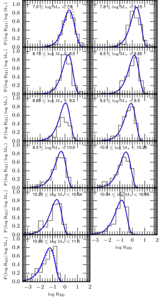
Figure 6: Distributions (PDFs) of the LTG $\rm HI$-to-stellar mass ratios in different stellar mass bins (indicated inside the panels). The gray histograms show results from the Kaplan-Meier estimator applied to the data (detections + upper limits), and the solid blue line corresponds to the best fitted number density-weighted distribution within the given mass bin (eq. 6); the constrained parameters of the mass-dependent PDF (Eq. 3) are given in Table 7. The red dotted line shows the constrained function Eq. (3) evaluated at the mass corresponding to the logarithmic center of each mass bin.

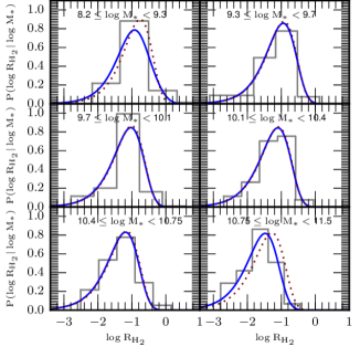
Figure 7: Same as Figure 6 but for the $\rm H_{2}$-to-stellar mass ratios.

Table 7: Best fit parameters to the full distributions

	$c$	$d$	$x_{0}$	$\log(m_{*}^{\rm tr}/\mbox{M${}_{\odot}$})$	$e$	$f$	$g$	$h$	$i$	$j$
$P(\mbox{$R_{\rm HI}$}|\mbox{$M_{*}$})$ distributions
LTG	1.11$\pm$0.35	-0.11$\pm$0.04	2.45$\pm$0.76	8.77$\pm$0.45	0.002$\pm$0.10	0.61$\pm$0.07	–	–	–	–
ETG	-0.42$\pm$0.80	-0.02$\pm$0.08	2.15$\pm$0.55	8.30$\pm$0.38	-0.43$\pm$1.10	0.52$\pm$0.09	-0.22$\pm$0.37	0.07$\pm$0.04	-1.62$\pm$1.08	-0.13$\pm$0.11
$P(\mbox{$R_{\rm H_{2}}$}|\mbox{$M_{*}$})$ distributions
LTG	0.70$\pm$1.28	-0.07$\pm$0.13	0.15$\pm$0.03	10.37$\pm$0.31	0.19$\pm$0.17	0.19$\pm$0.16	–	–	–	–
ETG	-0.52$\pm$1.19	-0.01$\pm$0.11	0.71$\pm$0.27	7.90$\pm$1.09	0.42$\pm$0.50	0.21$\pm$0.28	0.24$\pm$0.97	0.04$\pm$0.09	5.74$\pm$3.17	-0.86$\pm$0.29

• For LTGs the distributions are given by Eq. (3), while for ETGs, by Eq. (7).

Late-type galaxies.- Figures 6 and 7 present the $R_{\rm HI}$ and $R_{\rm H_{2}}$ PDFs in different $M_{*}$ bins for LTGs. Based on the bivariate $\rm HI$ and stellar mass function analysis of Lemonias et al. (2013), who used the GASS sample for (all-type) massive galaxies, we propose that the PDFs of $R_{\rm HI}$ and $R_{\rm H_{2}}$ for LTGs can be described by a Schechter (Sch) function (Eq. 3 below; $x$ denotes either $R_{\rm HI}$ or $R_{\rm H_{2}}$). By fitting this function to the $R_{\rm HI}$ data in each stellar mass bin we find that the power-law index $\alpha$ weakly depends on $M_{*}$ with most of the values being around $-0.15$ (see also Lemonias et al., 2013), while the break parameter $x^{*}$ varies with $M_{*}$. A similar behavior was found for $R_{\rm H_{2}}$ with most of the values of $\alpha$ around $-0.10$. We then perform for each case ($R_{\rm HI}$ and $R_{\rm H_{2}}$) a continuous fit across the range of stellar-mass bins rather than fits within independent bins. The general function proposed to describe the $R_{\rm HI}$ and $R_{\rm H_{2}}$ PDFs of LTGs, at a fixed $M_{*}$ and within the range $\log x\pm d\log x/2$, is:

$$P_{\rm Sch}(x|\mbox{$M_{*}$})=\frac{\phi^{*}}{\log e}\left(\frac{x}{x^{*}}\right)^{\alpha+1}\exp\left(-\frac{x}{x^{*}}\right),$$ (3)

and with the normalization condition, $\phi^{*}=1/\Gamma(1+\alpha)$, where $\Gamma$ is the complete gamma function, which guarantees that the integration over the full space in $x$ is 1. The parameters $\alpha$ and $x^{*}$ depend on $M_{*}$. We propose the following functions for these dependences:

$$\alpha(\mbox{$M_{*}$})=c+d\log\mbox{$M_{*}$},$$ (4)

and

$$x^{*}(\mbox{$M_{*}$})=\frac{x_{0}}{\left(\frac{\mbox{$M_{*}$}}{m_{\rm tr}}\right)^{e}+\left(\frac{\mbox{$M_{*}$}}{m_{\rm tr}}\right)^{f}}.$$ (5)

The parameters $c,d,x_{0},m_{\rm tr},e,$ and $f$ are constrained from a continuous fit across all the mass bins using a Markov Chain Monte Carlo method following Rodríguez-Puebla et al. (2013). Since the stellar mass bins from the data have a width, for a more precise determination, we convolve the PDF with the GSMF within a given bin. Therefore, the PDF of $x$ averaged within the bin $\Delta\mbox{$M_{*}$}=$[$\rm M_{\ast 1}$,$\rm M_{\ast 2}$] is:

$$\left\langle P_{\rm Sch}(x|\Delta\mbox{$M_{*}$})\right\rangle=\frac{\int_{\rm M_{\ast 1}}^{\rm M_{\ast 2}}P_{\rm Sch}(x|\mbox{$M_{*}$})\Phi_{late}(\mbox{$M_{*}$})d\mbox{$M_{*}$}}{\int_{\rm M_{\ast 1}}^{\rm M_{\ast 2}}\Phi_{late}(\mbox{$M_{*}$})d\mbox{$M_{*}$}},$$ (6)

where $\Phi_{late}(\mbox{$M_{*}$})$ is the GSMF for LTGs (see Section 0.6). The constrained parameters are reported in Table 7. The obtaiened mass-dependent PDFs are plotted in each one of the panels of Figures 6 and 7. The solid blue line corresponds to the number density-weighted distribution within the given mass bin (eq. 6), while the red dotted line is for the function Eq. (3) evaluated at the mass corresponding to the logarithmic center of each bin. As seen, the Kaplan-Meier PDFs obtained from the data (gray histograms) are well described by the proposed Schechter function averaged within the different mass bins (blue lines), both for $R_{\rm HI}$ and $R_{\rm H_{2}}$.

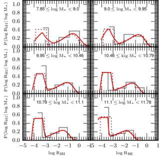
Figure 8: Distributions (PDFs) of the ETG $\rm HI$-to-stellar mass ratios in different stellar mass bins (indicated inside the panels). The gray histograms show results from the Kaplan-Meier estimator applied to the data (detections + upper limits), and the solid ted line corresponds to the best fitted number density-weighted distribution within the given mass bin (eq. 8); the constrained parameters of the mass-dependent PDF (Eq. 7) are given in Table 7. The red dotted line shows the constrained function Eq. (7) evaluated at the mass corresponding to the logarithmic center of each mass bin.

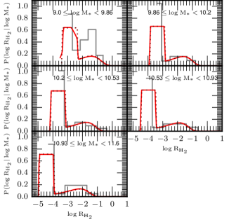
Figure 9: Same as Figure 8 but for the $\rm H_{2}$-to-stellar mass ratios.

Early-type galaxies.- We present the $R_{\rm HI}$ and $R_{\rm H_{2}}$ PDFs for ETGs in Figures 8 and 9, respectively. The distributions are very extended, implying a large scatter in the $R_{\rm H_{2}}$–$M_{*}$ correlations as discussed in subsections 0.4.2 and 0.4.3. The distributions seem to be bimodal, with a significant fraction of ETGs having gas fractions around a low limit ($\sim 10^{-4}$) and the remaining galaxies with higher gas fractions, following an asymmetrical distribution. The low limit is given by the Kaplan-Meier estimator and it is associated with the reported upper limits of non-detections. We should have in mind that when non-detections dominate, the Kaplan-Meier estimator can not provide a reliable PDF at the low end of the distribution. From a physical point of view, we know that ETGs are in general quiescent galaxies that likely exhausted their cold gas reservoirs and did not accrete more gas. However, yet small amounts of gas can be available from the winds of old/intermediate-age stars. For instance, Sun-like stars can lose $\sim 10^{-4}-10^{-5}$ of their masses in 1 Gyr; more massive stars, lose higher fractions. A fraction of the ejected material is expected to cool efficiently and ends as $\rm HI$ and/or $\rm H_{2}$ gas. On the other hand, those ETGs that have larger fractions of cold gas, could get it by radiative cooling from their hot halos or by accretion from the cosmic web, and/or by accretion from recent mergers (see for a discussion Lagos et al., 2014, and more references therein). The amount of gas acquired depends on the halo mass, the environment, the gas mass of the colliding galaxy, etc. The range of possibilities is large, hence, the scatter around the ETG $\mbox{$R_{\rm HI}$}-\mbox{$M_{*}$}$ and $R_{\rm H_{2}}$–$M_{*}$ relations are expected to be large as semi-analytic models show (Lagos et al., 2014).

To describe the PDFs seen in Figures 8 and 9, we propose a (broken) Schechter function plus a uniform distribution. The value of $R_{\rm HI}$ or $R_{\rm H_{2}}$ where the Schechter function breaks and the uniform distribution starts, $x_{2}$, seems to depend on $M_{*}$ (see Figs. 8 and 9). The lowest values where the distributions end, $x_{1}$, are not well determined by the Kaplan-Meier estimator, as mentioned above. To avoid unnecessary sophistication, we just fix $x_{1}$ as one tenth of $x_{2}$. This implies physical lowest values for $R_{\rm HI}$ and $R_{\rm H_{2}}$ of $10^{-4\div-5}$, which are plaussible according to our discussion above. The value of the Schechter parameter $\alpha$ shows a weak dependence on $M_{*}$ for both $\rm HI$ and $\rm H_{2}$. On the other hand, the fraction of galaxies between $x_{1}$ and $x_{2}$, $F$, seems to depend on $M_{*}$. For the uniform distribution, this fraction is given by $F=P(<x_{2}|\mbox{$M_{*}$})-P(<x_{1}|\mbox{$M_{*}$})=\int_{x_{1}}^{x_{2}}Cd\log x$, where $C=F/(\log x_{2}-\log x_{1})$; given our assumption of $\log x_{2}-\log x_{1}=1$ dex, then $C=F(\mbox{$M_{*}$})$. We parametrize all these dependences on $M_{*}$ and perform a continuous fit across the range of stellar-mass bins, both for the $R_{\rm HI}$ and $R_{\rm H_{2}}$ data. The general function proposed to describe the PDFs of ETGs as a function of $M_{*}$ within the range $\log x\pm d\log x/2$ is the sum of a Schechter function, $P_{\rm Sch}(x|\mbox{$M_{*}$})$, and a uniform function in $x$ but dependent on $M_{*}$, $C=F(\mbox{$M_{*}$})$:

$$F(\mbox{$M_{*}$})=g+h\log\mbox{$M_{*}$},\ \ \ \ x_{1}\leq x<x_{2}(\mbox{$M_{*}$}),$$ (7)

$$x_{2}(\mbox{$M_{*}$})=i+j\log\mbox{$M_{*}$},$$

$$P_{\rm Sch}(x|\mbox{$M_{*}$}),\ \ \ \ \ \ \ \ \ \ \ \ x\geq x_{2}(\mbox{$M_{*}$}),$$

where the parameters $x^{*}$ and $\alpha$ in $P_{\rm Sch}(x|\mbox{$M_{*}$})$ are described by Eq. (3) with the normalization condition $\phi^{*}=(1-F)/\Gamma(1+\alpha)$, and $\log x_{1}=\log x_{2}-1$. The parameters $x_{0}$, $m_{\rm tr}$, $e$, and $f$ of the broken Schechter function and the parameters $g$, $h$, $i$, and $j$ of the uniform distribution are constrained as described for LTGs above, from a continuous fit accross all the mass bins using the number density-weighted PDFs at each stellar mass bin:

$$\left\langle P_{\rm Sch}(x|\Delta\mbox{$M_{*}$})+C\right\rangle=\hskip 108.405pt$$

$$\frac{\int_{\rm M_{\ast 1}}^{\rm M_{\ast 2}}(P_{\rm Sch}(x|\mbox{$M_{*}$})+C)\cdot\Phi_{early}(\mbox{$M_{*}$})d\mbox{$M_{*}$}}{\int_{\rm M_{\ast 1}}^{\rm M_{\ast 2}}\Phi_{early}(\mbox{$M_{*}$})d\mbox{$M_{*}$}},$$ (8)

where $\Phi_{early}(\mbox{$M_{*}$})$ is the GSMF for ETGs (see Section 0.6). The constrained parameters are reported in Table 7, both for $R_{\rm HI}$ and $R_{\rm H_{2}}$. The obtained mass-dependent distribution function is plotted in each one of the panels of Figures 8 and 9 The solid red line corresponds to the number density-weighted distribution within the given mass bin (eq. 8), while the red dotted line is for the proposed broken Schechter + uniform function evaluated at the mass corresponding to the logarithmic center of each bin. As seen, the Kaplan-Meier PDFs obtained from the data (gray histograms) are reasonably well described by the proposed function (eq. 7) averaged within the different mass bins (red lines), both for $R_{\rm HI}$ and $R_{\rm H_{2}}$.

Finally, in Figures 10 and 11 we reproduce from Figure 5 the means and standard deviations obtained with the Kaplan-Meier estimator in different $M_{*}$ bins (gray dots and error bars) for LTG and ETGs, respectively, and compare them with the means and standard deviations of the general mass-dependent distributions functions given in Equations (3) and (7) and constrained with the data (black solid line and the two dotted lines surrounding it). The agreement is rather good in the log-log $R_{\rm HI}$–$M_{*}$ and $R_{\rm H_{2}}$–$M_{*}$ diagrams both for LTGs and ETGs. Black dashed lines are extrapolations of the mean and standard deviation inferences from the distributions mentioned above, assuming they are the same as in the last mass bin with available gas observations. We also plot in these Figures the respective mean double power-law relations determined in subsections 0.4.2 and 0.4.3 (dashed blue or red lines, for LTGs and ETGs respectively; dotted blue or red lines are extrapolations.).

In conclusion, the $R_{\rm HI}$ and $R_{\rm H_{2}}$ distributions as a function of $M_{*}$ described by Equations (3) and (7) (with the parameters given in Table 7) for LTGs and ETGs, respectively, are fully consistent with the corresponding $R_{\rm HI}$–$M_{*}$ and $R_{\rm H_{2}}$–$M_{*}$ correlations determined in subsections 0.4.2 and 0.4.3. Therefore, Equations (3) and (7) provide a consistent description of the $\rm HI$- and $\rm H_{2}$-to-stellar mass relations and their scatter distributions, for LTGs and ETGs, respectively.

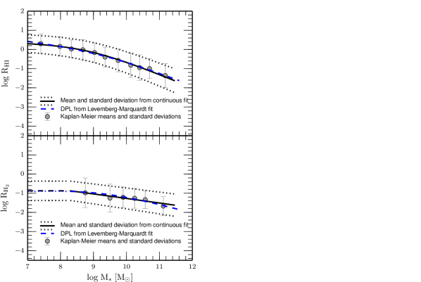
Figure 10: Mean and standard deviation as a function of stellar mass (solid and dotted black lines) from the distributions of $R_{\rm HI}$ (upper panel) and $R_{\rm H_{2}}$ (lower panel) for LTGs as given by Eq. (3) (see Table 7 for the constrained parameters). When the data are insufficient at low masses, the distributions are assumed the same as in the last mass bin (dashed black lines). The gray dots with error bars are the mean and standard deviation obtained with the Kaplan-Meier estimator applied to the data (detections + upper limits) in different mass bins, as shown in Figure 5. The double-power law fits to these data as reported in Section 4 are reproduced with the blue dashed lines (the blue dotted lines are extrapolations of these fits).

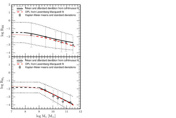
Figure 11: Same as in Figure 10 but for ETGs.

0.6 Consistency of the gas-to-stellar mass correlations with the observed galaxy gas mass functions

The $\rm HI$- and $\rm H_{2}$-to-stellar mass relations can be used to map the observed GSMF into the $\rm HI$ and $\rm H_{2}$  mass functions (G$\rm HI$MF and G$\rm H_{2}$MF, respectively). This way, we can check whether the correlations we have inferred from observations in subsectiona 0.4.2 and 0.4.3 are consistent or not with the G$\rm HI$MF and G$\rm H_{2}$MF obtained from $\rm HI$ and CO ($\rm H_{2}$) surveys, respectively. In order to carry out this check of consistency, we need a GSMF, on one hand, defined in a large enough volume as to include massive galaxies and to minimize cosmic variance, and on the other hand, complete down to very low masses. As a first approximation to obtain this GSMF, we follow here a procedure similar as in Kravtsov et al. (2014, see their Appendix A). We use the combination of two GSMFs: Bernardi et al. (2013) for the large SDSS volume (complete from $\mbox{$M_{*}$}\sim 10^{9}$ M_⊙), and Baldry et al. (2012) for a local small volume but nearly complete down to $\mbox{$M_{*}$}\sim 10^{7}$ M_⊙ (GAMA). In Appendix .14 we describe how we apply some corrections and homogenize both samples to obtain an uniform GSMF from $\mbox{$M_{*}$}\sim 10^{7}$ to $\sim 10^{12}$ M_⊙.

Figure 12 presents our combined GSMF (solid line) and some GSMFs reported in the literature: the two used by us (see above), and those from Wright et al. (2017), Papastergis et al. (2012), and Baldry et al. (2008) in small but deep volumes, and D’Souza et al. (2015) in a large volume. We plot both the original data from Bernardi et al. (2013) (pink symbols) and after dismissing $M_{*}$ by 0.12 dex (blue symbols) to homogenize the stellar masses to the BC03 population synthesis model (see Appendix .14). There is very good agreement between our combined GSMF and the recent GSMF reported in Wright et al. (2017) for the GAMA data.

Since the GSMF will be used as an interface for constructing the $\rm HI$ and $\rm H_{2}$ mass functions, it is implicit the assumption that each galaxy with a given stellar mass has its respective $\rm HI$ and $\rm H_{2}$ content. Hence, the gas mass functions presented below exclude the possibility of galaxies with gas content but not stars, and are equivalent to gas mass functions constructed from optically-selected samples (as in e.g., Baldry et al., 2008; Papastergis et al., 2012). In any case, it seems that the probability of finding only-gas galaxies is very low (Haynes et al., 2011).

Figure 12: Our GSMF obtained from the combination of three observational GSMFs following Kravtsov et al. (2014) (thick solid line): one from the large SDSS DR7 volume but complete only down to $\sim 10^{9}$ M_⊙ (Bernardi et al., 2013, pink open circles with error bars; the orange open circles with error bars are after correcting $M_{*}$ by 0.12 dex, see text), and two complete down to lower masses but in a very local volume (Wright et al. (2017), Papastergis et al., 2012 and Baldry et al., 2012). We also plot for comparison, the GSMFs reported in Baldry et al. (2008) and D’Souza et al. (2015). The lower panel shows the fraction of ETGs as a function of mass inferred by Moffett et al. (2016), using GAMA galaxies and their visual morphological classification.

We generate a volume complete mock galaxy catalog that samples the empirical GSMF presented above, and that takes into account the empirical volume-complete fraction of ETGs, $f_{\rm early}$, as a function of stellar mass (the complement is the fraction of LTGs, $f_{\rm late}=1-f_{\rm early}$). The catalog is constructed as follows:

1. A minimum galaxy stellar mass $M_{\rm*,min}$ is set ($=10^{7}$ M_⊙). From this minimum we generate a population of $5\times 10^{6}$ galaxies that samples the GSMF presented above.

2. Each mock galaxy is assigned either as LTG or ETG. For this, we use the results reported in Moffett et al. (2016), who visually classified galaxies from the GAMA survey. They consider ETGs those classified as Ellipticals and S0-Sa galaxies. The $f_{\rm early}$ fraction as a function of $M_{*}$ is calculated as $\Phi_{\rm early}(\mbox{$M_{*}$})/\Phi_{\rm all}(\mbox{$M_{*}$})$, with $\Phi_{\rm early}(\mbox{$M_{*}$})=\Phi_{\rm Ell}(\mbox{$M_{*}$})+\Phi_{\rm S0-Sa}(\mbox{$M_{*}$})$, using the fits to the respective GSMFs reported in Moffett et al. (2016).

3. For each galaxy, $R_{\rm HI}$ is assigned randomly from the conditional probability distribution $P_{j}(\mbox{$R_{\rm HI}$}|\mbox{$M_{*}$})$ that a galaxy of mass $M_{*}$ and type $j=$LTG or ETG lies in the $\mbox{$R_{\rm HI}$}\pm d\mbox{$R_{\rm HI}$}/2$ bin. Then, $M_{HI}$=$R_{\rm HI}$$\times$$M_{*}$. The probability distributions for LTGs and ETGs are given by the mass-dependent PDFs presented in Equations (3) and (7), respectively (their parameters are given in Table 7).

4. The same procedure as in the previous item is applied to assign $M_{H_{2}}$=$R_{\rm H_{2}}$$\times$$M_{*}$, by using for the $P_{j}(\mbox{$M_{H_{2}}$}|\mbox{$M_{*}$})$ probability distributions the corresponding mass-dependent PDFs for LTGs and ETGs presented in Equations (3) and (7), respectively (their parameters are given in Table 7).

Our mock galaxy catalog is a volume-complete sample of $5\times 10^{6}$ galaxies above $\mbox{$M_{*}$}=10^{7}$ M_⊙, corresponding to a co-moving volume of $5.08\times 10^{7}$ Mpc³. Since the $\rm HI$ and $\rm H_{2}$ mass functions are constructed from the GSMF, its mass limit $M_{\rm*,min}$ will propagate in different ways to these mass functions. The co-moving volume in our mock galaxy catalog is big enough as to avoid significant effects from Poisson noise. This noise affects specially the counts of massive galaxies, which are the less abundant objects.

Figure 13: Panel (a): Total GSMF from the mock catalog that reproduces the empirical GSMF of Fig. 12 (solid line). The gray shadow represents the Poisson errors (except for large masses, these errors are thinner than the line thickness). The GSMF from the mock catalog samples very well the empirical GSMF used as input. The blue/red dotted lines and shadows correspond to the LTG/ETG mass function components, using the empirical ETG fraction as a function of $M_{*}$ shown in Fig. 12. Panel (b): Same as in panel (a) but for atomic gas, using the mean $R_{\rm HI}$–$M_{*}$ relation and its scatter distribution as given in section 0.5. Several observational G$\rm HI$MF’s from blind $\rm HI$ samples, and the ETG G$\rm HI$MF from ATLAS^3D and HIPASS surveys are reproduced (see labels inside the panel). Panel (c): Same as in panel (a) but for molecular gas. The G$\rm H_{2}$MF calculated from the Keres et al. (2003) L_CO function is reproduced. The dotted purple line is the total G$\rm H_{2}$MF from the mock catalog when using a $R_{\rm H_{2}}$–$M_{*}$  correlation obtained from our compilation but assuming that $\alpha_{\rm CO}$=$\alpha_{\rm CO,MW}$=const., as done in Keres et al. (2003).

0.6.1 The mock galaxy mass functions

Stellar mass function

The mock GSMF is plotted in panel (a) of Fig. 13 along with the Poisson errors given by the thickness of the gray line; except for the highest masses, the Poisson errors are actually thinner than the line. The mock GSMF is an excellent realization of the empirical GSMF (compare it with Fig. 12). We also plot the corresponding contributions to the mock GSMF from the LTG and ETG populations (blue and red dashed lines). As expected, LTGs dominate at low stellar masses and ETGs dominate at high stellar masses. The contribution of both populations is equal ($f_{\rm early}=f_{\rm late}=0.5$) at $\mbox{$M_{*}$}^{\rm cross}=10^{10.20}$ M_⊙  (recall that the fraction $f_{\rm early}$ used here comes from Moffett et al. (2016), who included Sa galaxies as ETGs; if consider Sa galaxies as LTGs, then $\mbox{$M_{*}$}^{\rm cross}$ would likely be higher). In order to predict accurate gas and baryonic mass functions, the present analysis will be further refined in Rodriguez-Puebla et al. (in prep.), where several sources of systematic uncertainty in the GSMF measurement and in the definition of the LTG/ETG fractions will be taken into account. Our aim here is only to test whether the empirical correlations derived in Section 0.4 are roughly consistent or not with the total $\rm HI$ and $\rm H_{2}$ empirical mass functions.

$\rm HI$ mass function

In panel (b) of Fig. 13, we plot the predicted G$\rm HI$MF from our mock galaxy catalog using the mean (LTG+ETG) $R_{\rm HI}$–$M_{*}$ relations and their scatter distributions as given in section 0.5 (black line, the gray shadow shows the Poisson errors). For comparison, we plot also the $\rm HI$ mass functions estimated from the blind $\rm HI$ surveys ALFALFA (Martin et al., 2010; Papastergis et al., 2012, for both their $\rm HI$- and optically-selected samples; and the latest results from Jones et al., 2018) and HIPASS (Zwaan et al., 2005). At masses larger than $\mbox{$M_{HI}$}\sim 3\times 10^{10}$ M_⊙, our G$\rm HI$MF is in vey good agreement with those from the ALFALFA survey but significantly above than the HIPASS one. Martin et al. (2010) argue that the larger volume of ALFALFA survey compared to the HIPASS one, makes ALFALFA more likely to sample the mass function at the highest masses, where objects are very rare. The volume of our mock catalog is even larger than the ALFALFA one. At intermediate masses, $9\lesssim\log$($M_{HI}$/M_⊙)$\lesssim 10.5$, our G$\rm HI$MF is in reasonable agreement with the observed mass functions but it has in general a slightly less curved shape than these functions. At low masses, $\log$($M_{HI}$/M_⊙)$\lesssim 8$, the observed G$\rm HI$MF’s flatten more than our predicted mass function. It could be that the blind surveys start to be incomplete due to sensitivity limits in the radio observations. Note that Papastergis et al. (2012) imposed additional optical requirements to their $\rm HI$ blind sample (see their Section 2.1), which make flatter the low-mass slope. Regarding the optically-selected sample of Papastergis et al. (2012), since it is constructed from a GSMF that starts to be incomplete below $\log$($M_{*}$/M_⊙)$\sim 8$ (see Fig. 12), one expects incompleteness in the G$\rm HI$MF starting at a larger mass in $\rm HI$. Since our G$\rm HI$MF is mapped from a volume-complete GSMF from $M_{\rm*,min}\approx 10^{7}$ M_⊙, “incompleteness” in $M_{HI}$ is expected to start from the $\rm HI$ masses corresponding to $M_{\rm*,min}\times P(\mbox{$R_{\rm HI}$}|M_{\rm*,min})$, where the latter is the scatter around the $R_{\rm HI}$–$M_{*}$ relation. This shows that our G$\rm HI$MF can be considered complete from $\log$($M_{HI}$/M_⊙)$\approx 8$. The slope of the G$\rm HI$MF around this mass is $-1.52$, steeper than the slope at the low-mass end of the corresponding GSMF ($\alpha=-1.47$).

In Fig. 13 are also plotted the LTG and ETG components of the G$\rm HI$MF as obtained from our mock catalog. The G$\rm HI$MF is totally dominated by the contribution of LTGs. Our ETG G$\rm HI$MF is compared with the ones obtained from observations by using the ATLAS^3D and HIPASS surveys as reported in Lagos et al. (2014).

$\rm H_{2}$ mass function

In panel (c) of Fig. 13, we plot the predicted G$\rm H_{2}$MF from our mock galaxy catalog using the mean (LTG+ETG) $R_{\rm H_{2}}$–$M_{*}$ relations and their scatter distributions as given in section 0.5 (black line, the gray shadow shows the Poisson errors). We compute the $\rm H_{2}$ mass function from the CO luminosity function derived by Keres et al. (2003), who used the small and incomplete FCRAO CO survey (Young et al., 1995) and combined it with the volume-complete FIR survey. We adopt the MW $\rm H_{2}$-to-$\rm CO$ conversion factor and correct their $h$ parameter to 0.7. Unfortunately, this derivation is highly uncertain since is based on a empirical correlation between the 60$\mu$m and CO luminosities, and the selection effects in both used surveys introduce several biases. The obtained G$\rm H_{2}$MF is plotted in Fig. 13. Our G$\rm H_{2}$MF decreases faster than the one by Keres et al. (2003) at high masses, roughly agrees with it at intermediate masses, and for masses below $\log$($M_{H_{2}}$/M_⊙)$\sim 8.5$, our mass function is steeper. The reason for this latter difference seems to be the mass-dependent $\rm CO\mbox{-to-}H_{2}$ conversion factor introduced by us (see Appendix .11). This factor increases as $M_{*}$ is smaller while in the case of Keres et al. (2003) it is constant. We recalculate the G$\rm H_{2}$MF by using in the conversion from $L_{\rm CO}$ to $M_{H_{2}}$ a constant $\rm CO\mbox{-to-}H_{2}$ factor equal to the MW value, and plot it with the purple dotted line; the mass function at the low-mass side is now in good agreement with that of Keres et al. (2003).

In Fig. 13 are also plotted the LTG and ETG components of the G$\rm H_{2}$MF as obtained from our mock catalog. The G$\rm H_{2}$MF is totally dominated by the contribution of LTGs. Our ETG G$\rm H_{2}$MF is compared with the one obtained from observations by using the ATLAS^3D survey as reported in Lagos et al. (2014).

0.7 Discussion

0.7.1 The $\rm H_{2}$-to-$\rm HI$ mass ratio

The global $\rm H_{2}$-to-$\rm HI$ mass ratio of a galaxy characterizes its global efficiency of converting atomic into molecular hydrogen. This efficiency is tightly related to the efficiency of large-scale SF in the galaxy (see e.g., Leroy et al., 2008). From the empirical correlations inferred in Section 0.4, we can calculate $M_{H_{2}}$/$M_{HI}$ as a function of $M_{*}$ for both the LTG and ETG populations. We do this by using our double power-law fits to the data. Left panel of Fig. 14 presents the obtained $M_{H_{2}}$/$M_{HI}$–$M_{*}$ relations and their $1\sigma$ scatter calculated by propagating the dispersions in the assumption of null covariance. In this sense, the plotted scatter are upper limits, since there is evidence of some (weak) correlation between the $\rm HI$ and $\rm H_{2}$ content of galaxies, in particular among those deficient in $\rm HI$ and $\rm H_{2}$ (Boselli et al., 2014c). We can plot the same correlations from the mock catalog presented in Section 0.6, which samples the observed GSMF, the LTG and ETG fractions as a function of $M_{*}$, and the empirical correlations inferred by us. The middle panels of Fig. 14 present what we measure from the mock catalog for LTG (blue), ETG (red), and all galaxies (gray). The lines are the logarithmic means in small mass bins and the shaded regions are the corresponding standard deviations. At low masses, LTGs dominate, so the correlation of all galaxies is practically the one of LTGs. At high masses, ETGs become more important.

Figure 14: Left panels: Molecular-to-atomic mass ratio, $M_{H_{2}}$/$M_{HI}$, for LTGs (upper panel) and ETGs (lower panel) inferred from our double power-law fits to the $R_{\rm HI}$-$M_{*}$ and $R_{\rm H_{2}}$-$M_{*}$ correlations. The shaded areas are the 1$\sigma$ scatter obtained by error propagation of the scatter around the $R_{\rm HI}$-$M_{*}$ relations. Middle panels: Same as in left panels but from our mock catalog generated to sample the empirical GSMF, volume-complete ETG/LTG fractions as a function of mass, and $R_{\rm HI}$–$M_{*}$ and $R_{\rm H_{2}}$–$M_{*}$ correlations. The dotted line surrounded by the gray area are the total $M_{H_{2}}$/$M_{HI}$ ratio and 1$\sigma$ scatter as a function of stellar mass. Right panels: Molecular-to-atomic mass ratio as a function of the cold gas mass, $M_{\rm gas}$, from the mock catalog for LTGs (upper panel) and ETGs (lower panel). We plot available detected and undetected cold gas observational data as gray unfilled circles and downward arrows respectively.

According to Fig. 14, the molecular-to-atomic mass ratio of LTGs increases with $M_{*}$, albeit with a large scatter. On average, $M_{H_{2}}$/$M_{HI}$ increases from $\approx 0.1$ to $\approx 0.8$ for masses ranking from $\mbox{$M_{*}$}=10^{8}$ M_⊙ to $3\times 10^{11}$ M_⊙. Given that the surface density of LTGs correlates significantly with $M_{*}$, one can expect this dependence of $M_{H_{2}}$/$M_{HI}$ on $M_{*}$ at least from two arguments: 1) Disk instabilities, which drive the formation of molecular clouds (e.g., the Toomre criterion Toomre, 1964), are more probable to occur as the disk surface density is higher. 2) The $\rm H_{2}$-to-$\rm HI$ mass ratio in galaxies has been shown to be directly related to the hydrostatic gas pressure (Blitz & Rosolowsky, 2006; Krumholz et al., 2009), and this pressure depends on the (gas and stellar) surface density (Elmegreen, 1989). In fact, the physics of $\rm H_{2}$ condensation from $\rm HI$ is very complex and it is expected to be driven by local parameters of the ISM (see e.g., Blitz & Rosolowsky, 2006; Krumholz et al., 2009; Obreschkow & Rawlings, 2009). Therefore, the dependence of the $\rm H_{2}$-to-$\rm HI$ mass ratio on $M_{*}$ should be understood as consequence of the correlations of these parameters (their mean values along the galaxy) with $M_{*}$, introducing this actually a large scatter in the dependence of $M_{H_{2}}$/$M_{HI}$ on $M_{*}$. Indeed, several authors have shown that $M_{H_{2}}$/$M_{HI}$ correlates better with the mean gas-phase metallicity or mean stellar surface density than with $M_{*}$ (e.g., Saintonge et al., 2011; Boselli et al., 2014a).

For ETGs, the trend of the $\rm H_{2}$-to-$\rm HI$ mass ratio is inverse to the one of LTGs and with a very large scatter. The ETGs more massive than $\sim 10^{11}$ M_⊙ have mean ratios around $0.15$ and a 1-$\sigma$ scatter of $\sim\pm 1$ dex; for intermediate masses, this ratio increases on average, and for ETGs with masses $\mbox{$M_{*}$}\sim 10^{9}$ M_⊙, which are actually very rare, their mean $\rm H_{2}$-to-$\rm HI$ mass ratios are $\sim 1$ with the same scatter of $\sim\pm 1$ dex. Even though the gas fraction in ETGs is much smaller than in LTGs at all masses (see Fig. 5), the former are also typically more compact than the latter, resulting probably on average in similar or higher gas pressures, and consequently a similar or even higher $M_{H_{2}}$/$M_{HI}$ ratios, specially at masses lower than $\mbox{$M_{*}$}\approx 10^{10}$ M_⊙. In fact, given the large scatter in $M_{H_{2}}$/$M_{HI}$ for ETGs, this ratio depends likely on many other internal and external (mergers, environment, etc.) factors that do not correlate significantly with $M_{*}$.

Regarding $M_{H_{2}}$/$M_{HI}$ vs. $M_{\rm gas}$, for LTGs, which for $\mbox{$M_{*}$}>10^{7}$ M_⊙ have mostly gas masses $>10^{8}$ M_⊙, there is not any significant dependence, while for ETGs, which are almost inexistent with $\mbox{$M_{\rm gas}$}\gtrsim 10^{9}$ M_⊙, $M_{H_{2}}$/$M_{HI}$ is larger on average for lower values of $M_{\rm gas}$. This can be seen in the right panel of Fig. 14, where the mock catalog has been used. Basically, for a given $M_{\rm gas}$, in the mass range $\mbox{$M_{\rm gas}$}\sim 10^{7}-10^{9}$ M_⊙), ETGs have typically larger $\rm H_{2}$-to-$\rm HI$ mass ratios than LTGs. In combination, the $\rm H_{2}$-to-$\rm HI$ ratio appears to be larger for lower values of $M_{\rm gas}$. Such a dependence has been reported by Obreschkow & Rawlings (2009) for their compiled sample of galaxies, and predicted by these authors from a physical model.

The dependences of the $\rm H_{2}$-to-$\rm HI$ mass ratio on $M_{*}$, $M_{\rm gas}$, and morphological type discussed above are in qualitative agreement with several previous observational works, which actually are part of our compilation (Leroy et al., 2008; Obreschkow & Rawlings, 2009; Saintonge et al., 2011; Boselli et al., 2014a; Bothwell et al., 2014). However, our results extend to a larger mass range and separate explicitly the two main populations of galaxies.

0.7.2 The role of environment

There are several pieces of evidence that the atomic gas fraction of galaxies is lower in higher-density environments (e.g., Haynes & Giovanelli, 1984; Gavazzi et al., 2005; Cortese et al., 2011; Catinella et al., 2013; Boselli et al., 2014c). The fact that the ETG population has lower $\rm HI$ gas fractions than the LTG one (Section 0.4), being the former commonly found in higher-density environments, agrees with the mentioned trends with environment. Thus, due to the morphology-density relation, our determinations of the $R_{\rm HI}$–$M_{*}$ (as well as $R_{\rm H_{2}}$–$M_{*}$ and $R_{\rm gas}$–$M_{*}$) correlations for the LTG and ETG populations, account partially for the dependence of these correlations on environment. Moreover, for the very isolated LTGs and for the subsample of LTGs in the Virgo cluster central regions, we confirm higher and lower $\rm HI$-to-stellar mass ratios than the average of the overall LTG sample, respectively (see subsection 0.3.1). However, this systematical difference with the environment is within the $1\sigma$ scatter of the $R_{\rm HI}$–$M_{*}$ correlation of LTGs (see Fig. 3). Instead, in the case of ETGs, the isolated galaxies have much larger $R_{\rm HI}$ values than the means of all ETGs, above the $1\sigma$ scatter; isolated ETGs are almost as $\rm HI$ gas rich as the mean of LTGs.

For molecular gas fraction, the observational results are controversial in the literature. Recent studies seem to incline the controversy to the fact that galaxies in clusters are actually $\rm H_{2}$–deficient with respect to similar galaxies in the field, however, the deficiencies are smaller than in the case of $\rm HI$ (Boselli et al., 2014c, and more references therein). Here, for isolated and Virgo-center LTGs, we do not see any systematical segregation of $R_{\rm H_{2}}$ from the rest of our compiled LTGs (Fig. 4), but in the case of ETGs, the isolated galaxies have on average larger values of $R_{\rm H_{2}}$.

In summary, the results from our compilation point out that the $\rm HI$ content of LTGs has a (weak) dependence on environment, mainly due to the fact that at high densities LTGs are $\rm HI$ deficient. Instead, the $\rm H_{2}$ content of LTGs seems not to change on average with the environment. In the case of ETGs, those very isolated are significantly more gas rich (both in $\rm HI$ and $\rm H_{2}$) than the average among ETGs at a given mass.

An important aspect related to the environment is whether a galaxy is central or satellite. The local environmental effects once a galaxy becomes a satellite inside a halo (ram pressure and viscous stripping, starvation, harassment, tidal interactions) work in the direction of lowering the gas content of the galaxy, likely more as more massive is the halo (Boselli & Gavazzi, 2006; Brown et al., 2017). Part of the scatter in the gas-to-stellar mass correlations are probably due to the external processes produced by these local-environment mechanisms. A result in this direction has been recently shown for the $R_{\rm HI}$–$M_{*}$ correlation by Brown et al. (2017). These authors have found that the $\rm HI$ content of satellite galaxies in more massive halos have, on average, lower $\rm HI$-to-stellar mass ratios at fixed stellar mass and specific SFR. According to their analysis, the systematic environmental suppression of $\rm HI$ content at both fixed stellar mass and fixed specific SFR in satellite galaxies begins in halo masses typical of the group regime ($>10^{13}$ M_⊙), and fast-acting mechanisms such as ram-pressure stripping are suggested to explain their results. In a future work, we will attempt to characterize the central/satellite nature of our compiled galaxies, as well as to calculate a proxy to their halo masses, in order to study this question.

0.7.3 Comparisons with previous works

In Fig. 15 we compare our results with those of previous works. When necessary, the data are corrected to a Chabrier (2003) IMF. Most of the previous determinations of the $\rm HI$- and $\rm H_{2}$-to-stellar mass correlations are not explicitly separated into the two main galaxy populations as done here, and in several cases non detections are assumed to have the values of the upper limits or are not taken into account at all.

In the upper panel, our empirical $R_{\rm HI}$–$M_{*}$ correlations for LTGs and ETGs are plotted along with the linear relations given by Stewart et al. (2009) (cyan line, the dashed lines show the $1\sigma$ scatter) and Papastergis et al. (2012) (gray line). The former authors used mainly the observational data presented in McGaugh (2005) for disk-dominated galaxies, and the latter authors used samples from Swaters & Balcells (2002), Garnett (2002), Noordermeer et al. (2005), and Zhang et al. (2009), which refer mostly to late-type galaxies. Their fits are slightly above the mean of our LTG $R_{\rm HI}$–$M_{*}$ correlation. This is likely because they ignore non-detections. We also plot the logarithmic average values in mass bins reported by Catinella et al. (2013) for GASS (green open circles). Since ETGs progressively dominate in number as the mass increase, our total (density-weighted) $R_{\rm HI}$–$M_{*}$ correlation would fall below the one by Catinella et al. (2013), specially at the highest masses. Note that for the data plotted from Catinella et al. (2013), the $\rm HI$ masses of non-detections were set equal to their upper limits. Therefore, the plotted averages are biased to high values of $R_{\rm HI}$, specially for ETGs which are dominated by non-detections. On the other hand, recall that we have corrected by distance the upper limits of GASS to make them compatible with those of the closer ATLAS^3D survey.

More recently, Brown et al. (2015) have used the $\rm HI$ spectral stacking technique for a volume-limited, stellar mass selected sample from the intersection of SDSS DR7, ALFALFA, and $GALEX$ surveys. With this technique the stacked signal of co-added raw spectra of detected and non-detected galaxies (about 80% of the ALFALFA selected sample) is converted into a (lineal) average $\rm HI$ mass. The authors have excluded from their analysis $\rm HI$-deficient galaxies –typically found within clusters– because of their significant offset to lower gas content. The black dots connected by a dotted line show the logarithm of the average $R_{\rm HI}$ values reported at different stellar mass bins in Brown et al. (2015). Since $\rm HI$-deficient galaxies –which typically are ETGs– were excluded, then the Brown et al. (2015) correlation should be compared with our correlation for LTGs. Note that with the stacking technique is not possible to obtain the population scatter in $R_{\rm HI}$ because the reported mean values come from stacked spectra instead from averaging individual values of detections and non detections. However, the stacking can be applied to subsets of galaxies, for example, selected by color. Brown et al. (2015) have divided their sample into three groups by their NUV$-r$ colors: [1,3), [3,5), and [5,8]. The average $R_{\rm HI}$ values at different masses corresponding to the bluest and reddest groups are reproduced in Fig. 15 with the blue and red symbols, respectively. Note that the logarithmic mean is lower than the logarithm of the mean. For a lognormal distribution, $\langle\log x\rangle=\log\langle x\rangle-0.5\times\sigma^{2}_{\log x}\ln 10$ (see e.g., Rodríguez-Puebla et al., 2017). Then, for the typical scatter of 0.44 dex corresponding to LTGs, the logarithm of the stacked values of $R_{\rm HI}$ should be lowered by $\approx 0.2$ dex to compare formally with our reported values of logarithmic means; this is shown with a black arrow in Fig. 15. If the reddest galaxies in the Brown et al. (2015) stacked sample are associated with ETGs (which is true only partially), then for them the correction to a logarithmic mean is of $\approx 1$ dex, shown with a red arrow.

Figure 15: Upper panel: Our empirical $\rm HI$-to-stellar mass correlations for LTGs and ETGs (blue and red shaded areas, respectively) compared with some previous determinations (see labels inside the panel and details of each determination in the text). These previous determinations are for compilations typically biased to late-type, blue galaxies, and/or do not take into account non detections. The blue and red arrows correspond to estimates of the difference between the logarithm of the mean (the stacking technique provides the equivalent of the mean value) and the logarithmic mean (our determinations are for this case) for standard deviations of 0.52 and 0.99 dex, respectively (see text for more details). Lower panel: Our empirical molecular $\rm H_{2}$-to-stellar mass correlations for LTGs and ETGs (blue and red shaded areas, respectively) compared with very rough previous determinations not separated into LTGs and ETGs (see labels inside the panel and details of each determination in the text).

Finally, recently van Driel et al. (2016) reported the results from $\rm HI$ observations at the Nancay Radio Telescope (NRT) of 2839 galaxies selected evenly from SDSS. The authors present a Buckley-James linear regression to their data (long-dashed green line in Fig. 15), taking into account this way upper limits for non-detections (though their upper limits are quite high given the low sensitivity of NRT). Their fit is for all the sample, that is, they do not separate into LTG/ETG or blue/red groups. In a subsequent paper (Butcher et al., 2016), the authors obtained $\sim 4$ times more sensitive follow-up $\rm HI$ observations at Arecibo for a fraction of the galaxies that were either not detected or marginally detected; 80% of them were detected with $\rm HI$ masses $\sim 0.5$ dex lower than the upper limits in van Driel et al. (2016), and the rest, mostly luminous red galaxies, were not detected. If this trend is representative of the rest of the NRT undetected galaxies, Butcher et al. (2016) expect the fit plotted in Fig. 15 to be offset toward lower $R_{\rm HI}$ values by about 0.17 dex and even more at the highest masses. This fit is in between a density-weighted fit to our two correlations when taking into account that at high masses the fraction of ETG/red galaxies increases and at low masses LTG/blue galaxies dominate at all.

The lower panel of Fig. 15 is similar to the upper panel but for the $R_{\rm H_{2}}$–$M_{*}$ correlations. In the case of the molecular gas content, in the literature there are only a few attempts to determine the relation between $M_{H_{2}}$ and $M_{*}$. In fact, those works that report approximate correlations are included in our compilation: Saintonge et al. (2011) for COLD GASS, and Boselli et al. (2014a) for HRS. The former authors report a linear regression to their binned data assuming $\rm H_{2}$ masses for non-detection set equal to their upper limits. The latter authors present a bisector fit using only detected, late-type gas-rich galaxies. Therefore, in both cases the reported relations are clearly biased to LTGs and to the side of high $R_{\rm H_{2}}$ values.

The differences we find between our correlations and those plotted in Fig. 15, as discussed above, can be understood on the basis of the different limitations that present each one of the previous works. Having in mind these limitations in each concrete case, we can conclude that the correlations presented here are in rough agreement with previous ones but with respect to them (i) extend the correlations to a larger mass range, (ii) separate explicitly galaxies into their two main populations, and (iii) take into account adequately the non detections.

0.8 Summary and Conclusions

The fraction of stars and atomic and molecular gas in local galaxies is the result of complex astrophysical processes across their evolution. Thus, the observational determination of how these fractions vary as a function of mass provides key information on galaxy evolution at different scales. Before the new generation of radio telescopes, which will bring extragalactic gas studies more in line with optical surveys, the main way to get this kind of information is from studies based on radio follow-up observations of (small) optically-selected galaxy samples. In this work, we have compiled and homogenized from the literature samples with information on $M_{*}$ and $M_{HI}$ and/or $M_{H_{2}}$ for galaxies that can be identified belonging to two main operational (in a statistical sense) groups: the LTG and ETG populations. For estimating $M_{H_{2}}$ from CO observations, we have introduced a mass-dependent $\rm CO\mbox{-to-}H_{2}$ conversion factor in agreement with studies that show that this factor is not constant and depends on metallicity (hence, statistically on mass). Results using a constant $\rm CO\mbox{-to-}H_{2}$ factor were also presented. Figures 1 and 2 summarize our compilation in the $R_{\rm HI}$ vs. $M_{*}$ and $R_{\rm H_{2}}$ vs. $M_{*}$ logarithmic diagrams.

Previous to infer the correlations, we have tested how much each one of the compiled samples deviate from the rest and classified them into three categories: (1) samples complete in limited volumes (or selected from them) without selection effects that could affect the calibration of the correlations (Golden), (2) samples that are not complete but are representative of the average galaxy population, without obvious selection effects (Silver), and (3) samples selected by environment (Bronze). We showed that most of the samples, after our homogenization, are suitable to infer the $R_{\rm HI}$–$M_{*}$ and $R_{\rm H_{2}}$–$M_{*}$ correlations, except those from the Bronze category in the case of ETGs. These galaxies in extreme environments show significant deviations from the mean trends, and then are not taken into account in our determinations. From the combination of all the chosen samples, we have calculated the mean, standard deviation, and percentiles of the logarithms of the $R_{\rm HI}$ and $R_{\rm H_{2}}$ mass ratios in several stellar mass bins, taking into account non-detected galaxies and their reported upper limits, which are a non-negligible fraction of the data, specially for the ETG population. The accounting of non-detected galaxies and their homogenization among different samples are relevant for determining the gas-to-stellar mass correlations of ETGs.

The mean logarithmic values in mass bins, $\langle\log\mbox{$R_{\rm HI}$}\rangle$ and $\langle\log\mbox{$R_{\rm H_{2}}$}\rangle$, with the corresponding (intrinsic) standard deviation calculated by means of the Kaplan-Meier estimator were fitted to the logarithm of single and double power-law functions (Eq. 1). The parameters of the best fits to these functions, both for LTGs and ETGs, are reported in Tables 5 and 6, respectively. We highlight the following results from our analysis:

$\bullet$ The $R_{\rm HI}$–$M_{*}$ and $R_{\rm H_{2}}$–$M_{*}$ correlations for the LTG and ETG populations, can be described roughly equally well by a single or double power law at masses larger than $\log$($M_{*}$/M_⊙)$\gtrsim 9$. For smaller masses, we see some hints of a flattening in these correlations. LTGs have significantly higher $\rm HI$ and $\rm H_{2}$ gas fractions than ETGs, the differences increasing at the high- and low-stellar mass ends. For the ETG population, the scatter of the $R_{\rm HI}$–$M_{*}$ and $R_{\rm H_{2}}$–$M_{*}$ correlations are much larger than for the LTG one.

$\bullet$ Combining the $R_{\rm HI}$–$M_{*}$ and $R_{\rm H_{2}}$–$M_{*}$ correlations and propagating errors, we calculated the cold gas ($M_{\rm gas}$=1.4($M_{HI}$+ $M_{H_{2}}$))-to-stellar mass correlations of the LTG and ETG populations. For the former, $R_{\rm gas}$ is around 4 on average at $\mbox{$M_{*}$}=10^{7}$ M_⊙ and $\approx 1$ at $\mbox{$M_{*}$}=1.60\times 10^{9}$ M_⊙. At larger masses, $R_{\rm gas}$ continues decreasing sifnificantly. For the ETG population, $R_{\rm gas}$ on average is smaller than 1 even for the smallest galaxies. Galaxies as massive as $\mbox{$M_{*}$}=10^{11}$ M_⊙ have on average $R_{\rm gas}$ ratios smaller than $2.5\times 10^{-3}$. The intrinsic standard deviation of the $R_{\rm gas}$–$M_{*}$ correlation of the LTG population is $\approx 0.44$ dex while for the ETG one is larger, around 0.68 dex.

$\bullet$ The $\rm H_{2}$-to-$\rm HI$ mass ratio implied by our correlations is such that for LTGs, increases on average with $M_{*}$, from $\approx 0.1$ to $0.8$ for masses ranking from $\mbox{$M_{*}$}=10^{8}$ M_⊙ to $3\times 10^{11}$ M_⊙. For ETGs, the trend is the opposite but with large scatter (standard deviation of $\sim\pm 1$ dex). While ETGs have much less gas content than LTGs, the $\rm H_{2}$-to-$\rm HI$ mass ratio at intermediate and low masses is higher on average in the former than in the later, and lower at large masses.

$\bullet$ In an attempt to describe the full distributions of $R_{\rm HI}$ and $R_{\rm H_{2}}$ as a function of $M_{*}$ for both the LTG and ETG populations, the respective PDFs from the censored+uncensored data in different mass bins provided by the Kaplan-Meier estimator were used. For LTGs, we have found that a Schechter function with their parameters depending on $M_{*}$ offers a good description of the $R_{\rm HI}$ and $R_{\rm H_{2}}$ distributions as a function of $M_{*}$ (Eq. 3). For ETGs, these distributions look bimodal, with a (broken) Schechter function and a uniform distribution at the low-end side providing an approximate description of them (Eq. 7). These mass-dependent PDFs offer a full description of the $R_{\rm HI}$–$M_{*}$ and $R_{\rm H_{2}}$–$M_{*}$ relations and their scatter distributions for both LTGs and ETGs. Their first and second moments agree very well with our previously determined double power-law correlations (Figures 10 and 11).

$\bullet$ The mass-dependent distribution functions of $R_{\rm HI}$ and $R_{\rm H_{2}}$ were used to map the GSMF into the corresponding $\rm HI$ and $\rm H_{2}$ mass functions, both for LTGs and ETGs. We use an empirical GSMF from the combination of GSMFs from a low-$z$ survey and from the overall DR7 sample, following Kravtsov et al. (2014). The fractions of LTGs/ETGs as a function of $M_{*}$ are calculated from the fitted mass functions of ETGs obtained by Moffett et al. (2016) using the GAMA survey. The predicted total $\rm HI$ and $\rm H_{2}$ mass functions agree with those obtained from empirical determinations in the mass ranges where these determinations are reliable.

Our (marginal) finding of a flattening in the $\rm HI$- and $\rm H_{2}$-to-stellar mass correlations at low masses has been suggested in some previous works (see Section 0.4 for references). For our double power-law fits (Eq. 1), we find that the transition mass $M_{*}^{tr}$ is around $1-2\times 10^{9}$ M_⊙ for both the $R_{\rm HI}$–$M_{*}$ and $R_{\rm H_{2}}$–$M_{*}$ correlations and for both the LTG and ETG populations. Interestingly enough, this is the mass that roughly separates normal and dwarf galaxies.

We are aware that our determination of the gas-to-stellar mass relations come from an heterogeneous mix of samples. However, we have shown that there are not significant differences in the $R_{\rm HI}$ and $R_{\rm H_{2}}$ values as a function of $M_{*}$ from volume-limited complete and incomplete samples. Significant differences are observed only for samples selected by environment in the case of ETGs. On the other hand, our correlations for ETGs (and LTGs in the case of molecular gas), are very limited at low masses. They are actually just extrapolations for stellar masses below several $10^{8}$ M_⊙, but we have checked them to be consistent with the very few available determinations (mostly non detections) below these masses.

In spite of the mentioned shortcomings, it is encouraging that the correlations (in fact, the full mass-dependent distributions), when mapped to the $\rm HI$ and $\rm H_{2}$ mass functions using the observed GSMF as an interface, are consistent with the mass functions determined from observational radio surveys, at least in the mass ranges where these surveys do not suffer of strong selection, volume, and cosmic variance effects. Such a self-consistency between the gas-to-stellar correlations and mass functions supports the reliability of our results, which help to pave the way for the next generation of radio telescopes.

The empirical gas-to-stellar mass correlations and their approximate scatter distributions presented in this paper for the two main populations of galaxies, are useful for understanding global aspects of galaxy evolution as a function of mass. We encourage to use these correlations (or the full mass-dependent PDFs) for comparisons with predictions of models and simulations of galaxy formation and evolution.

Finally, we provide upon request to A. R. Calette a Python-based code that allows to generate plots and electronic tables for both LTGs and ETGs of 1) the $R_{\rm HI}$-$M_{*}$ and $R_{\rm H_{2}}$-$M_{*}$ double power-law relations and their $1\sigma$ intrinsic scatters as presented in Fig. 5 and Table 6; and 2) the mass-dependent full $R_{\rm HI}$ and $R_{\rm H_{2}}$ PDFs as constrained in Section 5, including the first and second moments (mean and standard deviation) of these PDFs.

.9 The compiled galaxy samples with $\rm HI$ information

.9.1 Golden category

Updated Nearby Galaxy Catalog (UNGC; Karachentsev et al., 2013, 2014): It is the most representative and homogeneous sample of galaxies (869, most of them of low masses) in the Local Volume, located within 11 Mpc or with corrected radial velocities $V_{LG}<600$ Km s^-1. The authors mention that the sample is complete to $M_{B}\sim-11$ mag, spanning all morphologies. However, we take a more conservative limit, having in mind that at low luminosities the fraction of hardly-to-detect low surface brightness (LSB) galaxies strongly increases. Karachentsev et al. (2013) report the mean $B-$band surface brightness (SB) within the Holmberg isophote, $\bar{\mu}_{B,26}$ for the UNGC galaxies. The SB decreases on average as lower is the luminosity. For LTGs, the distribution of SBs appears to be incomplete from $M_{B}\approx-13.5$ mag, in such a way that most of the galaxies could be lost at lower luminosities. This is in agreement with the completeness limit suggested by Klypin et al. (2015) for UNGC, based on the turnover that suffers the luminosity function constructed by them at this luminosity. In view of these arguments, we consider complete the UNGC sample for LTGs, only from $M_{B}\approx-13.5$ mag ($\mbox{$M_{*}$}\approx 10^{7.2-7.4}$ M_⊙); the few LTGs below this limit are of high SB and are expected then to contain less gas than the average. Since ETGs are of higher SBs than LTGs, the SB distribution for the small fraction of them seems not to be affected even at the lowest observed luminosities, $M_{B}\sim-11$ mag. There are 561 galaxies with available $\rm HI$ data (for details regarding the data sources on $\rm HI$ fluxes, see Table 3 from Karachentsev et al., 2013); 90 of them do not obey our completeness limit. We estimate stellar masses from the reported $K$-band luminosities and $B-K$ colors as in Avila-Reese et al. (2008), who calculated the mass-to-light ratios for HSB and LSB galaxies following Bell et al. (2003) and Verheijen (1997), respectively. The obtained masses (assuming a diet Salpeter IMF) were corrected to the Chabrier IMF. To separate HSB and LSB galaxies we use the reported $\bar{\mu}_{B,26}$, and transform it to a central surface brightness, $\mu_{0,B}$ assuming an exponential disk. Thus, the criterion $\mu_{B,0}>22.5$ mag/arcsec² for selecting LSB galaxies corresponds to $\bar{\mu}_{B,26}>24.6$ mag/arcsec². Karachentsev et al. (2013) apply corrections for peculiar motions in the determination of the distances of all the galaxies.

GALEX Arecibo SDSS Survey (GASS; Catinella et al., 2013): It is an optically-selected sub-sample of 760 galaxies more massive than $10^{10}$ M_⊙ taken from a parent SDSS DR6 sample volume limited in the redshift range $0.025<z<0.05$ and cross-matched with the ALFALFA and GALEX surveys. The $\rm HI$ information comes from follow-up observations carried out with the Arecibo 305 m telescope and detections taken from the ALFALFA survey or the Cornell $\rm HI$ digital archive. The $R_{\rm HI}$ limit of the sample is well controlled: 0.015 for $\log(\mbox{$M_{*}$}/\mbox{M${}_{\odot}$})>10.5$ and up to 0.05 for smaller masses. There are 473 detections and 287 non detections; for the latter, upper limits are provided. For the morphological type, we use the Huertas-Company et al. (2011) automatic classification applied to the SDSS DR7. These authors, first of all, provide for each galaxy the probability of being early type, $PE$, i.e., E or S0. We have tested this probability in a catalog of galaxies with careful visual morphological classification (UNAM-KIAS, see below; Hernández-Toledo et al., 2010) and found that galaxies of types $T\leq 1$ are mostly those with $PE>0.65$, and those with $PE\leq 0.65$ correspond mostly to $T>1$. Thus, we consider here as ETGs those with $PE>0.65$, and the complement are LTGs. We find a good correlation between the ETGs and LTGs this way defined with those defined using the concentration parameter $c=R_{90}/R_{50}$ to characterize the galaxy type, with the value of $c=2.85$ for separating the LTG population from the ETG one (for the latter, it is asked additionally to obey the color criterion $NUV-r>5$, Deng, 2013). The stellar masses in Catinella et al. (2013) were calculated from the spectral energy distribution (SED) of the SDSS galaxies (Salim et al., 2007) and assuming a Chabrier (2003) IMF.

Herschel Reference Survey – field galaxies (HRS; Boselli et al., 2010, 2014a, 2014b, 2014c): It is a $K-$band volume limited ($15\hskip 3.61371pt\leq D/\hbox{Mpc}\leq 25\hskip 3.61371pt$) sample of 323 galaxies complete to $K_{s}=-12$ and $-8.7$ mag for LTGs and ETGs, respectively. The authors collected and homogenized from the literature $\rm HI$ data for 315 galaxies, and CO data for most of them. The morphological type was taken from NED or, if not available, from their own classification. Stellar masses are derived from $i$-band luminosities and $g-i$ colors (from Cortese et al., 2012) by using stellar mass-to-light ratios as given in Zibetti et al. (2009), and assuming a Chabrier IMF. The distances were corrected for the peculiar motions and presence of clusters. The sample includes objects in environments of different density, from the core of the Virgo cluster, to loose groups and fairly isolated systems. To match the Golden category, we exclude the numerous galaxies from the Virgo Cluster center (regions A and B), which bias the sample to high densities.

ATLAS^3D $\rm HI$ sample – field ETGs (Serra et al., 2012): ATLAS^3D is a sample of 166 local ETGs observed in detail with integral field unities (IFUs; Cappellari et al., 2011). The distance range of the sample is in between 10 and 47 Mpc; the sample includes 39 galaxies (24% out of the galaxies) from the Virgo Cluster. For the Golden category, we exclude those ETGs in the Virgo core. The sample is not complete, but after excluding the large number of Virgo core galaxies, it is expected to be representative of the local population of ETGs since the galaxies were selected from a complete volume-limited parent sample. The masses range from $\approx 10^{9.8}$ to $10^{11.3}$ M_⊙; more massive galaxies are not found typically in small volumes. We estimate stellar masses using the $\log(\mbox{$M_{*}$})=\log(0.5)+\log(L_{K})$, where $L_{K}$ is the K-band luminosity inferred from the K-band absolute magnitude. The $\rm HI$ observations were carried out in the Westerbork Synthesis Radio Telescope (Serra et al., 2012). They use ALFALFA spectra to determine $M_{HI}$ upper limits using one resolution element and find that $M_{HI}$ limit is a factor $\sim$2 above the $\rm HI$ mass limit obtained with their data. The $R_{\rm HI}$ limit detection increases with mass on average by more than 1.5 orders of magnitude, attaining values a slow as $\sim 10^{-4}$ for the most massive systems. Because of the ATLAS^3D galaxies are nearby, the upper limits are much lower than in the case of the GASS galaxies in the same mass range.

.9.2 Silver category

Nearby Field Galaxy Survey (NFGS; Jansen et al., 2000a, b; Wei et al., 2010; Kannappan et al., 2013, see more references therein): It is a broadly representative sample of 198 local galaxies spanning stellar masses $\mbox{$M_{*}$}\sim 10^{8}-10^{12}$ M_⊙ and all the morphological types. Morphological classification was obtained from Jansen et al. (2000b). The sample is not complete in volume; galaxies span distances from 2 to 306 Mpc. Distances were derived from the Virgo centric flow corrected velocities with respect to the centroid of the Local Group. Stellar masses were estimated using a variant of the code described in Kannappan & Gawiser (2007) and improved in Kannappan et al. (2009), which fits the SED and integrated spectrum of a galaxy with a suite of stellar populations models. Both the diet Salpeter and the Chabrier (2003) IMFs were used. The single-dish $\rm HI$ fluxes for most of the galaxies were taken from the HyperLeda database (Paturel et al., 2003) or were obtained by the authors with the Green Bank Telescope (GBT) Spectrometer. The sample provides strong upper limits up to $\mbox{$R_{\rm HI}$}\sim 0.1$; all galaxies with larger ratios are detected (139, and the rest have only upper limits).

Stark et al. (2013) compilation: These authors compiled and homogenized from the literature 323 galaxies with available $\rm HI$, CO, and multi-band imaging data. Most of the compiled galaxies are from the GASS, NFGS and ATLAS^3D surveys described above. We use here only those galaxies that are not in these surveys (67 galaxies). The authors use morphological type to separate galaxies into two groups, coincident with our morphology criterion for ETGs and LTGs. In their compilation are included some blue compact dwarfs (BCDs). We exclude those BCDs classified as early types. The stellar masses were calculated following Kannappan et al. (2013). The optical and NIR information required for this calculation were taken from SDSS DR8 (for those galaxies outside the SDSS footprint, the $BVRI$ photometry from the SINGS sample is used) and 2MASS, respectively.

Leroy et al. (2008) THINGS sample: It is a sample of selected 23 nearby, star-forming galaxies, which we associate with LTGs; 11 are dwarf, H${}_{\mbox{\tiny I}}$-dominated galaxies and 12 are large well-defined spiral galaxies. The $\rm HI$ information of the galaxies comes from “The HI Nearby Galaxy Survey”  (THINGS, Walter et al., 2008) and it was obtained with the NRAO Very Large Array (VLA). The stellar masses are calculated from 3.6 $\mu$m information taken from the Spitzer Infrared Nearby Galaxies Survey (SINGS Kennicutt et al., 2003). To convert the 3.6 $\mu$m intensity to surface stellar mass density, they use a $K$-to-$3.6$ $\mu$m calibration and adopt a fixed $K-$band mass-to-light ratio, $\Upsilon_{\ast}^{\mbox{\tiny K}}=0.5M_{\odot}/L_{\odot}$, assuming a Kroupa (2001) IMF; $M_{*}$ is calculated from integrating the surface stellar mass density.

Dwarf LTGs (Geha et al., 2006): It is a sample of 101 dwarf galaxies, 88 out of them with $\rm HI$ measurements and being of late types. Galaxies with absolute magnitudes $M_{r}-5\log_{10}(h_{70})>-16$ were selected from the low-luminosity spectroscopy catalog of Blanton et al. (2005b), based on the SDDS. Distances are estimated based on a model of the local velocity field (Willick et al., 1997). Possible selection effects related to the Blanton et al. (2005b) catalog are that it does not span the full range of environments (there are not clusters), and LSB dwarfs are missed. Stellar masses are based on the optical SDSS $i$-band magnitude and $g-r$ colors using the mass-to-light ratios of Bell et al. (2003). The $M_{HI}$ masses were obtained by Geha et al. (2006) from the H${}_{\mbox{\tiny I}}$ integrated fluxes measured with the Arecibo 305 m telescope and the GBT.

ALFALFA dwarf sample (Huang et al., 2012b): It consists of 176 low $\rm HI$ mass dwarf galaxies from the ALFALFA survey. The galaxies were selected to have $\mbox{$M_{HI}$}<10^{7.7}$ M_⊙ and $\rm HI$ line widths $<80$ km s^-1 (s-com sample). This sample is not complete in a volume-limited sense but it probes the extreme low $\rm HI$ mass tail of the ALFALFA survey. Stellar masses are obtained through SED fitting following Salim et al. (2007), assuming a Chabrier (2003) IMF. Only 57 out of the 176 galaxies have stellar mass determination. These galaxies have $\rm HI$ detections and high gas fractions, they are dwarf irregulars.

.9.3 Bronze category

UNAM-KIAS catalog of isolated galaxies (Hernández-Toledo et al., 2010): It is a magnitude-limited sample ($m_{r}>15.2$ mag) of galaxies from the SDSS DR5 that obey strict isolation criteria; it is composed of 1520 galaxies spanning all morphological types. The morphological classification was carried out by the authors. We have searched $\rm HI$ information for these galaxies in HyperLeda (the 21-cm line magnitudes corrected for self-absorption, $m^{c}_{21}$). The $\rm HI$ masses are calculated as $M_{H_{I}}[M_{\odot}]=2.356\times 10^{5}\cdot d_{L}^{2}\cdot F_{21}$, where $F_{21}[\mbox{Jy Kms${}^{-1}$}]=10^{0.4(17.40-m^{c}_{21})}$ and $d_{L}$ is the luminosity distance to the galaxy in Mpc. For the $\rm HI$ non-detections, we have searched rms noise limits in the Digital archive of $\rm HI$ 21 centimeter line spectra of optically selected galaxies (Springob et al., 2005), finding data only for 7 galaxies. Non-detected $\rm HI$ upper mass limits are estimated as $M^{\rm lim}_{H_{I}}[M_{\odot}]=1.5\cdot{\rm rms}\cdot\delta W$, where $\delta W$ is the full width of the $\rm HI$ line obtained from the Tully-Fisher relation of Avila-Reese et al. (2008) ($\delta W=2V_{m}$ is assumed). For LTGs (ETGs), we find 272 (24) detections and 7 (0) non-detections. Stellar masses are taken from the group catalog of Yang et al. (2007), where the Bell et al. (2003) mass-to-light ratios for a Kroupa (2001) IMF were used.

Analysis of the interstellar Medium of Isolated GAlaxies (AMIGA; Lisenfeld et al., 2011): It is a redshift-limited sample ($1500\leq v_{rec}\mbox{ [km s${}^{-1}$]}\leq 5000$) consisting of 273 isolated galaxies with reported multi-band imaging and CO data. We perform the same procedure described above for the UNAM-KIAS sample to estimate detected and non-detected $\rm HI$ masses. For LTGs (ETGs) galaxies, we find 203 (11) detections. Only 4 non-detections were found, all for ETGs. The stellar masses were calculated as described above for the UNGC sample. Morphologies were obtained using higher resolution images from SDSS or their own images.

Low-mass Isolated galaxies (Bradford et al., 2015): It is a sample of 148 isolated low-mass galaxies ($7\leq\log(\mbox{$M_{*}$}/\mbox{M${}_{\odot}$})\leq 9.5$) drawn from the SDSS NSA catalog (see Geha et al., 2012). Isolated galaxies are defined as those without massive hosts (at least 0.5 dex more massive than the given galaxy) at projected distances less than 1.5 Mpc. $\rm HI$ measurements were obtained using the 305 m Arecibo and the 100 m Greenbank telescopes. Stellar masses are calculated in the NSA catalog using the kcorrect software of Blanton & Roweis (2007) using the SDSS and GALEX photometric bands and assuming a Chabrier 2003 IMF. For the morphology, we use the Huertas-Company et al. (2011) automatic classification, following the same procedure described above for the GASS survey, finding classification for 128 out of the 148 galaxies; all of them are of late type. Indeed, according to Geha et al. (2012) all the isolated low-mass galaxies in the local Universe are star forming (late-type) objects.

Herschel Reference Survey – Virgo galaxies: This is the same HRS sample described above but taking into account only galaxies from the Virgo Cluster central regions A and B (59). Therefore, this sample is biased to contain galaxies in a very high density environment.

ATLAS^3D $\rm HI$ sample – Virgo core ETGs: This is the same ATLAS^3D sample described above but taking into account account only the Virgo core ETGs (15). Therefore, this sample is biased to contain ETGs in a very high density environment.

.10 The compiled galaxy samples with CO ($\rm H_{2}$) information

.10.1 Golden category

Herschel Reference Survey (HRS)– field galaxies: It is the same sample described in §§.9.1 (excluding Virgo Cluster core), with 155 galaxies with available CO information (101 detections and 54 non detections). The authors either used compiled CO observations from the literature or they carried out their own observations with the National Radio Astronomy Observatory (NRAO) Kitt Peak 12 m telescope (Boselli et al., 2014a). A MW constant or $H$-band luminosity-dependent (Boselli et al., 2002) $\rm CO\mbox{-to-}H_{2}$ conversion factor is applied to calculate $M_{H_{2}}$.

CO Legacy Legacy Database for GASS (COLD GASS; Saintonge et al., 2011): This is a program aimed at observing CO(1-0) line fluxes at the IRAM 30 m telescope for galaxies from the GASS survey described in §§.9.1. From the CO fluxes, the total CO luminosities, and hence the $\rm H_{2}$ masses, were calculated for 349 galaxies. The authors apply the MW constant $\rm CO\mbox{-to-}H_{2}$ conversion factor.

ATLAS^3D $\rm H_{2}$ sample – field ETGs (Young et al., 2011): This is the same sample described in §§.9.1 (excluding Virgo Cluster core) but with observations in CO using the IRAM 30 m Radio Telescope. The sample amounts for 243 ETGs with CO observations. The authors use the constant MW $\rm CO\mbox{-to-}H_{2}$ conversion factor.

.10.2 Silver category

Stark et al. (2013) compilation: It corresponds to the same compiled galaxy sample described in §§.9.2. The authors observed 35 galaxies of the NFGS with the IRAM 30 m and the ARO 12 m telescopes to measure the CO $(J\rightarrow 2-1)$ (IRAM) and $(J\rightarrow 1-0)$ (IRAM & ARO) lines. For the other galaxies, the $\rm H_{2}$ information from previous works was used. Stark et al. (2013) use the MW constant $\rm CO\mbox{-to-}H_{2}$ factor for estimating $M_{H_{2}}$.

Leroy et al. (2008) HERACLES sample: It is the same sample described in §§.9.2. The $\rm H_{2}$ information for the 23 galaxies (LTGs) comes from the CO $J\rightarrow 2-1$ maps from the HERA CO-Line Extragalactic Survey (HERACLES Leroy et al., 2008, CO $J\rightarrow 2-1$ is related to CO $J\rightarrow 1-0$ by assuming the ratio $I_{\mbox{\tiny CO}}(2\rightarrow 1)/I_{\mbox{\tiny CO}}(1\rightarrow 0)=0.8$), and CO $J\rightarrow 1-0$ maps from the Berkeley-Illinois-Maryland Association (BIMA) Survey of Nearby Galaxies (BIMA SONG Helfer et al., 2003). The MW constant $\rm CO\mbox{-to-}H_{2}$ conversion factor was used.

APEX Low-redshift Legacy Survey for MOlecular Gas: (ALLSMOG; Bothwell et al., 2014) Using the APEX telescope, the $CO(2\rightarrow 1)$ emission line was measured to trace $\rm H_{2}$ in 42 late-type galaxies of masses $8.5<$log($M_{*}$/M_⊙)$<10$, in the redshift range $0.01<z<0.03$ and with metallicities $12+\log(O/H)>8.5$. Morphological classification was taken from NED. The stellar masses are derived based on SED fitting (Kauffmann et al., 2003) using the SDSS DR7 optical data. To obtain the $CO(1\rightarrow 0)$ line luminosities, the $CO(2\rightarrow 1)$ emission line is assumed to be fully thermalized. A MW constant or metallicity-dependent (Wolfire et al., 2010) $\rm CO\mbox{-to-}H_{2}$ conversion factor were applied to infer the $\rm H_{2}$ masses.

Bauermeister et al. (2013) compilation: We take from this literature compilation 8 galaxies in the low-redshift range $0.05\leq z\leq 0.1$. All of them are star forming and we associate them to LTGs. Their stellar masses are in the range $4\times 10^{10}M_{\odot}\leq M_{\ast}\leq 1.6\times 10^{11}M_{\odot}$ and they were calculated by fitting SDSS $ugriz$ photometry to a grid of models spanning a wide range of star formation histories. The $\rm H_{2}$ masses are obtained by the authors from CO $J\rightarrow 1-0$ intensity maps with CARMA, using a MW constant $\rm CO\mbox{-to-}H_{2}$ conversion factor.

.10.3 Bronze category

Analysis of the interstellar Medium of Isolated GAlaxies (AMIGA; Lisenfeld et al., 2011): This is the same sample described in §§.9.3. The authors carried out their own observations of CO$(J\rightarrow 1-0)$ with the IRAM 30 m or the 14 m FCRAO telescopes for 189 galaxies and 87 more were compiled from the literature. An aperture correction is applied to the CO data. A MW constant $\rm CO\mbox{-to-}H_{2}$ conversion factor is used to compute $M_{H_{2}}$.

Herschel Reference Survey – Virgo core: This is the same HRS sample described above but taking into account only the Virgo Cluster core regions A and B galaxies (62). Therefore, this sample is biased to contain galaxies in a very high density environment.

ATLAS^3D $\rm H_{2}$ sample – Virgo core ETGs: This is the same ATLAS^3D sample described above but taking into account account only the Virgo core ETGs (21). Therefore, this sample is biased to contain ETGs in a very high density environment.

.11 The $\rm CO\mbox{-to-}H_{2}$ conversion factor

Figure 16: Left panel: Dependence of the $\rm CO\mbox{-to-}H_{2}$ factor on gas-phase metallicity as given by physical models (Wolfire et al., 2010; Glover & Mac Low, 2011) calibrated by observations and by a pure empirical approach (Schruba et al., 2012). Observations do not allow to constrain these relations for metallicities lower than $12+\log_{10}(\mbox{O}/\mbox{H})\sim 7.9$ Middle panel: Dependence of metallicity on mass according to the CALIFA (Sánchez et al., 2013) and SDSS (Andrews & Martini, 2013) surveys. We use an updated relation for CALIFA that includes more galaxies, specially at low masses (S. Sanchez, priv. communication); the masses were corrected from Salpeter to Chabrier IMF. The dotted line is the SDSS relation lowered by 0.1 dex to correct for the aperture effect; notice how well it agrees with the CALIFA relation but it extends to lower masses, so this is the relation we use. Right panel: Dependence of the $\rm CO\mbox{-to-}H_{2}$ factor on mass inferred from the $\alpha_{\rm CO}$–$M_{*}$ and $Z-\mbox{$M_{*}$}$ dependences plotted in the other panels.

Several authors have shown that the $\rm CO\mbox{-to-}H_{2}$ conversion factor depends on the gas phase metallicity, $Z$ (see e.g., Boselli et al., 2002; Schruba et al., 2012; Narayanan et al., 2012; Bolatto et al., 2013). In a recent review on the topic, among the several approaches for determining the dependence of $\alpha_{\rm CO}$ on $Z$ in galaxies, Bolatto et al. (2013) recommend to adopt a prescription based on a local physical model for the $\rm H_{2}$ and CO production and calibrate it with extragalactic observations. In particular, they find that the prescription given in Wolfire et al. (2010), based on photodissociation models with shielding, is the most consistent with the scarce observational data that provides $\alpha_{\rm CO}$ vs. $Z$ in galaxies. According to Wolfire et al. (2010):

$$\alpha_{\rm CO}=\alpha_{\rm CO,MW}\exp\left[\frac{+4.0\Delta A_{V}}{Z^{\prime}\bar{A}_{V,MW}}\right]\exp\left[\frac{-4.0\Delta A_{V}}{\bar{A}_{V,MW}}\right]$$ (9)

where $\mbox{$\alpha_{\rm CO}$}_{\rm,MW}=3.2$ (in units M_⊙ pc^-2/K km s^-1) is the adopted conversion factor for the Milky Way, $Z^{\prime}=Z/Z_{\odot}$ where $Z\equiv 12+\log_{10}(\mbox{O}/\mbox{H})$, $\Delta A_{V}\approx 1$, and $\bar{A}_{V,MW}$ is the mean extinction through a giant molecular cloud at Milky Way metallicity $Z_{\odot}$, with $\bar{A}_{V,MW}\approx 5$ for $\Sigma_{\rm GMC}\approx 100\mbox{ }\mbox{M${}_{\odot}$}\mbox{pc}^{-2}$. According to Eq. (9), $\alpha_{\rm CO}\approx\alpha_{\rm CO,MW}$ for $Z\gtrsim Z_{\odot}$. The left panel of Fig. 16 shows the Wolfire et al. (2010) relation along with those of Glover & Mac Low (2011) and Schruba et al. (2012).

To relate $\alpha_{\rm CO}$ with stellar mass, we use the mass-metallicity relation for galaxies in the local Universe. Sánchez et al. (2013) and Andrews & Martini (2013) determined the mass-metallicity relation for galaxies using the CALIFA and SDSS surveys in the stellar mass range $8.4\leq\log(\mbox{$M_{*}$}/\mbox{M${}_{\odot}$})\leq 11.2$ and $7.4\leq\log(\mbox{$M_{*}$}/\mbox{M${}_{\odot}$})\leq 11.2$, respectively. The work by Sánchez et al. (2013) provides a more reliable estimate of the mass-metallicity relation; recall that the SDDS galaxies are mapped by only one central fiber of fixed aperture, while CALIFA maps the whole galaxies with many integral field units. However, the mass range in the CALIFA sample is limited, while Andrews & Martini (2013) extends to very low masses. We use an updated version of the CALIFA mass-metallicity relation (S. F. Sanchez, priv. communication) and correct $M_{*}$ to pass from the Salpeter IMF to the Chabrier one used in Andrews & Martini (2013). At the mass range where both studies coincide, they agree modulo a shift in the SDSS relation by $\sim+0.1$ dex in metallicity with respect to the CALIFA one (see the middle panel of Fig. 16). This is expected given that CALIFA covers the galaxies up to 2-3 effective radii while SDSS, in most of the cases, covers only the central regions which are typically more metallic than the outer ones (see for a discussion Sánchez et al., 2013). Thus, we use the relation as reported in Andrews & Martini (2013) but lowering it by 0.1 dex. They find that the function proposed by Moustakas et al. (2011) fits well their observational results:

$$12+\log_{10}(\mbox{O}/\mbox{H})=\left(12+\log_{10}(\mbox{O}/\mbox{H})_{\rm asm}\right)$$

$$\hskip 42.67912pt-\log_{10}\left(1+\left(\frac{M_{TO}}{M_{\ast}}\right)^{\gamma}\right),$$ (10)

with $12+\log_{10}(\mbox{O}/\mbox{H})_{\rm asm}=8.798$ (we use 8.698, after subtracting 0.1 dex), $M_{TO}=8.901$, and $\gamma=0.640$.

Figure 17: Left panel: Distributions of $\rm HI$ masses for ETGs in the $10.10-10.65$ $\log\mbox{$M_{*}$}$ bin for GASS (solid black line) and ATLAS^3D (dashed black line). Non detections are also included, with values of $M_{HI}$ corresponding to their upper limits (for ATLAS^3D, we use the upper limits increased already by a factor of two as explained in Section 5). The red lines show the contribution of detected galaxies. The GASS distribution is clearly limited to much higher upper limits than in ATLAS^3D, and this is mainly due to a distance selection effect. Right panel: Same as in the left panel but after correcting the upper limits of GASS with respect to the observations of ATLAS^3D.

Combining Eqs. (9) and (10), we are able now to obtain the mean $\alpha_{\rm CO}$–$M_{*}$ relLation. In fact, metallicity in any calibration is one of the hardest astronomical quantities to measure with precision. However, for our purpose, given the large uncertainties and scatter, it is not relevant the exact calibration but the average dependence of the $\alpha_{\rm CO}$ factor with mass. Following Bolatto et al. (2013), we actually normalize the $\alpha_{\rm CO}$–$M_{*}$ dependence to $\mbox{$\alpha_{\rm CO}$}=\alpha_{\rm CO,MW}$ at $\mbox{$M_{*}$}=3\times 10^{10}$M_⊙, corresponding to a metallicity slightly lower than $Z_{\odot}$. For larger masses (metallicities), we assume this value to remain constant, and for lower masses, we use the mass dependence given by the combination of Eqs. (9) and (10):

$$\log(\alpha_{\rm CO})=0.15+0.35\left[1+0.1\left(\frac{3\times 10^{10}\mbox{M${}_{\odot}$}}{\mbox{$M_{*}$}}\right)^{0.64}\right]$$ (11)

This equation is valid roughly down to $M_{*}$$\sim 10^{8}$M_⊙, which corresponds to metallicities $\sim 0.8$ dex below the solar one (or $12+\log({\rm O/H})\approx 7.9$); there are not observational determinations of $\alpha_{\rm CO}$ at lower metallicities. Therefore, for $M_{*}$$<10^{8}$ M_⊙, we use the same value of $\alpha_{\rm CO}$ at $10^{8}$M_⊙, i.e., $\mbox{$\alpha_{\rm CO}$}\approx 250$. Besides, as highlighted in Bolatto et al. (2013), as one moves to increasingly low metallicities, the use of CO emission to quantify the $\rm H_{2}$ reservoir becomes more and more extrapolative, and eventually should appear a practical floor past which CO is not a useful tracer of total $\rm H_{2}$ mass; rather, CO will be a tracer of high column density peaks and well-shielded regions.

The above mentioned $\alpha_{\rm CO}$–$M_{*}$ dependence is applied to LTGs. The right panel of fig. 16 shows this dependence along with those calculated from the $\mbox{$\alpha_{\rm CO}$}-Z$ dependences from Glover & Mac Low (2011) and Schruba et al. (2012). For ETGs, which have typically higher metallicities than $Z_{\odot}$, we assume $\alpha_{\rm CO}$=$\alpha_{\rm CO,MW}$= const. at all masses.

.12 Corrections to the upper limits of ETGs

In Section 5, we have noted that the upper limits reported for the GASS ($\rm HI$) and COLD GASS ($\rm H_{2}$) samples in the case of ETGs are significantly larger than those reported for the ATLAS^3D or HRS samples. Following Serra et al. (2012), we have corrected the ATLAS^3D upper limit values by a factor of two in order to take into account differences between the different telescopes and signal-to-noise thresholds used in this survey and in GASS (see Section 5). However, the main reason of the differences in the upper limits among these samples is a selection effect due to the different volumes covered by them. To illustrate this, in the left panel of Fig. 17 we plot the histogram of $\rm HI$ masses for ETGs in the $10.10-10.65$ $\log\mbox{$M_{*}$}$ bin for GASS (solid black line) and ATLAS^3D (dotted black line). Non detections are also included, with values of $M_{HI}$ corresponding to their upper limits. The red lines show the histograms of only detections. The number of GASS ETGs increases as $M_{HI}$ is lower and it has a peak at $\log$($M_{HI}$/M_⊙)$\approx 8.4-9.0$, contributed mainly by the upper limits and consistent with the sensitivity limit of the ALFALFA survey at the distances of the GASS galaxies in the mentioned stellar mass range. For ATLAS^3D, with distances much closer than GASS, some ETGs are detected in $\rm HI$ with masses lower than $\log$($M_{HI}$/M_⊙)=8.4, but most of them are actually undetected, having upper limits 1–1.5 orders of magnitude lower than in the case of GASS, consistent with the distance differences between both samples. The main difference between the $M_{HI}$ distributions of both samples is in their upper limits, and this is clearly due to a selection effect imposed by the different distance ranges of these samples. Basically, if the undetected GASS ETGs would be at the distances of ATLAS^3D ETGs, then probably most of them would not be yet detected in $\rm HI$, having upper limits lower by 1–1.5 orders of magnitude. Thus, the high values of their upper limits imposed by the volume of GASS, is expected to introduce a bias in the determination of the gas-to-stellar mass correlations of ETGs.

Figure 18: Left panel: ETGs from our $109<D<222$ Mpc volume mock catalog in the $R_{\rm HI}$ vs. $M_{*}$ plane, following the selection and $R_{\rm HI}$ limits of GASS. All mock ETGs below the GASS $R_{\rm HI}$ limits (dashed line) are assumed as undetected and assigned an $R_{\rm HI}$ value equal to the $R_{\rm HI}$ limit (upper limit; blue arrows). The magenta squares with error bars are the mean and standard deviation calculated in different mass bins with the Kaplan-Meier estimator. The $R_{\rm HI}$–$M_{*}$ correlation for ETGs used in the generation of the mock catalog is plotted with the red solid line and shaded area. The circles with error bars are the mean and standard deviation calculated in different mass bins for all the ETGs from the mock catalog. The mock catalog samples very well the input correlation but this is not anymore the case when the $R_{\rm HI}$ limit of GASS is imposed, even if using the Kaplan-Meier estimator to take into account the upper limits. Right panel: Same as in left panel but after applying our ATLAS^3D-based corrections to the upper limits of GASS (see text). The mean and standard deviation in the different mass bins, taking into account the (corrected) upper limits, follow now closely the input correlation.

In an attempt to correct for this selection effect in the upper limits, we will assume that the ETGs in the GASS and ATLAS^3D (and HRS, too) samples are representative of the same local ETG populations. Then, that the upper limits for the ATLAS^3D (or HRS) ETGs are significantly lower than those of similar stellar mass galaxies from GASS, is mainly due to the distance differences among these samples. If the GASS ETGs would be as close as those of the ATLAS^3D ones, then the upper limit region in the plots of $\rm HI$-to-stellar mass ratio vs. $M_{*}$ would be on average lower by a factor equal to the distance ratio to the square. Thus, to homogenize the upper limits in $R_{\rm HI}$ given by the GASS and ATLAS^3D samples, we lower the upper limits of the galaxies in the volume-limited sample with more distant galaxies (GASS) by $(D_{i}/\bar{D}_{\rm ATLAS^{3D}})^{2}$, where $D_{i}$ is the distance of each GASS ETG and $\bar{D}_{\rm ATLAS^{3D}}=25$ Mpc is the average distance of the ATLAS^3D ETGs. In fact, according to the ATLAS^3D observations, $25\%$ of ETGs below the upper limit region of GASS were detected (see for an example Fig. 17). Therefore, we lower the GASS upper limits as mentioned above for 75% of the galaxies, and for the remaining ones we assign randomly an $R_{\rm HI}$ value between its upper limit and the average upper limit of ATLAS^3D galaxies at the corresponding stellar mass. The same procedure is applied to the COLD GASS ETGs for the $R_{\rm H_{2}}$ upper limits, where the corresponding $\bar{D}_{\rm ATLAS^{3D}}$ for COLD GASS is 26 Mpc.

The right panel of Fig. 17, shows the same histograms as in the left panel but now the upper limits of the GASS sample were corrected as explained above. Observe how close result now the upper limit distributions of GASS and ATLAS^3D galaxies after correcting by the distance selection effect. Further, we use a large mock galaxy catalog to test the procedure applied here to the GASS (or COLD GASS) upper limits for homogenizing them with those of nearby samples as ATLAS^3D. The mock catalog is a volume-limited sample (up to 313 Mpc) of $5\times 10^{6}$ galaxies that sample well the observational GSMF and LTG/ETG fractions as a function of $M_{*}$ (see Section 0.6). We assign $\rm HI$ masses to each LTG/ETG galaxy by using an input $R_{\rm HI}$ distribution for a given $M_{*}$ (a $R_{\rm HI}$–$M_{*}$ relation and its scatter) for LTGs and ETGs. Distances are assigned assuming an isotropic distribution within a sphere of radius of the volume sampled. Note that we ignore any clustering properties of the galaxies. This is a safe assumption as we are only interested on the selection effects introduced by the detection limits of the GASS and ATLAS^3D samples. Then, we select the ETGs more massive than $10^{10}$ M_⊙ that are in the $109<D<222$ Mpc range (the GASS volume), and impose upper limits to the $R_{\rm HI}$ ratio as a function of mass as the one of GASS (see Catinella et al., 2012). Then, we calculate the mean $R_{\rm HI}$ and its standard deviation taking into account the upper limits in mass bins as we did for the observational sample (using the Kaplan-Meier estimator). The question now is whether we recover or not the input $R_{\rm HI}$–$M_{*}$ correlation for ETGs.

In the left panel of Fig. 18, we plot our input $R_{\rm HI}$–$M_{*}$ correlation for ETGs (for this exercise, is described by a double power-law function with the parameters given in Table 6 and assuming a lognormal scatter) along with the values from the mock catalog in the $109<D<222$ Mpc volume and imposing the sensitivity limit of the GASS sample (dots). All the dots below this limit are plotted as upper limits (blue arrows); they populate the imposed sensitivity limit in the $R_{\rm HI}$ vs $M_{*}$ diagram. The open circles with error bars are the mean and standard deviation calculated directly from the catalog in $\log\mbox{$M_{*}$}$ bins for ETGs in the $109<D<222$ Mpc volume, while the magenta squares and error bars are the same means and standard deviations calculated with the Kaplan-Meier estimator for the case of imposing the GASS sensitivity limit. Thus, after imposing this limit, the recovered correlation is far from the input one.

Then, we apply the same corrections we have used for the real GASS data, based on the information from the ATLAS^3D sample, i.e., the GASS-like imposed upper limits to the mock catalog galaxies were lowered by $D_{i}^{2}$[Mpc²]/25²Mpc² in 75% of the cases, and for the remaining, a random detection value for $R_{\rm HI}$ was assigned as explained above. The right panel of Fig. 18 shows the result of these corrections along with the mean and standard deviations calculated with the corrected data in the same three mass bins as in the left panel (magenta squares with error bars). Observe that after our corrections, the calculated mean and standard deviation in each mass bin are in better agreement with those corresponding to the mock catalog without any selection, that is, the input $R_{\rm HI}$–$M_{*}$ correlation is reasonable well recovered, showing this the necessity of applying the mentioned corrections.

The effect of introducing or not the mentioned above correction to the GASS and COLD GASS upper limits on the determination of the $\rm HI$- and $\rm H_{2}$-to-stellar mass correlations of ETGs are, of course, not so significant as in the experiment shown in Fig. 18 because these samples are not the only ones used for that (subsections 0.2.2 and 0.2.3). In Tables 5 and 6 (cases ETG^ndc), we present the fitted $\rm HI$-to-stellar mass correlation for ETGs in the case the upper limits of the GASS sample were not corrected by distance. The double power-law correlation, without the correction, changes slightly at the high-mass end: it would be shallower but with a much larger scatter than when we took into account the correction; the latter is expected due to the strong segregation of the upper limits from COLD GASS and from the less distant ATLAS${}^{3}D$ and HRS samples. The single power-law would be shallower. Similarly, in these Tables is also present the fitted $\rm H_{2}$-to-stellar correlation for ETGs in the case the upper limits of the COLD GASS sample were not corrected by distance. The relations are actually almost the same when taking or not taking into account the correction but the scatter is larger at the high-mass end for the latter case, as expected due to the segregation of the upper limits from COLD GASS and from the less distant ATLAS^3D and HRS samples.

.13 Observational errors

To provide a rough estimate of the intrinsic scatter around the $R_{\rm HI}$–$M_{*}$ and $R_{\rm H_{2}}$–$M_{*}$ correlations in subsections 0.4.2 and 0.4.3, estimates of the (statistical) observational errors, $\sigma_{\rm err}$, in the determination of $R_{\rm HI}$ and $R_{\rm H_{2}}$ are necessary. For this, we need to know the respective observational uncertainties in the determination of the stellar, $\rm HI$, and $\rm H_{2}$ masses.

Most of the observational sources included in our compilation do not report the individual errors in the determination of these masses, but they report conservative average estimates for them.

For the stellar mass, the observational errors are typically estimated to be 0.1 dex (see e.g., Conroy, 2013). After homogenizing all the samples to a fixed IMF (Chabrier 2003) we have made the conservative assumption that other sources of systematic errors in the determination of $M_{*}$ are negligible, see subsection 0.2.1. For the $\rm HI$ mass, a combination of the statistical errors, distance uncertainties, and errors associated with the absolute 21cm flux scale calibration accounts for a total observational error of $\approx 0.1$ dex. Therefore, the average error in $\log\mbox{$R_{\rm HI}$}$ is $\approx 0.14$ dex. For the $\rm H_{2}$ mass, most of the works used in our compilation report average observational errors of $0.2-0.25$ dex. The uncertainty in the $\alpha_{\rm CO}$ parameter has been taken into account, however, it was probably significantly underestimated. In a recent review on the subject, Boselli et al. (2014a) suggest that this uncertainty is actually of the order of 0.3 dex. Thus, considering that the observational errors in the CO flux account for $30\%$ (0.11 dex; Boselli et al., 2014a, e.g.,), and the uncertainty in the $\alpha_{\rm CO}$ parameter is 0.3 dex, an estimate of the typical error in $\log\mbox{$M_{H_{2}}$}$ is 0.32 dex. The estimated error in $\log\mbox{$R_{\rm H_{2}}$}$ is then $\approx 0.34$ dex, using an error of 0.1 dex in $\log\mbox{$M_{*}$}$.

.14 Calculation of the GSMF

Here we outline how we construct our GSMF in a large mass range following Kravtsov et al. (2014). For high masses, the SDSS-based GMSF presented in Bernardi et al. (2013) is used. These authors have reanalyzed the photometry of the SDSS DR7, taking special care in the background estimate of extended luminous galaxies (see also Simard et al., 2011; He et al., 2013; Mendel et al., 2014; D’Souza et al., 2015; Meert et al., 2016); after this reanalysis, the high-end of the luminosity (mass) function becomes shallower. Their GSMF is well fitted by a Schechter + sub exponential Schechter function. For small masses, the GSMFs determined by Baldry et al. (2012, from the GAMA survey) are used. These authors analyze low redshift samples that contain low luminosity galaxies, though a correction for surface brightness incompleteness was not applied. So, their determinations at $\mbox{$M_{*}$}\lesssim 10^{8}$ M_⊙ are actually lower limits. This GSMF is well fitted by double Schechter function. Both, high and low masses GSMFs assume Chabrier (2003) IMF to estimate $M_{*}$. However, the masses in Bernardi et al. (2013) were calculated by using the Bell et al. (2003) mass-to-luminosity ratios, who employed the PEGASE stellar population synthesis models (Fioc & Rocca-Volmerange, 1997). In Baldry et al. (2012) the masses are calculated using the (Bruzual & Charlot, 2003, BC03) models. Conroy (2013) has shown that the former are systematically larger than the latter by $\approx 0.10-0.14$ dex. Therefore, for the Bernardi et al. (2013) GSMF, we dismiss uniformly $M_{*}$ by 0.12 dex to homogenize the masses to the BC03 population synthesis model.

Table 8: GSMF parameters.

$\alpha_{1}$	$\log(M_{1}^{\ast})$	$\log(\phi_{1}^{\ast})$	$\alpha_{2}$	$\log(M_{2}^{\ast})$	$\log(\phi_{2}^{\ast})$	$\beta$
	(M⊙)	(Mpc-3 dex-1)		(M⊙)	(Mpc-3 dex-1)
-1.47	9.74	-2.66	0.07	8.84	-2.66	0.37

Thus, we find that a fit to the Baldry et al. (2012) and the Bernardi et al. (2013) GSMF fit corrected by 0.12 dex in mass are combined to obtain a GSMF that spans from $\mbox{$M_{*}$}\approx 10^{7}$ to $10^{12}$ M_⊙. The match of both fits (at the mass where the latter becomes higher than the former) takes places at $\mbox{$M_{*}$}\approx 10^{9.3}$ M_⊙. The obtained GSMF is well fitted by the combination of a Schechter function and a sub exponential Schechter function. The respective parameters are given in Table 8. See Fig. 12 for the plotted GSMF and its comparison to other GSMFs from the literature.

References

- Accurso et al. (2017) Accurso, G., Saintonge, A., Catinella, B., Cortese, L., Davé, R., Dunsheath, S. H., Genzel, R., Gracia-Carpio, J., Heckman, T. M., Jimmy, Kramer, C., Li, C., Lutz, K., Schiminovich, D., Schuster, K., Sternberg, A., Sturm, E., Tacconi, L. J., Tran, K. V., & Wang, J. 2017, MNRAS, 470, 4750
- Andrews & Martini (2013) Andrews, B. H. & Martini, P. 2013, ApJ, 765, 140
- Avila-Reese et al. (2008) Avila-Reese, V., Zavala, J., Firmani, C., & Hernández-Toledo, H. M. 2008, AJ, 136, 1340
- Baldry et al. (2012) Baldry, I. K., Driver, S. P., Loveday, J., Taylor, E. N., Kelvin, L. S., Liske, J., Norberg, P., Robotham, A. S. G., Brough, S., Hopkins, A. M., Bamford, S. P., Peacock, J. A., Bland-Hawthorn, J., Conselice, C. J., Croom, S. M., Jones, D. H., Parkinson, H. R., Popescu, C. C., Prescott, M., Sharp, R. G., & Tuffs, R. J. 2012, MNRAS, 421, 621
- Baldry et al. (2008) Baldry, I. K., Glazebrook, K., & Driver, S. P. 2008, MNRAS, 388, 945
- Barnes et al. (2001) Barnes, D. G., Staveley-Smith, L., de Blok, W. J. G., Oosterloo, T., Stewart, I. M., Wright, A. E., Banks, G. D., Bhathal, R., Boyce, P. J., Calabretta, M. R., Disney, M. J., Drinkwater, M. J., Ekers, R. D., Freeman, K. C., Gibson, B. K., Green, A. J., Haynes, R. F., te Lintel Hekkert, P., Henning, P. A., Jerjen, H., Juraszek, S., Kesteven, M. J., Kilborn, V. A., Knezek, P. M., Koribalski, B., Kraan-Korteweg, R. C., Malin, D. F., Marquarding, M., Minchin, R. F., Mould, J. R., Price, R. M., Putman, M. E., Ryder, S. D., Sadler, E. M., Schröder, A., Stootman, F., Webster, R. L., Wilson, W. E., & Ye, T. 2001, MNRAS, 322, 486