Modeling evolution of dark matter substructure and annihilation boost

Abstract

We study evolution of dark matter substructures, especially how they lose the mass and change density profile after they fall in gravitational potential of larger host halos. We develop an analytical prescription that models the subhalo mass evolution and calibrate it to results of $N$-body numerical simulations of various scales from very small (Earth size) to large (galaxies to clusters) halos. We then combine the results with halo accretion histories, and calculate the subhalo mass function that is physically motivated down to Earth-mass scales. Our results — valid for arbitrary host masses and redshifts — show reasonable agreement with those of numerical simulations at resolved scales. Our analytical model also enables self-consistent calculations of the boost factor of dark matter annhilation, which we find to increase from tens of percent at the smallest (Earth) and intermediate (dwarfs) masses to a factor of several at galaxy size, and to become as large as a factor of $\sim$10 for the largest halos (clusters) at small redshifts. Our analytical approach can accommodate substructures in the subhalos (sub-subhalos) in a consistent framework, which we find to give up to a factor of a few enhancement to the annihilation boost. Presence of the subhalos enhances the intensity of the isotropic gamma-ray background by a factor of a few, and as the result, the measurement by Fermi Large Area Telescope excludes the annihilation cross section greater than $\sim$$4\times 10^{-26}$ cm³ s^-1 for dark matter masses up to $\sim$200 GeV.

I Introduction

There is strong evidence for the existence of dark matter, such as the distribution of matter in the Universe Peebles:1982ff ; Ade:2015xua , rotation curves of galaxies vanAlbada:1984js ; Salucci:2002jg , bullet clusters Clowe:2003tk , etc. In spite of the efforts to unveil the nature of the dark matter, however, our knowledge about it is still limited. Many models of particle dark matter have been proposed, and among them, weakly interacting massive particles (WIMPs) are one of the best studied in accordance with supersymmetric extensions of the standard model Jungman:1995df . If dark matter is made of new particles such as WIMPs, which have small but finite interaction with standard model sector, we expect them to be detected through the observations of gamma rays from self-annihilation of dark matter particles Gaskins:2016cha .

Dark matter forms virialized objects — dark matter halos, which give some hints about its nature. For example, they encode information of scattering between dark matter particles and the standard model particles in the early Universe, through the minimum halo mass being predicted to be $10^{-12}$–$10^{-3}M_{\odot}$ for the supersymmetric neutralino Hofmann:2001bi ; Green:2003un ; Profumo:2006bv ; Diamanti:2015kma . Halos grow larger and larger by merging to each other and accreting smaller ones, leaving imprints of dark matter properties in their hierarchical structures. Smaller halos that are accreted onto larger (host) halos are referred to as subhalos or substructures. Once subhalos are trapped by their hosts, they lose their mass through gravitational tidal force while orbiting. With given properties of the host and subhalos at their accretion, we can determine the tidal mass loss of the subhalos and remaining structures after some orbiting time. This procedure is studied through the analytical vandenBosch:2004zs ; Giocoli:2007gf ; Jiang:2014nsa , semi-analytical Penarrubia:2004et and numerical Gao:2004au ; Diemand:2007qr ; Giocoli:2007uv ; Dolag:2008ar ; Springel:2008cc ; vandenBosch:2017ynq approaches.

Subhalos remaining in their host are boosters for indirect detection experiments of particle dark matter Diemand:2006ik ; Strigari:2006rd ; Pieri:2007ir ; Jeltema:2008ax ; Ishiyama:2014uoa ; Bartels:2015uba , especially for gamma-ray telescopes such as the Fermi Large Area Telescope (LAT). In order to discuss the evolution of subhalo abundance, mass distribution, and density profile, and to estimate the substructure boost, analytical modeling is a powerful tool since they do not suffer from resolution limits. We can cover wide range of magnitude in both the host-halo mass and the mass ratio of the hosts to subhalos in the analytical calculations.

In this paper, we discuss properties of subhalos after tidal stripping, and as one of the applications, the boost factor for the gamma-ray signals from dark matter annihilation. This study updates calculations of the substructure boost by Reference. Bartels:2015uba in various aspects. In order to access the properties of the subhalos after accretion, we follow an analytical approach in Reference. Jiang:2014nsa , which considers the mass loss of the subhalos due to the tidal stripping under the potential of the host halos. This analytical model is physically motivated although it has simplified some aspects of tidal stripping. We include the host mass and redshift dependence of the tidal stripping for the purpose of improving the accuracy of the models. Then, we consistently take evolutions of the host and subhalos into account in calculations of their properties. After modeling of the tidal mass loss of subhalos, we calculate the boost factors of the subhalos for the gamma-ray signals from dark matter annihilation as well as mass function of subhalos.

The structure of this article is as follows. In Sec. II, we explain the ways to derive the properties of subhalos after tidal stripping from quantities at the accretion time. In Sec. III, we derive the host mass and redshift dependence of the subhalo mass-loss rate. In Sec. IV, we show applications to the observational signatures such as subhalo mass function and annihilation boost factor. We then discuss implications for the isotropic gamma-ray background in Sec. V, and summarize our findings in Sec. VI. Throughout the paper, we adopt cosmological parameters from Reference. Ade:2015xua (Table 4, “TT+lowP+lensing”), and use “$\ln$” and “$\log$” to represent natural and 10-base logarithmic functions, respectively.

II Density profile of subhalos

Dark matter halos have evolved by merging and accretion. After accretion onto their hosts, subhalos lose their mass due to tidal stripping while they are orbiting in their host’s gravitational potential. In this section, we show that the properties of subhalos after tidal stripping can be determined given the mass $m_{\mathrm{acc}}$ at accretion redshift $z_{\mathrm{acc}}$ for given host halos, on a statistical basis. Starting from ($m_{\mathrm{acc}},z_{\mathrm{acc}}$), we can calculate the subhalo mass at a redshift $z_{0}$, denoted as $m_{0}$, by integrating its mass-loss rate $\dot{m}$ from accretion redshift $z_{\mathrm{acc}}$ to $z_{0}$. We parameterize the mass-loss rate as

$$\dot{m}(z)=-A\frac{m(z)}{\tau_{\rm dyn}(z)}\left[\frac{m(z)}{M(z)}\right]^{\zeta},$$ (1)

where $\tau_{\rm dyn}(z)$ is the dynamical timescale Jiang:2014nsa . The evolution of the host mass $M(z)$ is discussed in References. Correa:2014xma , and is also summarized in Appendix A. Parameters $A$ and $\zeta$ are taken to be constants in Reference. Jiang:2014nsa , but in a more realistic case, both of them should depend on the host mass $M(z)$ and the redshift $z$. We derive the dependence following the analytical discussion in Reference. Jiang:2014nsa with several updates in the next section.

In this section, we show how density profiles of the subhalos including a scale radius $r_{s}$ and a characteristic density $\rho_{s}$ evolve, associated to the evolution of the subhalo mass from $m_{\mathrm{acc}}$ at $z_{\mathrm{acc}}$ to $m_{0}$ at $z_{0}$. Throughout our calculations, we adopt the Navarro-Frenk-White (NFW) density profile Navarro:1996gj up to a truncation radius $r_{t}$, and zero beyond:

$$\rho(r)=\left\{\begin{array}[]{lll}\rho_{s}r_{s}^{3}/[r(r+r_{s})^{2}],&\mbox{for}&r\leq r_{t},\\ 0,&\mbox{for}&r>r_{t}.\\ \end{array}\right.$$ (2)

First, we determine $\rho_{s}$ and $r_{s}$ at the accretion redshift $z_{\mathrm{acc}}$. As it was a field halo (i.e., a halo that is not in a larger halo’s gravitational potential) when accreted, we first determine the virial radius $r_{\mathrm{vir,acc}}$ at $z_{\mathrm{acc}}$ from the mass of the subhalo at accretion $m_{\mathrm{acc}}$:

$$m_{\mathrm{acc}}=\frac{4\pi}{3}\Delta_{c}(z_{a})\rho_{c}(z_{\mathrm{acc}})r_{\mathrm{vir,acc}}^{3},$$ (3)

where $\Delta_{c}=18\pi^{2}+82d-39d^{2}$, $d=\Omega_{m}(1+z_{\mathrm{acc}})^{3}/[\Omega_{m}(1+z_{\mathrm{acc}})^{3}+\Omega_{\Lambda}]-1$ Bryan:1997dn , and $\rho_{c}(z_{\mathrm{acc}})$ is the critical density at $z_{\mathrm{acc}}$. The scale radius is determined by $r_{s,\mathrm{acc}}=r_{\mathrm{vir,acc}}/c_{\mathrm{vir,acc}}$ at $z_{\mathrm{acc}}$ once a concentration parameter $c_{\mathrm{vir,acc}}$ is given. The concentration follows the log-normal distribution, whose mean is obtained in, e.g., Reference. Correa:2015dva , which is summarized in Appendix B. Note that Reference. Correa:2015dva defines the concentration as a function of halo masses measured in $M_{200}$, defined as enclosed mass in a radius within which the average density is 200 times the critical density. The virial concentration parameter $c_{\mathrm{vir,acc}}$ is obtained by a conversion between different definitions of mass Hu:2002we , followed by $c_{\mathrm{vir,acc}}=c_{200,\mathrm{acc}}{r_{\mathrm{vir,acc}}}/{r_{\mathrm{200,acc}}}.$ For the rms of the log-normal distribution, we adopt $\sigma_{\log c}=0.13$ Ishiyama:2011af . The characteristic density $\rho_{s,\mathrm{acc}}$ is then determined from

$$\rho_{s,\mathrm{acc}}=\frac{m_{\mathrm{acc}}}{4\pi r_{s,\mathrm{acc}}^{3}f(c_{\mathrm{vir,acc}})},$$ (4)

where

$$f(c)=\ln(1+c)-\frac{c}{1+c}.$$ (5)

The set of parameters $(r_{s,\mathrm{acc}},\rho_{s,\mathrm{acc}})$ is related to the maximum circular velocity $V_{\mathrm{max}}$ and radius $r_{\mathrm{max}}$ at which the circular velocity reaches maximum through

$$r_{s} = \frac{r_{\mathrm{max}}}{2.163},$$ (6)

$$\rho_{s} = \frac{4.625}{4\pi G}\left(\frac{V_{\mathrm{max}}}{r_{s}}\right)^{2}.$$ (7)

Reference Penarrubia:2010jk derived the relation between the subhalo properties before and after the tidal stripping by following the evolution of $V_{\mathrm{max}}$ and $r_{\mathrm{max}}$. The relation between the ($V_{\mathrm{max}}$, $r_{\mathrm{max}}$) at accretion redshift $z_{\mathrm{acc}}$ and those at the arbitrarily chosen observation redshift $z_{0}$, in terms of the mass ratio after and before tidal stripping $m_{0}/m_{\mathrm{acc}}$, is

$$\frac{V_{\mathrm{max,0}}}{V_{\mathrm{max,acc}}} = \frac{2^{0.4}(m_{0}/m_{\mathrm{acc}})^{0.3}}{\left(1+m_{0}/m_{\mathrm{acc}}\right)^{0.4}},$$ (8)

$$\frac{r_{\mathrm{max,0}}}{r_{\mathrm{max,acc}}} = \frac{2^{-0.3}(m_{0}/m_{\mathrm{acc}})^{0.4}}{\left(1+m_{0}/m_{\mathrm{acc}}\right)^{-0.3}},$$ (9)

for inner density profile proportional to $r^{-1}$, as is the case of the NFW. Then, we can determine $r_{s,0}$ and $\rho_{s,0}$ at $z=z_{0}$ through $V_{\mathrm{max}}$ and $r_{\mathrm{max}}$ in Eqs. (6) and (7). Finally, the truncation radius $r_{t,0}$ is determined from $m_{0}$, $\rho_{s,0}$ and $r_{s,0}$ by solving

$$m_{0}=4\pi\rho_{s,0}r_{s,0}^{3}f\left(\frac{r_{t,0}}{r_{s,0}}\right).$$ (10)

We remove the subhalos with $r_{t,0}/r_{s,0}<0.77$ from further consideration, as it is usually assumed that the subhalos satisfying this condition are completely disrupted Hayashi:2002qv . (But see Reference. vandenBosch:2017ynq for a claim otherwise.)

To summarize, following the prescription in this section (and the mass-loss rate $\dot{m}$ discussed in the next section), we can determine the density profile of the subhalos after tidal stripping at an arbitrary redshift $z_{0}$ up to scatter of the concentration-mass relation, given the mass and redshift of accretion, $m_{\rm acc}$ and $z_{\rm acc}$. Combined with distribution of $m_{\rm acc}$ and $z_{\rm acc}$ that is obtained with the extended Press-Schechter formalism Yang:2011rf (summarized in Appendix C), we can compute the statistical average of subhalo quantities of various interests. Among them, we discuss the subhalo mass functions and annihilation boost factor in Sec. IV.

III Tidal stripping

The subhalo mass-loss rate $\dot{m}$, as can be seen in Eq. (1), should depend on both the redshift $z$ and the host mass $M(z)$, since the subhalo evolution is determined by the tidal force of their host. Following Reference. Jiang:2014nsa , by assuming that tidal stripping of the subhalos occur in one complete orbital period and there are no lags between the subhalo accretion and the tidal stripping of those accreted, we estimate the mass-loss rate of the accreted subhalos on a certain host at any redshift in an analytical way. We also show consistency of our results with those obtained by numerical simulations.

III.1 Analytical model

The mass loss $\dot{m}(z)$ of any subhalo is approximated as

$$\dot{m}=\frac{m-m(r_{t})}{T_{r}},$$ (11)

where $T_{r}$, $m$, and $m(r_{t})$ are the orbital period, the virial mass of the subhalo just after accretion, and the mass enclosed in the tidal truncation radius $r_{t}$ of the subhalo, respectively. In order to determine the orbit of the subhalo, we draw the orbit circularity $\eta$ at infall, and radius of the circular orbit $R_{c}$ from distribution functions for each parameter:

$$P(R_{c})=\begin{cases}5/2&(0.6\leq{R_{c}}/R_{\mathrm{vir}}\leq 1.0),\\ 0&(\mathrm{otherwise}),\end{cases}$$ (12)

$$P({\eta})=C_{0}(M,z)\eta^{1.05}(1-\eta)^{C_{1}(M,z)},$$ (13)

where

$$C_{0} = 3.38\left(1+0.567\left[\frac{M}{M_{*}(z)}\right]^{0.152}\right),$$ (14)

$$C_{1} = 0.242\left(1+2.36\left[\frac{M}{M_{*}(z)}\right]^{0.107}\right),$$ (15)

$$\log\left[\frac{M_{*}(z)}{h^{-1}M_{\odot}}\right]=12.42-1.56z+0.038z^{2}.$$ (16)

We note that Eqs. (13)–(16) are calibrated with simulations up to $z=7$ Wetzel:2010kz . Pairs of $\eta$ and $R_{c}$ correspond to the pairs of the angular momentum $L$ and the total energy $E$ of the orbiting subhalo as follows:

$$E = \frac{1}{2}V_{c}^{2}+\Phi(R_{c}),$$ (17)

$$L = \eta R_{c}V_{c},$$ (18)

where $V_{c}=(GM/R_{c})^{1/2}$ is a velocity at the circular orbit. The gravitational potential of the host $\Phi$ is

$$\Phi(R)=-V_{\mathrm{vir}}^{2}\frac{\ln[1+c_{\rm vir}^{\rm host}R/R_{\mathrm{vir}}]}{f(c_{\rm vir}^{\rm host})R/R_{\mathrm{vir}}},$$ (19)

with $V_{\rm vir}=(GM/R_{\rm vir})^{1/2}$ and $c_{\rm vir}^{\rm host}$ the host halo’s virial velocity and virial concentration, respectively. Here, we draw $c_{\rm vir}^{\rm host}$ from the log-normal distribution as discussed in the previous section.

Next, we determine the orbital period, $T_{r}$, and the truncation radius of the subhalo, $r_{t}$. They are derived from the pericenter radius $R_{p}$ and the apocenter radius $R_{a}$, which are obtained by solving

$$\frac{1}{R^{2}}+\frac{2[\Phi(R)-E]}{L^{2}}=0.$$ (20)

The orbital period $T_{r}$ is then

$$T_{r}=2\int^{R_{a}}_{R_{p}}\frac{dR}{\sqrt{2[E-\Phi(R)]-L^{2}/R^{2}}}.$$ (21)

The truncation radius $r_{t}$ is obtained by solving the equation

$$r_{t}=R_{p}\left[\frac{m(r_{t})/M(<R_{p})}{2+\frac{L^{2}}{R_{p}GM(<R_{p})}-\left.\frac{d\ln{M}}{d\ln{R}}\right|_{R_{p}}}\right]^{\frac{1}{3}}.$$ (22)

Assuming that $\rho_{s}$ and $r_{s}$ hardly change as the result of one complete orbit after the infall, we specify the mass profile $m(r)$ up to truncation radius $r_{t}$, and hence are able to compute the mass-loss rate $\dot{m}$ with Eq. (11).

We made this simplified assumption of unchanged $\rho_{s}$ and $r_{s}$ in order to capture the most relevant physics of tidal mass loss in our analytical modeling. According to Reference. Penarrubia:2010jk , however, $\rho_{s}$ and $r_{s}$ do change in one orbit by $\lesssim 50$%. Although we have neglected this effect in the model of tidal stripping, our results show good agreements with those of N-body simulations as we show below. This is likely due to the compensation of the changes of $\rho_{s}$ and $r_{s}$ with those of $r_{t}$, and therefore, our simplification does not affect our estimates about the tidal mass-loss of subahlos significantly.

III.2 Numerical simulations

We have also calculated the tidal stripping of subhalos using $N$-body simulations. To cover a wide range of halo mass, we used five large cosmological $N$-body simulations. Table 1 summarizes the detail of these simulations. The $\nu^{2}$GC-S, $\nu^{2}$GC-H2 Ishiyama:2014gla , and Phi-1 simulations cover halos with large mass ($\sim$$10^{11}M_{\odot}$). The Phi-2 simulation is for intermediate mass halos ($\sim$$10^{7}M_{\odot}$). To analyze the smallest scale ($\sim$$10^{-6}M_{\odot}$), the A_N8192L800 simulation is used. The cosmological parameters of these simulations are $\Omega_{m}=0.31$, $\lambda_{0}=0.69$, $h=0.68$, $n_{s}=0.96$, and $\sigma_{8}=0.83$, which are consistent with an observation of the cosmic microwave background obtained by the Planck satellite Ade:2013zuv ; Ade:2015xua and those adopted in the other sections of the present paper. The matter power spectrum in the A_N8192L800 simulation contained the cutoff imposed by the free motion of dark matter particles with a mass of 100 GeV Green:2003un ; Ishiyama:2014uoa . Further details of these simulations are presented in Reference. Ishiyama:2014gla and Ishiyama et al. (in preparation).

All simulations were conducted by a massively parallel TreePM code, GreeM Ishiyama:2009qn ; Ishiyama:2012gs . Halos and subhalos were identified by ROCKSTAR phase space halo and subhalo finder Behroozi:2011ju . Merger trees are constructed by consistent tree codes Behroozi:2011js . The halo and subhalo catalogs and merger trees of the $\nu^{2}$GC-S, $\nu^{2}$GC-H2, and Phi-1 simulations are publicly available at http://hpc.imit.chiba-u.jp/~ishiymtm/db.html.

Table 1: Details of five cosmological $N$-body simulations used in this study. Here, $N$, $L$, and $m_{\rm p}$ are the total number of particles, box size, and mass of a simulation particle, respectively.

Name	$N$	$L$	Softening	$m_{\rm p}$ ($\rm M_{\odot}$)	Reference
$\nu^{2}$GC-S	$2048^{3}$	411.8 Mpc	6.28 kpc	$3.2\times 10^{8}$	Ishiyama:2014gla ; Makiya:2015spa
$\nu^{2}$GC-H2	$2048^{3}$	102.9 Mpc	1.57 kpc	$5.1\times 10^{6}$	Ishiyama:2014gla ; Makiya:2015spa
Phi-1	$2048^{3}$	47.1 Mpc	706 pc	$4.8\times 10^{5}$	Ishiyama et al. (in prep)
Phi-2	$2048^{3}$	1.47 Mpc	11 pc	14.7	Ishiyama et al. (in prep)
A_N8192L800	$8192^{3}$	800.0 pc	$2.0\times 10^{-4}$ pc	$3.7\times 10^{-11}$	Ishiyama et al. (in prep)

III.3 Comparison

We calculate the mass-loss rate of the subhalos for various redshift $z$ and the host mass $M_{\rm host}$ (defined as $M_{200}$). First, we choose the subhalo mass at accretion $m_{\rm acc}$ uniformly in a logarithmic scale between the smallest mass $10^{-6}M_{\odot}$ and the maximum mass $0.1M(z_{\rm acc})$. For each set of $m_{\rm acc}$ and $z_{\rm acc}$ (as well as $z$ and $M_{\rm host}$), we calculate the mass-loss rate $\dot{m}$ following the prescription given in Sec. III.1, by taking a Monte Carlo appraoch; i.e., by drawing the concentration of the host halos, subhalo concentration, circularity $\eta$, and radius of the circular orbit $R_{c}$ of subhalos following the distributions of each of these parameters.

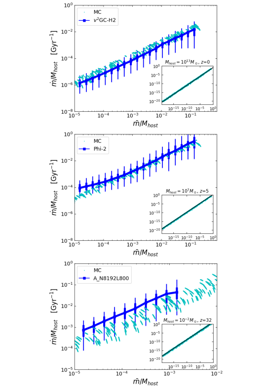
Figure 1: Mass-loss rate of subhalos as a function of orbit-averaged subhalo mass $\overline{m}$ in units of the host mass $M_{\rm host}$ for $M_{\mathrm{host}}=10^{13}M_{\odot}$ and $z=0$ (${\it top}$), $M_{\mathrm{host}}=10^{7}M_{\odot}$ and $z=5$ (${\it middle}$), and $M_{\mathrm{host}}=10^{-2}M_{\odot}$ and $z=32$ (${\it bottom}$). Cyan points show the Monte Carlo simulation results. Blue squares with error bars show the results obtained by $N$-body simulations. Thick error bars correspond to the 50% of the simulated halos around the median, while thin ones to the 90%. We also show the results of the Monte Carlo simulations of wider mass range in inserted panels, which also include the fitting results with Eq. (1), as overwritten solid lines on the Monte Carlo points.

In Figure. 1, we show results of our Monte Carlo simulations. We find that for a large dynamic range of subhalo mass $m$ (over 19 orders of magnitude as shown in the insets) down to very small masses such as $10^{-6}M_{\odot}$, a single power-law function [Eq. (1)] gives a very good fit, which confirms the physical origin of this relation, not just being a simple phenomenological fit.

We compare the results of the Monte Carlo calculations to those of the $N$-body simulations as described in Sec. III.2, which is also shown in Figure. 1 for $\overline{m}/M_{\rm host}\gtrsim 10^{-5}$ ($\overline{m}$ is the orbit-averaged mass of the subhalos), resolved in the $N$-body simulations. At relatively small redshifts for both $M_{\rm host}=10^{13}M_{\odot}$ and $10^{7}M_{\odot}$, we find very good agreement between the two prescriptions. We also check the applicability of the analytical approach by comparing the results with those of $N$-body simulations of small-mass hosts at higher redshift, $z=32$, for which $\eta$ distribution at $z=7$ of Reference. Wetzel:2010kz was adopted. Even at the very high redshift and for very small host mass of $M_{\rm host}=10^{-2}M_{\odot}$, we still find reasonable agreement within differences of factor of a few in $\dot{m}$ between results obtained by the Monte Carlo approaches and the N-body simulations. Although we cannot test the validity of our Monte Carlo approach for $\overline{m}/M_{\rm host}\ll 10^{-5}$ in comparison with the $N$-body simulations, these agreements that have been seen in Figure. 1 from very small to large hosts as well as from very high to low redshifts give us confidence that our analytical prescription captures physics of tidal stripping, and hence can be applied even to the cases with an extremely small mass ratio $\overline{m}/M_{\rm host}$.

From each calculation of $(M_{\mathrm{host}},z)$, we fitted the values of $A$ and $\zeta$ in Eq. (1). We then derived the dependence of $A$ and $\zeta$ on the host mass $M_{\mathrm{host}}$ and $z$ as:

$$\log A = \left[-0.0003\log\left(\frac{M_{\mathrm{host}}}{M_{\odot}}\right)+0.02\right]z$$ (23)

$${}+0.011\log\left(\frac{M_{\mathrm{host}}}{M_{\odot}}\right)-0.354,$$

$$\zeta = \left[0.00012\log\left(\frac{M_{\mathrm{host}}}{M_{\odot}}\right)-0.0033\right]z$$ (24)

$${}-0.0011\log\left(\frac{M_{\mathrm{host}}}{M_{\odot}}\right)+0.026.$$

We obtain the relations, Eqs.(23) and (24), from results of the Monte Carlo simulations that covers the host mass from $M_{\mathrm{host}}=10^{-6}M_{\odot}$ to $10^{16}M_{\odot}$ and the redshift from $z=0$ to $7$.

IV Results

By combining the tidal mass-loss rate (Sec. III) with the analytical prescription for computing density profiles after tidal stripping as well as the subhalo accretion onto evolving hosts (Sec. II), we are able to calculate quantities of interest related to the subhalos. They are the subhalo mass function and the annihilation boost factor, discussed below in Secs. IV.1 and IV.2, respectively.

We first fix the reshift of interest $z_{0}$ and the host mass at that redshift, $M_{0}$. For each set of ($M_{0}$, $z_{0}$), we uniformly sample $m_{\rm acc}$ in logarithmic space between $10^{-6}M_{\odot}$ and $0.1M_{0}$, and $z_{\rm acc}$ between $z_{0}+0.1$ and $10$. Each combination is characterized by a subscript $i$, ($\ln m_{{\rm acc},i}$, $z_{{\rm acc},i}$). Its weight $w_{i}$ is chosen to be proportional to the subhalo accretion rate from the extended Press-Schechter formalism (Appendix C):

$$w_{i}\propto\left(\frac{d^{2}N_{\rm sh}}{d\ln m_{\rm acc}dz_{\rm acc}}\right)_{i}.$$ (25)

This weight is normalized such that

$$\sum_{i}w_{i}=N_{\rm sh,total},$$ (26)

where $N_{\rm sh,total}$ represents the total number of subhalos ever accreted on the given host by the time $z=z_{0}$. It is obtained by numerically integrating $d^{2}N_{\rm sh}/(d\ln m_{\rm acc}dz_{\rm acc})$ [Eq. (52)] over $\ln m_{\rm acc}$ and $z_{\rm acc}$. This way, we essentially approximate the integral of the distribution of $\ln m_{\rm acc}$ and $z_{\rm acc}$ as

$$\int d\ln m_{\rm acc}\int dz_{\rm acc}\frac{d^{2}N_{\rm sh}}{d\ln m_{\rm acc}dz_{\rm acc}}~{}\to~{}\sum_{i}w_{i}.$$ (27)

IV.1 Mass function of subhalos

As discussed in Sec. III.1, the subhalo mass at $z_{0}$ after tidal stripping, $m_{0,i}$, is calculated by integrating Eq. (1) over cosmic time from that corresponding to $z=z_{{\rm acc},i}$ to $z=z_{0}$. The parameters $A$ and $\zeta$ are taken from Eqs. (23) and (24), respectively. For each $i$, we obtain the subhalo concentrations at accretion following the log-normal distribution $P(c_{\rm vir,acc}|m_{{\rm acc},i},z_{{\rm acc},i})$ as discussed in Sec. II and calculate the scale radius $r_{s,i}$ and characteristic density $\rho_{s,i}$ at redshift $z_{\mathrm{acc},i}$, as functions of $c_{\rm vir,acc}$. Those quantities after tidal stripping is then obtained from those before the stripping combined with the stripped mass $m_{0,i}$, as in Sec. II. If the truncation radius, $r_{t,i}$, is found smaller than $0.77r_{s,i}$ at $z=z_{0}$ after the tidal stripping, we exclude the subhalo from calculation of the mass function as it is regarded as completely disrupted.

The subhalo mass function is then constructed as the distribution of $m_{0,i}$ properly weighted by $w_{i}$ with the condition of tidal disruption as follows:

$$\frac{dN_{\rm sh}}{dm} = \sum_{i}w_{i}\delta(m-m_{0,i})$$

$${}\times\int dc_{\rm vir,acc}P(c_{\rm vir,acc}|m_{{\rm acc},i},z_{{\rm acc},i})$$

$${}\times\Theta[r_{t,i}(z_{0}|c_{\rm vir,acc})-0.77r_{s,i}(z_{0}|c_{\rm vir,acc})],$$

where $\delta(x)$ and $\Theta(x)$ are the Dirac delta function and Heaviside step function, respectively.

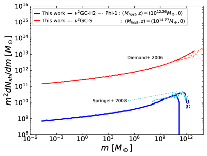
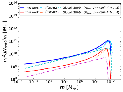
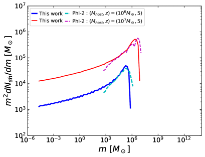
Figure 2: Mass function of subhalos and comparison with the results of numerical simulations. Top: Comparison at $z=0$. Thick (blue) lines correspond to the case of $M_{\mathrm{host}}=1.8\times 10^{12}M_{\odot}$ while thin (red) lines to $5.9\times 10^{14}M_{\odot}$. Solid lines show the mass function obtained in our analytical modelings and dashed lines show those obtained by the N-body simulations in Table 1. Fitting fnctions in Reference. Springel:2008cc for $M_{\mathrm{host}}=1.8\times 10^{12}M_{\odot}$ and in Reference. Diemand:2006ey for $5.9\times 10^{14}M_{\odot}$ are also shown for comparison. Middle: Cases of $M_{\mathrm{host}}=2.3\times 10^{12}M_{\odot}$ at $z=2$ (solid, blue) and $M_{\mathrm{host}}=4.7\times 10^{11}M_{\odot}$ at $z=4$ (thin, red) in comparison again with the simulations in Table 1 and Reference. Giocoli:2009ie . Bottom: Comparison at $z=5$ for the cases of $M_{\mathrm{host}}=10^{6}M_{\odot}$ (solid, blue lines) and $10^{7}M_{\odot}$ (thin, red lines) with the Phi-2 simulations. Note that some of the lines corresponding to our $N$-body simulations extends toward large masses, because halos of various masses around a given geometric mean have been stacked in order to derive the mass functions.

The subhalo mass function has been studied most commonly through $N$-body simulations in the literature. We show $m^{2}dN_{\rm sh}/dm$ obtained by the numerical simulations and by our analytical model [Eq. (LABEL:eq:SHMF)] in Figure. 2. In the top panel of Figure. 2, we compare the subahalo mass function for host masses $M_{\mathrm{host}}=1.8\times 10^{12}M_{\odot}$ and $5.9\times 10^{14}M_{\odot}$ at $z=0$ with the fitting functions to the results of References. Springel:2008cc and Diemand:2006ey , respectively. In both cases, the simulations and analytical models show reasonable agreement, while our model predicts fewer subhalos. We also show the results of $\nu^{2}$GC-S, $\nu^{2}$GC-H2, and Phi-1 simulations, all of which show better agreement with our analytical results. In the middle panel of Figure. 2, we compare the mass function at $z=2$ and $z=4$ with results of Reference. Giocoli:2009ie as well as $\nu^{2}$GC-H2, for the host that has the mass of $M_{\mathrm{host}}=10^{13}M_{\odot}$ at $z=0$. This again shows very good agreement between the two approaches, where the subhalos are resolved in the numerical simulations. Our model can also be applied to cases of even smaller hosts. In the bottom panel of Figure. 2, we compare the subhalo mass function for $M_{\mathrm{host}}=10^{6}M_{\odot}$ and $10^{7}M_{\odot}$ at $z=5$ with the results of the Phi-2 simulations. Down to the resolution limit of the simulations that are around 500–$1000M_{\odot}$, both the calculations agree well. Hence, the subhalo mass functions from our analytical model is well calibrated to the results of the numerical simulations at high masses, and since it is physically motivated, the behavior at low-mass end down to very small masses can also be regarded as reliable.

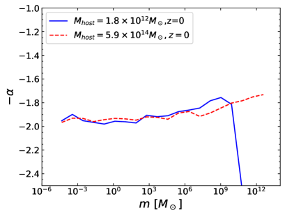
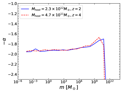
Figure 3: The slope of the subhalo mass function $-\alpha=d\ln(dN_{\rm sh}/dm)/d\ln m$ as a function of $m$. The slope was averaged over mass bins of width $\Delta\log m=1$.

In Figure. 3, we show the slope of the subhalo mass function

$$-\alpha=\frac{d\ln(dN_{\rm sh}/dm)}{d\ln m},$$ (29)

(i.e., $dN_{\rm sh}/dm\propto m^{-\alpha}$) for the same models as in Figure. 2. We find that the slope lies in a range between $-2$ and $-1.8$ for a large range of $m$ except for lower and higher edges where the mass function features cutoffs. This is consistent with one of the findings from the numerical simulations, again confirming validity of our analytical model.

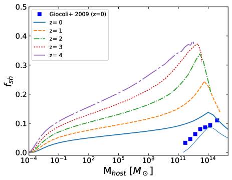
Figure 4: Mass fraction of the host halo in the form of subhalos, $f_{\rm sh}$ as a function of $M_{\rm host}$, for $z=0$, 1, 2, 3, and 4. Blue squares represent the subhalo mass fractions in Reference. Giocoli:2009ie , which are derived using subhalos with masses between $1.73\times 10^{10}h^{-1}M_{\odot}$ and $0.1M_{\mathrm{host}}$. Solid thin line shows the corresponding subhalo mass fraction in our calculation.

Figure 4 shows the mass fraction of the host mass that is contained in the form of the subhalos:

$$f_{\rm sh}=\frac{1}{M_{\rm host}}\int_{10^{-6}M_{\odot}}^{0.1M_{\rm host}}dm\ m\frac{dN_{\rm sh}}{dm}.$$ (30)

At $z=0$, this fraction is smaller than $\sim$10% level up to cluster-size halos. We also find that $f_{\rm sh}$ is larger for higher redshifts, as the effect of tidal mass loss is suppressed compared with the case of $z=0$. In Figure. 4, we also show the results of $N$-body simulations by Reference. Giocoli:2009ie for the subhalo mass fraction between $1.73\times 10^{10}h^{-1}M_{\odot}$ and $0.1M_{\mathrm{host}}$, which is in good agreement with our analytical result for the same quantity.

IV.2 Subhalo boost

IV.2.1 Case of smooth subhalos

The gamma-ray luminosity from dark matter annihilation in the smooth NFW component of the host halo with mass $M$ and redshift $z$ is obtained as

$$L_{\rm host}(M)\propto\int dc_{\rm vir}P(c_{\rm vir}|M,z)\rho_{s}^{2}r_{s}^{3}\left[1-\frac{1}{(1+c_{\rm vir})^{3}}\right],$$ (31)

where $P(c_{\rm vir}|M,z)$ is again the log-normal distribution of the host’s concentration parameter given $M$ and $z$, and the scale radius $r_{s}$ and the characteristic density $\rho_{s}$ are both dependent on $c_{\rm vir}$ as well as on $M$ and $z$. The constant of proportionality of this relation includes particle physics parameters such as the mass and annihilation cross section of dark matter particles, but since here we are interested in the ratio of the luminosities between the subhalos and the host, their dependence cancels out.

Subhalo boost factor quantifies the contribution of all the subhalos to the total annihilation yields compared with the contribution from the host. It is defined as

$$B_{\rm sh}(M)=\frac{L_{\rm sh}^{\rm total}(M)}{L_{\rm host}(M)},$$ (32)

such that the total luminosity from the halo is given as $L_{\rm total}=(1+B_{\rm sh})L_{\rm host}$. The luminosity from a single subhalo $i$ characterized with its accretion mass $m_{{\rm acc},i}$ and redshift $z_{{\rm acc},i}$, as well as its virial concentration $c_{\rm vir,acc}$ is

$$L_{{\rm sh},i}\propto\rho_{s,i}^{2}r_{s,i}^{3}\left[1-\frac{1}{(1+r_{t,i}/r_{s,i})^{3}}\right],$$ (33)

where $r_{s,i}$, $r_{t,i}$, and $\rho_{s,i}$ are the scale radius, truncation radius, and characteristic density of the subhalo $i$ after it experienced the tidal mass loss, and hence they are functions of $m_{{\rm acc},i}$, $z_{{\rm acc},i}$, and $c_{\rm vir,acc}$ as well as the mass of the host $M$ and redshift $z$ (Sec. II). The total subhalo luminosity $L_{\rm sh}^{\rm total}(M)$ is then obtained as the sum of $L_{{\rm sh},i}$ with weight $w_{i}$ and averaged over $c_{\rm vir,acc}$ with its distribution:

$$L_{\rm sh}^{\rm total}(M) = \sum_{i}w_{i}\int dc_{\rm vir,acc}P(c_{\rm vir,acc}|m_{{\rm acc},i},z_{{\rm acc},i})$$

$${}\times L_{{\rm sh},i}(z|c_{\rm vir,acc})$$

$${}\times\Theta[r_{t,i}(z|c_{\rm vir,acc})-0.77r_{s,i}(z|c_{\rm vir,acc})].$$

IV.2.2 Presence of sub-subhalos

The discussions above, especially Eq. (33), are based on the assumption that the density profile of subhalos is given by smooth NFW function. Subhalos, however, contain their own subhalos: i.e., sub-subhalos, which again contain sub-sub-subhalos, and so on. This is because the subhalos, before accreting onto their host, were formed by mergers and accretion of even smaller halos. In the following, we refer to them as subⁿ-subhalos; the discussion above correspond to the case of $n=0$, where subhalos do not include sub-subhalos.

We include the effect of subⁿ-subhalos iteratively. In the case of $n\geq 1$, when a subhalo $i$ accretes at $z_{{\rm acc},i}$ with a mass $m_{{\rm acc},i}$, we give it a sub-subhalo boost $B_{\rm sh}^{(n-1)}(m_{{\rm acc},i},z_{{\rm acc},i})$ obtained from the previous iteration; for $n=1$, it is Eq. (32) evaluated at $m_{{\rm acc},i}$ and $z_{{\rm acc},i}$. After the subhalo exprience the mass loss, its sub-subhalos as well as smooth component are stripped away up to the tidal radius $r_{t,i}$. Since the sub-subhalo distribution (that the gamma-ray brightness profile from the sub-subhalos follows) is flatter than the brightness profile of the subhalo’s smooth component that is proportional to the NFW profile squared, the sub-subhalo boost decreases. In order to quantify this effect, we assume that the sub-subhalos are distributed as $n_{\rm ssh}(r)\propto(r^{2}+r_{s}^{2})^{-3/2}$ (see, e.g., Reference. Ando:2013ff and references therein), and further assuming that $r_{s}$ and $\rho_{s}$ hardly change after mass loss, the total sub-subhalo luminosity enclosed within $r$ is

$$L_{{\rm ssh},i}(<r)\propto\ln\left[\sqrt{1+\left(\frac{r}{r_{s,i}}\right)^{2}}+\frac{r}{r_{s,i}}\right]-\frac{r}{\sqrt{r^{2}+r_{s,i}^{2}}}.$$ (35)

On the other hand, the enclosed luminosity from the smooth NFW component is

$$L_{{\rm sh},i}(<r)\propto 1-\left(1+\frac{r}{r_{s,i}}\right)^{-3}.$$ (36)

The sub-subhalo boost for the subhalo $i$ at redshift $z$ after $n$-th iteration is therefore estimated as

$$B_{{\rm ssh},i}^{(n)}(z) = B_{\rm sh}^{(n-1)}(m_{{\rm acc},i},z_{{\rm acc},i})$$ (37)

$${}\times\frac{L_{{\rm ssh},i}(<r_{t,i})/L_{{\rm ssh},i}(<r_{{\rm vir},i})}{L_{{\rm sh},i}(<r_{t,i})/L_{{\rm sh},i}(<r_{{\rm vir},i})},$$

where $r_{{\rm vir},i}$ is the virial radius of the subhalo $i$ at accretion.

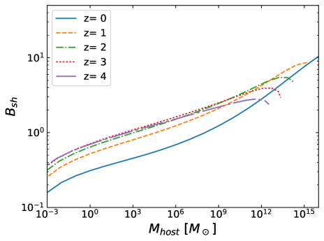
Figure 5: Boost factor $B_{\rm sh}=L_{\rm sh}^{\rm total}/L_{\rm host}$ as a function of the host mass $M_{\mathrm{host}}$ (defined as $M_{200}$) between $10^{-3}M_{\odot}$ and $10^{16}M_{\odot}$ at observation redshifts $z=0$, 1, 2, 3, and 4. The calculations include up to sub³-subhalos.

We finally obtain the subhalo boost factor after $n$-th interation (that takes up to sub^n-1-subhalos into account), $B_{\rm sh}^{(n)}(M,z)$, by combining Eqs. (31)–(LABEL:eq:Lsh_total), but also by multiplying $L_{{\rm sh},i}$ in Eq. (33) with $1+B_{{\rm ssh},i}^{(n)}(z_{0})$ [Eq. (37)]. In this calculation, we consider the subhalos accreted after $z=10$, which assures that we can follow the mass-loss of the subhalos contributing to the boost factor at $z<5$. Figure. 5 shows the boost factor $B_{\rm sh}$ as a function of host mass $M_{\rm host}$ (defined as $M_{200}$) for several redshifts, after fourth iteration that takes up to sub³-subhalos into account. For $z=0$, the subhalo boost increases gradually with the mass of the hosts, and reaches to about a factor of ten for cluster-size halos. The boost for high redshifts is still significant, being on the order of one, for wide range of host masses.

Figure 6: Subhalo boost factor at $z=0$ including subⁿ-subhalos; i.e., $n$-th sub-substructure.

In Figure. 6, we investigate the effect of higher-order substructure: subⁿ-subhalos. Including no sub-substructure ($n=0$) would underestimate the boost by about a factor of a few for massive host halos such as galaxies and clusters. We find that the boost saturates after the third iteration, after which further enhancement is of several percent level.

V Discussion

V.1 Comparison with earlier work

The current work updated an analytical model of Reference. Bartels:2015uba , by (i) implementing the scatter distribution in the concentration-mass relation for both the host and subhalos, (ii) calibrating the subhalo mass-loss rate down to extremely small mass ratio $m/M$ using the Monte Carlo simulations of the tidal stripping, (iii) extending the calculations of the boost factor as well as the subhalo mass function beyond $z=0$, and (iv) including sub-subhalos and beyond. They are all essential ingredients to improve the accuracy of the subhalo modeling, and hence the current work is regarded as direct update of Reference. Bartels:2015uba . As the quantitative outcome, we find that the subhalo boost without contribution from sub-subhalos ($n=0$) is consistent with the result of Reference. Bartels:2015uba . Our result including up to sub³-subhalos further enhances the boost by a factor of 2–3 for large halos, and extends the calculation down to $10^{-4}M_{\odot}$.

The effect of tidal stripping on the annihilation boost has also been studied in References. Zavala:2015ura ; Moline:2016pbm by using different approaches, but they both have reached a similar conclusion to that of Reference. Bartels:2015uba . In particular, Reference. Moline:2016pbm relied directly on $N$-body simulations to claim that subhalos are more concentrated than field halos of the equal mass, and hence, the annihilation boost is larger than previous estimates by, e.g., Reference. Sanchez-Conde:2013yxa . One of the great advantages of directly using the results from $N$-body simulations is its accuracy when the discussion concerns the resolved regime. However, each simulation is computationally demanding, and thus, it is not easy to generalize the discussion to wider ranges of host masses and redshifts. In fact, in order to compute the subhalo boost factor as a function of the host mass, Reference. Moline:2016pbm had to combine the subhalo concentration-mass relation with the subhalo mass function, for the latter of which a few phonomenological fitting functions calibrated with other simulations were adopted. Hence, the boost factor as its outcome shows a very large range of uncertainties depending on what model of the mass function one adopts. In our analytical approach, on the other hand, we are able to perform physics-based computations of the subhalo boost factor and mass function in a self-consistent manner, for very wide ranges of masses and redshifts.

References Kamionkowski:2008vw ; Kamionkowski:2010mi developed an analytical model assuming self-similarity of the substructures, computed the probability distribution function of the dark matter density that has a power-law tail, and calibrated it with numerical simulations of the Galactic halo. The annihilation boost factor within the volume of the virial radius of $\sim$200 kpc was found to be $\sim$10, which is slightly larger than our result. This, however, agrees with our result based on a different model of the concentration-mass relation (see Sec. V.3).

Reference Stref:2016uzb modeled dark matter subhalos in a Milky-Way-like halo at $z=0$ by including the effect of the disk shocking as well as the tidal stripping. Our result of the annihilation boost factor is consistent with that of Reference. Stref:2016uzb after integrating over the entire volume of the halo and assuming the subhalo mass function of $\propto m^{-1.9}$. Our discussion in Sec. III can be expanded to accommodate the spatial distribution of subhalos, but doing so and comparing the result with that of Reference. Stref:2016uzb would include proper modeling of the baryonic component, which is beyond the scope of the present work.

V.2 A case without tidal disruption

Reference vandenBosch:2017ynq recently pointed out that the tidal disruption for the subhalos with $r_{t}<0.77r_{s}$ might be a numerical artifact, and many more subhalos even with much smaller truncation radius $r_{t}$ could survive against the tidal disruption. In this paper, we do not argue for or against the claim of Reference. vandenBosch:2017ynq , but simply study the implication of the claim as an optimistic example. To this end, we repeated the boost calculations without implementing the constraint $r_{t}>0.77r_{s}$; i.e., all the subhalos survive no matter how much mass they lose due to the tidal stripping. We find that the obtained boost factor hardly changes at any redshift.

V.3 Dependence on the concentration-mass relation

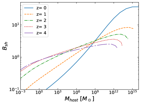
Figure 7: The same as Figure. 5, but for the concentration-mass relation in Reference. Okoli:2015dta .

In our calculations of the boost factor, we adopted the mass-concentration relation in Reference. Correa:2015dva as the canonical model. Their derivation is based on the analysis with $N$-body simulations. Reference Okoli:2015dta proposed a different concentration-mass relation based on analytical considerations, which expect higher concentration especially around $z=0$. In order to compare the dependence of the boost factor on the different concentration-mass relations, we also calculated the boost factor adopting the relation in Reference. Okoli:2015dta . In Figure. 7, we show that the boost factor enhances by more than a fector of a few if we adopt the concentration-mass relation of Reference. Okoli:2015dta instead of that of Reference. Correa:2015dva . Obtained boost factor directly reflects the difference of the concentrations at around $z=0$. We do not discuss the feasibility of these concentrations since that is beyond the scope of this paper. Our results show that deeper understanding of the concentration-mass relation is necessary to obtain the boost factor corresponding to the actual situations.

In Reference. Gosenca:2017ybi , there are some discussions about the mass-concentration relation and the primordial curvature perturbations in the early Universe. If primordial power spectrum has a feature that gives rise to ultra-compact minihaloes, it may boost dark matter annihilation even more significantly by changing density profiles and concentration-mass relation. Although evaluating the subhalo boost for these specific models is beyond the scope of our work, we note that such a significant boost predicted by References. Gosenca:2017ybi ; Delos:2017thv may already be constrained very strongly using the existing gamma-ray data.

V.4 Contriubtion to the isotropic gamma-ray background

One of the advantages of our analytical model of the subhalo boost is capability of calculating the isotropic gamma-ray background (IGRB) from dark matter annihilation, since we can compute boost factors for various host masses and the wide range of redshifts, self-consistently. The intensity of IGRB was most recently measured with Fermi-LAT Ackermann:2014usa , which was then used to constrain dark matter annihilation cross section (e.g., Ackermann:2015tah ).

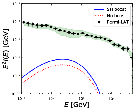
Figure 8: Contriubtion to the IGRB intensity measured by Fermi-LAT from dark matter annihilation for $\langle\sigma v\rangle=2.2\times 10^{-26}$ cm³ s^-1, $m_{\chi}=100$ GeV, and $b\bar{b}$ final state. The solid (dotted) curve shows the case of the subhalo boost (no boost).

We followed the “halo model” approach of Reference. Ando:2013ff to compute the IGRB contribution from dark matter annihilation, but by applying the results of the annihialtion boost factor from our analytical model (Figure. 5) as well as by including scatter of the concentration-mass relation. Figure 8 shows the IGRB intensity from dark matter annihilation in the case of the canonical annihilation cross section for thermal freezeout scenario, $\langle\sigma v\rangle\simeq 2\times 10^{-26}$ cm³ s^-1 Steigman:2012nb , dark matter mass of $m_{\chi}=100$ GeV, and $b\bar{b}$ final state of the annihilation ($\chi\chi\to b\bar{b}$). Our boost model enhances the IGRB intensity by a factor of a few compared with the case of no subhalo boost. Note that contribution from the Galactic subhalos (e.g., Ando:2009fp ) is not included, and hence our estimate is conservative.

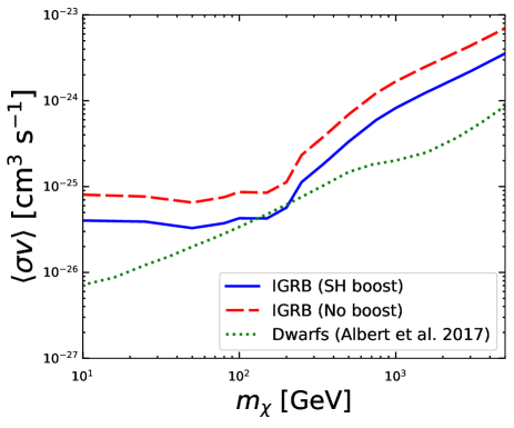
Figure 9: Upper limits on dark matter annihilation cross section at 95% confidence level as a function of dark matter mass for $b\bar{b}$ final state. Solid and dashed curves are for the canonical boost model and without subhalo boost, respectively. For comparison, the result of the latest joint-likelihood analysis of 41 dwarfs Fermi-LAT:2016uux are shown as a dotted curve.

We then performed a simple analysis of the Fermi-LAT IGRB data Ackermann:2015tah . We included two components: (1) dark matter annihilation of a given mass $m_{\chi}$ and assuming a $b\bar{b}$ final states, and (2) an “astrophysical” power-law component with a cutoff, for which we adopt the best-fit spectral shape, $I_{\rm astro}(E)\propto E^{-2.32}\exp(-E/279~{}{\rm GeV})$ Ackermann:2015tah . By adopting normalizations of these components as two free parameters for the fit, we performed a $\chi^{2}$ analysis in order to obtain the upper limits on $\langle\sigma v\rangle$. For the IGRB data, we adopt those for a foreground model “A” in Reference. Ackermann:2015tah , but treat statistical and systematic uncertainties as independent errors. Figure 9 shows the upper limits on $\langle\sigma v\rangle$ at 95% confidence level ($\Delta\chi^{2}=2.71$) using our canonical boost model as well as the case of no boost. Our updated boost model improves the limits by a factor of a few nearly indepently of dark matter mass (see also, e.g., References. Cholis:2013lwa ; DiMauro:2015tfa for earlier results). This enhancement is calculated consistently as our formalism automatically computes all the subhalo properties at once including mass function and the boost factor. We also compare our limits with the latest results of the joint likelihood analysis of 41 dwarf spheroidal galaxies Fermi-LAT:2016uux , which set the benchmark as the most robust constraints on dark matter annihilation.

Although some improvements of the limit obtained from the observations of dwarf spheroidal galaxies also can be expected, we conservatively neglect this contribution according to the discussion in Reference. Bartels:2015uba . We find that the IGRB limits with our boost model are competitive to the dwarf bounds for dark matter massese at $\sim$200 GeV. Note that more accurate limits should include uncertainties coming from modeling of the astrophysical contributions. Further consideration is needed in order to obtain correct values, which is slated for future works. (See also Reference. Hutten:2017cyu for a detailed discussion on various sources of uncertainties.)

The small-scale angular power spectrum of the IGRB has also been measured with Fermi-LAT Fornasa:2016ohl , which provides yet another avenue to constrain dark matter annihilation Ando:2005xg ; Ando:2013ff as well as high-energy astrophysical sources Ando:2006cr ; Ando:2017alx . It is also pointed out that taking cross correlations with local gravitational tracers such as galaxy catalogs is a promising way along the same line Ando:2013xwa ; Ando:2014aoa ; Fornengo:2013rga . Since these anisotropy constraints are more sensitive to the dark matter distribution at smaller redshifts and in larger hosts, the effect of the subhalo boost is expected to be even more important than for the IGRB intensity. A dedicated investigation is beyond the scope of this work and hence reserved as subject in a future paper. We also note that our updated boost model will impact the result of stacking analysis of nearby galaxy groups Lisanti:2017qlb , which relied on the boost model of Reference. Bartels:2015uba .

VI Conclustions

We can access the substructure of dark matter halos which is beyond the resolutions of the numerical simulations by taking analytical approach on the modeling of the tidal mass loss of the subhalos. We analytically modeled the mass loss of subhalos under the gravitational potential of their hosts, following the evolution of both the host and subhalos in a self-consistent way. In order to take distributions of the concentrations of the hosts, orbits and concentrations of subhalos into account, we conducted Monte Carlo simulations. We find that the mass loss of the subhalos are well described with Eq.  (1) down to the scale of $m/M_{\mathrm{host}}\sim{\cal O}(10^{-19})$, and well agree with results of $N$-body simulations.

Combining the derived relation about the subhalo mass loss with analytical models for mass and redshift distributions of accreting subhalos, we calculated the subhalo mass functions and the boost factor for dark matter annihilation. We showed that mass functions of subhalos derived in our analytical modeling are consistent with those obtained in $N$-body simulations down to their resolution limits. From our model of the subhalo boost of dark matter annihilation, we expect enhancement in the gamma-ray signals by up to a factor of $\sim$10 because of the remaining substructures in larger halos, predicting promising opportunities for detecting particle dark matter in future gamma-ray observations. Including substructures in the subhalos will give important contribution to the annihiation boost up to a factor of a few.

The results of our calculations are consistent with both earlier analytical and numerical approaches, but are applicable to much wider (and arbitrary) range of host masses and redshifts, and hence can be used to predict gamma-ray flux from dark matter annihilation in various halos at any redshifts. As an example, we computed the contribution to the isotropic gamma-ray background from our boost model. We find that the presence of subhalos (and their substructures) enhace the gamma-ray intensity by a factor of a few, and hence the limits on the annihilation cross section improves by the same factor, excluding region of $\langle\sigma v\rangle\gtrsim 4\times 10^{-26}$ cm³ s^-1 for dark matter masses smaller than $\sim$200 GeV.

Appendix A Mass evolution of host halos

In order to calculate the evolution of subhalos, we first specify how the hosts that are not in a even larger halo evolve. Reference. Correa:2014xma derive the relations about the mass accretion history of the halos $M(z|M_{0},z=0)$, i.e., the mass of the halo at redshift $z$, whose mass is $M_{0}$ at $z=0$:

$$M(z|M_{0},z=0)=M_{0}(1+z)^{\alpha}\exp(\beta z),$$ (38)

with

$$\beta = -g(M_{0}),$$ (39)

$$\alpha = \left[\frac{1.686\sqrt{2/\pi}}{D^{2}(z=0)}\left.\frac{dD}{dz}\right|_{z=0}+1\right]g(M_{0}),$$ (40)

$$g(M_{0}) = \left[S(M_{0}/q)-S(M_{0})\right]^{-1/2},$$ (41)

$$q = 4.137\tilde{z}_{f}^{-0.9476},$$ (42)

$$\tilde{z}_{f} = -0.0064(\log M_{0})^{2}+0.0237(\log M_{0})$$ (43)

$$+1.8837,$$

where $D(z)$ and $S(M)\equiv\sigma^{2}(M)$ are the growth function and the variance of the matter distribution at mass scale $M$ and $z=0$, respectively. We adopt fitting functions of both $D(z)$ and $\sigma(M)$ from Reference. Ludlow:2016ifl . Eq. (38) is generalized to determine the mass of halos $M(z|M(z_{i}),z_{i})$ at redshift $z$, whose mass was $M(z_{i})$ at redshift $z_{i}$ Correa:2015dva :

$$M(z|M(z_{i}),z_{i})=M(z_{i})(1+z-z_{i})^{\alpha}\exp(\beta(z-z_{i})),$$ (44)

with replacing $M_{0}$ with $M(z_{i})$ in Eqs. (39),(40) and (41). These relations enable us to follow back the evolutions of the hosts starting from any redshift adopting the generalized equations.

Appendix B Concentration-mass relation of the field halos

We here summarize the concentration-mass relation $c_{200}(M_{200})$ for the field halos based on Reference. Correa:2015dva , which is adopted throughout this paper. We take the fitted values corresponding to the Planck cosomlogy.

For $z\leq 4$

$$\log c_{200}=\alpha+\beta\log\left(\frac{M_{200}}{M_{\odot}}\right)\left[1+\gamma\log^{2}\left(\frac{M_{200}}{M_{\odot}}\right)\right],$$ (45)

where

$$\alpha = 1.7543-0.2766(1+z)+0.02039(1+z)^{2},$$ (46)

$$\beta = 0.2753+0.00351(1+z)-0.3038(1+z)^{0.0269},$$

$$\gamma = -0.01537+0.02102(1+z)^{-0.1475},$$ (48)

and for $z>4$,

$$\log c_{200}=\alpha+\beta\log\left(\frac{M_{200}}{M_{\odot}}\right),$$ (49)

where

$$\alpha = 1.3081-0.1078(1+z)+0.00398(1+z)^{2},$$ (50)

$$\beta = 0.0223-0.0944(1+z)^{-0.3907}.$$ (51)

Appendix C Subhalo accretion rate

With the understanding of the growth history of certain hosts, we know the distributions of the mass and redshift of the accreting subhalos on that host. Reference. Yang:2011rf studied the mass accretion history, and obtained the distribution $d^{2}N_{\rm sh}/(d\ln m_{\mathrm{acc}}dz_{\mathrm{acc}})$: the number of subhalos accreted onto the host per unit logarithmic mass range around $\ln m_{\rm acc}$ and per unit redshift range around accretion redshift $z_{\rm acc}$:

$$\frac{d^{2}N_{sh}}{d\ln m_{\mathrm{acc}}dz_{\mathrm{acc}}}={\cal F}(s_{\mathrm{acc}},\delta_{\mathrm{acc}}|S_{0},\delta_{0};\overline{M}_{\mathrm{acc}})\frac{ds_{\mathrm{acc}}}{dm_{\mathrm{acc}}}\frac{d\overline{M}_{\mathrm{acc}}}{dz_{\mathrm{acc}}},$$ (52)

where following the convention of Reference. Yang:2011rf , $s_{\mathrm{acc}}$ and $\delta_{\mathrm{acc}}$ are used to parameterize the mass and redshift, respectively, since they are defined as $s_{\mathrm{acc}}\equiv\sigma^{2}(m_{\mathrm{acc}},z=0)$ and $\delta_{\mathrm{acc}}=\delta_{c}(z_{\mathrm{acc}})=1.686/D(z_{\mathrm{acc}})$ Ludlow:2016ifl . Similarly, for the host, we adopt $S_{0}=\sigma^{2}(M_{0},z=0)$ and $\delta_{0}=\delta_{\rm sc}(z_{0})$ to characterize the mass $M_{0}$ and redshift $z_{0}$ as a boundary condition. The mass of the host $M_{\rm acc}$ at the accretion redshift $z_{\rm acc}$ (that eventually evolves to $M_{0}$ at $z_{0}$) follows the probability distribution $P(M_{\rm acc}|S_{0},\delta_{0})$, for which we adopt a log-normal distribution with a logarithmic mean $\overline{M}_{\mathrm{acc}}=M(z_{\mathrm{acc}}|M_{0},z_{0})$ [Eq. 44] and a logarithmic dispersion

$$\sigma_{\log M_{\rm acc}}=0.12-0.15\log\left(\frac{{M}_{\mathrm{acc}}}{M_{0}}\right).$$ (53)

The definition of the function ${\cal F}$ in Eq. (52) is

$${\cal F}(s_{\mathrm{acc}},\delta_{\mathrm{acc}}|S_{0},\delta_{0};\overline{M}_{\mathrm{acc}})$$

$$= \int\Phi(s_{\mathrm{acc}}.\delta_{\mathrm{acc}}|S_{0},\delta_{0};{M}_{\mathrm{acc}})P({M}_{\mathrm{acc}}|S_{0},\delta_{0})d{M}_{\mathrm{acc}},$$

$$\Phi(s_{\mathrm{acc}},\delta_{\mathrm{acc}}|S_{0},\delta_{0};{M}_{\mathrm{acc}})$$

$$= \left[\int^{\infty}_{S(m_{\mathrm{max}})}F(s_{\mathrm{acc}},\delta_{\mathrm{acc}}|S_{0},\delta_{0};{M}_{\mathrm{acc}})ds_{\mathrm{acc}}\right]^{-1}$$

$$\times\begin{cases}F(s_{\mathrm{acc}},\delta_{\mathrm{acc}}|S_{0},\delta_{0};{M}_{\mathrm{acc}}),&(m_{\mathrm{acc}}\leq m_{\mathrm{max}}),\\ 0,&(\mathrm{otherwise}),\end{cases}$$

$$F(s_{\mathrm{acc}},\delta_{\mathrm{acc}}|S_{0},\delta_{0};{M}_{\mathrm{acc}})$$ (56)

$$= \frac{1}{\sqrt{2\pi}}\frac{\delta_{\mathrm{acc}}-\delta_{M}}{(s_{\mathrm{acc}}-S_{M})^{3/2}}\exp\left[-\frac{(\delta_{\mathrm{acc}}-\delta_{M})^{2}}{2(s_{\mathrm{acc}}-S_{M})}\right],$$

where $m_{\mathrm{max}}=\min[{M}_{\mathrm{acc}},M_{0}/2]$ and $M_{\mathrm{max}}=\min[{M}_{\mathrm{acc}}+m_{\mathrm{max}},M_{0}]$ are introduced such that the mass hierarchy of the host mass before and after subhalo accretions is assured, $S_{M}=\sigma_{M}^{2}(M_{\mathrm{max}})$ and $\delta_{M}$ is defined as $\delta_{\rm sc}(z)$ at a redshift at which $M=M_{\rm max}$. The equations above determine the distributions of accreting subhalos $d^{2}N_{\mathrm{sh}}/(d\ln m_{\mathrm{acc}}dz_{\mathrm{acc}})$ for arbitrary hosts.

References

- (1) P. J. E. Peebles, “Large scale background temperature and mass fluctuations due to scale invariant primeval perturbations,” Astrophys. J. 263 (1982) L1–L5.
- (2) Planck Collaboration, P. A. R. Ade et al., “Planck 2015 results. XIII. Cosmological parameters,” Astron. Astrophys. 594 (2016) A13, arXiv:1502.01589 [astro-ph.CO].
- (3) T. S. van Albada, J. N. Bahcall, K. Begeman, and R. Sancisi, “The Distribution of Dark Matter in the Spiral Galaxy NGC-3198,” Astrophys. J. 295 (1985) 305–313.
- (4) P. Salucci and A. Borriello, “The intriguing distribution of dark matter in galaxies,” Lect. Notes Phys. 616 (2003) 66–77, arXiv:astro-ph/0203457 [astro-ph].
- (5) D. Clowe, A. Gonzalez, and M. Markevitch, “Weak lensing mass reconstruction of the interacting cluster 1E0657-558: Direct evidence for the existence of dark matter,” Astrophys. J. 604 (2004) 596–603, arXiv:astro-ph/0312273 [astro-ph].
- (6) G. Jungman, M. Kamionkowski, and K. Griest, “Supersymmetric dark matter,” Phys. Rept. 267 (1996) 195–373, arXiv:hep-ph/9506380 [hep-ph].
- (7) J. M. Gaskins, “A review of indirect searches for particle dark matter,” Contemp. Phys. 57 no. 4, (2016) 496–525, arXiv:1604.00014 [astro-ph.HE].
- (8) S. Hofmann, D. J. Schwarz, and H. Stoecker, “Damping scales of neutralino cold dark matter,” Phys. Rev. D64 (2001) 083507, arXiv:astro-ph/0104173 [astro-ph].
- (9) A. M. Green, S. Hofmann, and D. J. Schwarz, “The power spectrum of SUSY - CDM on sub-galactic scales,” Mon. Not. Roy. Astron. Soc. 353 (2004) L23, arXiv:astro-ph/0309621 [astro-ph].
- (10) S. Profumo, K. Sigurdson, and M. Kamionkowski, “What mass are the smallest protohalos?,” Phys. Rev. Lett. 97 (2006) 031301, arXiv:astro-ph/0603373 [astro-ph].
- (11) R. Diamanti, M. E. C. Catalan, and S. Ando, “Dark matter protohalos in a nine parameter MSSM and implications for direct and indirect detection,” Phys. Rev. D92 no. 6, (2015) 065029, arXiv:1506.01529 [hep-ph].
- (12) F. C. van den Bosch, G. Tormen, and C. Giocoli, “The Mass function and average mass loss rate of dark matter subhaloes,” Mon. Not. Roy. Astron. Soc. 359 (2005) 1029–1040, arXiv:astro-ph/0409201 [astro-ph].
- (13) C. Giocoli, L. Pieri, and G. Tormen, “Analytical Approach to Subhaloes Population in Dark Matter Haloes,” Mon. Not. Roy. Astron. Soc. 387 (2008) 689–697, arXiv:0712.1476 [astro-ph].
- (14) F. Jiang and F. C. van den Bosch, “Statistics of dark matter substructure – I. Model and universal fitting functions,” Mon. Not. Roy. Astron. Soc. 458 no. 3, (2016) 2848–2869, arXiv:1403.6827 [astro-ph.CO].
- (15) J. Penarrubia and A. J. Benson, “Effects of dynamical evolution on the distribution of substructures,” Mon. Not. Roy. Astron. Soc. 364 (2005) 977–989, arXiv:astro-ph/0412370 [astro-ph].
- (16) L. Gao, S. D. M. White, A. Jenkins, F. Stoehr, and V. Springel, “The Subhalo populations of lambda-CDM dark halos,” Mon. Not. Roy. Astron. Soc. 355 (2004) 819, arXiv:astro-ph/0404589 [astro-ph].
- (17) J. Diemand, M. Kuhlen, and P. Madau, “Formation and evolution of galaxy dark matter halos and their substructure,” Astrophys. J. 667 (2007) 859–877, arXiv:astro-ph/0703337 [astro-ph].
- (18) C. Giocoli, G. Tormen, and F. C. v. d. Bosch, “The Population of Dark Matter Subhaloes: Mass Functions and Average Mass Loss Rates,” Mon. Not. Roy. Astron. Soc. 386 (2008) 2135–2144, arXiv:0712.1563 [astro-ph].
- (19) K. Dolag, S. Borgani, G. Murante, and V. Springel, “Substructures in hydrodynamical cluster simulations,” Mon. Not. Roy. Astron. Soc. 399 (2009) 497, arXiv:0808.3401 [astro-ph].
- (20) V. Springel, J. Wang, M. Vogelsberger, A. Ludlow, A. Jenkins, A. Helmi, J. F. Navarro, C. S. Frenk, and S. D. M. White, “The Aquarius Project: the subhalos of galactic halos,” Mon. Not. Roy. Astron. Soc. 391 (2008) 1685–1711, arXiv:0809.0898 [astro-ph].
- (21) F. C. van den Bosch, G. Ogiya, O. Hahn, and A. Burkert, “Disruption of Dark Matter Substructure: Fact or Fiction?,” Mon. Not. Roy. Astron. Soc. 474 no. 3, (2018) 3043–3066, arXiv:1711.05276 [astro-ph.GA].
- (22) J. Diemand, M. Kuhlen, and P. Madau, “Dark matter substructure and gamma-ray annihilation in the Milky Way halo,” Astrophys. J. 657 (2007) 262–270, arXiv:astro-ph/0611370 [astro-ph].
- (23) L. E. Strigari, S. M. Koushiappas, J. S. Bullock, and M. Kaplinghat, “Precise constraints on the dark matter content of Milky Way dwarf galaxies for gamma-ray experiments,” Phys. Rev. D75 (2007) 083526, arXiv:astro-ph/0611925 [astro-ph].
- (24) L. Pieri, G. Bertone, and E. Branchini, “Dark Matter Annihilation in Substructures Revised,” Mon. Not. Roy. Astron. Soc. 384 (2008) 1627, arXiv:0706.2101 [astro-ph].
- (25) T. E. Jeltema and S. Profumo, “Searching for Dark Matter with X-ray Observations of Local Dwarf Galaxies,” Astrophys. J. 686 (2008) 1045, arXiv:0805.1054 [astro-ph].
- (26) T. Ishiyama, “Hierarchical Formation of Dark Matter Halos and the Free Streaming Scale,” Astrophys. J. 788 (2014) 27, arXiv:1404.1650 [astro-ph.CO].
- (27) R. Bartels and S. Ando, “Boosting the annihilation boost: Tidal effects on dark matter subhalos and consistent luminosity modeling,” Phys. Rev. D92 no. 12, (2015) 123508, arXiv:1507.08656 [astro-ph.CO].
- (28) C. A. Correa, J. S. B. Wyithe, J. Schaye, and A. R. Duffy, “The accretion history of dark matter haloes – I. The physical origin of the universal function,” Mon. Not. Roy. Astron. Soc. 450 no. 2, (2015) 1514–1520, arXiv:1409.5228 [astro-ph.GA].
- (29) J. F. Navarro, C. S. Frenk, and S. D. M. White, “A Universal density profile from hierarchical clustering,” Astrophys. J. 490 (1997) 493–508, arXiv:astro-ph/9611107 [astro-ph].
- (30) G. L. Bryan and M. L. Norman, “Statistical properties of x-ray clusters: Analytic and numerical comparisons,” Astrophys. J. 495 (1998) 80, arXiv:astro-ph/9710107 [astro-ph].
- (31) C. A. Correa, J. S. B. Wyithe, J. Schaye, and A. R. Duffy, “The accretion history of dark matter haloes – III. A physical model for the concentration–mass relation,” Mon. Not. Roy. Astron. Soc. 452 no. 2, (2015) 1217–1232, arXiv:1502.00391 [astro-ph.CO].
- (32) W. Hu and A. V. Kravtsov, “Sample variance considerations for cluster surveys,” Astrophys. J. 584 (2003) 702–715, arXiv:astro-ph/0203169 [astro-ph].
- (33) T. Ishiyama, J. Makino, S. Portegies Zwart, D. Groen, K. Nitadori, S. Rieder, C. de Laat, S. McMillan, K. Hiraki, and S. Harfst, “The Cosmogrid Simulation: Statistical Properties of Small Dark Matter Halos,” Astrophys. J. 767 (2013) 146, arXiv:1101.2020 [astro-ph.CO].
- (34) J. Penarrubia, A. J. Benson, M. G. Walker, G. Gilmore, A. McConnachie, and L. Mayer, “The impact of dark matter cusps and cores on the satellite galaxy population around spiral galaxies,” Mon. Not. Roy. Astron. Soc. 406 (2010) 1290, arXiv:1002.3376 [astro-ph.GA].
- (35) E. Hayashi, J. F. Navarro, J. E. Taylor, J. Stadel, and T. R. Quinn, “The Structural evolution of substructure,” Astrophys. J. 584 (2003) 541–558, arXiv:astro-ph/0203004 [astro-ph].
- (36) X. Yang, H. J. Mo, Y. Zhang, and F. C. v. d. Bosch, “An analytical model for the accretion of dark matter subhalos,” Astrophys. J. 741 (2011) 13, arXiv:1104.1757 [astro-ph.CO].
- (37) A. R. Wetzel, “On the Orbits of Infalling Satellite Halos,” Mon. Not. Roy. Astron. Soc. 412 (2011) 49, arXiv:1001.4792 [astro-ph.CO].
- (38) T. Ishiyama, M. Enoki, M. A. R. Kobayashi, R. Makiya, M. Nagashima, and T. Oogi, “The GC simulations: Quantifying the dark side of the universe in the Planck cosmology,” Publ. Astron. Soc. Jap. 67 no. 4, (2015) 61, arXiv:1412.2860 [astro-ph.CO].
- (39) Planck Collaboration, P. A. R. Ade et al., “Planck 2013 results. XVI. Cosmological parameters,” Astron. Astrophys. 571 (2014) A16, arXiv:1303.5076 [astro-ph.CO].
- (40) T. Ishiyama, T. Fukushige, and J. Makino, “GreeM : Massively Parallel TreePM Code for Large Cosmological N-body Simulations,” Publ. Astron. Soc. Jap. 61 (2009) 1319–1330, arXiv:0910.0121 [astro-ph.IM].
- (41) T. Ishiyama, K. Nitadori, and J. Makino, “4.45 Pflops Astrophysical N-Body Simulation on K computer – The Gravitational Trillion-Body Problem,” arXiv:1211.4406 [astro-ph.CO].
- (42) P. S. Behroozi, R. H. Wechsler, and H.-Y. Wu, “The Rockstar Phase-Space Temporal Halo Finder and the Velocity Offsets of Cluster Cores,” Astrophys. J. 762 (2013) 109, arXiv:1110.4372 [astro-ph.CO].
- (43) P. S. Behroozi, R. H. Wechsler, H.-Y. Wu, M. T. Busha, A. A. Klypin, and J. R. Primack, “Gravitationally Consistent Halo Catalogs and Merger Trees for Precision Cosmology,” Astrophys. J. 763 (2013) 18, arXiv:1110.4370 [astro-ph.CO].
- (44) R. Makiya, M. Enoki, T. Ishiyama, M. A. R. Kobayashi, M. Nagashima, T. Okamoto, K. Okoshi, T. Oogi, and H. Shirakata, “The New Numerical Galaxy Catalog (GC): An updated semi-analytic model of galaxy and active galactic nucleus formation with large cosmological N-body simulations,” Publ. Astron. Soc. Jap. 68 no. 2, (2016) 25, arXiv:1508.07215 [astro-ph.GA].
- (45) J. Diemand, M. Kuhlen, and P. Madau, “Early supersymmetric cold dark matter substructure,” Astrophys. J. 649 (2006) 1–13, arXiv:astro-ph/0603250 [astro-ph].
- (46) C. Giocoli, G. Tormen, R. K. Sheth, and F. C. van den Bosch, “The Substructure Hierarchy in Dark Matter Haloes,” Mon. Not. Roy. Astron. Soc. 404 (2010) 502–517, arXiv:0911.0436 [astro-ph.CO].
- (47) S. Ando and E. Komatsu, “Constraints on the annihilation cross section of dark matter particles from anisotropies in the diffuse gamma-ray background measured with Fermi-LAT,” Phys. Rev. D87 no. 12, (2013) 123539, arXiv:1301.5901 [astro-ph.CO].
- (48) J. Zavala and N. Afshordi, “Universal clustering of dark matter in phase space,” Mon. Not. Roy. Astron. Soc. 457 no. 1, (2016) 986–992, arXiv:1508.02713 [astro-ph.CO].
- (49) Á. Moliné, M. A. Sánchez-Conde, S. Palomares-Ruiz, and F. Prada, “Characterization of subhalo structural properties and implications for dark matter annihilation signals,” Mon. Not. Roy. Astron. Soc. 466 no. 4, (2017) 4974–4990, arXiv:1603.04057 [astro-ph.CO].
- (50) M. A. Sánchez-Conde and F. Prada, “The flattening of the concentration–mass relation towards low halo masses and its implications for the annihilation signal boost,” Mon. Not. Roy. Astron. Soc. 442 no. 3, (2014) 2271–2277, arXiv:1312.1729 [astro-ph.CO].
- (51) M. Kamionkowski and S. M. Koushiappas, “Galactic substructure and direct detection of dark matter,” Phys. Rev. D77 (2008) 103509, arXiv:0801.3269 [astro-ph].
- (52) M. Kamionkowski, S. M. Koushiappas, and M. Kuhlen, “Galactic Substructure and Dark Matter Annihilation in the Milky Way Halo,” Phys. Rev. D81 (2010) 043532, arXiv:1001.3144 [astro-ph.GA].
- (53) M. Stref and J. Lavalle, “Modeling dark matter subhalos in a constrained galaxy: Global mass and boosted annihilation profiles,” Phys. Rev. D95 no. 6, (2017) 063003, arXiv:1610.02233 [astro-ph.CO].
- (54) C. Okoli and N. Afshordi, “Concentration, Ellipsoidal Collapse, and the Densest Dark Matter haloes,” Mon. Not. Roy. Astron. Soc. 456 no. 3, (2016) 3068–3078, arXiv:1510.03868 [astro-ph.CO].
- (55) M. Gosenca, J. Adamek, C. T. Byrnes, and S. Hotchkiss, “3D simulations with boosted primordial power spectra and ultracompact minihalos,” Phys. Rev. D96 no. 12, (2017) 123519, arXiv:1710.02055 [astro-ph.CO].
- (56) M. S. Delos, A. L. Erickcek, A. P. Bailey, and M. A. Alvarez, “Are ultracompact minihalos really ultracompact?,” Phys. Rev. D97 no. 4, (2018) 041303, arXiv:1712.05421 [astro-ph.CO].
- (57) Fermi-LAT Collaboration, M. Ackermann et al., “The spectrum of isotropic diffuse gamma-ray emission between 100 MeV and 820 GeV,” Astrophys. J. 799 (2015) 86, arXiv:1410.3696 [astro-ph.HE].
- (58) Fermi-LAT Collaboration, M. Ackermann et al., “Limits on Dark Matter Annihilation Signals from the Fermi LAT 4-year Measurement of the Isotropic Gamma-Ray Background,” JCAP 1509 no. 09, (2015) 008, arXiv:1501.05464 [astro-ph.CO].
- (59) G. Steigman, B. Dasgupta, and J. F. Beacom, “Precise Relic WIMP Abundance and its Impact on Searches for Dark Matter Annihilation,” Phys. Rev. D86 (2012) 023506, arXiv:1204.3622 [hep-ph].
- (60) S. Ando, “Gamma-ray background anisotropy from galactic dark matter substructure,” Phys. Rev. D80 (2009) 023520, arXiv:0903.4685 [astro-ph.CO].
- (61) DES, Fermi-LAT Collaboration, A. Albert et al., “Searching for Dark Matter Annihilation in Recently Discovered Milky Way Satellites with Fermi-LAT,” Astrophys. J. 834 no. 2, (2017) 110, arXiv:1611.03184 [astro-ph.HE].
- (62) I. Cholis and D. Hooper, “Constraining the origin of the rising cosmic ray positron fraction with the boron-to-carbon ratio,” Phys. Rev. D89 no. 4, (2014) 043013, arXiv:1312.2952 [astro-ph.HE].
- (63) M. Di Mauro and F. Donato, “Composition of the Fermi-LAT isotropic gamma-ray background intensity: Emission from extragalactic point sources and dark matter annihilations,” Phys. Rev. D91 no. 12, (2015) 123001, arXiv:1501.05316 [astro-ph.HE].
- (64) M. Hütten, C. Combet, and D. Maurin, “Extragalactic diffuse -rays from dark matter annihilation: revised prediction and full modelling uncertainties,” JCAP 1802 no. 02, (2018) 005, arXiv:1711.08323 [astro-ph.CO].
- (65) M. Fornasa et al., “Angular power spectrum of the diffuse gamma-ray emission as measured by the Fermi Large Area Telescope and constraints on its dark matter interpretation,” Phys. Rev. D94 no. 12, (2016) 123005, arXiv:1608.07289 [astro-ph.HE].
- (66) S. Ando and E. Komatsu, “Anisotropy of the cosmic gamma-ray background from dark matter annihilation,” Phys. Rev. D73 (2006) 023521, arXiv:astro-ph/0512217 [astro-ph].
- (67) S. Ando, E. Komatsu, T. Narumoto, and T. Totani, “Dark matter annihilation or unresolved astrophysical sources? Anisotropy probe of the origin of cosmic gamma-ray background,” Phys. Rev. D75 (2007) 063519, arXiv:astro-ph/0612467 [astro-ph].
- (68) S. Ando, M. Fornasa, N. Fornengo, M. Regis, and H.-S. Zechlin, “Astrophysical interpretation of the anisotropies in the unresolved gamma-ray background,” Phys. Rev. D95 no. 12, (2017) 123006, arXiv:1701.06988 [astro-ph.HE].
- (69) S. Ando, A. Benoit-Lévy, and E. Komatsu, “Mapping dark matter in the gamma-ray sky with galaxy catalogs,” Phys. Rev. D90 no. 2, (2014) 023514, arXiv:1312.4403 [astro-ph.CO].
- (70) S. Ando, “Power spectrum tomography of dark matter annihilation with local galaxy distribution,” JCAP 1410 no. 10, (2014) 061, arXiv:1407.8502 [astro-ph.CO].
- (71) N. Fornengo and M. Regis, “Particle dark matter searches in the anisotropic sky,” Front. Physics 2 (2014) 6, arXiv:1312.4835 [astro-ph.CO].
- (72) M. Lisanti, S. Mishra-Sharma, N. L. Rodd, and B. R. Safdi, “A Search for Dark Matter Annihilation in Galaxy Groups,” arXiv:1708.09385 [astro-ph.CO].
- (73) A. D. Ludlow, S. Bose, R. E. Angulo, L. Wang, W. A. Hellwing, J. F. Navarro, S. Cole, and C. S. Frenk, “The mass–concentration–redshift relation of cold and warm dark matter haloes,” Mon. Not. Roy. Astron. Soc. 460 no. 2, (2016) 1214–1232, arXiv:1601.02624 [astro-ph.CO].