A unified approach to Poisson–Hopf deformations of Lie–Hamilton systems based on $\mathfrak{sl}(2)$

Abstract

Based on a recently developed procedure to construct Poisson–Hopf deformations of Lie–Hamilton systems BCFHL , a novel unified approach to nonequivalent deformations of Lie–Hamilton systems on the real plane with a Vessiot–Guldberg Lie algebra isomorphic to $\mathfrak{sl}(2)$ is proposed. This, in particular, allows us to define a notion of Poisson–Hopf systems in dependence of a parameterized family of Poisson algebra representations. Such an approach is explicitly illustrated by applying it to the three non-diffeomorphic classes of $\mathfrak{sl}(2)$ Lie–Hamilton systems. Our results cover deformations of the Ermakov system, Milne–Pinney, Kummer–Schwarz and several Riccati equations as well as of the harmonic oscillator (all of them with $t$-dependent coefficients). Furthermore $t$-independent constants of motion are given as well. Our methods can be employed to generate other Lie–Hamilton systems and their deformations for other Vessiot–Guldberg Lie algebras and their deformations.

1 Introduction

Since its original formulation by Lie LS , nonautonomous first-order systems of ordinary differential equations admitting a nonlinear superposition rule, the so-called Lie systems, have been studied extensively (see C135 ; CGM00 ; Diss ; Ibrag ; Pa57 ; PW ; VES ; PWb and references therein). The Lie theorem CGM07 ; LS states that every system of first-order differential equations is a Lie system if and only if it can be described as a curve in a finite-dimensional Lie algebra of vector fields, a referred to as Vessiot–Guldberg Lie algebra.

Although being a Lie system is rather an exception than a rule CGL09 ; In65 ; In72 , Lie systems have been shown to be of great interest within physical and mathematical applications (see Diss and references therein). Surprisingly, Lie systems admitting a Vessiot–Guldberg Lie algebra of Hamiltonian vector fields relative to a Poisson structure, the Lie–Hamilton systems, have found even more applications than standard Lie systems with no associated geometric structure BBHLS ; BCHLS13Ham ; BHLS ; CLS12Ham . Lie–Hamilton systems admit an additional finite-dimensional Lie algebra of Hamiltonian functions, a Lie–Hamilton algebra, that allows for the algebraic determination of superposition rules and constants of motion of the system BHLS .

Apart from the theory of quasi-Lie systems CGL09 and superposition rules for nonlinear operators In65 ; In72 , most approaches to Lie systems rely strongly in the theory of Lie algebras and Lie groups IN . However, the success of quantum groups Chari ; Majid and the coalgebra formalism within the analysis of superintegrable systems coalgebra2 ; coalgebra3 ; coalgebra1 , and the fact that quantum algebras appear as deformations of Lie algebras suggested the possibility of extending the notion and techniques of Lie–Hamilton systems beyond the range of application of the Lie theory. An approach in this direction was recently proposed in BCFHL , where a method to construct quantum deformed Lie–Hamilton systems (LH systems in short) by means of the coalgebra formalism and quantum algebras was given.

The underlying idea is to use the theory of quantum groups to deform Lie systems and their associated structures. More exactly, the deformation transforms a LH system with its Vessiot–Guldberg Lie algebra into a Hamiltonian system whose dynamics is determined by a set of generators of a Steffan–Sussmann distribution. Meanwhile, the initial Lie–Hamilton algebra (LH algebra in short) is mapped into a Poisson–Hopf algebra. The deformed structures allow for the explicit construction of $t$-independent constants of the motion through quantum algebra techniques for the deformed system.

This work aims to illustrate how the approach introduced in BCFHL to construct deformations of LH systems via Poisson–Hopf structures allows for a further systematization that encompasses the nonequivalent LH systems corresponding to isomorphic LH algebras. Specifically, we show that Poisson–Hopf deformations of LH systems based on a LH algebra isomorphic to $\mathfrak{sl}(2)$ can be described generically, hence providing the deformed Hamiltonian functions and the corresponding deformed Hamiltonian vector fields, once the corresponding counterpart of the non-deformed system is known.

Moreover this work also provides a new method to construct LH systems with a LH algebra isomorphic to a fixed Lie algebra $\mathfrak{g}$. Our approach relies on using the symplectic foliation in $\mathfrak{g}^{*}$ induced by the Kirillov–Konstant–Souriou bracket on $\mathfrak{g}$. As a particular case, it is explicitly shown how our procedure explains the existence of three types of LH systems on the plane related to a LH algebra isomorphic to $\mathfrak{sl}(2)$. This is due to the fact that each one of the three different types corresponds to one of the three types of symplectic leaves in $\mathfrak{sl}^{*}(2)$. Analogously, one can generate the only type of LH systems on the plane admitting a Vessiot–Guldberg Lie algebra isomorphic to $\mathfrak{so}(3)$.

Our systematization permits us to give directly the Poisson–Hopf deformed system from the classification of LH systems BBHLS ; BHLS , further suggesting a notion of Poisson–Hopf Lie systems based on a $z$-parameterized family of Poisson algebra morphisms. Our methods seem to be extensible to study also LH systems and their deformations on other more general manifolds.

The structure of the contribution goes as follows. Section 2 is devoted to introducing the main aspects of LH systems and Poisson–Hopf algebras. The general approach to construct Poisson–Hopf algebra deformations of LH systems BCFHL is summarized in Section 3. For our further purposes, the (non-standard) Poisson–Hopf algebra deformation of $\mathfrak{sl}(2)$ is recalled in Section 4. The novel unifying approach to deformations of Poisson–Hopf Lie systems with a LH algebra isomorphic to a fixed Lie algebra $\mathfrak{g}$ are treated in Section 5. Such a procedure is explicitly illustrated in Section 6 by applying it to the three non-diffeomorphic classes of $\mathfrak{sl}(2)$-LH systems on the plane, so obtaining in a straightforward way their corresponding deformation. Next, a new method to construct (non-deformed) LH systems is presented in Section 6. Finally, our results are summarised and the future work to be accomplished is briefly detailed in the last Section.

2 Lie–Hamilton systems and Poisson–Hopf algebras

This section recalls the main notions that will be used in the sequel.

Let $\left\{x_{1},\dots,x_{n}\right\}$ be global coordinates in $\mathbb{R}^{n}$ and consider a nonautonomous system of first-order ordinary differential equations

$$\frac{{\rm d}x_{k}}{{\rm d}t}=f_{k}(t,x_{1},\dots,x_{n}),\qquad 1\leq k\leq n,$$ (1)

where $f_{k}:\mathbb{R}^{n+1}\rightarrow\mathbb{R}$ are arbitrary functions. Geometrically, this system amounts to a $t$-dependent vector field ${\bf X}_{t}:\mathbb{R}\times\mathbb{R}^{n}\rightarrow{\rm T}\mathbb{R}^{n}$ given by

$${\bf X}_{t}:\mathbb{R}\times\mathbb{R}^{n}\ni(t,x_{1},\dots,x_{n})\mapsto\sum_{k=1}^{n}f_{k}(t,x_{1},\dots,x_{n})\frac{\partial}{\partial x_{k}}\in{\rm T}\mathbb{R}^{n}.$$

We say that (1) is a Lie system if its general solution, ${\bf x}(t)$, can be expressed in terms of a finite number $m$ of generic particular solutions $\left\{\mathbf{y}_{1}(t),\dots,\mathbf{y}_{m}(t)\right\}$ and $n$ constants $\left\{C_{1},\dots,C_{n}\right\}$ in the form

$${\bf x}(t)=\Psi(\mathbf{y}_{1}(t),\ldots,\mathbf{y}_{m}(t),C_{1},\ldots,C_{n}),$$

for a certain function $\Psi:(\mathbb{R}^{n})^{m}\times\mathbb{R}^{n}\rightarrow\mathbb{R}^{n}$, a so-called superposition rule of the system (1).

The Lie–Scheffers Theorem CGM00 ; CGM07 ; LS ; VES states that $\mathbf{X}_{t}$ is a Lie system if and only if there exist $t$-dependent functions $b_{1}(t),\ldots,b_{r}(t)$ and vector fields ${\bf X}_{1},\ldots,{\bf X}_{r}$ on $\mathbb{R}^{n}$ spanning an $r$-dimensional real Lie algebra $V$ such that

$${\bf X}_{t}(x,y)=\sum_{i=1}^{r}b_{i}(t){\mathbf{X}}_{i}.$$

Then, $V$ is called a Vessiot–Guldberg Lie algebra of ${\bf X}_{t}$.

A Lie system is said to be a Lie–Hamilton system CLS12Ham whenever it admits a Vessiot–Guldberg Lie algebra $V$ of Hamiltonian vector fields with respect to a Poisson structure. In our work, we will focus on LH systems on the plane admitting a Vessiot–Guldberg Lie algebra of Hamiltonian vector fields relative to a symplectic structure. It can be proved that all LH systems can be studied around a generic point in this way BBHLS .

Hence, the LH systems to be studied hereafter admit a symplectic structure $\omega$ on $\mathbb{R}^{2}$ that is invariant under Lie derivatives with respect to the elements of $V$, namely

$$L_{\mathbf{X}_{i}}\omega=0,\qquad 1\leq i\leq r.$$

Due to the non-degeneracy of $\omega$, each function $h$ determines uniquely a vector field ${\bf X}_{h}$, the Hamiltonian vector field of $h$, such that $\iota_{{\bf X}_{h}}\omega={\rm d}h$, enabling us to define a Poisson bracket

$$\{\cdot,\cdot\}_{\omega}\ :\ C^{\infty}(\mathbb{R}^{2})\times C^{\infty}(\mathbb{R}^{2})\rightarrow C^{\infty}(\mathbb{R}^{2})$$

through the prescription

$$\{f,g\}_{\omega}\mapsto{\bf X}_{g}f.$$ (2)

In particular, this implies that $(C^{\infty}(\mathbb{R}^{2}),\{\cdot,\cdot\}_{\omega})$ is a Lie algebra. Similarly, the space ${\rm Ham}(\omega)$ of Hamiltonian vector fields on $\mathbb{R}^{2}$ relative to $\omega$ is a Lie algebra with respect to the commutator of vector fields. These two Lie algebras are known to be related through the exact sequence (see Va94 for details):

$$0\hookrightarrow\mathbb{R}\hookrightarrow(C^{\infty}(\mathbb{R}^{2}),\{\cdot,\cdot\}_{\omega})\stackrel{{\scriptstyle\varphi}}{{\longrightarrow}}({\rm Ham}(\omega),[\cdot,\cdot])\stackrel{{\scriptstyle\pi}}{{\longrightarrow}}0,$$

where $\varphi$ maps every function $h\in C^{\infty}(\mathbb{R}^{2})$ into $-{\bf X}_{h}$.

Going back to the theory of LH systems, recall that every LH system admits a Vessiot–Guldberg Lie algebra $V$ of Hamiltonian vector fields relative to an $\omega$. In view of (2), there always exists a finite-dimensional Lie subalgebra ${\cal H}_{\omega}$ of $(C^{\infty}(\mathbb{R}^{2}),\{\cdot,\cdot\}_{\omega})$ containing the Hamiltonian functions of $V$: a so-called Lie–Hamilton algebra of the LH system ${\bf X}_{t}$.

Let $\mathfrak{g}$ be a Lie algebra isomorphic to ${\cal H}_{\omega}$. This induces the universal enveloping algebra $U(\mathfrak{g})$ and the symmetric algebra $S(\mathfrak{g})$ (see Va84 for details). The second one is the associative commutative algebra of polynomials in the elements of $\mathfrak{g}$, whereas $U(\mathfrak{g})$ is defined to be the tensor algebra of $\mathfrak{g}$ modulo the two-sided ideal generated by the elements $\{v\otimes w-w\otimes v-[v,w]:v,w\in\mathfrak{g}\}$.

Relevantly, $S(\mathfrak{g})$ and $U(\mathfrak{g})$ are isomorphic as linear spaces Va84 . They also share a special property: they are Hopf algebras. The Lie bracket of $\mathfrak{g}$ can be extended to $S(\mathfrak{g})$ turning this space into a Poisson algebra. Since the elements of $\mathfrak{g}$ can be considered as linear functions on $\mathfrak{g}^{*}$, then the elements of $S(\mathfrak{g})$ can be considered as elements of $C^{\infty}(\mathfrak{g}^{*})$, which allows us to ensure that the space $C^{\infty}(\mathfrak{g}^{*})$ can be endowed with a Poisson–Hopf algebra structure.

Let us finally recall in this introduction the main properties of Hopf algebras. We recall that an associative algebra $A$ with a product $m$ and a unit $\eta$ is said to be a Hopf algebra over $\mathbb{R}$ Abe ; Chari ; Majid if there exist two homomorphisms called coproduct $(\Delta:A\longrightarrow A\otimes A)$ and counit $(\epsilon:A\longrightarrow\mathbb{R})$ satisfying

$$({\rm Id}\otimes\Delta)\Delta=(\Delta\otimes{\rm Id})\Delta,\qquad({\rm Id}\otimes\epsilon)\Delta=(\epsilon\otimes{\rm Id})\Delta={\rm Id},$$

along with an antihomomorphism, the antipode $\gamma:A\longrightarrow A$, such that the following diagram is commutative:

3 Poisson–Hopf deformations of Lie–Hamilton systems

The coalgebra method employed in BCHLS13Ham to obtain superposition rules and constants of motion for LH systems on a manifold $M$ relies almost uniquely in the Poisson–Hopf algebra structure related to $C^{\infty}(\mathfrak{g}^{*})$ and a Poisson map

$$D:C^{\infty}(\mathfrak{g}^{*})\rightarrow C^{\infty}(M),$$

where we recall that $\mathfrak{g}$ is a Lie algebra isomorphic to a LH algebra, $\mathcal{H}_{\omega}$, of the LH system.

Relevantly, quantum deformations allow us to repeat this scheme by substituting the Poisson algebra $C^{\infty}(\mathfrak{g}^{*})$ with a quantum deformation $C^{\infty}(\mathfrak{g}_{z}^{*})$, where $z\in\mathbb{R}$, and obtaining an adequate Poisson map

$$D_{z}:C^{\infty}(\mathfrak{g}_{z}^{*})\rightarrow C^{\infty}(M).$$

The above procedure enables us to deform the LH system into a $z$-parametric family of Hamiltonian systems whose dynamic is determined by a Steffan–Sussmann distribution and a family of Poisson algebras. If $z$ tends to zero, then the properties of the (classical) LH system are recovered by a limiting process, hence enabling to construct new deformations exhibiting physically relevant properties.

In essence, the method for a LH system on an $n$-dimensional manifold $M$ consists essentially of the following four steps (see BCFHL for details):

1. Consider a LH system ${\bf X}_{t}:=\sum_{i=1}^{r}b_{i}(t){\bf X}_{i}$ on $M$ with respect to a symplectic form $\omega$ and possessing a LH algebra $\mathcal{H}_{\omega}$ spanned by the functions $\left\{h_{1},\ldots,h_{r}\right\}\subset C^{\infty}(M)$ and structure constants $C_{ij}^{k}$, i.e.

   $$\{h_{i},h_{j}\}_{\omega}=\sum_{{k=1}}^{r}C_{ij}^{k}h_{k},\qquad 1\leq i,j\leq r.$$

2. Consider a Poisson–Hopf algebra deformation $C^{\infty}({\cal H}_{z,\omega}^{\ast})$ with (quantum) deformation parameter $z\in\mathbb{R}$ (respectively $q:={\rm e}^{z}$) as the space of smooth functions $F(h_{z,1},\ldots,h_{z,r})$ for a family of functions $h_{z,1},\ldots,h_{z,r}$ on $M$ such that

   $$\{h_{z,i},h_{z,j}\}_{\omega}=F_{z,ij}(h_{z,1},\dots,h_{z,r}),$$ (3)

   where the $F_{z,ij}$ are smooth functions depending also on $z$ satisfying the boundary conditions

   $$\lim_{z\to 0}h_{z,i}=h_{i},\qquad\lim_{z\to 0}{\rm grad}\,h_{z,i}={\rm grad}\,h_{i},$$

   $$\lim_{z\to 0}F_{z,ij}(h_{z,1},\dots,h_{z,r})=\sum_{{k=1}}^{r}C_{ij}^{k}h_{k}.$$ (4)

3. Define the deformed vector fields ${\bf X}_{z,i}$ on $M$ according to the rule

   $$\iota_{{\bf X}_{z,i}}\omega={\rm d}h_{z,i},$$ (5)

   so that

   $$\lim_{z\to 0}{\bf X}_{z,i}={\bf X}_{i}.$$ (6)

4. Define the Poisson–Hopf deformation of the LH system ${\bf X}_{t}$ as

   $${\bf X}_{z,t}:=\sum_{i=1}^{r}b_{i}(t){\bf X}_{z,i}.$$

We stress that the deformed vector fields $\{{\bf X}_{z,1},\dots,{\bf X}_{z,r}\}$ do not generally close on a finite-dimensional Lie algebra. Instead, they span a Stefan–Sussman distribution (see WA ; Pa57 ; Va94 ). Their corresponding commutation relations can be written in terms of the functions $F_{z,ij}$ as BCFHL

$$[{\bf X}_{z,i},{\bf X}_{z,j}]=-\sum_{k=1}^{r}\frac{\partial F_{z,ij}}{\partial h_{z,k}}\,{\bf X}_{z,k}.$$ (7)

Next, to determine the $t$-independent constants of the motion and the superposition rules of a LH system with a LH algebra $\mathcal{H}_{\omega}$, the coalgebra formalism developed in BCHLS13Ham is applied. Let us illustrate this point. Consider the symmetric algebra $S\left(\mathfrak{g}\right)$ of $\mathfrak{g}\simeq{\cal H}_{\omega}$, that can be endowed with a Poisson algebra structure by means of the Lie algebra structure of $\mathfrak{g}$. The Hopf algebra structure with a (non-deformed trivial) coproduct map $\Delta$ is given by

$${\Delta}:S\left(\mathfrak{g}\right)\rightarrow S\left(\mathfrak{g}\right)\otimes S\left(\mathfrak{g}\right),\qquad{\Delta}(v):=v\otimes 1+1\otimes v,\qquad\forall v\in\mathfrak{g}.$$

This is easily seen to be a Poisson algebra homomorphism with respect to the Poisson structure on $S(\mathfrak{g})$ and the natural Poisson structure in $S(\mathfrak{g})\otimes S(\mathfrak{g})$ induced by $S(\mathfrak{g})$. Due to density of the functions $S(\mathfrak{g})$ in $C^{\infty}(\mathfrak{g}^{*})$, the coproduct $\Delta$ can be extended in a unique way to

$${\Delta}:C^{\infty}\left(\mathfrak{g}^{*}\right)\rightarrow C^{\infty}\left(\mathfrak{g}^{*}\right)\otimes C^{\infty}\left(\mathfrak{g}^{*}\right).$$

The extension by continuity of the Poisson–Hopf structure in $S(\mathfrak{g})$ to $C^{\infty}(\mathfrak{g}^{*})$ endows the latter with a Poisson–Hopf algebra structure BCHLS13Ham .

Let now $C=C(v_{1},\dots,v_{r})$ be a Casimir function of the Poisson algebra $C^{\infty}\left(\mathfrak{g}^{*}\right)$, where $v_{1},\ldots,v_{r}$ is a basis for $\mathfrak{g}$. We can define a Lie algebra morphism $\phi:\mathfrak{g}\rightarrow C^{\infty}(M)$ such that $h_{i}:=\phi(v_{i})$. The Poisson algebra morphisms

$$D:C^{\infty}\left(\mathfrak{g}^{*}\right)\rightarrow C^{\infty}(M),\quad\ D^{(2)}:C^{\infty}\left(\mathfrak{g}^{*}\right)\otimes C^{\infty}\left(\mathfrak{g}^{*}\right)\rightarrow C^{\infty}(M)\otimes C^{\infty}(M),$$

defined by

$$D(v_{i}):=h_{i}({\bf x}_{1}),\qquad D^{(2)}\left({\Delta}(v_{i})\right):=h_{i}({\bf x}_{1})+h_{i}({\bf x}_{2}),\qquad 1\leq i\leq r,$$

where ${\bf x}_{s}=\left\{x_{s,1},\dots,x_{s,n}\right\}$ $(s=1,2)$ are global coordinates in $M$, lead to $t$-independent constants of the motion $F^{(1)}:=F$ and $F^{(2)}$ of ${\bf X}_{t}$ having the form

$$F:=D(C),\qquad F^{(2)}:=D^{(2)}\left({\Delta}(C)\right).$$ (8)

The very same argument holds to any deformed Poisson–Hopf algebra $C^{\infty}(\mathfrak{g}_{z}^{*})$ with deformed coproduct $\Delta_{z}$ and Casimir invariant $C_{z}=C_{z}(v_{z,1},\dots,v_{z,r})$, where $\{v_{z,1},\dots,v_{z,r}\}$ satisfy the same formal commutation relations of the $h_{z,i}$ in (3), and such that

$$\lim_{z\to 0}\Delta_{z}=\Delta,\qquad\lim_{z\to 0}v_{z,i}=v_{i},\qquad\lim_{z\to 0}C_{z}=C.$$

Therefore, the deformed Casimir $C_{z}$ will provide the $t$-independent constants of motion for the deformed LH system ${\bf X}_{z,t}$ through the coproduct $\Delta_{z}$.

4 The non-standard Poisson–Hopf algebra deformation of $\mathfrak{sl}(2)$

Amongst the LH systems in the plane (see BBHLS ; BCHLS13Ham ; BHLS for details and applications), those with a Vessiot–Guldberg Lie algebra isomorphic to $\mathfrak{sl}(2)$ are of both mathematical and physical interest; they cover complex Riccati, Milne–Pinney and Kummer–Schwarz equations as well as the harmonic oscillator, all of them with $t$-dependent coefficients. Furthermore, $\mathfrak{sl}(2)$-LH systems are related to three non-diffeomorphic Vessiot–Guldberg Lie algebras on the plane BBHLS ; BHLS . This gives rise to different nonequivalent Poisson–Hopf deformations.

Let us consider $\mathfrak{sl}(2)$ with the standard basis $\{J_{3},J_{+},J_{-}\}$ satisfying the commutation relations

$$[J_{3},J_{\pm}]=\pm 2J_{\pm},\qquad[J_{+},J_{-}]=J_{3}.$$

In this basis, the Casimir operator reads

$$\mathcal{C}=\frac{1}{2}J_{3}^{2}+(J_{+}J_{-}+J_{-}J_{+}).$$ (9)

Considering the non-standard (triangular or Jordanian) quantum deformation $U_{z}(\mathfrak{sl}(2))$ of $\mathfrak{sl}(2)$ Ohn (see also non ; beyond and references therein), we are led to the following deformed coproduct

$$\Delta_{z}(J_{+})=J_{+}\otimes 1+1\otimes J_{+},$$

$$\Delta_{z}(J_{l})=J_{l}\otimes{\rm e}^{2zJ_{+}}+{\rm e}^{-2zJ_{+}}\otimes J_{l},\qquad l\in\left\{-,3\right\}$$

and the commutation rules

$$\left[J_{3},J_{+}\right]_{z}=2\,{{\rm shc}(2zJ_{+})}J_{+},\qquad\left[J_{+},J_{-}\right]_{z}=J_{3},$$

$$\left[J_{3},J_{-}\right]_{z}=-J_{-}\,{\rm ch}(2zJ_{+})-{\rm ch}(2zJ_{+})J_{-}.$$

Here ${\rm shc}$ denotes the cardinal hyperbolic sinus function defined by

$$\,{\rm shc}(\xi):=\left\{\begin{array}[]{ll}\frac{\,{\rm sh}(\xi)}{\xi},&\ \ \mbox{for}\ \xi\neq 0,\\ 1,&\ \ \mbox{for}\ \xi=0.\end{array}\right.$$

It is known that every quantum algebra $U_{z}(\mathfrak{g})$ related to a semi-simple Lie algebra $\mathfrak{g}$ admits an isomorphism of algebras $U_{z}(\mathfrak{g})\rightarrow U(\mathfrak{g})$ (see (Chari, , Theorem 6.1.8)). This allows us to obtain a Casimir operator of $U_{z}(\mathfrak{sl}(2))$ out of one, e.g. $\mathcal{C}$ (9), of $U(\mathfrak{sl}(2))$ in the form (see Chari for details)

$$\mathcal{C}_{z}=\frac{1}{2}J_{3}^{2}+{{\rm shc}(2zJ_{+})}{J_{+}}J_{-}+J_{-}{J_{+}}\,{{\rm shc}(2zJ_{+})}+\frac{1}{2}\,{\rm ch}^{2}(2zJ_{+}),$$

which, as expected, coincides with the expression formerly given in beyond .

There exists a new $z$-parametrized family of deformed Poisson–Hopf structures in $C^{\infty}(\mathfrak{sl}_{z}^{*}(2))$ denoted by $(C^{\infty}(\mathfrak{sl}_{z}^{*}(2)),\{\cdot,\cdot\}_{z})$ and given by the relations

$$\{v_{1},v_{2}\}_{z}=-\,{\rm shc}(2zv_{1})v_{1},\quad\{v_{1},v_{3}\}_{z}=-2v_{2},\quad\{v_{2},v_{3}\}_{z}=-\,{\rm ch}(2zv_{1})v_{3},$$ (10)

along with the coproduct

$$\Delta_{z}(v_{1})=v_{1}\otimes 1+1\otimes v_{1},\quad\ \Delta_{z}(v_{k})=v_{k}\otimes{\rm e}^{2zv_{1}}+{\rm e}^{-2zv_{1}}\otimes v_{k},\quad\ k=2,3.$$ (11)

The Poisson algebra $C^{\infty}(\mathfrak{sl}_{z}(2))$ admits a Casimir function

$${C}_{z}=\,{\rm shc}(2zv_{1})\,v_{1}v_{3}-v_{2}^{2},$$ (12)

where

$$v_{1}=J_{+},\qquad v_{2}=\frac{1}{2}J_{3},\qquad v_{3}=-J_{-}.$$ (13)

In the limit $z=0$, the Poisson–Hopf structure in $C^{\infty}(\mathfrak{sl}_{z}^{*}(2))$ recovers the standard Poisson–Hopf algebra structure in $C^{\infty}(\mathfrak{sl}^{*}(2))$ with non-deformed coproduct and Poisson bracket

$${\Delta}(v_{i})=v_{i}\otimes 1+1\otimes v_{i},\qquad i=1,2,3,$$

$$\{v_{1},v_{2}\}=-v_{1},\qquad\{v_{1},v_{3}\}=-2v_{2},\qquad\{v_{2},v_{3}\}=-v_{3},$$ (14)

as well as the Casimir function

$${C}=v_{1}v_{3}-v_{2}^{2}.$$ (15)

We shall make use of the above Poisson–Hopf algebra $C^{\infty}(\mathfrak{sl}_{z}^{*}(2))$ in the next section in order to construct the corresponding deformed LH systems from a unified approach.

5 Poisson–Hopf deformations of $\mathfrak{sl}(2)$ Lie–Hamilton systems

This section concerns the analysis of Poisson–Hopf deformations of LH systems on a manifold $M$ with a Vessiot–Guldberg algebra isomorphic to $\mathfrak{sl}(2)$. Our geometric analysis will allow us to introduce the notion of a Poisson–Hopf Lie system that, roughly speaking, is a family of nonautonomous Hamiltonian systems of first-order differential equations constructed as a deformation of a LH system by means of the representation of the deformation of a Poisson–Hopf algebra in a Poisson manifold.

Let us endow a manifold $M$ with a symplectic structure $\omega$ and consider a Hamiltonian Lie group action $\Phi:SL(2,\mathbb{R})\times M\rightarrow M$. A basis of fundamental vector fields of $\Phi$, let us say $\left\{{\bf X}_{1},{\bf X}_{2},{\bf X}_{3}\right\}$, enable us to define a Lie system

$${\bf X}_{t}=\sum_{i=1}^{3}b_{i}(t){\bf X}_{i},$$

for arbitrary $t$-dependent functions $b_{1}(t),b_{2}(t),b_{3}(t)$, and $\{{\bf X}_{1},{\bf X}_{2},{\bf X}_{3}\}$ spanning a Lie algebra isomorphic to $\mathfrak{sl}(2)$. As is well known, there are only three non-diffeomorphic classes of Lie algebras of Hamiltonian vector fields isomorphic to $\mathfrak{sl}(2)$ on the plane BBHLS ; GKO92 . Since ${\bf X}_{1},{\bf X}_{2},{\bf X}_{3}$ admit Hamiltonian functions $h_{1},h_{2},h_{3}$, the $t$-dependent vector field ${\bf X}$ admits a $t$-dependent Hamiltonian function

$$h=\sum_{i=1}^{3}b_{i}(t)h_{i}.$$

Due to the cohomological properties of $\mathfrak{sl}(2)$ (see e.g. Va94 ), the Hamiltonian functions $h_{1},h_{2},h_{3}$ can always be chosen so that the space $\langle h_{1},h_{2},h_{3}\rangle$ spans a Lie algebra isomorphic to $\mathfrak{sl}(2)$ with respect to $\{\cdot,\cdot\}_{\omega}$.

Let $\{v_{1},v_{2},v_{3}\}$ be the basis for $\mathfrak{sl}(2)$ given in (13) and let $M$ be a manifold where the functions $h_{1},h_{2},h_{3}$ are smooth. Further, the Poisson–Hopf algebra structure of $C^{\infty}(\mathfrak{sl}^{*}(2))$ is given by (14). In these conditions, there exists a Poisson algebra morphism $D:C^{\infty}(\mathfrak{sl}^{*}(2))\rightarrow C^{\infty}(M)$ satisfying

$$D(f(v_{1},v_{2},v_{3}))=f(h_{1},h_{2},h_{3}),\quad\forall f\in C^{\infty}(\mathfrak{sl}^{*}(2)).$$

Recall that the deformation $C^{\infty}(\mathfrak{sl}_{z}^{*}(2))$ of $C^{\infty}(\mathfrak{sl}^{*}(2))$ is a Poisson–Hopf algebra with the new Poisson structure induced by the relations (10). Let us define the submanifold $\mathcal{O}=:\{\theta\in\mathfrak{sl}^{*}(2):v_{1}(\theta)\neq 0\}$ of $\mathfrak{sl}^{*}(2)$. Then, the Poisson structure on $\mathfrak{sl}^{*}(2)$ can be restricted to the space $C^{\infty}(\mathcal{O})$. In turn, this enables us to expand the Poisson–Hopf algebra structure in $C^{\infty}(\mathfrak{sl}^{*}(2))$ to $C^{\infty}(\mathcal{O})$. Within the latter space, the elements

$$v_{z,1}:=v_{1},\qquad v_{z,2}:={\,{\rm shc}}(2zv_{1})v_{2},$$

$$v_{z,3}:={\,{\rm shc}}(2zv_{1})\frac{v^{2}_{2}}{v_{1}}+\frac{c}{4{\,{\rm shc}}(2zv_{1})v_{1}},$$ (16)

are easily verified to satisfy the same commutation relations with respect to $\{\cdot,\cdot\}$ as the elements $v_{1},v_{2},v_{3}$ in $C^{\infty}(\mathfrak{sl}_{z}^{*}(2))$ with respect to $\{\cdot,\cdot\}_{z}$ (10), i.e.

$$\{v_{z,1},v_{z,2}\}=-{\,{\rm shc}}(2zv_{z,1})v_{z,1},\qquad\{v_{z,1},v_{z,3}\}=-2v_{z,2},$$

$$\{v_{z,2},v_{z,3}\}=-\,{\rm ch}(2zv_{z,1})v_{z,3}.$$ (17)

In particular, from (16) with $z=0$ we find that

$$\{v_{0,1},v_{0,2}\}=-v_{0,1},\qquad\{v_{0,1},v_{0,3}\}=\frac{2\{v_{0,1},v_{0,2}\}v_{0,2}}{v_{0,1}}=-2v_{0,2},$$

$$\{v_{0,2},v_{0,3}\}=-\frac{v_{0,2}^{2}}{v_{0,1}^{2}}\{v_{0,2},v_{0,1}\}-\frac{c}{4v_{0,1}^{2}}\{v_{0,2},v_{0,1}\}=-\frac{v_{0,2}^{2}}{v_{0,1}}-\frac{c}{4v_{0,1}}=-v_{0,3}.$$

The functions $v_{z,1},v_{z,2},v_{z,3}$ are not functionally independent, as they satisfy the constraint

$${\,{\rm shc}}(2zv_{1,z})v_{1,z}v_{3,z}-v^{2}_{2,z}=c/4.$$ (18)

The existence of the functions $v_{z,1},v_{z,2},v_{z,3}$ and the relation (18) with the Casimir of the deformed Poisson–Hopf algebra is by no means casual. Let us explain why $v_{z,1},v_{z,2},v_{z,3}$ exist and how to obtain them easily.

Around a generic point $p\in\mathfrak{sl}^{*}(2)$, there always exists an open $U_{p}$ containing $p$ where both Poisson structures give a symplectic foliation by surfaces. Examples of symplectic leaves for $\{\cdot,\cdot\}$ and $\{\cdot,\cdot\}_{z}$ are displayed in Fig. 1.

            

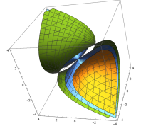
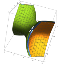
Figure 1: Representatives of the submanifolds in $\mathfrak{sl}^{*}(2)$ given by the surfaces with constant value of the Casimir for the Poisson structure in $\mathfrak{sl}^{*}(2)$ (left) and its deformation (right). Such submanifolds are symplectic submanifolds where the Poisson bivectors $\Lambda$ and $\Lambda_{z}$ admit a canonical form.

The splitting theorem on Poisson manifolds Va94 ensure that if $U_{p}$ is small enough, then there exist two different coordinate systems $\{x,y,C\}$ and $\{x_{z},y_{z},C_{z}\}$ where the Poisson bivectors related to $\{\cdot,\cdot\}$ and $\{\cdot,\cdot\}_{z}$ read $\Lambda=\partial_{x}\wedge\partial_{y}$ and $\Lambda_{z}=\partial_{x_{z}}\wedge\partial_{y_{z}}$. Hence, $C_{z}$ and $C$ are Casimir functions for $\Lambda_{z}$ and $\Lambda$, respectively. Moreover, $x_{z}=x_{z}(x,y,C),y_{z}=y_{z}(x,y,C),C_{z}=C_{z}(x,y,C)$. It follows from this that

$$\Phi:f(x_{z},y_{z},C_{z})\in C^{\infty}_{z}(U_{p})\mapsto f(x,y,C)\in C^{\infty}(U_{p})$$

is a Poisson algebra morphism.

If $\left\{v_{1},v_{2},v_{3}\right\}$ are the standard coordinates on $\mathfrak{sl}^{*}(2)$ and the relations (10) are satisfied, then $v_{i}=\xi_{i}(x_{z},y_{z},C_{z})$ holds for certain functions $\xi_{1},\xi_{2},\xi_{3}:\mathbb{R}^{3}\rightarrow\mathbb{R}$. Hence, the $\hat{v}_{z,i}=\xi_{i}(x,y,C)$ close the same commutation relations relative to $\{\cdot,\cdot\}$ as the $v_{i}$ do with respect to $\{\cdot,\cdot\}_{z}$. As $C$ is a Casimir invariant, the functions $v_{z,i}:=\xi_{i}(x,y,c)$, with a constant value of $c$, still close the same commutation relations among themselves as the $v_{i}$. Moreover, the functions $v_{z,i}$ become functionally dependent. Indeed,

$$C_{z}=C_{z}(v_{1},v_{2},v_{3})=C_{z}(\xi_{1}(x_{z},y_{z},C_{z}),\xi_{2}(x_{z},y_{z},C_{z}),\xi_{3}(x_{z},y_{z},C_{z})).$$

Hence, $c=C_{z}(\xi_{1}(x_{z},y_{z},c),\xi_{2}(x_{z},y_{z},c),\xi_{3}(x_{z},y_{z},c))$ and we conclude that $c=C_{z}(v_{z,1},v_{z,2},v_{z,3}).$

The previous argument allows us to recover the functions (16) in an algorithmic way. Actually, the functions $x_{z},y_{z},C_{z}$ and $x,y,C$ can be easily chosen to be

$$x_{z}:=v_{1},\qquad y_{z}:=-\frac{v_{2}}{{\,{\rm shc}}(2zv_{1})v_{1}},\qquad C_{z}:={\,{\rm shc}}(2zv_{1})v_{1}v_{3}-v_{2}^{2},$$

as well as

$$x=v_{1},\qquad y=-v_{2}/v_{1},\qquad C=v_{1}v_{3}-v_{2}^{2}.$$

Therefore,

$$\xi_{1}(x_{z},y_{z},C_{z})=x_{z},\qquad\xi_{2}(x_{z},y_{z},C_{z})=-y_{z}{\,{\rm shc}}(2zx_{z})x_{z},$$

$$\xi_{3}(x_{z},y_{z},C_{z})=\frac{C_{z}+x_{z}^{2}y_{z}^{2}{\,{\rm shc}}^{2}(2zx_{z})}{{\,{\rm shc}}(2zx_{z})x_{z}}.$$

Assuming that $C_{z}=c/4$, replacing $x_{z},y_{z}$ by $x=v_{1},y=-v_{2}/v_{1}$, respectively, and taking into account that $v_{z,i}:=\xi_{i}(x,y,c)$, one retrieves (16).

It is worth mentioning that due to the simple form of the Poisson bivectors in splitting form for three-dimensional Lie algebras, this method can be easily applied to such a type of Lie algebras.

Next, the above relations enable us to construct a Poisson algebra morphism

$$D_{z}:f(v_{1},v_{2},v_{3})\in C^{\infty}(\mathfrak{sl}_{z}^{*}(2))\mapsto D(f(v_{1,z},v_{2,z},v_{3,z}))\in C^{\infty}(M)$$

for every value of $z$ allowing us to pass the structure of the Poisson–Hopf algebra $C^{\infty}(\mathfrak{sl}_{z}^{*}(2))$ to $C^{\infty}(M)$. As a consequence, $D_{z}({C}_{z})$ satisfies the relations

$$\{D_{z}({C}_{z}),h_{z,i}\}_{\omega}=0,\qquad i=1,2,3.$$

Using the symplectic structure on $M$ and the functions $h_{z,i}$ written in terms of $\left\{h_{1},h_{2},h_{3}\right\}$, one can easily obtain the deformed vector fields ${\bf X}_{z,i}$ in terms of the vector fields ${\bf X}_{i}$. Finally, as ${\bf X}_{z,t}=\sum_{i=1}^{3}b_{i}(t){\bf X}_{z,i}$ holds, it is straightforward to verify that the brackets

$${\bf X}_{z,i}D(C_{z})=\{D(C_{z}),h_{z,i}\}=0,$$

imply that the function $D(C_{z})$ is a $t$-independent constant of the motion for each of the deformed LH system ${\bf X}_{z,t}$.

Consequently, deformations of LH-systems based on $\mathfrak{sl}(2)$ can be treated simultaneously, starting from their classical LH counterpart. The final result is summarized in the following statement.

Theorem 5.1

If $\phi:\mathfrak{sl}(2)\rightarrow C^{\infty}(M)$ is a morphism of Lie algebras with respect to the Lie bracket in $\mathfrak{sl}(2)$ and a Poisson bracket in $C^{\infty}(M)$, then for each $z\in\mathbb{R}$ there exists a Poisson algebra morphism $D_{z}:C^{\infty}(\mathfrak{sl}_{z}^{*}(2))\rightarrow C^{\infty}(M)$ such that for a basis $\{v_{1},v_{2},v_{3}\}$ satisfying the commutation relations (14) is given by

$$D_{z}(f(v_{1},v_{2},v_{3}))$$

$$=f\!\left(\!\phi(v_{1}),{\,{\rm shc}}(2z\phi(v_{1}))\phi(v_{2}),{\,{\rm shc}}(2z\phi(v_{1}))\frac{\phi^{2}(v_{2})}{\phi(v_{1})}+\frac{c}{4{\,{\rm shc}}(2z\phi(v_{1}))\phi(v_{1})}\right).$$

Provided that $h_{i}:=\phi(v_{i})$, the deformed Hamiltonian functions $h_{z,i}:=D_{z}(v_{i})$ adopt the form

$$h_{z,1}=h_{1},\qquad h_{z,2}={\,{\rm shc}}(2zh_{1})h_{2},$$

$$h_{z,3}={\,{\rm shc}}(2zh_{1})\frac{h_{2}^{2}}{h_{1}}+\frac{c}{4{\,{\rm shc}}(2zh_{1})h_{1}},$$

which satisfy the commutation relations (17).

The Hamiltonian vector fields ${\bf X}_{z,i}$ associated with $h_{z,i}$ through (5) turn out to be

$${\bf X}_{z,1}={\bf X}_{1},\qquad{\bf X}_{z,2}=\frac{h_{2}}{h_{1}}\bigl{(}\!{\,{\rm ch}(2zh_{1})}-{{\,{\rm shc}}(2zh_{1})}\bigr{)}{\bf X}_{1}+{\,{\rm shc}}(2zh_{1}){\bf X}_{2},$$

$${\bf X}_{z,3}=\left[\frac{h_{2}^{2}}{h_{1}^{2}}\bigl{(}{\rm ch}(2zh_{1})-2\,{\rm shc}(2zh_{1})\bigr{)}-\frac{c\;{\rm ch}(2zh_{1})}{4h_{1}^{2}{\rm shc}^{2}(2zh_{1})}\right]{\bf X}_{1}$$

$$\qquad\qquad\qquad+2\,\frac{h_{2}}{h_{1}}\,{\,{\rm shc}}(2zh_{1}){\bf X}_{2},$$

and satisfy the following commutation relations coming from (7)

$$[{\bf X}_{z,1},{\bf X}_{z,2}]={\rm ch}(2zh_{z,1}){\bf X}_{z,1},\qquad[{\bf X}_{z,1},{\bf X}_{z,3}]=2\,{\bf X}_{z,2},$$

$$[{\bf X}_{z,2},{\bf X}_{z,3}]={\rm ch}(2zh_{z,1}){\bf X}_{z,3}+4z^{2}{\rm shc}^{2}(2zh_{z,1})h_{z,1}h_{z,3}\,{\bf X}_{z,1}.$$

As a consequence, the deformed Poisson–Hopf system can be generically described in terms of the Vessiot–Guldberg Lie algebra corresponding to the non-deformed LH system as follows:

$${\bf X}_{z,t}=\sum_{i=1}^{3}b_{i}(t){\bf X}_{z,i}=\left[b_{1}(t)+b_{2}(t)\,\frac{h_{2}}{h_{1}}\bigl{(}\!{\,{\rm ch}(2zh_{1})}-{{\,{\rm shc}}(2zh_{1})}\bigr{)}\right]{\bf X}_{1}$$

$$\qquad\qquad\qquad+b_{3}(t)\left[\frac{h_{2}^{2}}{h_{1}^{2}}\bigl{(}{\rm ch}(2zh_{1})-2\,{\rm shc}(2zh_{1})\bigr{)}-\frac{c\;{\rm ch}(2zh_{1})}{4h_{1}^{2}{\rm shc}^{2}(2zh_{1})}\right]{\bf X}_{1}$$

$$\qquad\qquad\qquad+\,{\rm shc}(2zh_{1})\left(b_{2}(t)+2b_{3}(t)\frac{h_{2}}{h_{1}}\right){\bf X}_{2}.$$

This unified approach to nonequivalent deformations of LH systems possessing a common underlying Lie algebra suggests the following definition.

Definition 1

Let $(C^{\infty}(M),\{\cdot,\cdot\})$ be a Poisson algebra. A Poisson–Hopf Lie system is pair consisting of a Poisson–Hopf algebra $C^{\infty}(\mathfrak{g}_{z}^{*})$ and a $z$-parametrized family of Poisson algebra representations $D_{z}:C^{\infty}(\mathfrak{g}_{z}^{*})\rightarrow C^{\infty}(M)$ with $z\in\mathbb{R}$.

Next, constants of the motion for ${\bf X}_{z,t}$ can be deduced by applying the coalgebra approach introduced in BCHLS13Ham in the way briefly described in Section 3. In the deformed case, we consider the Poisson algebra morphisms

$$D_{z}:C^{\infty}\left(\mathfrak{sl}_{z}^{*}(2)\right)\rightarrow C^{\infty}(M),$$

$$D_{z}^{(2)}:C^{\infty}\left(\mathfrak{sl}_{z}^{*}(2)\right)\otimes C^{\infty}\left(\mathfrak{sl}_{z}^{*}(2)\right)\rightarrow C^{\infty}(M)\otimes C^{\infty}(M),$$

which by taking into account the coproduct (11) are defined by

$$D_{z}(v_{i}):=h_{z,i}({\bf x}_{1})\equiv h_{z,i}^{(1)},\quad i=1,2,3,$$

$$D_{z}^{(2)}\left({\Delta}_{z}(v_{1})\right)=h_{z,1}({\bf x}_{1})+h_{z,1}({\bf x}_{2})\equiv h_{z,1}^{(2)},$$

$$D_{z}^{(2)}\left({\Delta}_{z}(v_{k})\right)=h_{z,k}({\bf x}_{1}){\rm e}^{2zh_{z,1}({\bf x}_{2})}+{\rm e}^{-2zh_{z,1}({\bf x}_{1})}h_{z,k}({\bf x}_{2})\equiv h_{z,k}^{(2)},\quad k=2,3,$$

where ${\bf x}_{s}$ $(s=1,2)$ are global coordinates in $M$. We remark that, by construction, the functions $h_{z,i}^{(2)}$ satisfy the same Poisson brackets (17). Then $t$-independent constants of motion are given by (see (8))

$$F_{z}\equiv F_{z}^{(1)}:=D_{z}(C_{z}),\qquad F_{z}^{(2)}:=D_{z}^{(2)}\left({\Delta_{z}}(C_{z})\right),$$

where $C_{z}$ is the deformed Casimir (12). Explicilty, they read

$$F_{z}=\,{\rm shc}\!\left(2zh_{z,1}^{(1)}\right)h_{z,1}^{(1)}h_{z,3}^{(1)}-\left(h_{z,2}^{(1)}\right)^{2}=\frac{c}{4}\,,$$

$$F_{z}^{(2)}=\,{\rm shc}\!\left(2zh_{z,1}^{(2)}\right)h_{z,1}^{(2)}h_{z,3}^{(2)}-\left(h_{z,2}^{(2)}\right)^{2}.$$

6 The three classes of $\mathfrak{sl}(2)$ Lie–Hamilton systems on the plane and their deformation

We now apply Theorem 1 to the three classes of LH systems in the plane with a Vessiot–Guldberg Lie algebra isomorphic to $\mathfrak{sl}(2)$ according to the local classification performed in BBHLS , which was based in the results formerly given in GKO92 . Thus the manifold $M=\mathbb{R}^{2}$ and the coordinates $\mathbf{x}=(x,y)$. According to BBHLS ; BHLS , these three classes are named P₂, I₄ and I₅ and they correspond to a positive, negative and zero value of the Casimir constant $c$, respectively. Recall that these are non-diffeomorphic, so that there does not exist any local $t$-independent change of variables mapping one into another.

Table 1: The three classes of LH systems on the plane with underlying Vessiot–Guldberg Lie algebra isomorphic to $\mathfrak{sl}(2)$. For each class, it is displayed, in this order, a basis of vector fields ${\bf X}_{i}$, Hamiltonian functions $h_{i}$, symplectic form $\omega$, the constants of motion $F$ and $F^{(2)}$ as well as the corresponding specific LH systems.

$\bullet$ Class P2 with $c=4>0$

$\displaystyle{\quad{\bf X}_{1}=\frac{\partial}{\partial x}\qquad{\bf X}_{2}=x\frac{\partial}{\partial x}+y\frac{\partial}{\partial y}\qquad{\bf X}_{3}=(x^{2}-y^{2})\frac{\partial}{\partial x}+2xy\frac{\partial}{\partial y}}$

$\displaystyle{\quad h_{1}=-\frac{1}{y}\qquad h_{2}=-\frac{x}{y}\qquad h_{3}=-\frac{x^{2}+y^{2}}{y}\qquad\omega=\frac{{\rm d}x\wedge{\rm d}y}{y^{2}}}$

$\displaystyle{\quad F=1\qquad F^{\left(2\right)}=\frac{(x_{1}-x_{2})^{2}+(y_{1}+y_{2})^{2}}{y_{1}y_{2}}}$

– Complex Riccati equation

– Ermakov system, Milne–Pinney and Kummer–Schwarz equations with $c>0$

$\bullet$ Class I4 with $c=-1<0$

$\displaystyle{\quad{\bf X}_{1}=\frac{\partial}{\partial x}+\frac{\partial}{\partial y}\qquad{\bf X}_{2}=x\frac{\partial}{\partial x}+y\frac{\partial}{\partial y}\qquad{\bf X}_{3}=x^{2}\frac{\partial}{\partial x}+y^{2}\frac{\partial}{\partial y}}$

$\displaystyle{\quad h_{1}=\frac{1}{x-y}\qquad h_{2}=\frac{x+y}{2(x-y)}\qquad h_{3}=\frac{xy}{x-y}\qquad\omega=\frac{{\rm d}x\wedge{\rm d}y}{(x-y)^{2}}}$

$\displaystyle{\quad F=-\frac{1}{4}\qquad F^{(2)}=-\frac{(x_{2}-y_{1})(x_{1}-y_{2})}{(x_{1}-y_{1})(x_{2}-y_{2})}}$

– Split-complex Riccati equation

– Ermakov system, Milne–Pinney and Kummer–Schwarz equations with $c<0$

– Coupled Riccati equations

$\bullet$ Class I5 with $c=0$

$\displaystyle{\quad{\bf X}_{1}=\frac{\partial}{\partial x}\qquad{\bf X}_{2}=x\frac{\partial}{\partial x}+\frac{y}{2}\frac{\partial}{\partial y}\qquad{\bf X}_{3}=x^{2}\frac{\partial}{\partial x}+xy\frac{\partial}{\partial y}}$

$\displaystyle{\quad h_{1}=-\frac{1}{2y^{2}}\qquad h_{2}=-\frac{x}{2y^{2}}\qquad h_{3}=-\frac{x^{2}}{2y^{2}}\qquad\omega=\frac{{\rm d}x\wedge{\rm d}y}{y^{3}}}$

$\displaystyle{\quad F=0\qquad F^{\left(2\right)}=\frac{(x_{1}-x_{2})^{2}}{4y_{1}^{2}y_{2}^{2}}}$

– Dual-Study Riccati equation

– Ermakov system, Milne–Pinney and Kummer–Schwarz equations with $c=0$

– Harmonic oscillator

– Planar diffusion Riccati system

Table 2: Poisson–Hopf deformations of the three classes of $\mathfrak{sl}(2)$-LH systems written in Table 1. The symplectic form $\omega$ is the same given in Table 1 and $F\equiv F_{z}$.

$\bullet$ Class P2 with $c=4>0$

$\displaystyle{{\bf X}_{z,1}=\frac{\partial}{\partial x}\qquad{\bf X}_{z,2}=x\,\mathrm{ch}(2z/y)\frac{\partial}{\partial x}+y\,\mathrm{shc}(2z/y)\frac{\partial}{\partial y}}$

$\displaystyle{{\bf X}_{z,3}=\left(x^{2}-\frac{y^{2}}{\mathrm{shc}^{2}(2z/y)}\right)\mathrm{ch}(2z/y)\frac{\partial}{\partial x}+2xy\,\mathrm{shc}(2z/y)\frac{\partial}{\partial y}}$

$\displaystyle{{\bf h}_{z,1}=-\frac{1}{y}\qquad{\bf h}_{z,2}=-\frac{x}{y}\,\mathrm{shc}({2z}/{y})\qquad{\bf h}_{z,3}=-\frac{x^{2}\,\mathrm{shc}^{2}({2z}/{y})+y^{2}}{y\,\mathrm{shc}({2z}/{y})}}$

$\displaystyle{F_{z}^{(2)}=\frac{(x_{1}-x_{2})^{2}}{y_{1}y_{2}}\,\,{\rm shc}(2z/y_{1})\,{\rm shc}(2z/y_{2})\,{\rm e}^{2z\!/\!y_{1}}{\rm e}^{-2z\!/\!y_{2}}}$

$\displaystyle{\qquad\qquad\quad+\frac{(y_{1}+y_{2})^{2}}{y_{1}y_{2}}\,\frac{\,{\rm shc}^{2}(2z/y_{1}+2z/y_{2})}{\,{\rm shc}(2z/y_{1})\,{\rm shc}(2z/y_{2})}\,{\rm e}^{2z\!/\!y_{1}}{\rm e}^{-2z\!/\!y_{2}}}$

$\bullet$ Class I4 with $c=-1<0$

$\displaystyle{{\bf X}_{z,1}=\frac{\partial}{\partial x}+\frac{\partial}{\partial y}}$

$\displaystyle{{\bf X}_{z,2}=\frac{x+y}{2}\,\mathrm{ch}\!\left(\frac{2z}{x-y}\right)\left(\frac{\partial}{\partial x}+\frac{\partial}{\partial y}\right)+\frac{x-y}{2}\,\mathrm{shc}\!\left(\frac{2z}{x-y}\right)\left(\frac{\partial}{\partial x}-\frac{\partial}{\partial y}\right)}$

$\displaystyle{{\bf X}_{z,3}=\frac{1}{4}\,\mathrm{ch}\!\left(\frac{2z}{x-y}\right)\left[(x+y)^{2}+(x-y)^{2}\mathrm{shc}^{-2}\!\left(\frac{2z}{x-y}\right)\right]\left(\frac{\partial}{\partial x}+\frac{\partial}{\partial y}\right)}$

$\displaystyle{\qquad\qquad\quad+\frac{1}{2}\left(x-y\right)^{2}\mathrm{shc}\!\left(\frac{2z}{x-y}\right)\left(\frac{\partial}{\partial x}-\frac{\partial}{\partial y}\right)}$

$\displaystyle{{\bf h}_{z,1}=\frac{1}{x-y}\quad{\bf h}_{z,2}=\frac{(x+y)\,\mathrm{shc}\!\left(\frac{2z}{x-y}\right)}{2(x-y)}\quad{\bf h}_{z,3}=\frac{(x+y)^{2}\mathrm{shc}^{2}\!\left(\!\frac{2z}{x-y}\right)-(x-y)^{2}}{4(x-y)\,\mathrm{shc}\!\left(\!\frac{2z}{x-y}\right)}}$

$\displaystyle{F_{z}^{(2)}=\frac{(x_{1}-x_{2}+y_{1}-y_{2})^{2}}{4(x_{1}-y_{1})(x_{2}-y_{2})}\,\,{\rm shc}\!\left(\frac{2z}{x_{1}-y_{1}}\right)\,{\rm shc}\!\left(\frac{2z}{x_{2}-y_{2}}\right){\rm e}^{-\frac{2z}{x_{1}-y_{1}}}{\rm e}^{\frac{2z}{x_{2}-y_{2}}}}$

$\displaystyle{-\frac{(x_{1}+x_{2}-y_{1}-y_{2})\,{\rm shc}\!\left(\!\frac{2z}{x_{1}-y_{1}}+\frac{2z}{x_{2}-y_{2}}\right)}{4(x_{1}-y_{1})(x_{2}-y_{2})}\left[\frac{{\rm e}^{\frac{2z}{x_{2}-y_{2}}}(x_{1}-y_{1})}{\,{\rm shc}\bigl{(}\frac{2z}{x_{1}-y_{1}}\bigr{)}}+\frac{{\rm e}^{-\frac{2z}{x_{1}-y_{1}}}(x_{2}-y_{2})}{\,{\rm shc}\bigl{(}\frac{2z}{x_{2}-y_{2}}\bigr{)}}\right]}$

$\bullet$ Class I5 with $c=0$

$\displaystyle{{\bf X}_{z,1}=\frac{\partial}{\partial x}\qquad{\bf X}_{z,2}=x\,\mathrm{ch}\!\left({z}/{y^{2}}\right)\frac{\partial}{\partial x}+\frac{y}{2}\,\mathrm{shc}\!\left({z}/{y^{2}}\right)\frac{\partial}{\partial y}}$

$\displaystyle{{\bf X}_{z,3}=x^{2}\,\mathrm{ch}\!\left({z}/{y^{2}}\right)\frac{\partial}{\partial x}+xy\,\mathrm{shc}\!\left({z}/{y^{2}}\right)\frac{\partial}{\partial y}}$

$\displaystyle{{\bf h}_{z,1}=-\frac{1}{2y^{2}}\qquad{\bf h}_{z,2}=-\frac{x}{2y^{2}}\,\mathrm{shc}\!\left({z}/{y^{2}}\right)\qquad{\bf h}_{z,3}=-\frac{x^{2}}{2y^{2}}\,\mathrm{shc}\!\left({z}/{y^{2}}\right)}$

$\displaystyle{F_{z}^{(2)}=\frac{(x_{1}-x_{2})^{2}}{4y_{1}^{2}y_{2}^{2}}\,\,{\rm shc}\!\left(z/y_{1}^{2}\right)\,{\rm shc}\!\left(z/y_{2}^{2}\right){\rm e}^{z\!/\!y_{1}^{2}}{\rm e}^{-z\!/\!y_{2}^{2}}}$

Table 1 summarizes the three cases, covering vector fields, Hamiltonian functions, symplectic structure and $t$-independent constants of motion. The particular LH systems which are diffeormorphic within each class are also mentioned BHLS . Notice that for all of them it is satisfy the following commutation relations for the vector fields and Hamiltonian functions (the latter with respect to corresponding $\omega$):

$$[{\bf X}_{1},{\bf X}_{2}]={\bf X}_{1},\qquad[{\bf X}_{1},{\bf X}_{3}]=2{\bf X}_{2},\qquad[{\bf X}_{2},{\bf X}_{3}]={\bf X}_{3},$$

$$\{h_{1},h_{2}\}_{\omega}=-h_{1},\qquad\{h_{1},h_{3}\}_{\omega}=-2h_{2},\qquad\{h_{2},h_{3}\}_{\omega}=-h_{3}.$$

By applying Theorem 1 with the results of Table 1 we obtain the corresponding deformations which are displayed in Table 2. It is straightforward to verify that the classical limit $z\rightarrow 0$ in Table 2 recovers the corresponding starting LH systems and related structures of Table 1, in agreement with the relations (4) and (6).

7 A method to construct Lie–Hamilton systems

Section 5 showed that deformations of a LH system with a fixed LH algebra $\mathcal{H}_{\omega}\simeq\mathfrak{g}$ can be obtained through a Poisson algebra $C^{\infty}(\mathfrak{g}^{*})$, a given deformation and a certain Poisson morphism $D:C^{\infty}(\mathfrak{g}^{*})\rightarrow C^{\infty}(M)$. This section presents a simple method to obtain $D$ from an arbitrary $\mathfrak{g}^{*}$ onto a symplectic manifold $\mathbb{R}^{2n}$.

Theorem 7.1

Let $\mathfrak{g}$ be a Lie algebra whose Kostant–Kirillov–Souriau Poisson bracket admits a symplectic foliation in $\mathfrak{g}^{*}$ with a $2n$-dimensional $\mathcal{S}\subset\mathfrak{g}^{*}$. Then, there exists a LH algebra on the plane given by

$$\Phi:\mathfrak{g}\rightarrow C^{\infty}\bigl{(}\mathbb{R}^{2n}\bigr{)}$$

relative to the canonical Poisson bracket on the plane.

Proof

The Lie algebra $\mathfrak{g}$ gives rise to a Poisson structure on $\mathfrak{g}^{*}$ through the Kostant–Kirillov–Souriau bracket $\{\cdot,\cdot\}$. This induces a symplectic foliation on $\mathfrak{g}^{*}$, whose leaves are symplectic manifolds relative to the restriction of the Poisson bracket. Such leaves are characterized by means of the Casimir functions of the Poisson bracket. By assumption, one of these leaves is $2n$-dimensional. In such a case, the Darboux Theorem warrants that the Poisson bracket on each leave is locally symplectomorphic to the Poisson bracket of the canonical symplectic form on $\mathbb{R}^{2n}\simeq T^{*}\mathbb{R}^{n}$. In particular, there exists some Darboux coordinates mapping the Poisson bracket on such a leaf into the canonical symplectic bracket on $T^{*}\mathbb{R}^{n}$. The corresponding change of variables into the canonical form in Darboux coordinates can be understood as a local diffeomorphism $h:\mathcal{S}_{k}\rightarrow\mathbb{R}^{2n}$ mapping the Poisson bracket $\Lambda_{k}$ on the leaf $\mathcal{S}_{k}$ into the canonical Poisson bracket on $T^{*}\mathbb{R}^{n}$. Hence, $h$ gives rise to a canonical Poisson algebra morphism $\phi_{h}:C^{\infty}(\mathcal{S}_{k})\rightarrow C^{\infty}(T^{*}\mathbb{R}^{n})$.

As usual, a basis $\{v_{1},\ldots,v_{r}\}$ of $\mathfrak{g}$ can be considered as a coordinate system on $\mathfrak{g}^{*}$. In view of the definition of the Kostant–Kirillov–Souriau bracket, they span an $r$-dimensional Lie algebra. In fact, if $[v_{i},v_{j}]=\sum_{k=1}^{r}c_{ij}^{k}v_{k}$ for certain constants $c_{ij}^{k}$, then $\{v_{i},v_{j}\}=\sum_{k=1}^{r}c_{ij}^{k}v_{k}$. Since $\mathcal{S}_{k}$ is a symplectic submanifold, there is a local immersion $\iota:\mathcal{S}_{k}\hookrightarrow\mathfrak{g}^{*}$ which is a Poisson manifold morphism. In consequence,

$$\{\iota^{*}v_{i},\iota^{*}v_{j}\}=\sum_{k=1}^{r}c_{ij}^{k}\iota^{*}v_{k}.$$

Hence, the functions $\iota^{*}v_{i}$ span a finite-dimensional Lie algebra of functions on $\mathcal{S}$. Since $\mathcal{S}$ is $2n$-dimensional, there exists a local diffeomorphism $\phi:\mathcal{S}\rightarrow\mathbb{R}^{2n}$ and

$$\Phi:v\in\mathfrak{g}\mapsto\phi\circ\iota^{*}v\in C^{\infty}\bigl{(}\mathbb{R}^{2n}\bigr{)}$$

is a Lie algebra morphism.

Let us apply the above to explain the existence of three types of LH systems on the plane. We already know that the Lie algebra $\mathfrak{sl}(2)$ gives rise to a Poisson algebra in $C^{\infty}(\mathfrak{g}^{*})$. In the standard basis $v_{1},v_{2},v_{3}$ with commutation relations (14), the Casimir is (15). It turns out that the symplectic leaves of this Casimir are of three types:

• A one-sheet hyperboloid when $v_{1}v_{3}-v_{2}^{2}=k<0$.

• A conical surface when $v_{1}v_{3}-v_{2}^{2}=0$.

• A two-sheet hyperboloid when $v_{1}v_{3}-v_{2}^{2}=k>0$.

In each of the three cases we have the Poisson bivector

$$\Lambda=-v_{1}\frac{\partial}{\partial v_{1}}\wedge\frac{\partial}{\partial v_{2}}-2v_{2}\frac{\partial}{\partial v_{1}}\wedge\frac{\partial}{\partial v_{3}}-v_{3}\frac{\partial}{\partial v_{2}}\wedge\frac{\partial}{\partial v_{3}}.$$

Then, we have a changes of variables passing from the above form into Darboux coordinates

$$\bar{v}_{1}=v_{1},\qquad\bar{v}_{2}=-v_{2}/v_{1},\qquad C=v_{1}v_{3}-v_{2}^{2}.$$

Then,

$$v_{1}=v_{1},\qquad v_{2}=-\bar{v}_{1}\bar{v}_{2},\qquad v_{3}=(C+\bar{v}^{2}_{1}\bar{v}^{2}_{2})/\bar{v}_{1}.$$

On a symplectic leaf, the value of $C$ is constant, say $C=c/4$, and the restrictions of the previous functions to the leaf read

$$\iota^{*}v_{1}=v_{1},\qquad\iota^{*}v_{2}=-\bar{v}_{1}\bar{v}_{2},\qquad\iota^{*}v_{3}=c/(4\bar{v}_{1})+\bar{v}_{1}\bar{v}^{2}_{2}.$$

This can be viewed as a mapping $\Phi:\mathfrak{sl}(2)\rightarrow C^{\infty}(\mathbb{R}^{2})$ such that

$$\phi(v_{1})=x,\qquad\phi(v_{2})=-xy,\qquad\phi(v_{3})=c/(4x)+xy^{2},$$

which is obviously a Lie algebra morphism relative to the standard Poisson bracket in the plane. It is simple to proof that when $c$ is positive, negative or zero, one obtains three different types of Lie algebras of functions and their associated vector fields span the Lie algebras P₂, I₄ and I₅ as enunciated in BBHLS . Observe that since $\phi(v_{1})\phi(v_{3})-\phi(v_{2})^{2}=c/4$, there exists no change of variables on $\mathbb{R}^{2}$ mapping one set of variables into another for different values of $c$. Hence, Theorem 7.1 ultimately explains the real origin of all the $\mathfrak{sl}(2)$-LH systems on the plane.

It is known that $\mathfrak{su}(2)$ admits a unique Casimir, up to a proportional constant, and the symplectic leaves induced in $\mathfrak{su}^{*}(2)$ are spheres. The application of the previous method originates a unique Lie algebra representation, which gives rise to the unique LH system on the plane related to $\mathfrak{so}(3)$. All the remaining LH systems on the plane can be generated in a similar fashion. The deformations of such Lie algebras will generate all the possible deformations of LH systems on the plane.

8 Concluding remarks

It has been shown that Poisson–Hopf deformations of LH systems based on the simple Lie algebra $\mathfrak{sl}(2)$ can be formulated simultaneously by means of a geometrical argument, hence providing a generic description for the deformed Hamiltonian functions and vectors fields, starting from the corresponding classical counterpart. This allows for a direct determination of the deformed Hamiltonian functions and vector fields, as well as their corresponding Poisson brackets and commutators, by mere insertion of the data corresponding to the non-deformed LH system. This procedure has been explicitly illustrated by obtaining the deformed results of Table 2 from the classical ones of Table 1 through the application of Theorem 1.

Moreover we have explained a method to obtain (non-deformed) LH systems related to a LH algebra $\mathcal{H}_{\omega}$ by using the symplectic foliation in $\mathfrak{g}^{*}$, where $\mathfrak{g}$ is isomorphic to $\mathcal{H}_{\omega}$, which has been stated in Theorem 2. This result could further be applied in order to obtain deformations of LH systems beyond $\mathfrak{sl}(2)$. It is also left to accomplish the deformation of LH systems in other spaces of higher dimension.

It seems that the techniques provided here are potentially sufficient to provide a solution to the above mentioned problems. These will be the subject of further work currently in progress.

References

• (1) E. Abe, Hopf Algebras, Cambridge Tracts in Mathematics 74 (Cambridge: Cambridge Univ. Press, 1980)
• (2) A. Ballesteros, A. Blasco, F.J. Herranz, J de Lucas, C. Sardón, J. Differential Equations 258 (2015) 2873–2907
• (3) A. Ballesteros, A. Blasco, F.J. Herranz, F. Musso, O. Ragnisco, J. Phys.: Conf. Ser. 175 (2009) 012004
• (4) A. Ballesteros, R. Campoamor-Stursberg, E. Fernández-Saiz, F.J. Herranz, J. de Lucas, J. Phys. A: Math. Theor. 51 (2018) 065202
• (5) A. Ballesteros, J.F. Cariñena, F.J. Herranz, J. de Lucas, C. Sardón, J. Phys. A: Math. Theor. 46 (2013) 285203
• (6) A. Ballesteros, F.J. Herranz, J. Phys. A: Math. Gen. 29 (1996) L311–L316
• (7) A. Ballesteros, F.J. Herranz, O. Ragnisco, J. Phys. A: Math. Gen. 38 (2005) 7129–7144
• (8) A. Ballesteros, F.J. Herranz, M. del Olmo, M. Santander, J. Phys. A: Math. Gen. 28 (1995) 941–955
• (9) A. Ballesteros, O. Ragnisco, J. Phys. A: Math. Gen. 31 (1998) 3791–3813
• (10) A. Blasco A, F.J. Herranz, J. de Lucas, C. Sardón, J. Phys. A: Math. Theor. 48 (2015) 345202
• (11) R. Campoamor-Stursberg, J. Math. Phys. 57 (2016) 063508
• (12) J.F. Cariñena, J. Grabowski, J. de Lucas, J. Phys. A: Math. Theor. 43 (2010) 305201
• (13) J.F. Cariñena, J. Grabowski, G. Marmo, Lie–Scheffers Systems: a Geometric Approach (Bibliopolis, Naples, 2000)
• (14) J.F. Cariñena, J. Grabowski, G. Marmo, Rep. Math. Phys. 60 (2000) 237–258
• (15) J.F. Cariñena, A. Ibort, G. Marmo, G. Morandi, Geometry from Dynamics, Classical and Quantum (Springer, New York, 2015)
• (16) J.F. Cariñena, J. Lucas, Dissertations Math. (Rozprawy Mat.) 479 (2011) 1–162
• (17) J.F. Cariñena, J. de Lucas, C. Sardón, Int. J. Geom. Methods Mod. Phys. 10 (2013) 1350047
• (18) V. Chari, A. Pressley, A Guide to Quantum Groups (Cambridge Univ. Press, Cambridge, 1994)
• (19) A. González-López, N. Kamran, P.J. Olver, Proc. London Math. Soc. 64 (1992) 339–368
• (20) N.H. Ibragimov, A.A. Gainetdinova, Int. J. Non-linear Mech. 90 (2017) 50–71
• (21) A. Inselberg, On classification and superposition principles for nonlinear operators, Thesis (Ph.D.), University of Illinois at Urbana-Champaign, ProQuest LLC, Ann Arbor, MI, 1965
• (22) A. Inselberg, J. Math. Anal. Appl. 40 (1972) 494–508
• (23) S. Lie, Vorlesungen über continuirliche Gruppen mit geometrischen und anderen Anwendungen (B. G. Teubner, Leipzig, 1893)
• (24) S. Majid, Foundations of Quantum Group Theory (Cambridge Univ. Press, Cambridge, 1995)
• (25) Ch. Ohn, Lett. Math. Phys. 25 (1992) 85–88
• (26) L.V. Ovsiannikov, Group Analysis of Differential Equations (Academic Press, New York, 1982)
• (27) R.S. Palais, A Global Formulation of the Lie Theory of Transformation Groups (AMS, Providence RI, 1957)
• (28) S. Shnider, P. Winternitz, Lett. Math. Phys. 8 (1984) 69–78
• (29) I. Vaisman, Lectures on the Geometry of Poisson manifolds (Birkhäuser Verlag, Basel, 1994)
• (30) V.S. Varadarajan, Lie groups, Lie algebras, and their Representations, Graduate Texts in Mathematics 102 (Springer-Verlag, New York, 1984)
• (31) E. Vessiot, Ann. Sci. de l’École Norm. Sup. (3) 9 (1892) 197–280
• (32) P. Winternitz, in Nonlinear phenomena, ed. by K.B. Wolf, Lectures Notes in Physics vol. 189, (Springer, New York, 1983), pp. 263–331