Ordered array of $\omega$ particles in $\beta$-Ti matrix studied by small-angle x-ray scattering

Abstract

Nano-sized particles of $\omega$ phase in a $\beta$-Ti alloy were investigated by small-angle x-ray scattering using synchrotron radiation. We demonstrated that the particles are spontaneously weakly ordered in a three-dimensional cubic array along the $\langle 100\rangle$-directions in the $\beta$-Ti matrix. The small-angle scattering data fit well to a three-dimensional short-range-order model; from the fit we determined the evolution of the mean particle size and mean distance between particles during ageing. The self-ordering of the particles is explained by elastic interaction between the particles, since the relative positions of the particles coincide with local minima of the interaction energy. We performed numerical Monte-Carlo simulation of the particle ordering and we obtained a good agreement with the experimental data.

1 Introduction

Metastable $\beta$-Ti alloys are increasingly used in aerospace and automotive industry mainly due to excellent corrosion resistance and high specific strength. The high strength is achieved through ageing treatment involving several phase transformations [1]. Therefore, investigation of these phase transformations is of significant importance.

Above 883${\mkern 4.0mu{}^{\circ}\mkern-2.0mu\rm C}$, pure titanium crystallizes in a body-centered cubic structure ($\beta$ phase). When cooled below this temperature ($\beta$-transus) it martensitically transforms to a hexagonal close-packed structure ($\alpha$ phase). Metastable $\beta$-Ti alloys contain a sufficient amount of $\beta$-stabilizing elements (Mo, V, Nb, Fe) so that the martensitic $\beta\rightarrow\alpha$ transformation is suppressed and the $\beta$ phase is retained after quenching to room temperature [2].

Several metastable phases can emerge during ageing of these alloys depending on the content of $\beta$-stabilizing elements. The present study focuses on hexagonal $\omega$ phase. Tiny and uniformly distributed particles of the $\omega$ phase serve as precursors for a subsequent precipitation of the $\alpha$-phase particles that are responsible for significant strengthening.

The $\omega$ phase is formed upon quenching by a diffusionless displacive transformation as first proposed by Hatt et al. [3] and lucidly described by de Fontaine [4]. The transformation can be described as a collapse of two neighbouring (111)_β planes into one plane. More formally, these two planes are displaced by $\pm\frac{1}{12}\left[111\right]$ along the body diagonal of the cubic unit cell. One (111)_β plane between two pairs of collapsed planes remains unchanged. This produces a hexagonal structure with two differently populated alternating ’basal’ planes. Such hexagonal structure is coherent with the parent $\beta$ phase [5]. It was shown experimentally that this displacive $\beta\rightarrow\omega$ transformation is completely reversible at low temperatures at which diffusion does not play a role [6]. The $\omega$ phase forms fine, a few nanometers large particles uniformly dispersed throughout the $\beta$ matrix. Due to its formation mechanism, the $\omega$ phase can exist only in certain orientations with respect to the $\beta$ matrix. The topotactical relationship between the $\beta$ and $\omega$ lattices can be described as [7]

$$(0001)_{\omega}\parallel(111)_{\beta},\ \left[11\bar{2}0\right]{}_{\omega}\parallel[011]_{\beta}.$$ (1)

The particles of the $\omega$ phase further evolve and grow during ageing through a diffusion controlled reaction [8]. This process is irreversible and is accompanied by rejection of $\beta$ stabilizing elements from the $\omega$ phase.

It has been observed that the shape of the $\omega$ particles can be either ellipsoidal or cuboidal. According to Blackburn et al. [9], the shape is related to the lattice misfit strain. They suggested that the ellipsoidal shape of the $\omega$ precipitates arises from an anisotropy of the strain energy of the precipitate rather than the matrix, whereas the cuboidal shape is determined by the strain energy in the matrix.

Despite countless studies describing the $\omega$ phase, there is still not much known about the causes of formation of the $\omega$-phase particles and their spatial ordering. Some argue that the $\omega$ particles formation follows from a spinodal chemical separation of the $\beta$ phase [10, 11]. This conclusion is based on observations of the spatial ordering and/or chemical inhomogeneity of the particles and the host material. Others suggest that the formation of these particles can be attributed to elastic instabilities of the parent $\beta$ matrix [12].

In the last decades, kinetics of the phase separation in alloys has been intensively studied both theoretically and by various experimental methods. For the theoretical description of the phase separation both macroscopic and microscopic approaches have been published, the former describes the phases as elastic continua divided by ideally sharp interfaces, the latter takes into account movement of individual atoms. The description is based on classical works of Cahn and Hilliard [13, 14] and Lifshitz, Slyozov and Wagner [15, 16] (LSW theory) and includes various processes denoted spinodal decomposition, coarsening or Ostwald ripening (see also the review in [17]). From numerous numerical simulations and experimental data it follows that the time-dependent structure function

$$S(Q,t)=\left\langle\left|\int{\rm d}^{3}{\bm{r}}c({\bm{r}}){\rm e}^{-{\rm i}{\bm{Q}}.{\bm{r}}}\right|^{2}\right\rangle,$$ (2)

i.e., the square of the modulus of the Fourier transformation of the concentration function $c({\bm{r}})$ of a given phase averaged over a statistical ensemble, obeys a universal scaling law [18]

$$S(Q,t)\sim Q_{\rm max}(t)^{-3}F(Q/Q_{\rm max}(t)),$$ (3)

where $Q_{\rm max}(t)$ is the position of the maximum of the structure function $S(Q,t)$ and $F$ is a time-independent universal function. From the time-dependence of $Q_{\rm max}$ we can deduce the evolution of the characteristic length $L(t)\sim 2\pi/Q_{\rm max}(t)$ during the coarsening process; from the LSW theory the asymptotic behavior $Q_{\rm max}(t)^{-3}\sim A+Bt$ follows.

$\omega$ phase particles in metastable $\beta$-Ti alloys are nanometers in size and after ageing have slightly different electron density than the parent $\beta$ matrix (i.e. the x-ray indexes of refraction of the particles and the matrix are different). Small-angle x-ray scattering (SAXS) is an ideal technique to determine the structure function, since the reciprocal-space distribution of the scattered intensity is proportional to the structure function multiplied by the square of the difference in the electron densities of the $\beta$ and $\omega$ phases. SAXS is a nondestructive technique based on elastic scattering from electron density inhomogeneities within the sample. The SAXS instrument records scattered intensity at small scattering angles, i.e., close to the direction of the incident beam. Obtained SAXS data contain information about important microstructural parameters such as size, shape, volume and space correlations of the scatterers [19].

To our knowledge, only a limited number of experiments employing SAXS on $\omega$ particles in titanium alloys has been performed and published. Fratzl et al. [20] investigated the growth of $\omega$-phase particles in single crystals of Ti–20 at.%Mo. They found that the radii of the $\omega$ particles increased with ageing time as $\sim t^{1/3}$ and then stabilized at the value of approximately 75Å. The same group of authors later investigated $\omega$ and $\alpha$ phase precipitation in Ti–12 at.%Mo single crystals by the means of SAXS [21]. In their work, the authors determined the shape of the $\omega$ particles and then observed the nucleation and coarsening of $\alpha$ plates which destroyed the $\omega$ structure.

In our previous paper [22] we studied the structure of the $\omega$ particles in a single-crystalline $\beta$ matrix by x-ray diffraction (XRD). We confirmed the validity of the topotactical relations in Eq. (1) and found that the $\beta$ lattice is locally compressed around the particles. In this paper we perform a systematic SAXS study of the evolution of sizes of the $\omega$ particles in single-crystalline $\beta$-Ti alloy samples during ageing. We demonstrate that the $\omega$ particles are self-ordered and create a three-dimensional cubic array along the crystallographic axes $\langle 100\rangle_{\beta}$ of the $\beta$ matrix and that the mean distance between the particles is proportional to their mean size. We explain the ordering mechanism by considering the energy of the elastic interaction between the particles caused by the local deformation of the lattice. Finally, we compare the measured data with the scaling behavior in Eq. (3).

The paper is written as follows. The next section contains a brief description of the growth of the Ti-alloy single crystals and the SAXS experiments. Section 3 contains a phenomenological model of the arrays of particles that makes it possible to fit the experimental data and to determine basic structural parameters. The results of the SRO model are also presented in Section 3. The driving force of the self-ordering process is discussed in Section 4. The Section 5 provides a discussion of the obtained results.

2 Experiments

Single crystals of one of the metastable $\beta$ titanium alloys, TIMETAL LCB were grown in a commercial optical floating zone furnace (model FZ-T-4000-VPM-PC, Crystal Systems Corp., Japan) with four 1000 W halogen lamps. The growth process was carried out in a protective Ar atmosphere with Ar flow of 0.25 l/min and pressure of 2.5 bar. The growth speed was 10 mm/h. The grown ingots had roughly circular cross section with diameter in the range of 8 – 10 mm. The length of the single crystals was typically around 9cm. The details of the single crystal growth process and characterization of the resulting ingot can be found elsewhere [23]. During single crystal growth, a shift in chemical composition of the material is possible. In order to assess this change, concentrations of individual elements were determined both for precursor material and grown ingot. Two experimental methods were used. Concentrations of the main alloying elements (Ti, Mo, Fe, Al) were determined by energy dispersive x-ray spectroscopy (EDX) using scanning electron microscope FEIQuanta200FEG. Because titanium alloys are prone to contamination by interstitial N and O, the concentrations of these elements were checked by an automatic analyzer LECOTC500C. The chemical composition of the precursor and resulting single crystal are summarized in Tab. 1.

sample	Ti	Mo	Fe	Al	N	O
precursor	$88.7\pm 0.7$	$4.1\pm 0.4$	$3.7\pm 0.5$	$3.1\pm 0.2$	$0.011\pm 0.004$	$0.40\pm 0.06$
crystal	$88.4\pm 0.4$	$4.3\pm 0.3$	$3.4\pm 0.4$	$3.1\pm 0.2$	$0.29\pm 0.03$	$0.55\pm 0.06$

Table 1: Chemical composition of the precursor material and the resulting single crystal in at. %

Each crystal was solution treated at 860${\mkern 4.0mu{}^{\circ}\mkern-2.0mu\rm C}$ for 4h in an evacuated quartz tube and water quenched in order to homogenize the structure and ensure the retention of $\beta$ phase. Subsequently, the crystals were cut into 1.2mm thick slices perpendicular to the length of the crystal. The slices were then aged in salt bath at three temperatures 300${\mkern 4.0mu{}^{\circ}\mkern-2.0mu\rm C}$, 335${\mkern 4.0mu{}^{\circ}\mkern-2.0mu\rm C}$, and 370${\mkern 4.0mu{}^{\circ}\mkern-2.0mu\rm C}$ for 2, 4, 8, 16, 32, 64, 128 and 256h. At these ageing temperatures, the $\omega$ phase particles grow, but at least at the lowest temperatures in the series, the precipitation of the $\alpha$-Ti phase is not expected [24, 25]. The samples were then ground and polished from both sides utilizing 500, 800, 1200, 2400 and 4000 grit SiC papers. Final polishing was carried out on a vibratory polisher using 0.3$\mu$m and 0.05$\mu$m aqueous alumina (Al₂O₃) suspensions and 0.05$\mu$m colloidal silica. The final thickness of the samples for SAXS measurement was approximately 200$\mu$m. The crystallographic orientation of the slices was determined by standard Laue diffraction with the accuracy better than 1deg.

Small-angle x-ray scattering (SAXS) experiments have been carried out at the beamline 15-ID at APS, Argonne National Laboratory (USA). We used the photon energy of 25keV, the width of the primary x-ray beam was set to $150\times 150$$\mu$m. The scattered beam was detected by a large two-dimensional detector with $2048\times 2048$ pixels. One measurement took 60s and we took five SAXS pictures for different areas of each sample. The samples were mounted on a goniometer head allowing for a precise alignment of the crystallographic axes of the sample lattice with respect to the primary x-ray beam. For each ageing temperature we obtained the SAXS patterns in three directions $[001]_{\beta},\ [110]_{\beta}$ and $[111]_{\beta}$ of the primary beam with respect to the $\beta$-Ti lattice. The SAXS data were calibrated by a standard procedure [19], using Ag-behenate and glassy carbon samples for angular and intensity calibrations, respectively. After the calibration, the scattered intensities were expressed as photon fluxes scattered from unit sample volume into unit solid angle of one sr normalized to unit flux density of the primary radiation and corrected to the sample absorption.

In figure 1 we plotted the SAXS intensity maps of the samples after various ageing times (ageing temperature 300${\mkern 4.0mu{}^{\circ}\mkern-2.0mu\rm C}$) measured in the orientation $[001]_{\beta}$ of the primary x-ray beam. The arrow denotes the orientation of the $[100]_{\beta}$ direction in the host lattice determined by independent x-ray diffraction (the Laue method). The maps clearly exhibit side maxima in directions $[100]_{\beta},\ [010]_{\beta}$ indicating that the particles are arranged in a disordered three-dimensional cubic array with the axes along $\langle 100\rangle_{\beta}$. With increasing ageing time the side maxima move closer to the origin and they become stronger and narrower; this development can be explained by increasing mean distance $L_{0}$ of the neighboring particles and increasing particle size. Figure 2 shows the SAXS maps of the sample after 300${\mkern 4.0mu{}^{\circ}\mkern-2.0mu\rm C}$/256h ageing measured for the three crystallographic orientations of the primary beam; the positions of the side maxima again support the hypothesis of the ordering of the particles along $\langle 100\rangle_{\beta}$ axes.

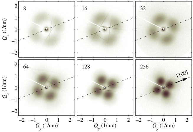
Figure 1: The SAXS maps of samples after ageing at 300${\mkern 4.0mu{}^{\circ}\mkern-2.0mu\rm C}$; the time of ageing in hours is indicated in the upper left corners of the panels. The measurements have been carried out in the $[001]_{\beta}$-orientation of the primary x-ray beam. The line scans plotted in Figure 5 were extracted from these maps along the dashed lines.

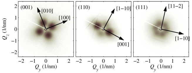
Figure 2: The SAXS maps of the sample after 300${\mkern 4.0mu{}^{\circ}\mkern-2.0mu\rm C}$/256h ageing measured in three orientations of the primary x-ray beam. The arrows denote the crystallographic directions in the $\beta$ host lattice determined by the Laue method.

The SAXS intensity maps of samples aged at 335${\mkern 4.0mu{}^{\circ}\mkern-2.0mu\rm C}$ are quite similar to Fig. 1, therefore, we do not present them here. In Fig. 3 we show the maps of the samples aged at 370${\mkern 4.0mu{}^{\circ}\mkern-2.0mu\rm C}$, since their appearance obviously differs from figure 1.

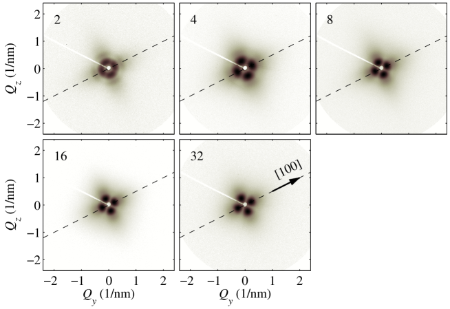
Figure 3: The same situation as in Figure 1, ageing temperature 370${\mkern 4.0mu{}^{\circ}\mkern-2.0mu\rm C}$.

Theoretical description of the small-angle x-ray scattering from an ordered three-dimensional array of particles along with numerical simulation and fitting to the experimental data will be described in the next section.

3 Short-range-order model of the ordering of particles

In this section we present a model for the simulation and fitting of the SAXS data. The model is purely phenomenological, but its simplicity makes it possible to fit numerically the measured data. A more physically substantiated simulation approach will be presented in Sect. 4.

The signal measured in a small-angle-scattering experiment (SAXS) in a given pixel of a two-dimensional detector

$$J=I_{\rm inc}\frac{{\rm d}\sigma}{{\rm d}\Omega}\Delta\Omega$$ (4)

is proportional to the intensity of the primary beam $I_{\rm inc}$, the solid angle $\Delta\Omega$ determined by the angular aperture of the detector pixel and the differential cross-section ${\rm d}\sigma/{\rm d}\Omega$ of the scattering process.

The differential scattering cross-section is simulated using a standard approach [26] including the kinematical approximation (i.e. neglecting multiple scattering from the particles) and the far-field limit. The explicit formula for the differential scattering cross-section reads:

$$\frac{{\rm d}\sigma}{{\rm d}\Omega}=\frac{K^{4}}{4\pi^{2}}|\Delta n|^{2}{\rm e}^{-\mu T}\left\langle\sum_{n}\sum_{m}\Omega_{n}^{\rm FT}({\bm{Q}})\Omega_{m}^{{\rm FT}*}({\bm{Q}}){\rm e}^{-{\rm i}{\bm{Q}}.({\bm{r}}_{n}-{\bm{r}}_{m})}\right\rangle.$$ (5)

Here we denoted $K=2\pi/\lambda$, $\mu$ is the linear absorption coefficient, $T$ is the sample thickness measured along the primary x-ray beam, and $\Delta n$ is the difference of the refraction indexes of the particle and the host material (caused by a slight difference in their chemical compositions). It is therefore assumed that the refraction index (which is proportional to the electron density) is homogeneous within the particle and also the electron density of the host material is assumed homogeneous. The electron density is determined by chemical composition (i.e. concentration of impurity atoms Mo, Fe and Al), as well as by the specific volume per one atom, which is affected by elastic deformation of the lattice and/or by the presence of structure defects. $\Omega_{n}^{\rm FT}(\bm{Q})$ is the Fourier transformation of the shape function of the $n$-th particle:

$$\Omega_{n}^{\rm FT}({\bm{Q}})=\int{\rm d}^{3}{\bm{r}}\Omega_{n}({\bm{r}}){\rm e}^{-{\rm i}{\bm{Q}}.{\bm{r}}};$$

the shape function $\Omega_{n}({\bm{r}})$ is unity inside and zero outside the particle. Further, ${\bm{r}}_{n}$ in Eq. (5) is the position vector of the $n$-th particle, the double sum $\sum_{n}\sum_{m}$ runs over all particles in the irradiated sample volume, and the averaging $\langle\ \rangle$ is performed over random positions and sizes of the particles. The scattering vector ${\bm{Q}}={\bm{K}}_{f}-{\bm{K}}_{i}$ is considered in vacuum, since the refraction correction is unimportant in our transmission geometry and the absorption effect is included in the absorption term $\exp(-\mu T)$ in Eq. (5). It is worthy to note that the measured signal in Eqs. (4,5) is proportional to the structure function defined in Eq. 2:

$$J=I_{\rm inc}|\Delta n|^{2}\frac{K^{4}}{4\pi^{2}Q_{\rm max}^{3}}F\left(\frac{{\bm{Q}}}{Q_{\rm max}}\right)\Delta\Omega,$$ (6)

where $F$ is the universal scaling function from Eq. (3).

In the literature, several models can be found describing a possible correlation of the particle sizes with their positions [26]. In the following we assume the local-monodisperse approximation (LMA). Using this approach, the irradiated sample volume consists of many domains, one domain contains particles of a given size and given mean distance between nearest particles. The differential scattering cross-section is then

$$\frac{{\rm d}\sigma}{{\rm d}\Omega}=\frac{K^{4}}{4\pi^{2}}|\Delta n|^{2}\left\langle\left|\Omega_{R}^{\rm FT}({\bm{Q}})\right|^{2}G_{R}({\bm{Q}})\right\rangle_{\rm sizes},$$ (7)

here we have denoted

$$G_{R}({\bm{Q}})=\left\langle\sum_{n}\sum_{m}{\rm e}^{-{\rm i}{\bm{Q}}.({\bm{r}}_{n}-{\bm{r}}_{m})}\right\rangle_{\rm positions}$$ (8)

the correlation function of the positions of the particles with a given radius $R$. In the following we omit the subscript $R$ for simplicity.

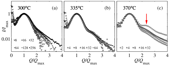
Figure 4: Line scans across the satellite maxima measured on samples after ageing at 300${\mkern 4.0mu{}^{\circ}\mkern-2.0mu\rm C}$ (a), 335${\mkern 4.0mu{}^{\circ}\mkern-2.0mu\rm C}$ (b), and 370${\mkern 4.0mu{}^{\circ}\mkern-2.0mu\rm C}$ (c). The scans are normalized to the same height and position of the first satellite maximum. The red arrow in panel (c) denotes the position of the secondary satellite maximum.

Since the position of a particle is only affected by the positions of the particles in few nearest coordination shells, the ordering of the particles can be described by a short-range order model (SRO). In this model we assume that the distances of a given particle from their neighbors are random with a given statistical distribution. As the $\omega$ particles create a cubic array, the three-dimensional correlation function $G({\bm{Q}})$ can be expressed as a direct product of three one-dimensional correlation functions as shown by Eads et al. [27]. The one-dimensional correlation function $G^{(1)}({\bm{Q}})$ can be calculated directly [27, 28]:

$$G^{(1)}({\bm{Q}})=N\left\{1+2{\rm Re}\left[\frac{\xi({\bm{Q}})}{1-\xi({\bm{Q}})}\left(N-\frac{(\xi({\bm{Q}}))^{N}-1}{\xi({\bm{Q}})-1}\right)\right]\right\}.$$ (9)

Here we denoted $N$ the number of coherently irradiated particles in one dimension and

$$\xi({\bm{Q}})=\left\langle{\rm e}^{-{\rm i}{\bm{Q}}.{\bm{L}}}\right\rangle,$$

where ${\bm{L}}$ is the random vector connecting the actual centers of neighboring particles lying in the same one-dimensional chain. In the following we assume that $N$ is very large and we use the limiting expression for $G^{(1)}({\bm{Q}})$:

$$G^{(1)}({\bm{Q}})\rightarrow N\left[1+2{\rm Re}\left(\frac{\xi({\bm{Q}})}{1-\xi({\bm{Q}})}\right)\right].$$

The three-dimensional correlation function $G({\bm{Q}})$ can be expressed as a product of three one-dimensional correlation functions along the orthogonal axes parallel to the axes of the cubic array of particles. Since the coordinate $Q$ of the intensity line scans in Fig. 4 is parallel to the array axis and the other two coordinates along the scans are approximately zero (we neglect the curvature of the Ewald sphere), the correlation function used for the simulation of the line scans is

$$G(Q,0,0)=N_{\parallel}N_{\bot}^{2}\left(\frac{\sigma_{L}}{L_{0}}\right)^{4}\left[1+2{\rm Re}\left(\frac{\xi({\bm{Q}})}{1-\xi({\bm{Q}})}\right)\right],$$ (10)

where we used the limiting value $N(\sigma_{L}/L_{0})^{2}$ of the one-dimensional correlation function for the zero argument. $N_{\parallel}$ and $N_{\bot}$ denote the numbers of the coherently irradiated particles in the directions parallel and perpendicular to the primary beam, respectively. $L_{0}$ is the mean inter-particle distance and $\sigma_{L}$ is its root-mean square (rms) deviation. The total number of the coherently irradiated particles can be expressed by the irradiated sample volume $V$:

$$N_{\parallel}N_{\bot}^{2}=\frac{V}{L_{0}}.$$

In the simulation we assume that the particles are spherical, and calculating the function $\xi({\bm{Q}})$, we apply the condition that neighboring particles must not intersect. Therefore, in the averaging over all possible ${\bm{L}}$’s we excluded the case $|{\bm{L}}|<2R$, where $R$ is a random particle radius (assumed fixed in the averaging over ${\bm{L}}$’s). Therefore, we assumed a truncated normal distribution of the random vectors ${\bm{L}}$ with the mean value ${L}_{0}=\langle|{\bm{L}}|\rangle$ and rms deviation $\sigma_{L}$. Further, we assumed the Gamma distribution of the particle radii $R$ with the mean value $R_{0}$ and the rms dispersion $\sigma_{R}$; for each radius we considered the correlation function calculated by Eq. (9) assuming the mean particle distance $L_{0}$ proportional to the actual value of $R$: $L_{0}=\zeta R$. The averaging in Eq. (7) is then performed numerically by integrating over $R$-values, keeping $\zeta$ constant. It can be proved by a direct calculation that the short-range order model presented here obeys the scaling law in Eq. (3), if the mean values $R_{0}$ and $L_{0}$ are proportional ($L_{0}=\zeta R_{0}$) and the relative rms deviations are constant, i.e. $\sigma_{L}\sim L_{0}$ and $\sigma_{R}\sim R_{0}$.

We have checked the validity of the scaling law in Eq. (3) by rescaling the line scan to the same position and height of the satellite maxima, the results are displayed in figure 4. From the figure it follows that at the two lower ageing temperatures the line scans are scaled according to Eq. (3) (panels a and b). The large spread of intensity values for higher ${\bm{Q}}$ in Fig. 4 is due to high noise due to background subtraction. However, obvious deviations from the scaling behavior can be observed for the highest ageing temperature of 370${\mkern 4.0mu{}^{\circ}\mkern-2.0mu\rm C}$, see Fig. 4(c). In particular, the line scan of the sample after 2h ageing exhibits secondary side maximum (denoted by arrow), which indicates a better ordering of the particle positions and/or smaller rms deviation of the particle sizes. We do not observe this secondary maximum for longer ageing times for the other temperatures. The secondary maximum gradually disappears during annealing.

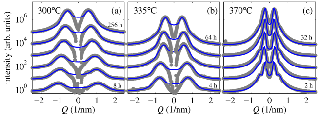
Figure 5: The line scans extracted from the SAXS maps (grey dots) for samples aged at 300${\mkern 4.0mu{}^{\circ}\mkern-2.0mu\rm C}$ (a), 335${\mkern 4.0mu{}^{\circ}\mkern-2.0mu\rm C}$ (b) and 370${\mkern 4.0mu{}^{\circ}\mkern-2.0mu\rm C}$ (c) and their fits by the SRO model (lines). The numbers denote the ageing time, the scans are shifted vertically for clarity.

From the SAXS maps we extracted line scans along the $[100]_{\beta}$ direction (dashed lines in figures 1 and 3) and fitted them with SRO model. Formulas in Eqs. (7, 9, 10) yield absolute flux densities therefore from the fit we were able to determine the contrast $|\Delta n|$ in the refraction indexes of the particle material and the host phase, appearing in the multiplicative pre-factor. Nevertheless, in order to determine both $|\Delta n|$ and the mean particle sizes, we had to assume that the mean inter-particle distance $L_{0}$ and the mean radius $R_{0}$ are proportional, i.e., $L_{0}=\zeta R_{0}$, and the proportional factor $\zeta$ is the same in all samples in the same ageing series.

Figure 5 compares the measured (grey points) and fitted (lines) line scans. It is obvious that the agreement of the theory with experimental data is quite good. Figure 6 shows the measured and fitted line scans of the sample after 300${\mkern 4.0mu{}^{\circ}\mkern-2.0mu\rm C}$/8h ageing in more detail; we plotted by dotted and dashed lines the contributions of the particle shape (function $\langle\left|\Omega^{\rm FT}({\bm{Q}})\right|^{2}\rangle$) and the correlation function $G({\bm{Q}})$ of the particle positions, respectively. From the figure it is obvious that the shape factor slightly shifts the side maxima at $Q_{\rm max}$ towards smaller $|Q|$ so that it would be misleading to determine the mean particle distance $L_{0}$ just from the formula $L_{0}=2\pi/Q_{\rm max}$.

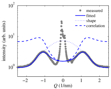
Figure 6: The line scan extracted from the SAXS map of sample after 300${\mkern 4.0mu{}^{\circ}\mkern-2.0mu\rm C}$/8h ageing (points) and its fit by the SRO model (full line). The contributions of the particle shape and correlation to the simulated line scan are displayed by dotted and dashed lines, respectively.

Parameters of the particle ordering determined from the fits of the line scans are summarized in Fig. 7. In panel (a) we plotted the time-dependence of the mean particle radius $R$ determined from the SAXS data. In this panel, we compare these radii with the particle radii determined by XRD using the method described in our previous paper [22]. For the sample series aged at 300${\mkern 4.0mu{}^{\circ}\mkern-2.0mu\rm C}$ and 335${\mkern 4.0mu{}^{\circ}\mkern-2.0mu\rm C}$ both radii coincide within the error limits and their time-dependence roughly agrees with the prediction of the LSW theory $[R_{0}(t)]^{3}\sim A+Bt$ ($A$ and $B$ are constants). The third series aged at 370${\mkern 4.0mu{}^{\circ}\mkern-2.0mu\rm C}$ behaves in a different way. With increasing ageing time the particle radii determined from XRD decrease, however, the error bars of these radii are larger than for the other ageing temperatures. In order to obtain a reasonably good fit of the data from the third sample series, we had to fit the parameters $L_{0}$ and $R_{0}$ independently, not considering the proportionality factor $\zeta$. This fact makes the fitting results less reliable than for the other two series, however, it is obvious that the particles sizes determined from SAXS are larger than those from XRD. Figure 7(b) displays the time dependence of the mean particle distance $L_{0}$ determined from SAXS. Again, for sample series at 300${\mkern 4.0mu{}^{\circ}\mkern-2.0mu\rm C}$ and 335${\mkern 4.0mu{}^{\circ}\mkern-2.0mu\rm C}$ $L_{0}$ increases with the ageing time and follows the polynomial formula $[L_{0}(t)]^{3}\sim A^{\prime}+B^{\prime}t$ following from the LSW theory. For the highest ageing temperature, no distinct evolution of the $L_{0}$ values during ageing can be established.

In figure 7(c) we have plotted the time dependence of the relative rms deviation $\sigma_{R}/R_{0}$ of the particle radii. In the first two sample series aged at 300${\mkern 4.0mu{}^{\circ}\mkern-2.0mu\rm C}$ and 335${\mkern 4.0mu{}^{\circ}\mkern-2.0mu\rm C}$ the relative rms deviation does not change significantly during ageing, while at the highest ageing temperature of 370${\mkern 4.0mu{}^{\circ}\mkern-2.0mu\rm C}$ we observe a distinct increase of this value, i.e. the width of the size distribution of the particles increases during ageing. The relevance of this result is somewhat limited by the fact that the fit of the SAXS data of the last sample series is less reliable than for the other two temperatures (see the discussion in Sect. 5), however the qualitative tendency is obvious.

Figure 7(d) shows the time dependence of the relative rms deviation $\sigma_{L}/L_{0}$ of the inter-particle distances. At 300${\mkern 4.0mu{}^{\circ}\mkern-2.0mu\rm C}$ and 335${\mkern 4.0mu{}^{\circ}\mkern-2.0mu\rm C}$ these rms deviations remain nearly constant, while at 370${\mkern 4.0mu{}^{\circ}\mkern-2.0mu\rm C}$ they slightly decrease with the ageing time, however the errors of these parameters are quite large. Therefore, the second-order maxima in the line scans depicted in Fig. 4(c) can be ascribed to the form-factor of a single particle and not to the correlation function of the particle positions. Finally, in Fig. 7(e) we demonstrate that the mean inter-particle distance $L_{0}$ scales linearly with the mean particle radius $R_{0}$ determined from SAXS, obeying the approximative formula $L_{0}\approx 2.2\times R_{0}$.

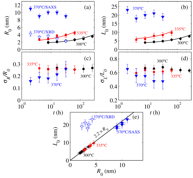
Figure 7: Parameters of the particles determined from the fit of the line scans to the short-range order model. See the text for a detailed description. The full lines in panels (a) and (b) are the graphs of fitted functions $(A+Bt)^{1/3}$ ($A$ and $B$ are suitable constants), following from the LSW theory. The straight line in (e) represents the dependence $L_{0}=2.2R_{0}$.

Finally, from the fits we determined the contrast of the refraction index $|\Delta n|$. The difference of the refraction indexes of the particle material and the matrix is proportional to the difference $\Delta\rho_{\rm el}$ in the electron densities:

$$\Delta n=-\frac{\lambda^{2}r_{\rm el}}{2\pi}\Delta\rho_{\rm el},$$

where $\lambda$ is the x-ray wavelength, $r_{\rm el}\approx 2.818$ Å^-1 is the classical electron radius, and we neglected the dispersion corrections. In Fig. 8 we plotted the contrast of the electron densities relatively to the electron density of the nominal Ti alloy (according to Tab. 1) as functions of the ageing time. In all sample series, the contrast $|\Delta\rho_{\rm el}|$ increases with ageing time. During the ageing at 300${\mkern 4.0mu{}^{\circ}\mkern-2.0mu\rm C}$ and 335${\mkern 4.0mu{}^{\circ}\mkern-2.0mu\rm C}$, the contrast values are smaller or around 10% of the nominal value, these changes can be explained by the changes in the chemical composition of the particles by several at. % of Mo, Fe, and/or Al. Of course, one single value of $|\Delta\rho_{\rm el}|$ for a given sample does not allow to determine complete chemical composition of the particles. For the highest ageing temperature of 370${\mkern 4.0mu{}^{\circ}\mkern-2.0mu\rm C}$ the contrast values following from the fit are much larger and do not correspond to any physically relevant value. This result will be discussed in Sect. 5.

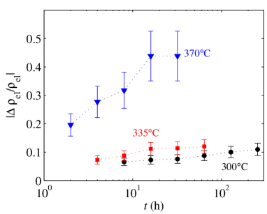
Figure 8: The difference of the electron density $\Delta\rho_{\rm el}$ of the $\omega$ particles and the $\beta$-Ti matrix relatively to the electron density of the matrix $\rho_{\rm el}$ vs ageing time.

4 Driving force of the ordering

In the previous section we demonstrated that the ordering of the particles agrees well with the short-range order model. In this section we show that the driving force of the ordering can be attributed to the minimization of the elastic interaction energy of the particles.

We have verified in our previous paper [22] that the crystal lattice around a particle is elastically deformed, the reason of the deformation is a difference between the actual lattice parameters $a_{\omega},\ c_{\omega}$ of the $\omega$ lattice of the particle and their ideal values $a_{\omega}^{(\rm id)},c_{\omega}^{(\rm id)}$ following from the topotaxy relation of the $\beta$ and $\omega$ lattices [7, 20]. Most likely, this lattice mismatch is caused by a difference in the chemical composition; during the formation and growth of $\omega$ particles the $\beta$-stabilizing impurities (Mo and Fe in our case) are expelled from the particle. Since the $\beta$-Ti matrix is highly elastically anisotropic, the local deformation field around a particle is anisotropic, too. The interaction energy of a particle pair is given by the formula [29, 30, 31]

$$E_{\rm int}=-\int_{\Omega^{\rm(B)}}{\rm d}^{3}{\bm{r}}\sigma^{\rm(A)}_{jk}({\bm{r}})\epsilon_{0jk}^{\rm(B)}({\bm{r}}),\ j,k=x,y,z.$$ (11)

The integral in this formula is calculated over the volume $\Omega^{\rm(B)}$ of particle B, $\hat{\sigma}^{\rm(A)}({\bm{r}})$ is the stress tensor in the matrix in the points belonging to $\Omega^{\rm(B)}$, caused by another particle A, and $\hat{\epsilon}_{0}^{\rm(B)}$ is the mismatch of the lattice of particle B with respect to the host lattice. Using the mismatch values

$$f_{a}=(a_{\omega}-a_{\omega}^{\mathrm{(id)}})/a_{\omega}^{\mathrm{(id)}},\ f_{c}=(c_{\omega}-c_{\omega}^{\mathrm{(id)}})/c_{\omega}^{\mathrm{(id)}}$$

defined in our previous paper and using the coordinate axes across and along the $c$-axis $[0001]_{\omega}$ of the hexagonal $\omega$ lattice, the matrix $\hat{\epsilon}_{0}^{\rm(B)}$ has the form

$$\hat{\epsilon}_{0}^{\rm(B)}=\left(\begin{array}[]{ccc}f_{a}&0&0\\ 0&f_{a}&0\\ 0&0&f_{c}\end{array}\right).$$ (12)

The stress tensor $\hat{\sigma}^{\rm(A)}({\bm{r}})$ caused by the particle A was calculated taking into account the elastic anisotropy of the host lattice and the mismatch matrix $\hat{\epsilon}_{0}^{\rm(A)}$ analogous to that in Eq. (12) using the continuum elasticity approach briefly described in the Appendix of our previous paper [22].

Assuming the typical mismatch values $f_{a}=0.002$ and $f_{c}=0.01$ found in [22] and the particle radius $R=3$nm we calculated the dependence of the interaction energy on the relative position ${\bm{r}}$ of particles (Fig. 9) in the $(1\bar{1}0)_{\beta}$ plane in the cubic $\beta$-Ti lattice. In this figure, the center of one particle is in the graph origin; since Eq. (11) is valid only for non-intersecting particles, the excluded region $|{\bm{r}}|\leq 2R$ is shaded (the grey area). The simulations were performed for all 16 combinations of the orientations of the hexagonal $c$-axes $[0001]_{\omega}$ of particles A and B with respect to the cubic $\beta$ lattice, the interaction energy plotted in this figure is averaged over all orientations.

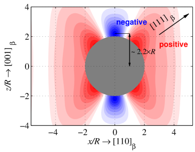
Figure 9: Dependence of the interaction energy of a particle pair on the relative position of the particles. The simulation was performed for spherical particles with the radius of 3.6nm and with the mismatch values $f_{a}=0.002,\ f_{c}=0.01$, taking into account all possible orientations of the hexagonal $[0001]_{\omega}$-axes in both particles. The grey area denotes the region, where the particles intersect. The contour step is 0.1eV.

The figure clearly indicates that minima of the interaction energy occur in six equivalent directions $\langle 100\rangle_{\beta}$ from the particle center in the distance of about $2.2\times R$. On the other hand, maxima of the interaction energy occur along eight equivalent directions $\langle 111\rangle_{\beta}$. Numerical simulations demonstrated that the anisotropy in the distribution of $E_{\rm int}$ is determined entirely by the elastic anisotropy of the host lattice and it is only very slightly affected by the anisotropy of the mismatch according to Eq. (12).

The $\langle 100\rangle_{\beta}$ directions in which the minima of $E_{\rm int}$ occur agree with the orientations of the basis vectors of the disordered array of particles determined from the SAXS data in the previous section. Therefore the anisotropy in the distribution of interaction energy indicates that the interaction energy plays a role in the self-ordering mechanism of the particles. In order to support this hypothesis we performed a simple Monte-Carlo (MC) simulation of the distribution of particles. MC simulations are widely used in the simulation of x-ray diffuse scattering and small-angle scattering. Our MC simulation program is similar to the MC simulation program for small-angle neutron scattering (SANS) [32], however, it takes into account elastic interaction between the particles.

The simulation procedure consists of the following steps:

1. we determine randomly the particle radius $R$ using a random number generator, assuming the Gamma distribution of the radii with the mean value $R_{0}$ and order $m_{R}$,

2. we choose randomly the position of the first particle in the simulation cube $D\times D\times D$,

3. we choose randomly the position of a next particle and one of four possible orientations of its hexagonal $[0001]_{\omega}$-axis,

4. we calculate the total interaction energy $E_{\rm int}$ of this particle with other particles seated in the previous steps,

5. we generate a random number $p\in[0,1]$ and we settle the particle in the position chosen in the previous step if $p<K\exp[-E_{\rm int}/(k_{B}T)]$,

6. we repeat items 3-5 $N$ times, where $N$ is the number of attempts to place a particle,

7. we repeat items 1-6 $M$ times, where $M$ is the number of simulation cubes,

8. we calculate the scattered intensity using the formula

   $$J({\bm{Q}})={\rm const.}\sum_{k=1}^{M}\left|\Omega^{\rm FT}_{R_{k}}({\bm{Q}})\sum_{n=1}^{N_{k}}{\rm e}^{-{\rm i}{\bm{Q}}.{\bm{r}}_{n}^{(k)}}\right|^{2},$$ (13)

   where ${\bm{r}}_{n}^{(k)}$ are the particle position vectors generated in items 1-5, and $N_{k}\leq N$ is the actual number of settled particle for given $k$-th simulation cube.

Therefore, the simulation procedure has the following parameters: $R_{0}$ is the mean radius of the particles, $m_{R}=(R_{0}/\sigma_{R})^{2}$ is the order of the Gamma distribution of the radii. $D$ is the size of the simulation domain and it is comparable to the coherence width and/or length of the primary x-ray beam; we took $D=50$nm. The constant $K$ was chosen so that the values $K\exp[-E_{\rm int}/(k_{B}T)]$ lie between 0 and 1, i.e. $K\approx\exp[{\rm min}(E_{\rm int})/(k_{B}T)]$ and we found that the simulation results do not depend much on $K$. The simulation temperature $T$ is not directly connected to the ageing temperature and we choose the value of $T$ to obtain the best match of the simulation results to the experimental data, namely $k_{B}T=0.5$eV. The number $N$ of the trials to set the particle positions was chosen much larger than the expected number of the particles in the $D\times D\times D$ cube; we used $N=10^{6}$. The number $M$ of the simulation cubes is determined by the ratio of the total irradiated sample volume to the coherently irradiated volume. This ratio is roughly $10^{9}$ for our experimental conditions, however we used $M=10^{3}$ to keep the calculation time in reasonable limits. The MC simulation procedure is only qualitative, since it describes properly neither the microscopic mechanism of the $\beta\rightarrow\omega$ transition, nor the growth of nucleated $\omega$ particles.

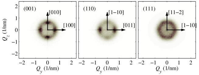
Figure 10: SAXS maps simulated in three reciprocal planes $(001),\ (110)$ and $(111)$ by the Monte-Carlo method described in text.

Figure 10 shows the examples of the simulated SAXS maps in planes $(001),\ (110)$ and $(111)$ perpendicular to the primary x-ray beam. In the simulations we took $R_{0}=3.6$ nm and $m_{R}=20$. The maps exhibit distinct side maxima, the positions of which very well coincide with the maxima in the measured maps in Fig. 2. The distance of the simulated maxima from the origin ${\bm{Q}}=0$ is inversely proportional to the mean radius $R_{0}$ of the particles; from the simulation we found that the position $Q_{\rm max}$ of the maximum at the $[100]$ axis obeys the formula

$$\frac{2\pi}{Q_{\rm max}}=L_{0}=\zeta R_{0};\zeta=2.6\pm 0.05.$$ (14)

The factor $\zeta\approx 2.6$ found from the MC simulations is slightly larger that the proportionality factor 2.2 between the position of the minimum of the interaction energy of a particle pair and the particle radius (see Fig. 9). This slight discrepancy might be caused by the fact that many particles (not only the nearest ones) contribute to the total interaction energy of a given particle. Another reason could be the asymmetry of the statistical distribution of the inter-particle distances stemming from the fact that the neighboring particles must not penetrate. However, from the SAXS data $\zeta=2.2\pm 0.1$ follows (see Fig. 7(e)).

A direct comparison of the measured and MC-simulated line scans is plotted in figure 11, where we compare the line scans extracted from the measured SAXS map of sample after 300${\mkern 4.0mu{}^{\circ}\mkern-2.0mu\rm C}$/256h ageing in figure 1 with the MC simulation performed for $R_{0}=3.6$nm and $m_{R}=20$; the simulated intensities were multiplied by a suitable constant to obtain the same heights of the side maxima. The shapes of the intensity distributions coincide well.

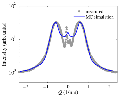
Figure 11: Comparison of the line scan extracted from the measured SAXS map in Figure 1 of sample after 300${\mkern 4.0mu{}^{\circ}\mkern-2.0mu\rm C}$/256h ageing taken in direction $[001]_{\beta}$ (points) with the result of the Monte-Carlo simulations performed for $R_{0}=3.6$nm and $m_{R}=20$ (line).

5 Discussion

The SAXS data were compared with simulations based on a phenomenological SRO model and we found a reasonably good agreement (see figure 5). From the fit we determined the mean particle radius $R_{0}$ and inter-particle distance $L_{0}$ and their dependence on the ageing time $t$. In samples aged at 300${\mkern 4.0mu{}^{\circ}\mkern-2.0mu\rm C}$ and 335${\mkern 4.0mu{}^{\circ}\mkern-2.0mu\rm C}$ the mean particle radii determined from SAXS and XRD coincide within the error limits. Furthermore, in agreement with the LSW model, the radius $R_{0}$ and the distance $L_{0}$ increase roughly as $t^{1/3}$, i.e. the total number $N$ of particles decreases as $1/t$ in these samples. The same scaling laws were also demonstrated from the XRD data in our previous paper, so that both XRD and SAXS data are consistent and they confirm the validity of the LSW model for the ageing temperatures 300${\mkern 4.0mu{}^{\circ}\mkern-2.0mu\rm C}$ and 335${\mkern 4.0mu{}^{\circ}\mkern-2.0mu\rm C}$.

The samples aged at the highest temperature of 370${\mkern 4.0mu{}^{\circ}\mkern-2.0mu\rm C}$ behave differently, namely, the mean particle distance $L_{0}$ and the mean radius $R_{0}$ determined from SAXS remained nearly constant during ageing, while the XRD-determined particle sizes are much smaller. The main reason might be that 370${\mkern 4.0mu{}^{\circ}\mkern-2.0mu\rm C}$ is temperature sufficient for $\alpha$ phase particles precipitation. It is well-known that the $\alpha$ particles have the form of platelets [20, 21] parallel to the $(0001)_{\alpha}$ basal planes perpendicular to $\langle 111\rangle_{\beta}$ directions. In SAXS, such platelets give rise to intensity streaks along $\langle 111\rangle_{\beta}$; these streaks should be visible in the SAXS intensity maps in the orientation $(110)_{\beta}$. In Fig. 12 we compare the SAXS maps of the last samples of all ageing series 300${\mkern 4.0mu{}^{\circ}\mkern-2.0mu\rm C}$, 335${\mkern 4.0mu{}^{\circ}\mkern-2.0mu\rm C}$, and 370${\mkern 4.0mu{}^{\circ}\mkern-2.0mu\rm C}$. A $[1\bar{1}1]_{\beta}$-oriented streak is clearly visible indeed only in the map of the sample aged at the highest temperature of 370${\mkern 4.0mu{}^{\circ}\mkern-2.0mu\rm C}$. Full description of these streaks and the evaluation of size of $\alpha$ platelets are beyond the scope of this paper.

In the structure model used for the fitting of the SAXS data [Fig. 5(c)] we did not include the $\alpha$ platelets, which increase the scattered intensity for small $Q$’s. Consequently, the parameters resulting from the fit of this data series are less reliable. This affects mainly the values $\Delta\rho_{\rm el}$ of the contrast of the electron density in Fig. 8. The $\Delta\rho_{\rm el}$ values of the 370${\mkern 4.0mu{}^{\circ}\mkern-2.0mu\rm C}$ series are strongly overestimated, since the scattered intensity was ascribed only to the $\omega$ particles, and a part of the intensity stems also from the $\alpha$ platelets.

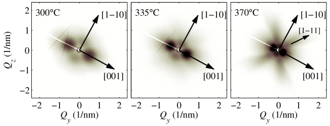
Figure 12: The SAXS intensity maps of the last samples of all three ageing series measured in the $(110)_{\beta}$ plane. The $[1\bar{1}1]_{\beta}$-oriented streak is clearly visible in the map of the sample aged at the highest temperature.

At the highest temperature (370${\mkern 4.0mu{}^{\circ}\mkern-2.0mu\rm C}$), the size of the $\omega$ particles seen by XRD is smaller than the size detected by SAXS. This temperature may be high enough for the $\omega$ particles to grow quickly at the beginning of ageing and then start to dissolve at longer ageing times (or to transform to the $\alpha$ phase). As the $\omega$ structure disappears, XRD detects smaller size of the $\omega$ particles. On the other hand, SAXS detects inhomogeneities in the electron density (i.e. chemical composition), which may remain the same even after the $\omega$ phase dissolves. However, this hypothesis would need more thorough investigation.

A gradual change in the mean chemical composition of the $\omega$ particles during ageing at 300${\mkern 4.0mu{}^{\circ}\mkern-2.0mu\rm C}$ and 335${\mkern 4.0mu{}^{\circ}\mkern-2.0mu\rm C}$ is the reason for the slight increase of the $\Delta\rho_{\rm el}$ values in Fig. 8. The increase of the chemical contrast during ageing could be ascribed to a gradual ejection of the $\beta$-stabilizing elements (Mo and Fe in our case) from the volumes of the $\omega$ particles during the ageing process. In the 370${\mkern 4.0mu{}^{\circ}\mkern-2.0mu\rm C}$ sample series, the $\Delta\rho_{\rm el}$ values are much larger and they cannot be explained by mere chemical changes. Most likely, aforementioned shell structures are the reason for these values, however this effect requires further investigation.

From the SAXS data it also follows that for ageing temperatures of 300${\mkern 4.0mu{}^{\circ}\mkern-2.0mu\rm C}$ and 335${\mkern 4.0mu{}^{\circ}\mkern-2.0mu\rm C}$ the mean particle distance $L_{0}$ is proportional to their mean radius $R_{0}$. This finding indicates that a particle-particle interaction is the reason of the ordering. Nevertheless, the phenomenological SRO model used here cannot explain fully the SAXS data. In this model the position of a given particle is affected only by the positions of neighboring particles. On the other hand, the inter-particle interaction mediated by elastic deformation of the host lattice is long-ranged and the position of a given particle is therefore affected by more distant particles as well. The SRO model fails especially between the central peak and lateral maxima, where the measured intensity exhibits a deeper dip than the simulated curve for ageing temperatures of 300${\mkern 4.0mu{}^{\circ}\mkern-2.0mu\rm C}$ and 335${\mkern 4.0mu{}^{\circ}\mkern-2.0mu\rm C}$. The shape of the intensity distribution in this region can be affected by the asymmetry of the statistical distribution of the random vectors ${\bm{L}}$ connecting neighboring particles. Another reason of the discrepancy between the measured and simulated data for small $|Q|$ could be the above-mentioned core-shell structure of the particles modifying the radial profile of the refraction index.

From the SAXS data shown above it clearly follows that the $\omega$ particles are self-ordered in a three-dimensional cubic array with the axes along $\langle 100\rangle_{\beta}$ directions. This finding differs from the conclusions in Ref. [33], where the authors claim that the particle ordering occurs along directions $\langle 111\rangle_{\beta}$. The authors support this statement by a transmission electron micrograph (TEM), where only few particles are depicted. The ordering along three $\langle 100\rangle_{\beta}$ directions may in certain cases appear as $\langle 111\rangle_{\beta}$ ordering in TEM, but the statistical relevance of SAXS data is much higher, since the number of irradiated particles in a typical SAXS experiment is several $10^{9}$, i.e. by many decades larger than in TEM. The $\langle 100\rangle_{\beta}$-oriented ordering of particles can be explained by the following simple argument. As we have shown above, the arrangement of the particles is close to a thermodynamic equilibrium, i.e. the particle positions correspond to the minima of the interaction energy of particles. As stated by Shneck et al. [31], the sign of the hydrostatic stress, i.e. the sign of the trace ${\rm Tr}(\hat{\sigma})$ of the stress tensor, is decisive for the ordering. Namely, if a particle compresses the surrounding lattice (which is the case of our samples) and ${\rm Tr}(\hat{\sigma})<0$ in the position where a new particle would appear, then the interaction energy between the existing particle and another newly formed particle is positive (repulsive). Indeed, in this case the new particle works against the stress field of the existing particle and the potential energy of the particle pair increases. Our finding is also in agreement with Ref. [17], stating that the particle ordering occurs along an elastically soft direction, i.e. along $\langle 100\rangle_{\beta}$ in our case.

We performed a series of Monte-Carlo simulations explaining qualitatively the ordering mechanism. The positions of the SAXS maxima and the linear dependence of the mean particle distance on the size of the particles following from the simulations agrees well with the SAXS data. However, a detailed comparison of the experimental data with the simulation results is not possible, since the simulation model is not fully atomistic. It does not take into account both the atomistic mechanism of the $\beta\rightarrow\omega$ transition and the kinetics of the particle formation and growth.

6 Summary

We have studied the sizes and positions of hexagonal $\omega$ Ti particles in single crystals of cubic $\beta$-Ti alloy by small-angle x-ray scattering. We determined the dependence of the particle size and distance on the ageing time and demonstrated that the particle growth can be described by the LSW model [15, 16]. We found that the particles spontaneously order creating a cubic three-dimensional array with the axes along the cubic axes $\langle 100\rangle_{\beta}$ of the host lattice. The structure of the array can be described by a phenomenological short-range order model and we demonstrated by a Monte-Carlo simulation that the driving force of the ordering is the minimization of the elastic energy of inter-particle interactions.

References

- [1] Banerjee D, Williams JC. Perspectives on titanium science and technology, Acta Materialia 2013; 61:844
- [2] Lütjering G, Williams JC. Titanium. Berlin: Springer-Verlag; 2007.
- [3] Hatt BA, Roberts JA. Acta Metall. 1960; 8: 575.
- [4] De Fontaine D. Acta Metall. 1970; 18: 275.
- [5] Williams JC, De Fontaine D, Paton NE. Met. Trans. 1973; 4: 2701.
- [6] De Fontaine D, Paton NE, Williams JC. Acta Metall. 1971; 19: 1153.
- [7] Silcock JM. Acta Metall. 1958; 6: 481.
- [8] Devaraj A, Williams REA, Nag S, Srinivasan R, Fraser HL, Banerjee R. Scripta Mater. 2009; 61: 701.
- [9] Blackburn MJ, Williams JC. Trans Metall Soc AIME. 1968; 242: 2461.
- [10] Koul MK, Breedis JF. Acta Metall. 1970; 18:579.
- [11] Ng HP, Devaraj A, Nag S, Bettles CJ, Gibson M, Fraser HL, Muddle BC, Banerjee R, Acta Mater. 2011; 59:2981.
- [12] Devaraj A, Nag S, Srinivasan R, Williams REA, Banerjee S, Banerjee R, Fraser HL. Acta Mater. 2012; 60: 596.
- [13] Cahn JW. Trans. met. Soc. AIME 1968; 242: 166.
- [14] Hilliard JE, in Phase Transformations (edited by H. I. Aaronson). p. 497. American Society for Metals, Metals Park, Ohio (1970).
- [15] Lifshitz IM, Slyozov VV. J. Phys. Chem. Solids 1961; 19: 35.
- [16] Wagner C. Zeit. Elektrochemie 1961; 65: 581.
- [17] Fratzl P, Penrose O, Lebowitz JL. J. Stat. Physics 1999; 95: 1429.
- [18] Lebowitz JL, Marro J, Kalos MH. Acta Metall. 1982; 30: 297.
- [19] Ilavsky J, Jemian PR, Allen AJ, Zhang F, Levine LE, Long GG. J. Appl. Cryst. 2009; 42:469.
- [20] Fratzl P, Langmayr F, Vogl G, Miekeley W. Acta Metall. 1991; 39: 753.
- [21] Langmayr F, Fratzl P, Vogl G, Miekeley W. Phys Rev B. 1994; 49: 11759.
- [22] Šmilauerová J, Harcuba P, Pospíšil J, Matěj Z, Holý V. Acta Mater. 2013; 61:6635.
- [23] Šmilauerová J, Pospíšil J. J. Cryst. Growth 2014; submitted.
- [24] Prima F, Vermaut P, Ansel D, Debuigne J. Mater. Trans. JIM 2000; 41: 1092.
- [25] Azimzadeh S, Rack HJ. Metall. Mater. Trans. A. 1998; 29: 2455.
- [26] Renaud G, Lazzari R, Leroy F. Surf. Sci. Reports 2009; 64: 255.
- [27] Eads JL, Millane RP. Acta Cryst. A 2001; 57: 507.
- [28] Buljan M, Radić N, Bernstorff S, Dražić G, Bogdanović-Radović I, Holý V. Acta Cryst. A 2012; 68:124.
- [29] Eshelby JD. Proc. Royal Soc. London A 1957; 241: 376.
- [30] Ardell AJ, Nicholson RB. Acta Metall. 1966; 14: 1295.
- [31] Shneck R, Alter R, Brokman A, Dariel MP. Phil. Mag. A 1992; 65: 797.
- [32] Strunz P, Gilles R, Mukherjid D, Wiedenmanne A. J. Appl. Cryst. 2003; 36: 854.
- [33] Prima F, Vermaut P, Gloriant T, Debuigne J, Ansel D. J. Mater. Sci. Letters 2002; 21: 1935.