Optimal Symbolic Controllers Determinization for BDD storage.

Abstract

Controller synthesis techniques based on symbolic abstractions appeal by producing correct-by-design controllers, under intricate behavioural constraints. Yet, being relations between abstract states and inputs, such controllers are immense in size, which makes them futile for embedded platforms. Control-synthesis tools such as PESSOA, SCOTS, and CoSyMA tackle the problem by storing controllers as binary decision diagrams (BDDs). However, due to redundantly keeping multiple inputs per-state, the resulting controllers are still too large. In this work, we first show that choosing an optimal controller determinization is an NP-complete problem. Further, we consider the previously known controller determinization technique and discuss its weaknesses. We suggest several new approaches to the problem, based on greedy algorithms, symbolic regression, and (muli-terminal) BDDs. Finally, we empirically compare the techniques and show that some of the new algorithms can produce up to $\approx 85$% smaller controllers than those obtained with the previous technique.

1 Introduction

Controller synthesis techniques based on symbolic models, such as e.g. [28, 23, 17], are becoming increasingly popular. One of the key advantages of these techniques is that they allow for synthesising correct-by-construction controllers of general nonlinear systems under intricate behavioural requirements. However, the downside of the synthesised controllers is their size as, in essence, they are huge tables mapping abstract state-space elements into input-signal values. Even for toy examples, the produced controllers can reach a size of several megabytes. In real-life applications however, they can be several orders of magnitude larger. The latter prohibits them from being used on embedded micro-controllers which typically have very limited memory resources. In general, this state-space explosion is the consequence of: (1) the number of abstract system states and inputs which are exponential in the number of dimensions and inverse-polynomial in the discretisation values; and (2) storing multiple valid input signals per abstract state.

There are numerous tools, implementing or incorporating control synthesis, such as PESSOA, SCOTS, CoSyMA, LTLMoP, TuLiP, see [18], [24], [19], [7], and [32] correspondingly. Internally, they either use an explicit control law representation in a table form or employ Reduced Ordered Binary Decision Diagrams, introduced by [4] and called RO-BDDs or simply BDDs, in an attempt to optimise the memory needed to store the synthesised control law. RO-BDDs are canonical, efficiently manipulable, and in many cases allow for compact data representation. However, their size is strongly dependent on the variables’ ordering and the problem of finding an optimal one is known to be NP-complete, as shown by [3]. To fight that issue, tools such as SCOTS and Pessoa use the state of the art RO-BDD library CUDD, see [26], which implements numerous efficient variable ordering optimisation heuristics. Yet, even when using BDDs, controllers synthesised for practical applications can easily reach hundreds of megabytes.

To our knowledge, there have been just a few attempts made to find compact but practical representations of (symbolically produced) control laws. Except for using BDDs, we are only aware of another two approaches. The first one, suggested by [27], uses piece-wise linear functions, also known as linear in segments (LIS) functions, to approximate control functions of the form $\mathnormal{g}:\mathbb{R}\rightarrow\mathbb{R}$. The approximation is considered for scalar control functions of one argument only. The main motivation for LIS is to reduce the memory footprint of implementing controllers at the cost of some on-line computations, which nonetheless are fast to perform. However, this approach does not directly scale to multiple dimensions or allows to resolve multiple-input’s non-determinism.

Another technique to reduce the control-law size, we shall refer to as LA (Local Algorithm), was proposed by [9]. It borrows ideas from algebraic decision diagrams (ADDs), see [1], for compact function representation and exploits the non-determinism inherent to safety controllers. The considered controllers are multi-valued maps $\mathnormal{g}:\mathbb{R}^{n}\rightrightarrows\mathbb{N}$. The suggested approach attempts to optimise the controller size determinizing the control law by choosing one of the possible control signals for each of the state-space points. In the selection of such unique inputs, LA maximizes the size of state-space neighbourhoods employing the same input with the expected outcome of minimizing an ADD representation of the resulting control function. However, the minimality of the ADD representation cannot be guaranteed in general by this approach, which leads us to investigate if better compression approaches may be viable.

In this paper, we first prove that the problem of choosing a size-optimal controller determinization is NP-complete. We do that assuming the BDD controller representation, but the result can be easily generalised. Next, we suggest two new determinization approaches : GA (Global Algorithm) - based on a greedy algorithm for the minimum set-cover selection problem, see [12, 5]; SR - a hybrid of ADD-based and symbolic regression techniques, powered by genetic programming, see [14, 31]. GA attempts to minimise the BDD size by maximising the number of controller states having the same input signal. It differs from LA in that, when choosing a common input for a set of states, it looks at the state-space globally, without considering the actual state positions. SR (Symbolic Regression) aims at bridging the intrinsic limitations of LA and GA by using “arbitrary” (polynomial and sigmoid in our case) functions as controller representations. This way we realise the Kolmogorov’s [16] view on data compression. Further, we combine LA and GA into a hybrid approach called LGA (Local-Global Algorithm). The idea here is that the determinization is done as in LA but, if multiple common inputs are possible, the preference is given to the one suggested by GA. In addition, we consider B-prefixed version of LGA (BLGA) which attempts for a better compression by using BDD variable reordering to produce abstract state indexes.

We perform an empirical evaluation on a number of examples from the literature. Our results show that compression-wise there is no absolute best approach. However, LGA seems, on most cases, to be providing the best compression. The SR approach, while only providing better compressions in few examples, may be most promising when looking at actual embedded deployments, if it could be pushed to remove any use of BDDs, and their overhead on actual implementations.

2 Preliminaries

2.1 Minimum set cover

The minimum set cover problem (MSC) is formulated as:

Problem 2.1 (MSC).

Given a set $X$ and a cover $\left\{S_{j}\right\}_{j\in I}$, i.e. $X\subseteq\bigcup_{j\in I}S_{j}$, where $|X|,|I|<\infty$, find the smallest subcover $I^{*}\subseteq I:X\subseteq\bigcup_{j\in I^{*}}S_{j}$.

Both, the decision and selection versions of (MSC, are known to be NP-complete. The first approximate poly-nomial-time solution for MSC was given by [12]. Later, [5] suggested an approximate poly-nomial-time solution for the generalized “minimum set weight cover problem” (MWSC); which extends MSC by that each set $S_{k}$ is assigned a weight $s_{k}\geq 0$ and the question is to find the smallest sub-cover with the minimum total weight. According to [6], the Chvátal’s algorithm time complexity is: $O\left(|I|\cdot|X|\cdot min\left(|I|,|X|\right)\right)$.

2.2 Symbolic regression

Symbolic regression is a type of regression analysis that searches for analytical expressions best fitting a given dataset of numerical data, both in terms of accuracy and simplicity. We apply this technique in order to find the smallest analytical expressions best fitting symbolic-model-based control-law functions, ensuring for the smallest control law representation. One of the most popular means for symbolic regression is genetic programming, see [13] (GP). In this work, similar to [30], we employ grammar guided genetic programming algorithms (GGGP) to find multi-dimensional analytical expressions fitting the controller’s data. In fact, the genetic process follows [29] except for that the real-value parameter tuning is done with CMA-ES [10]. To speed up the CMA-ES procedure, we use sep-CMA-ES which has a linear time and space complexity [21].

2.3 Binary Decision Diagrams

Binary Decision Diagrams (BDDs), represented with rooted directed acyclic graphs were introduced by [4], as a compact representation for boolean functions $F:\left\{0,1\right\}^{n}\rightarrow\left\{0,1\right\}$. Given $F$ with a list of arguments $\left\{v_{i}\right\}^{n}_{i=0}$, also called BDD variables or just variables, the BDD of $F$ results from the Shannon expansion thereof. The order of arguments in the signature of $F$ has clearly no impact on $F$ itself, but it has a drastic impact on the size of the resulting BDD. Finding a size-optimal BDD variable ordering was shown, in [3], to be NP-complete. Yet, there are multiple polynomial heuristics, [25], that can find a semi-optimal variable ordering. One of the most popular thereof is sifting, [22], and its variants. Given a fixed variable order, each BDD has a canonical minimum-size representation, called Reduced Ordered BDD (RO-BDD). Assuming the bottom-up BDD traversal, an RO-BDD can be obtained by the following poynomial-time algorithm, for more details see Section $4.2$ of [4]:

1. Combine terminal nodes with equal values

2. Eliminate nodes with equivalent children

3. Combine nodes with pairwise equivalent children

Multi Terminal BDDs (MTBDDs) extend BDDs in that tree’s terminal nodes allow for arbitrary labels, thus useful to encode functions of the form $F:\left\{0,1\right\}^{n}\rightarrow U$, with $|U|<\infty$. The BDD reduction algorithm is naturally extendable towards MTBDD which thus have the canonical RO-MTBDD form. For an (MT)BDD $M$, we define $R\left(.\right)$ as a reduction function producing the RO-(MT)BDD $R\left(M\right)$. Algebraic Decision Diagrams (ADDs), introduced by [1], are a synonym of MTBDDs. The current state of the art implementation for RO-(MT)BDDs is provided by the CUDD package [26].

2.4 SCOTS v2.0

SCOTS is an open source software that implements construction of symbolic models, also known as discrete abstractions, of possibly perturbed, nonlinear control systems. The tool natively supports invariance and reachability specifications as well as several control synthesis algorithms. The control laws can be stored in BDD. SCOTS comes in a form of a header-only C++ library that can be easily included in any C/C++ code but also has a MATLAB interface. We base our algorithms on the interfaces provided by the UniformGrid and SymbolicSet classes of the tool.

3 Problem statement

Consider a (possibly non-linear) discrete time control system of the form:

$$x(k+1)=f(x(k),u(k)),\;\,x(k)\in\mathcal{X}\subseteq\mathbb{R}^{n},u(k)\in\mathcal{U}\subseteq\mathbb{R}^{m}.$$

Symbolic approaches, see e.g. [28], automatically synthesize controllers in the form of discrete state transition systems. Furthermore, the resulting controllers can often be reduced to a look-up table, see [20], prescribing for each point of the state-space a set of applicable inputs guaranteeing that the control specification is satisfied. Such synthesized controllers usually take the form of the combination of a (finite) set-valued map $\mathnormal{g}:\mathcal{S}\rightrightarrows\mathcal{V}$, and quantization maps $\texttt{q}_{x}:\mathcal{X}\to\mathcal{S}$, $\texttt{q}_{u}:\mathcal{U}\to\mathcal{V}$ reducing the originally infinite state and input sets to finite sets (usually defining a grid), i.e. $\mathcal{S}\subset\mathcal{X}$, $\mathcal{S}\subset\mathcal{X}$, $|\mathcal{S}|<\infty$, $|\mathcal{V}|<\infty$. Moreover, the usual approach is to quantize each dimension of $\mathcal{X}$ and $\mathcal{U}$ independently, i.e. $\texttt{q}_{x}(x)=(\texttt{q}^{1}_{x}(x_{1}),\ldots,\texttt{q}^{n}_{x}(x_{n}))$, $\texttt{q}_{u}(u)=(\texttt{q}^{1}_{u}(u_{1}),\ldots,\texttt{q}^{n}_{u}(u_{n}))$, where each of the $\texttt{q}^{i}_{x}:\mathcal{X}_{i}\subset\mathbb{R}\to\mathcal{S}_{i}$, such that $\mathcal{S}=\mathcal{S}_{1}\times\ldots\times\mathcal{S}_{n}$, and similarly for the input quantizer. This results in controller implementations selecting at each time step $u(k)\in\mathnormal{g}\left(\texttt{q}_{x}(x(k))\right)$, see for details of such controllers [20]. Most often, the controllers synthesized do not provide a valid input for some subset $\mathcal{S}_{\emptyset}\subset\mathcal{S}$. We define the set $\mathcal{S}_{c}:=\mathcal{S}\setminus\mathcal{S}_{\emptyset}$. We may assume that there is some element $\texttt{nc}\in\mathcal{V}$ denoting a “no-input”, and thus we can define $\mathcal{S}_{\emptyset}:=\mathnormal{g}^{-1}(\texttt{nc})$.

A symbolic controller $\mathnormal{g}\subseteq\mathcal{S}\times\mathcal{V}$, by indexing the countable sets $\mathcal{S}_{i}$ and $\mathcal{V}_{i}$, can alternatively be interpreted as a relation $\mathnormal{g}\subset\mathbb{Z}_{\geq 0}\times\mathbb{Z}_{\geq 0}$. Consider $\mathcal{B}:=\left\{0,1\right\}$, and let us define a fixed-length base-$2$ bit encoding for non-negative integers $bits:\mathcal{K}\to\mathcal{B}^{b}$ for some $\mathcal{K}\subset\mathbb{Z}_{\geq 0}$, $|\mathcal{K}|<\infty$, and $b:=\left\lceil log_{2}\left(max\left(\mathcal{K}\right)\right)\right\rceil$. For $k=\left(k_{1},k_{2}\right)\in\mathnormal{g}\subset\mathbb{Z}_{\geq 0}\times\mathbb{Z}_{\geq 0}$, mapping the bit vector $\left(bits\left(k_{1}\right),bits\left(k_{2}\right)\right)$ to a boolean $1$ defines a BDD encoding of $\mathnormal{g}$. Similarly, one can construct an MTBDD encoding of $\mathnormal{g}$ by mapping $bits\left(k_{1}\right)$ to $k_{2}$.

Relating elements of $\mathcal{S}$ or $\mathcal{V}$ with $\mathbb{Z}_{\geq 0}$ can be done with an indexing function, typically defined as:

$$f_{b}\left(k_{a},\ldots,k_{b}\right):=\sum^{b}_{i=a}k_{i}\cdot\left(\prod^{i-1}_{j=a}2^{|bits\left(N_{j}\right)|}\right)\mbox{, or}$$ (1)

$$f_{s}\left(k_{a},\ldots,k_{b}\right):=\sum^{b}_{i=a}k_{i}\cdot\left(\prod^{i-1}_{j=a}N_{j}\right)$$ (2)

Here, $N_{j}$$:=$$|\mathcal{S}_{j}|$ for $j$$\in$$\overline{1,n}$, and $N_{j}$$:=$$|\mathcal{V}_{j}|$ for $j$$\in$$\overline{n\!+\!1,n\!+\!m}$; $|bits\left(N_{j}\right)|$ is the data-type size needed to enumerate intervals in $j$. Equations 2 and 1 are both used in SCOTSv2.0. The former is employed in its interface classes (UniformGrid and SymbolicSet), as it delivers smaller indexes. The latter is used for BDD encoding as it avoids bit sharing between distinct dimension interval indices.

In the present we consider the following minimisation problem aimed at finding the smallest controller determinization of a given controller $\mathnormal{g}$:

Problem 3.1 (OD).

Find the best determinization $\mathnormal{g}^{*}$ of a controller $\mathnormal{g}$ optimizing: $\mathnormal{g}^{*}=argmin_{\tilde{\mathnormal{g}}\in\mathcal{F}}\left|enc\left(\tilde{\mathnormal{g}}\right)\right|$, where

$$\mathcal{F}: = \left\{\tilde{\mathnormal{g}}:\mathbb{Z}_{\geq 0}\rightarrow\mathbb{Z}_{\geq 0}|\right.$$

$$\left.\forall s\in Dom\left(\mathnormal{g}\right):\left(\left(\tilde{\mathnormal{g}}\left(s\right)\in\mathnormal{g}\left(s\right)\right)\wedge\left(|\tilde{\mathnormal{g}}\left(s\right)|=1\right)\right)\right\},$$

$enc\left(.\right)$ encodes controllers into RO-(MT)BDDs, and $|.|$ provides the (MT)BDD size.

In theoretical derivations, as in [15], we define $|.|$ to be the number of (MT)BDD nodes. In practice, $|.|$ is the number of bits used to store the (MT)BDD by the CUDD package in the best-found, variable reordering.

4 LA on MTBDDs

[9] suggests a controller-size minimisation technique, which we call LA, that uses ideas from MTBDDs to represent the controller function in the form of a binary tree. The approach does dimension-wise binary splitting of the controller’s state-space bounding box. The areas with no-inputs are considered to allow for any input. For the areas with common inputs possible a single input is selected non-deterministically. A branch in the tree represents a state-space area with all states having common inputs (stored in terminal nodes). The determinization aims at choosing single inputs in a way minimising the depth of the tree branches. The latter is equivalent to reductions as in steps (1) and (2) of the RO-BDD construction (c.f. Section 2.3), but not (3). [9] showed that LA can lead to drastic size reductions, e.g., for “the simple thermal model of a two-room building” example the original controller required $1.000.000$ data units, whereas in the tree format it went down to $27$. Yet, in its original form this approach: (i) does not preserve the controller’s domain – neglecting basic data of safe initial states; (ii) employs a fixed state-space splitting algorithm – not using controller’s structural features; (iii) uses simple binary trees which are less efficient than MTBDDs, due to the latter compression abilities by variable reordering and their canonical reduced form. This motivates extending the approach towards MTBDDs.

LA can be adapted to quantised state-spaces, since:

1. For dimension $i$$\in$$\overline{1,n}$ and $s_{i}$$\in$$\mathcal{S}_{i}$, the bit sequence $bits\left(s_{i}\right)$, defines a binary-tree path to $s_{i}$ in $\mathcal{S}_{i}$.

2. For $s$$\in$$\mathcal{S}$, the alternating bit sequence obtained from $bits\left(s_{1}\right),\ldots,bits\left(s_{n}\right)$ defines a binary-tree path to $s$ in $\mathcal{S}$.

The latter, using bounded-length bit sequences as in Section 3, allows to encode the LA’s binary tree as an MTBDD. The size reductions obtained for the original LA are then a subset of those we get using MTBDDs, as we can: (i) obtain RO-MTBDDs, utilising all the reduction steps (ii) find a more efficient variable ordering. Let us now show that, however good, LA does not allow to utilise the full power of the MTBDD reductions due to its pure spacial orientation.

Figure 1: An example MTBDD

Consider an MTBDD encoding of some LA’s binary tree, in its original variable ordering, see Figure 1. LA traverses an MTBDD trying to find common inputs, stored in terminal nodes, for all of its sub-trees. A sub-tree with a common input can then be trivially reduced to a single terminal node. In this case however, there are no non-trivial sub-trees with common inputs, so LA has to non-deterministically choose one (arbitrary) input value per terminal node. This results in $16$ possible determinization variants, most of which would not be reducible, see e.g. Figure 2, but a few would allow for reductions; the best one is in Figure 3.

Figure 2: A non-reducible determinization

(a) After determinization

(b) After reduction

Figure 3: A reducible determinization

In this paper, we suggest alternatives and hybrid approaches to overcome this potential shortcoming of LA, see Section 6. Furthermore, to preserve information on safe initial states, we shall consider a modification of LA which forbids assignment of “any input” to “no-input” grid cells.

5 NP-completeness of determinization

Theorem 5.1.

The OD problem is NP-complete (NP-C).

Proof.

To show that OD is NP-complete we prove that:

(i) OD is NP: Consider a non-deterministic algorithm, Algorithm 1, solving the selection OD. To prove that OD is NP, one must show that Algorithm 1 has polynomial time complexity and contains a polynomial number of random guesses, each independent on the problem size. Clearly, all of the Algorithm 1 steps have polynomial time complexity. First of all, iterating over $Q\in 0,\ldots,|M|$, checking for $|M^{\prime\prime}|==Q$, and reducing $R\left(M^{\prime}\right)$, see Section 2.3, are polynomial time. Further, let us show that “guessing $M^{\prime}$ from $M$” can also be done in polynomial time with a polynomial number of Bernoulli trials. First, to visit $M$’s terminal nodes requires $\mathcal{O}\left(|M|\right)$ steps. Second, for a node, having at most $|\mathcal{U}|$ inputs, to randomly choose one input requires $\mathcal{O}\left(\left\lceil log_{2}\left(|\mathcal{U}|\right)\right\rceil\right)$ Bernoulli trials. So we conclude that OD is NP.

Input: $M$ - Controller’s MTBDD

Result: Size-optimal determinization of $M$

for $Q\in 0,\ldots,|M|$ do

       Guess $M^{\prime}$ - a determinization of $M$

       $M^{\prime\prime}\leftarrow R\left(M^{\prime}\right)$;

       if $|M^{\prime\prime}|==Q$ then

             return $M^{\prime\prime}$

       end if

      

end for

Algorithm 1 NP algorithm for selection OD

(ii) MSC is polynomial-time/space convertible to OD: For an MSC with $X:=\left\{x_{i}\right\}^{N}_{i=1}$, $S:=\left\{S_{j}\right\}^{K}_{j=1}$, $\forall j\in\overline{1,K}:S_{j}\subseteq X$, and $N,K<\infty$, consider the next three proving steps:

a) Encode MSC as an MTBDD $M$: Take a binary tree with $N$ terminal nodes, indexed by $i\in\overline{1,N}$. For each terminal node $i$ add a low (left) $t^{l}_{i}$ and a hight (right) $t^{h}_{i}$ children, such that $val\left(t^{l}_{i}\right):=\left\{j\in\overline{1,K}|x_{i}\in S_{j}\right\}$ and $val\left(t^{h}_{i}\right):=\left\{K+i\right\}$. Here, $val\left(.\right)$ is terminals’ labelling function; the low terminals encode the MSC sets; and the high terminals prevent all but low-terminals’ reductions. The resulting binary tree $T$ is a polynomial-space encoding of MSC as: $|T|=4\times N-1$. Also, this is a polynomial-time encoding, as is realisable by Algorithm 2, of time complexity $\mathcal{O}\left(N\right)$. To convert this binary tree into an MTBDD $M$, we shall interpret its non-terminal nodes as decision nodes, and its terminal nodes $t$ as value nodes, labeled with $val\left(t\right)$. This trivial conversion can also be done in polynomial time and space.

b) Solving OD for $M$ solves MSC: For the given $M$ encoding of MSC, $R\left(M^{\prime}\right)$, in Algorithm 1, can only re-combine low terminals of $M^{\prime}$ as high-terminal and thus non-terminal node reductions are prevented by the distinct high terminal node idexes. The high and non-terminals will stay intact and Algorithm 1 will effectively minimise the number of low terminals. The set $I$ of low-terminal labels of $M^{\prime\prime}$ then yields the solution for MSC as: (a) $I$ defines a sub-cover of $S$; (b) $|I|$ is minimal. The former is clear as each $x_{i}$ of $X$ is related to a low-terminal. The latter can be proved by contradiction. First, fix low-terminal node values of $M$ to those of $I$ to get an MTBDD $M_{I}$ for which $|R\left(M_{I}\right)|=3\times N-1+|I|$. Let us assume that $I$ is not a solution of MSC then there exists a sub-cover $I^{\prime}$, such that $|I^{\prime}|<|I|$. Similarly, for $M_{I^{\prime}}$ we have $|R\left(M_{I^{\prime}}\right)|=3\times N-1+|I^{\prime}|$, and thus $R\left(M_{I^{\prime}}\right)<R\left(M_{I}\right)$. The latter contradicts the fact that Algorithm 1 solves OD.

c) Decoding MSC solution from OD solution: Decoding of the MSC solution from $M^{\prime\prime}$ is straightforward: one needs to go through all of the low-terminal nodes and collect their labels. This requires linear time and space algorithm.

Finally, since MSC is NP-C, (i)&(ii), imply that OD is NP-C.

Input: $X=\left\{x_{i}\right\}^{N}$ - Set elements

Input: $S=\left\{S_{j}\right\}^{K}_{j=1}$ - Set cover

Result: The MTBDD encoding for MSC

$\mathrm{Node}\;root\leftarrow\mathrm{null}$

if $N>0$ then

       $\mathrm{Queue\langle Node\rangle}\;terms\left(N\right)\leftarrow\mathrm{empty}$

       $\mathrm{uint}\;cnt\leftarrow\mathrm{1}$

       $root\leftarrow\mathbf{new}\;\mathrm{Node\left(\right)}$

       $terms.push\_back\left(root\right)$

       while $cnt\;\not=N$ do

             $\mathrm{Node}\;term\leftarrow terms.pop\_front\left(\right)$

             $terms.push\_back\left(term.low\leftarrow\mathbf{new}\;\mathrm{Node\left(\right)}\right)$

             $terms.push\_back\left(term.high\leftarrow\mathbf{new}\;\mathrm{Node\left(\right)}\right)$

             $tcnt\leftarrow cnt+1$

       end while

      $\mathrm{uint}\;idx\leftarrow\mathrm{1}$

       while $terms\not=\mathrm{empty}$ do

             $\mathrm{Node}\;term\leftarrow terms.pop\_front\left(\right)$

             $term.low\leftarrow\mathbf{new}\;\mathrm{Node\left(\right.}get\_set\_ids(x_{idx},S\mathrm{\left.)\right)}$

             $term.high\leftarrow\mathbf{new}\;\mathrm{Node\left(\right.}\left\{K+idx\right\}\mathrm{\left.\right)}$

             $idx\leftarrow idx+1$

       end while

      

end if

return $root$;

Algorithm 2 Encode MSC as OD

∎

6 Determinization algorithms

The newly suggested determinization algorithms have various underlying ideas: GA tries to maximise the number of states with the same input, and minimise the number of different inputs as a whole, both in an attempt to maximise the chances for (MT)BDD reductions; LGA combines complementary ideas of LA and GA to reduce the number of non-deterministic choices to be taken in the former one; SR attempts to find an analytical expression fitting the controller points on the largest part of its domain to reduce the number of distinct control mode areas to be stored;

6.1 Global Approach

The GA approach is summarised in Algorithm 3, where:

1. $inputs\_to\_states\left(.\right)$ creates $C$ – the set of domain state indexes, $I$ – the set of input indexes, and $\left\{C_{j}\right\}_{j\in I}$ – the sets of states for the given inputs;

2. $get\_min\_set\_cover(.)$ implements the MSC solution algorithm for unit set weights, see Section 2.1;

3. $determinize\left(.\right)$ iterates over $I^{*}$ and for each state with the input removes all other inputs.

Input: $M$ - the controller’s MTBDD

Result: The determinized MTBDD

$\left(C,I,\left\{C_{j}\right\}_{j\in I}\right)\leftarrow inputs\_to\_states(M)$

$\mathrm{Vector}\;I^{*}\leftarrow get\_min\_set\_cover\left(C,I,\left\{C_{j}\right\}_{j\in I}\right)$

$M^{\prime}\leftarrow determinize\left(M,I^{*}\right)$

return $R\left(M^{\prime}\right)$;

Algorithm 3 The GA approach

GA differs from LA by looking at the state-space globally regardless of its’ elements location. It maximizes the number of terminal nodes with identical labels, generally leading to a reduction in the number of used labels, which should facilitate MTBDD reductions.

6.2 Local-Global Approach

Recall the MTBDD-based LA algorithm discussed in Section 4. We showed that such determinization procedure can suffer from sub-optimal non-deterministic resolutions when multiple input choices are available in some regions. LGA combines LA with GA in an attempt to improve the resulting reductions by minimising this uncertainty. In essence, the LGA approach proceeds as LA up to the moment a non-trivial set of inputs, common for a grid area, is found; then the input is chosen according to the priority-descending order of inputs, as pre-computed by the $get\_min\_set\_cover\left(.\right)$ function, see Algorithm 3.

6.3 BDD-index based Local-Global Approach

RO-(MT)BDDs achieve significant size reductions only if a “good” variable ordering is found, see Section 2.3. Given the (MT)BDD encoding, see Equation 1 of Section 3, the variable reordering swaps grid-cell index bits realising a limited form of cell re-indexing. Figure 4 shows the effects thereof on the $\mathnormal{g}\subset\mathbb{Z}_{\geq 0}\times\mathbb{Z}_{\geq 0}$ function for an LGA-determinized BDD controller of the DC motor case study, see Section 7.1. The horizontal and vertical axes of the plots correspond to the state- and input-space element indexes respectively. The distinct vertical lines on Figures 4(a) and 4(b) are the $1.000$ point marks. According to Section 3, the BDD’s range of $\mathcal{S}$ indexes is wider than that of SCOTSv2.0. Comparing $\mathnormal{g}\left(.\right)$ in RO-BDD and SCOTSv2.0 indexes, the former exhibits better data clustering. To use this to our benefit, we suggest a version of LGA, called BLGA, using the RO-BDD indexes.

(a) SCOTSv2.0 grid-cell index encoding

(b) RO-BDD grid-cell index encoding

Figure 4: DC motor: controller function

6.4 Symbolic Regression

For the SR algorithm, a set of candidate controllers is evolved using a combination of GGGP and sep-CMA-ES, c.f. references in Section 2.2, using $i_{\max}$ individuals (i.e. candidate solutions) for $N$ generations. GGGP is used to evolve the functional structure of the controller based on a grammar and sep-CMA-ES to optimize the parameters. Given a candidate controller $\mathnormal{g}_{\texttt{SR}}:\mathbb{R}^{n}\rightarrow\mathbb{R}^{m}$, the fitness function $F$ with respect to a finite set $S$ is defined as:

$$F(\mathnormal{g}_{\texttt{SR}},\mathcal{S}_{c})= \frac{\left|\left\{s\in\mathcal{S}_{c}\mid\texttt{q}_{u}(\mathnormal{g}_{\texttt{SR}}(s))\in g(s)\right\}\right|}{|\mathcal{S}_{c}|}.$$

In order to reduce the computation time, the set of states $\mathcal{S}_{c}$ is down-sampled to a set with a maximum of $\lambda$ elements. The reproduction involves selecting individuals based on tournament selection and the genetic operators crossover and mutation, in which parts of the individuals are exchanged or randomly altered respectively. More in depth descriptions of the used GGGP and sep-CMA-ES algorithms can be found in [29] and [21] respectively. After a maximum amount of generations the individual with the highest fitness is selected. For the resulting controller, it is verified for which states $s\in\mathcal{S}_{c}$ it holds that $\texttt{q}_{u}(\mathnormal{g}_{\texttt{SR}}(s))\in g(s)$. For the remaining states the inputs are determinized using GA, LA or LGA. Finally, all states and corresponding new input indexes are again stored in a BDD.

For our experiments we used the parameters in Table 1. Table 2 shows the grammar employed to determine in which space analytical expressions to fit the controllers were selected. Here $\mathrm{sgn}$ denotes the signum function and Random Real $\in\left[-1,1\right]$ creates a random real within the specified interval. The used starting symbol is $\left<\mathrm{strt}\right>$.

Table 1: SR parameters

parameters	value	explanation
$\lambda$	1000	Cardinality of down-sampled $\mathcal{S}_{c}$
$N$	50	Max. number of GGGP generations.
$M$	32	Maximum number of individuals.
$d$	7	Maximum tree depth of genotypes.
$(c_{c},c_{m})$	$(0.5,0.5)$	Crossover and mutation chance.
$\sigma_{0}$	1	Initial standard deviation.
$N_{\mathrm{ES}}$	10	Max. number of CMA-ES generations.

Table 2: Production rules $\mathcal{P}$

Nonterminal	Rules
$\left<\mathrm{strt}\right>::=$	$\left<\mathrm{const}\right>+\left<\mathrm{expr}\right>\mid\left<\mathrm{const}\right>\cdot\left<\mathrm{expr}\right>$
	$\mid\left<\mathrm{const}\right>+\left<\mathrm{const}\right>\cdot\left<\mathrm{expr}\right>$
$\left<\mathrm{expr}\right>::=$	$\left<\mathrm{lin}\right>\mid\left<\mathrm{pol}\right>\mid 0.5\mathrm{sgn}(\left<\mathrm{lin}\right>)+0.5+\left<\mathrm{expr}\right>$
	$\mid 0.5\mathrm{sgn}(\left<\mathrm{pol}\right>)+0.5+\left<\mathrm{expr}\right>$
$\left<\mathrm{lin}\right>::=$	$\left<\mathrm{const}\right>\cdot x_{1}+\dots\left<\mathrm{const}\right>\cdot x_{n}$
$\left<\mathrm{pol}\right>::=$	$\left<\mathrm{pol}\right>+\left<\mathrm{pol}\right>~{}|~{}\left<\mathrm{const}\right>\times\left<\mathrm{mon}\right>$
$\left<\mathrm{mon}\right>::=$	$\left<\mathrm{var}\right>~{}|~{}\left<\mathrm{var}\right>\times\left<\mathrm{mon}\right>$
$\left<\mathrm{var}\right>::=$	$x_{1}~{}|~{}\dots\mid x_{n}$
$\left<\mathrm{const}\right>::=$	Random Real $\in\left[-1,1\right]$

7 Empirical evaluation

7.1 Case studies

All of the considered case-studies, but the last one, are taken from the standard distribution of SCOTSv2.0: Aircraft - a DC9-30 aircraft landing maneuver, see [20]; Vehicle - a path planning problem for an autonomous vehicle, see [33] and [20]; DCDC - a boost DC-DC converter with a reach-and-stay voltage specification, see [8]; DCDC rec 1/2 - the same as DCDC but enforces a recurrence specification for two targets; DCM - a DC motor with a reach-and-stay velocity specification, see [18].The symbolic BDD controller sizes were varied by modifying the models’ input-/state-space discretisation parameters.

7.2 Software details

For the evaluation, we have realised the following software:

• A C++11 based LibLink library for Mathematica $11$, see [11], allowing to load and store BDD-based symbolic controllers of SCOTSv2.0.

• A C++11 based application implementing LA, GA, LGA, and BLGA. Our code is single-threaded as constrained by CUDD.

• A Mathematica $11$ package implementing the SR approach. This realisation is natively multi-threaded and allows for a best utilisation of the CPU cores.

7.3 Experimental setup

We have measured: (i) determinization run-time in seconds as reported by the tools; (ii) size of the determinized controllers in bytes, when stored to the file system. SR is probabilistic and therefore each of its experiments was repeated $5$ times. All other approaches are deterministic and thus their experiments were repeated only once. Overall, we have considered the algorithms on various size models, varying the discretization parameters, and thus changing:

1. The number of model inputs:

   1. GA, LA, LGA, BLGA

   2. SR on LGA determinized controllers

2. The number of model states:

   1. GA, LA, LGA, BLGA

SR was only done on LGA determinized controllers because it: (i) did not scale well with the growing number of inputs; (ii) if feasible, shall be capable of reducing deterministic controllers. The experiments were done on two machines: (A) MacBook Pro with: Intel i5 CPU (4 cores) $2.9$ GHz; $8$ GB $2133$ Mhz RAM; MacOS v$10.12.6$; (B) PC with: Intel Xeon CPU ($8$ cores) E$5-1660$ v$3$ $3.00$GHz; $32$ GB $2133$ MHz RAM; Ubuntu 16.04.3 LTS. The type $(1.a)$ experiments ran on machine (A); $(1.b)$ and $(2)$ on $(B)$.

Given, a significant difference in software realization (Mathematica v.s. C++11, multi v.s. single threaded), running SR on faster multicore machine, and that controllers’ determinization is an offline job, our run-time data: (i) is only dedicated to show the approaches’ feasibility; (ii) can only hint the actual performance differences between SR and others. This is why also the run-time for LA, GA, LGA, and BLGA is not averaged over multiple re-runs.

7.4 Results

Table 3 presents the core experimental data for models obtained by varying the number of inputs. Here, column: “SCOTS” lists information for the original controllers; “Time” is the algorithm’s run-time in seconds; “A-SR” and “M-SR”stand for the average and maximum SR values over $5$ repetitions; and “Fit %” is the fitness percentage of the SR controller’s symbolic part. To compare the compressing power of the approaches, for an algorithm $\omega$ and a case study $\nu$ we define size compression as: $C^{\nu}_{\omega}$$:=$$\left(1-|B^{\nu}_{\omega}|/|B^{\nu}|\right)*100$, where $B^{\nu}$ and $B^{\nu}_{\omega}$ stand for the original and $\omega$-determinized BDD sizes. Comparing algorithms “$\omega_{1}$ v.s. $\omega_{2}$” is done by computing a difference $\Delta^{\nu}_{\omega_{1},\omega_{2}}$$:=$$C^{\nu}_{\omega_{1}}-C^{\nu}_{\omega_{2}}$. Clearly, $\Delta^{\nu}_{\omega_{1},\omega_{2}}>0$ means $\omega_{1}$ being better than $\omega_{2}$ on $\nu$. Taking into account the A-SR experiment repetitions, we define: $C^{\nu}_{\mbox{\tiny{A-SR}}}:=E\left[C^{\nu}_{\mbox{\tiny{SR}}}\right]$.

Figure 5 contains two compression comparison sets: (i) GA, LGA, BLGA v.s. LA; and (ii) A-SR, M-SR v.s. LGA. The plot features mean compressions and the standard deviation thereof. We conclude the next compression ranking of the algorithms: 1. LGA, 2. BLGA, 3. LA, 4. GA, 5. M-SR 6. A-SR.

Figure 6 summarises the execution times for the set-up of Table 3. Relative to LA, on average: GA is $\approx 0.8$ times faster; LGA is comparable; BLGA is $\approx 1.1$ times slower; A-SR is $\approx 180$ times slower but has a huge deviation of $\approx 174$. The latter is due to probabilistic nature of SR. Note that, A-SR is multi-threaded and was run on a faster machine than the single-threaded LA. So the actual performance difference between the algorithms is more significant.

Additionally, we compared GA, LGA, BLGA and LA on up to $52$ Mb size BDD controllers, obtained by varying the number of system states. These experiments only strengthened the algorithms’ ranking conclusions implied by Figure 5. We omit further detail on that, to save space.

To conclude, we present Figure 7 summarising the compression of LGA relative to LA on all of the $67$ considered BDD controllers. Per case-study $\nu$ the compression is computed as: $C^{\nu}_{\mbox{\tiny{LGA}, {LA}}}$$:=$$\left(1-|B^{\nu}_{\mbox{\tiny{LGA}}}|/|B^{\nu}_{\mbox{\tiny{LA}}}|\right)*100$. The plot on the left of Figure 7 shows the discretized distribution of $C^{\nu}_{\mbox{\tiny{LGA}, {LA}}}$, the plot on the right shows its mean and standard deviation. Notice that, on average, LGA produces $\approx 14$% smaller controllers than LA, in the best case LGA was capable of delivering up to $\approx 85$% smaller controllers.

Table 3: Core experimental data

$$\begin{array}[]{|c|c|c|c|c|c|c|c|}\hline\cr&\lx@intercol\hfil\mbox{\tiny SCOTS}\hfil\lx@intercol\vrule\lx@intercol&\lx@intercol\hfil\mbox{\tiny LA}\hfil\lx@intercol\vrule\lx@intercol&\mbox{\tiny LGA}&\mbox{\tiny A-SR}&\mbox{\tiny M-SR}\\ \hline\cr&\mbox{\tiny\#inputs}&\mbox{\tiny\#Bytes}&\mbox{\tiny\#Bytes}&\mbox{\tiny Time}&\mbox{\tiny\#Bytes}&\mbox{\tiny Time}&\mbox{\tiny Fit \%}\\ \hline\cr\rule{0.0pt}{7.0pt}\hbox{\multirowsetup\rotatebox[origin={c}]{90.0}{\mbox{Aircraft}}}&20&2878481&150459&121.81&150316&1065,50&48.56\\ \cline{2-8}\cr\rule{0.0pt}{7.0pt}&57&9563407&193590&159.61&193055&1547,92&43.55\\ \cline{2-8}\cr\rule{0.0pt}{7.0pt}&112&8533274&236753&183.62&235273&1949,12&40.58\\ \hline\cr\hbox{\multirowsetup\rotatebox[origin={c}]{90.0}{\mbox{Vehicle}}}&49&21972&10462&1.38&9821&572,77&32.31\\ \cline{2-8}\cr&169&28537&11956&1.79&11047&614,85&27.15\\ \cline{2-8}\cr&441&54692&19430&2.86&17357&770,81&13.96\\ \cline{2-8}\cr&729&52447&18435&3.41&15793&954,53&18.14\\ \cline{2-8}\cr&1087&60757&18939&4.04&16338&1455,87&24.82\\ \hline\cr\hbox{\multirowsetup\rotatebox[origin={c}]{90.0}{\mbox{DCM}}}&2001&4951&830&2.04&371&458,61&33.14\\ \cline{2-8}\cr&10001&11957&1000&13.3&420&639,11&33.14\\ \cline{2-8}\cr&20001&24206&1166&34.65&410&742,10&24.43\\ \cline{2-8}\cr&30001&19161&1306&63.45&441&951,10&33.14\\ \cline{2-8}\cr&40001&13772&1308&94.00&449&975,50&19.82\\ \cline{2-8}\cr&50001&12921&1252&143.13&448&1121,98&33.14\\ \hline\cr\hbox{\multirowsetup\rotatebox[origin={c}]{90.0}{\mbox{DCDC}}}&2&4532&786&0.75&786&431,15&94.19\\ \cline{2-8}\cr&45&5218&1025&1.57&1025&440,99&94.19\\ \cline{2-8}\cr&89&5350&1030&2.38&1030&351,11&94.18\\ \cline{2-8}\cr&134&5272&1036&3.31&1035&450,36&94.17\\ \cline{2-8}\cr&178&5266&1036&4.11&1035&368,17&94.15\\ \cline{2-8}\cr&223&5300&1037&5.09&1036&426,01&93.55\\ \hline\cr\hbox{\multirowsetup\rotatebox[origin={c}]{90.0}{\mbox{DCDC r1}}}&2&4247&773&0.78&773&448,00&97.35\\ \cline{2-8}\cr&45&6009&915&1.48&915&417,70&97.35\\ \cline{2-8}\cr&89&5615&921&2.15&921&422,11&97.35\\ \cline{2-8}\cr&134&5768&936&2.96&930&359,65&97.35\\ \cline{2-8}\cr&178&5781&936&3.64&930&409,91&97.35\\ \cline{2-8}\cr&223&5714&936&4.48&930&428,49&95.13\\ \hline\cr\hbox{\multirowsetup\rotatebox[origin={c}]{90.0}{\mbox{DCDC r2}}}&2&2243&791&0.73&828&439,04&95.08\\ \cline{2-8}\cr&45&3685&934&2.15&937&428,78&94.51\\ \cline{2-8}\cr&89&3638&939&3.66&943&395,83&95.12\\ \cline{2-8}\cr&134&3565&949&4.98&949&361,49&94.99\\ \cline{2-8}\cr&178&3531&949&6.43&949&456,36&94.82\\ \cline{2-8}\cr&223&3549&950&8.13&950&408.70&92.91\\ \hline\cr\end{array}$$

Figure 5: Plotting $\Delta^{\nu}_{\mbox{\tiny{GA}},\mbox{\tiny{LA}}}$, $\Delta^{\nu}_{\mbox{\tiny{LGA}},\mbox{\tiny{LA}}}$, $\Delta^{\nu}_{\mbox{\tiny{BLGA}},\mbox{\tiny{LA}}}$, $\Delta^{\nu}_{\mbox{\tiny{A-SR}},\mbox{\tiny{LGA}}}$, $\Delta^{\nu}_{\mbox{\tiny{M-SR}},\mbox{\tiny{LGA}}}$

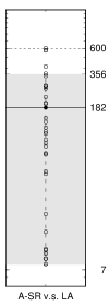
Figure 6: Execution times ratio relative to LA

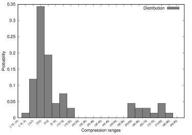
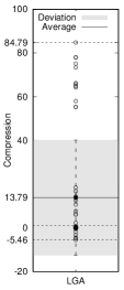
Figure 7: $C^{\nu}_{\mbox{\tiny{LGA}, {LA}}}$ distribution, deviation and average

8 Conclusions

In this work, we have considered the problem of size-optimal BDD controllers determinisation (OD), which we show to be NP-complete. Up until now, the only heuristic approach to solve OD was proposed by [9] and was based on representing the controller function as a binary tree. We have shown how that such an approach, which we call LA, can be extended to use the more size-efficient RO-(MT)BDDs data structure. In addition, we have identified examples where LA is sub-optimal due to only considering controller’s local properties. A global approach (GA), based on the minimum set cover problem solution algorithm, was proposed to remedy this. Further, a hybrid of GA and LA, called LGA, was suggested to incorporate the strengths of both approaches. To exploit the clustering of internal BDD indexes, we have come up with a BDD-index based version of LGA, called BLGA. Finally, we made an attempt of substituting the BDD-based control-law representations by functions generated using the symbolic regression (genetic-algorithm powered) approach, we refer to as SR.

All of the devised approaches were compared in compressing power and run-time by means of an extended empirical evaluation. The compression ranking of the algorithms turns out to be: 1. LGA, 2. BLGA, 3. LA, 4. GA, 5. SR. The run times of LA, GA, LGA, and BLGA are of the same order but SR is at least one to two orders of magnitude slower.

In principle, SR could allow us to eliminate BDDs completely, leading to potentially smaller functional expressions and prevent using BDD-data accessing code that, as for CUDD, is difficult (and size expensive) to port to embedded hardware. We did not manage to achieve that due to: (i) our SR realization not being powerful enough, see low fitness values in Table 3; (ii) using BDDs for storing the controller’s support, due to a decision to preserve controller’s domain. For now, we shall note that SR still looks promising for getting small and practical controllers. However, symbolic controllers seem to have structure that is not easy for SR to achieve a $100$% fitness on. So more research is needed to be done in this direction.

References

- [1] R. Iris Bahar, Erica A. Frohm, Charles M. Gaona, Gary D. Hachtel, Enrico Macii, Abelardo Pardo, and Fabio Somenzi. Algebraic decision diagrams and their applications. In Proceedings of the 1993 IEEE/ACM International Conference on Computer-aided Design, ICCAD ’93, pages 188–191, Los Alamitos, CA, USA, 1993. IEEE Computer Society Press.
- [2] S. K. Basu. Non-deterministic Algorithms, page 133. PHI Learning Private Limited, New Delhi, India, 2008.
- [3] Beate Bollig and Ingo Wegener. Improving the variable ordering of obdds is np-complete. IEEE Trans. Comput., 45(9):993–1002, September 1996.
- [4] Randal E. Bryant. Graph-based algorithms for boolean function manipulation. IEEE Trans. Comput., 35(8):677–691, August 1986.
- [5] V. Chvatal. A greedy heuristic for the set-covering problem. Mathematics of Operations Research, 4(3):233–235, 1979.
- [6] Thomas H. Cormen, Clifford Stein, Ronald L. Rivest, and Charles E. Leiserson. Introduction to Algorithms. McGraw-Hill Higher Education, 2nd edition, 2001.
- [7] Cameron Finucane, Gangyuan Jing, and Hadas Kress-Gazit. Ltlmop: Experimenting with language, temporal logic and robot control. In IEEE/RSJ Int’l. Conf. on Intelligent Robots and Systems, pages 1988 – 1993, Taipei, Taiwan, October 2010.
- [8] Antoine Girard. Controller synthesis for safety and reachability via approximate bisimulation. Automatica, 48(5):947 – 953, 2012.
- [9] Antoine Girard. Low-complexity switching controllers for safety using symbolic models*. IFAC Proceedings Volumes, 45(9):82 – 87, 2012.
- [10] Nikolaus Hansen and Andreas Ostermeier. Completely derandomized self-adaptation in evolution strategies. Evol. Comput., 9(2):159–195, June 2001.
- [11] Wolfram Research, Inc. Mathematica, Version 11.1, 2017. Champaign, IL.
- [12] Richard M. Karp. Reducibility among combinatorial problems. In Raymond E. Miller and James W. Thatcher, editors, Proceedings of a symposium on the Complexity of Computer Computations, held March 20-22, 1972, at the IBM Thomas J. Watson Research Center, Yorktown Heights, New York., The IBM Research Symposia Series, pages 85–103. Plenum Press, New York, 1972.
- [13] John R. Koza. Genetic Programming: On the Programming of Computers by Means of Natural Selection. MIT Press, Cambridge, MA, USA, 1992.
- [14] John R. Koza. Genetic programming as a means for programming computers by natural selection. Statistics and Computing, 4(2):87–112, 1994.
- [15] Marta Kwiatkowska, Gethin Norman, and David Parker. Symmetry Reduction for Probabilistic Model Checking, pages 234–248. Springer Berlin Heidelberg, Berlin, Heidelberg, 2006.
- [16] Ming Li and Paul M.B. Vitnyi. An Introduction to Kolmogorov Complexity and Its Applications. Springer Publishing Company, Incorporated, 3 edition, 2008.
- [17] Jun Liu, Necmiye Ozay, Ufuk Topcu, and Richard M. Murray. Synthesis of reactive switching protocols from temporal logic specifications. IEEE Trans. Automat. Contr., 58(7):1771–1785, 2013.
- [18] Manuel Mazo, Anna Davitian, and Paulo Tabuada. PESSOA: A Tool for Embedded Controller Synthesis, pages 566–569. Springer Berlin Heidelberg, Berlin, Heidelberg, 2010.
- [19] Sebti Mouelhi, Antoine Girard, and Gregor Gössler. Cosyma: A tool for controller synthesis using multi-scale abstractions. In Proceedings of the 16th International Conference on Hybrid Systems: Computation and Control, HSCC ’13, pages 83–88, New York, NY, USA, 2013. ACM.
- [20] Gunther Reissig, Alexander Weber, and Matthias Rungger. Feedback Refinement Relations for the Synthesis of Symbolic Controllers. IEEE Trans. Automat. Control, 62(4):1781–1796, apr 2016.
- [21] Raymond Ros and Nikolaus Hansen. A simple modification in cma-es achieving linear time and space complexity. In Parallel Problem Solving from Nature – PPSN X: 10th International Conference, Dortmund, Germany, September 13-17, 2008. Proceedings, pages 296–305, Berlin, Heidelberg, 2008. Springer Berlin Heidelberg.
- [22] Richard Rudell. Dynamic variable ordering for ordered binary decision diagrams. In Proceedings of the 1993 IEEE/ACM International Conference on Computer-aided Design, ICCAD ’93, pages 42–47, Los Alamitos, CA, USA, 1993. IEEE Computer Society Press.
- [23] Matthias Rungger, Manuel Mazo, Jr., and Paulo Tabuada. Specification-guided controller synthesis for linear systems and safe linear-time temporal logic. In Proceedings of the 16th International Conference on Hybrid Systems: Computation and Control, HSCC ’13, pages 333–342, New York, NY, USA, 2013. ACM.
- [24] Matthias Rungger and Majid Zamani. SCOTS: A tool for the synthesis of symbolic controllers. In Proceedings of the 19th International Conference on Hybrid Systems: Computation and Control, HSCC, pages 99–104, 2016.
- [25] Christoph Scholl, Bernd Becker, and Andreas Brogle. Solving the multiple variable order problem for binary decision diagrams by use of dynamic reordering techniques. Technical report, Albert-Ludwigs-University, Freiburg, D 79110 Freiburg im Breisgau, Germany, 1999.
- [26] Fabio Somenzi. CUDD: CU Decision Diagram Package, 2015. Electronically available at: http://vlsi.colorado.edu/~fabio/CUDD/.
- [27] V. Staudt. Compact representation of mathematical functions for control applications by piecewise linear approximations. Electrical Engineering, 81(3):129–134, 1998.
- [28] Paulo Tabuada. Verification and Control of Hybrid Systems: A Symbolic Approach. Springer Publishing Company, Incorporated, 1st edition, 2009.
- [29] C.F. Verdier and M. Mazo. Formal controller synthesis via genetic programming. IFAC-PapersOnLine, 2017. (To Appear).
- [30] Peter A Whigham et al. Grammatically-based genetic programming. In The workshop on genetic programming: from theory to real-world applications, pages 33–41, 1995.
- [31] M. J. Willis, H. G. Hiden, P. Marenbach, B. McKay, and G. A. Montague. Genetic programming: an introduction and survey of applications. In International Conference On Genetic Algorithms In Engineering Systems: Innovations And Applications, pages 314–319, Sep 1997.
- [32] Tichakorn Wongpiromsarn, Ufuk Topcu, Necmiye Ozay, Huan Xu, and Richard M. Murray. Tulip: A software toolbox for receding horizon temporal logic planning. In Proceedings of the 14th International Conference on Hybrid Systems: Computation and Control, HSCC ’11, pages 313–314, New York, NY, USA, 2011. ACM.
- [33] Majid Zamani, Giordano Pola, Manuel Mazo Jr., and Paulo Tabuada. Symbolic models for nonlinear control systems without stability assumptions. IEEE Trans. Automat. Contr., 57(7):1804–1809, 2012.