Shape Optimization by means of Proper Orthogonal Decomposition and Dynamic Mode Decomposition

Abstract

Shape optimization is a challenging task in many engineering fields, since the numerical solutions of parametric system may be computationally expensive. This work presents a novel optimization procedure based on reduced order modeling, applied to a naval hull design problem. The advantage introduced by this method is that the solution for a specific parameter can be expressed as the combination of few numerical solutions computed at properly chosen parametric points. The reduced model is built using the proper orthogonal decomposition with interpolation (PODI) method. We use the free form deformation (FFD) for an automated perturbation of the shape, and the finite volume method to simulate the multiphase incompressible flow around the deformed hulls. Further computational reduction is done by the dynamic mode decomposition (DMD) technique: from few high dimensional snapshots, the system evolution is reconstructed and the final state of the simulation is faithfully approximated. Finally the global optimization algorithm iterates over the reduced space: the approximated drag and lift coefficients are projected to the hull surface, hence the resistance is evaluated for the new hulls until the convergence to the optimal shape is achieved. We will present the results obtained applying the described procedure to a typical Fincantieri cruise ship.

1 Introduction

Thanks to the improved capabilities in terms of computational infrastructures in the last decade, the classical simulation-based design (SBD) has evolved into an automatic optimization procedure, that is simulation-based design optimization (SBDO). For what concerns shape optimization, the SBDO procedure consists of three main features: a shape parametrization and deformation tool, an high fidelity solver, and an optimization algorithm. In this work we present a complete SBDO pipeline of the bulbous bow of a hull advancing in calm water. It consists in an efficient shape parametrization technique, an high fidelity solver based on the finite volume method, two different model reduction techniques in order to speed up both the single high fidelity simulation and the optimization procedure, and an optimization algorithm. For what concerns shape optimization of hulls we cite among others [5, 8].

In the framework of reduced order modelling (ROM) and efficient shape parametrization techniques, a first possible choice is related to the shape morphing method itself. Since there are no particular constraints, we focus on the so-called general purpose methods, and among them we mention Free Form Deformation (FFD) [26, 12], Radial Basis Functions (RBF) interpolation [4, 17, 15, 31] or Inverse Distance Weighting (IDW) interpolation [9, 2]. Generally speaking, these methods involve the displacement of some control points in order to induce a deformation on the domain, and we identify the parameters as the displacements of the control points.

As high fidelity solver we use a finite volume method based one. We remark that this particular choice does not represent a constraint, since the pipeline proposed is independent and the solver can be considered as a black box. We simply need the flow fields of each simulation at particular time intervals. Each simulation is accelerated by the dynamic mode decomposition (DMD) technique [23, 25, 11, 13]. Originally introduced in the fluid mechanics community, the DMD has emerged as a powerful tool for analyzing the dynamics of nonlinear systems. We use it to get an estimate of the total resistance at regime simulating actually only few seconds. Finally a reduced space constructed with the POD modes is employed by the optimization algorithm for a fast evaluation of the total resistance for new parameters. In particular we use an interpolation based approach (POD with interpolation) where the new solution is obtained by interpolating the low rank solutions into the parametric space. This non intrusive choice allows us to apply the pipeline to different shape optimization problems, changing only the high fidelity solver or the parametrization technique. In this work we present the results of the optimization of the bulbous bow of a cruise ship designed and built by Fincantieri.

2 The Wave Resistance Approximation of an Hull Advancing in Calm Water

Let $\mathbb{D}\subset\mathbb{R}^{m}$ with $m\in\mathbb{N}$, be the set of parameters, and assume that it is a box in $\mathbb{R}^{m}$. Let $\mathcal{M}(\bm{x};\bm{\mu}):\mathbb{R}^{n}\to\mathbb{R}^{n}$ be a shape morphing function, mapping the reference domain $\Omega$ to the deformed domain $\Omega(\bm{\mu})$, that is $\Omega(\bm{\mu})=\mathcal{M}(\Omega;\bm{\mu})$. In the following of this work (see Section 3) we present the actual definition of $m$ and $\mathcal{M}$ for this problem.

The result of the fluid dynamic simulations will heavily depend on the specific shape of the hull. In this work we will assess the effect of the shape deformation on the total resistance, that is the main fluid dynamic performance parameter. In particular for each point in the parameter space $\mathbb{D}$, a morphing of the original hull geometry is created thanks to the function $\mathcal{M}$. The high fidelity solver based on finite volumes (see Section 4) takes these geometries as input and performs the simulation of the flow past the hull advancing in calm water for each specific hull. To come up with a resistance estimate at regime we adopt a reduction strategy that is based on the dynamic mode decomposition presented in the Section 5. With all the snapshots collected in this part of the pipeline, we construct a reduced space through a proper orthogonal decomposition with interpolation method. This space is used to perform fast evaluations of the total resistance for new parameters by the optimization algorithm.

3 Shape Morphing Based on Free Form Deformation

Free form deformation (FFD) is a widely used deformation technique both in academia and in industry. In this section we summarize the FFD-based morphing technique. For a further insight on the original formulation see [26], and for more recent works the reader can refer to [14, 20, 27, 21, 9, 22, 32]. All the algorithms have been implemented in the open source Python package PyGeM [1], which is used to perform the shape morphing in the numerical results showed in Section 7.

Basically the idea of FFD is to embed the part of the geometry we want to morph in a lattice and to deform it using a trivariate tensor-product of Bézier or B-spline functions. Thus, by moving only the control points of such lattice, we can produce a continuous and smooth deformation. The FFD procedure can be subdivided into three steps. First, we need to map the physical domain $\Omega$ to the reference domain $\widehat{\Omega}$ through the map $\psi$. Then, we move some control points $\bm{P}$ of the lattice to achieve the desired deformation, using the map $\widehat{T}$. The displacement of such points are the weights of the FFD and they represent the parameters $\bm{\mu}$. Finally we apply the back mapping from the deformed reference domain to the deformed physical domain $\Omega(\bm{\mu})$ by the map $\psi^{-1}$. So we can express the FFD map $T$ by the composition of these three maps, that is $T(\cdot,\bm{\mu})=(\psi^{-1}\circ\widehat{T}\circ\psi)(\cdot,\bm{\mu})$.

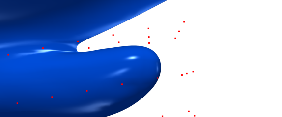
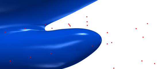
Figure 1: Bulbous bow and FFD points, before (left) and after (right) a deformation.

In Figure 1 it is possible to see the original bulbous bow on the left and an example of a deformed one on the right, respectively with the original FFD control points and with the stretched ones.

4 High Fidelity Solver Based on Finite Volume Method

Dealing with turbulent flows, the physical system is described through the Reynolds-averaged Navier Stokes (RANS) equations. In order to approximate the turbulent fluid, these equations decompose the instantaneous velocity into fluctuating and time-averaged parts [18]. We denote respectively these quantities as $u^{\prime}(x,t)$ and $\bar{u}(x,t)$, such that $u(x,t)=u^{\prime}(x,t)+\bar{u}(x,t)$. Let us put this decomposition to the incompressible continuity equation and to the momentum equation to obtain the RANS equations:

$$\begin{dcases}\frac{\partial{\bar{u}_{i}}}{\partial{x_{i}}}=0\\[-8.0pt] \frac{\partial{\bar{u}_{i}}}{\partial{t}}+\bar{u}_{j}\frac{\partial{\bar{u}_{i}}}{\partial{x_{j}}}=-\frac{1}{\rho}\frac{\partial{\bar{p}}}{\partial{\bar{x}_{i}}}+\nu\frac{\partial^{2}{\bar{u}_{i}}}{\partial{x_{j}}\partial{x_{j}}}-\frac{\partial{\overline{u^{\prime}_{i}u^{\prime}_{j}}}}{\partial{x_{j}}}\end{dcases}$$ (1)

The introduction of Reynold stress term $\overline{u^{\prime}_{i}u^{\prime}_{j}}$ requires an additional modelling in order to close the system solve it: in our work we use the popular $SST~{}k-\omega$ model [16].

In the present work, the governing equations are solved using the finite volume method (FVM). This technique is widely spread in the computational fluid dynamics community since it guarantees the conservation of all the quantities being based on the conservative form of the equations. Moreover, it is easily applicable on complex unstructured meshes. Basically, to provide the numerical solution of the partial differential equations, the space domain is subdivided into a finite number of non-overlapping polyhedra called finite volumes. The governing equations are so integrated on each finite volume and the integral values are approximated on the reference cells. For the numerical approximations of the turbulent flow over the hull surface, we use the C++ FVM-based library OpenFOAM [34].

5 Spatial and Temporal Reduction Using Dynamic Mode Decomposition

Dynamic mode decomposition (DMD) is inspired by and closely related to Koopman-operator analysis [19]. DMD was developed by Schmid in [23], and since then has emerged as a powerful tool for analyzing the dynamics of nonlinear systems, and for postprocessing spatio-temporal data in fluid mechanics [24, 25, 30]. DMD has gained popularity in the fluids community, primarily because it provides information about the dynamics of a flow, and it is applicable even when those dynamics are nonlinear [19]. Many variants of the DMD arose in the last years like multiresolution DMD, forward backward DMD, compressed DMD, and higher order DMD. For a complete review refer to [11, 13]. Since DMD relies only on the high-fidelity measurements, like experimental data and numerical simulations, it is an equation-free algorithm, and it does not make any assumptions about the underlying system.

Let us consider a sequential set of data vectors $\{\bm{x}_{1},\dots,\bm{x}_{m}\}$ where $\bm{x}_{k}\in\mathbb{R}^{n}$ for all $k\in[1,m]$. We assume that the vectors are sampled from a continuous evolution $\bm{x}(t)$, and equispaced in time. Hence, the $\bm{x}_{k}$ represents the state of the system. We also suppose that the dimension $n$ of a snapshot is larger than the number of snapshots $m$, that is $n>m$. The basic idea is that there exists a linear operator $\mathbf{A}$ (also called Koopman operator) that approximates the nonlinear dynamics of $\bm{x}(t)$, that is $\bm{x}_{k+1}=\mathbf{A}\bm{x}_{k}$. The DMD modes and eigenvalues are intended to approximate the eigenvectors and eigenvalues of $\mathbf{A}$. To obtain the minimum approximation error across all these snapshots, it is possible to arrange them in two matrices such that $\mathbf{X}=\begin{bmatrix}\mathbf{x}_{1}&\dotsc&\mathbf{x}_{m-1}\end{bmatrix}$ and $\mathbf{Y}=\begin{bmatrix}\mathbf{x}_{2}&\dotsc&\mathbf{x}_{m}\end{bmatrix}$, with $\mathbf{x}_{i}=\begin{bmatrix}x_{i}^{1}&\dotsc&x_{i}^{n}\end{bmatrix}^{\intercal}$. We underline that each column of $\mathbf{Y}$ contains the state vector at the next timestep of the one in the corresponding $\mathbf{X}$ column. We want to find $\mathbf{A}$ such that the relation between the matrices $\mathbf{X}$ and $\mathbf{Y}$ is $\mathbf{Y}\approx\mathbf{A}\mathbf{X}$. The best-fit $\mathbf{A}$ matrix is given by $\mathbf{A}=\mathbf{Y}\mathbf{X}^{\dagger}$, where the symbol ^† denotes the Moore-Penrose pseudo-inverse. Since $n>m$, the matrix $\mathbf{A}$ has $n^{2}$ elements and it is difficult to decompose it or to handle it. The DMD algorithm projects the data onto a low-rank subspace defined by the POD modes — the first left-singular vectors of the matrix $\mathbf{X}$ computed by the truncated SVD, that is $\mathbf{X}\approx\mathbf{U}_{r}\bm{\Sigma}_{r}\mathbf{V}^{*}_{r}$. We call $\mathbf{U}_{r}$ the unitary matrix whose columns contain the first $r$ modes. The low-dimensional operator is built as: $\mathbf{\tilde{A}}=\mathbf{U}_{r}^{*}\mathbf{A}\mathbf{U}_{r}=\mathbf{U}_{r}^{*}\mathbf{Y}\mathbf{V}_{r}\bm{\Sigma}_{r}^{-1}$. So we can avoid the explicit calculation of the high-dimensional operator $\mathbf{A}$, obtaining the matrix $\mathbf{\tilde{A}}\in\mathbb{C}^{r\times r}$. We can now reconstruct the eigenvectors and eigenvalues of the matrix $\mathbf{A}$ thanks to the eigendecomposition of $\mathbf{\tilde{A}}$ as $\mathbf{\tilde{A}}\mathbf{W}=\mathbf{W}\bm{\Lambda}$. In particular the elements in $\bm{\Lambda}$ correspond to the nonzero eigenvalues of $\mathbf{A}$, while the real eigenvectors, the so called exact modes [33], can be computed as $\bm{\Phi}=\mathbf{Y}\mathbf{V}_{r}\bm{\Sigma}_{r}^{-1}\mathbf{W}$. This algorithm has been implemented ‘in house’, as well as many of its variants, in an open source Python package called PyDMD [7].

6 Proper Orthogonal Decomposition with Interpolation

Reduced order methods (ROMs) have become a fundamental tool for the complex systems analysis. They make possible a remarkable reduction of the computational cost in the calculation of a solution of a parametric partial differential equation (PDE). In this section, we discuss the model reduction based on the proper orthogonal decomposition (POD), focusing on the non intrusive approach.

The basic idea is to represent the system as a linear combination of few main structures, the so called modes. Using the POD method, these structures are the orthogonal basis functions individuated through the modal analysis on the solutions vectors [10]. Hence, the high-fidelity solutions have to be computed, for some proper parameters, by the full-order solver, using the desired accuracy and the desired number of degrees of freedom. This first phase is the most computationally expensive, due to the calculation and the storage of several high-order solutions (offline phase). Then, in the online phase, these solutions are combined for an efficient and reliable approximation of the solution for a new generic parameter. In the POD Galerkin strategy — intrusive method — the discretized PDEs are projected on the space spanned by the POD modes and the significantly smaller system obtained is solved. For further details about this methodology and examples of its application, we cite [3, 28, 29]. Conversely, in a POD interpolation (PODI) approach — non intrusive method — the solutions are projected on the low dimensional space spanned by the POD modes. In this way, the solutions are described as linear combination of the modes: the coefficients of this combination, the so called modal coefficients, are interpolated in order to provide the coefficients for any point belonging to the parameter space. With the interpolated coefficients and the modes we can finally compute the approximated solution. PODI method has the advantage to require only the solutions vectors, with no assumption on the underlying system, though the accuracy of the approximation depends on the interpolation method chosen.

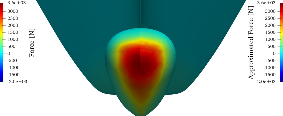
Figure 2: A comparison between the numerical solution from the full-order model (left) and the numerical solution from the reduced model using a PODI strategy. The picture represents the force on the hull domain.

Within this work, we adopted the PODI method in order to maintain the optimization pipeline completely independent from the full-order model. The method has been implemented in the open source Python package EZyRB [6]. In Figure 2 we show an example of the numerical solution computed with this software, compared with the high-fidelity validation from the full-order model.

7 Numerical Results

In this section we present the numerical results obtained by the application of the above described pipeline on a Fincantieri cruise ship. We adopted the FFD technique for the surface deformation: we used 5 different parameters and we set the parameter space dimensions to obtain physically meaningful hulls. We generated 62 different deformed shapes, 32 corresponding to the vertices of the parameter space and 30 corresponding to uniform sampling points in the parameter space. We simulated the advance in calm water of all these deformed hulls at a constant speed corresponding to Fr = 0.2 by using the FV method, collecting 20 snapshots of the full-order simulation between the 50th and 60th second. These snapshots, containing the pressure and shear stress fields on the hull surface, have been used to estimate the hull resistance at regime by the DMD algorithm. Exploiting the correlation between the parametric points and the reconstructed solutions, we created the reduced space with the PODI strategy, interpolating the modal coefficients with radial basis functions with multiquadric kernel. The low computational cost of a single parametric solution allows us to apply expensive global optimization algorithms, such as surrogate-based optimization. This algorithm generates several designs of experiment and interpolates the objective function evaluated in these points to create a surrogate model, then this model is evaluated until convergence to the optimal point. The procedure iterates until the accuracy of the surrogate model is reached. This method allows a quasi real-time optimization. Figure 3 the optimized bulb compared to the original one. After the optimization loop, the best hull has been used as input for a further high-fidelity simulation, to validate the numerical solution of the reduced model. The automatic optimization procedure reached a remarkable reduction in the hull resistance: comparing the full-order solutions, the optimized ship resistance is 2% lower compared to the original ship, while the error between the high-fidelity and the PODI solution, evaluated in the optimal parametric point, is around the 8%. Despite the error is bigger than the resistance reduction, we underline that we mainly focused on the minimization of the total resistance, hence the error was not involved in the stop criteria. We recall that the accuracy of the reduced model depends on the richness of the database of the high-fidelity solutions. Thus the PODI method can reach the wanted precision enriching the database, for example by adding iteratively the high-fidelity validation computed in the optimal point. Regarding this work, the reached reduction was enough to demonstrate a concrete application of the optimization pipeline.

Figure 3: Three sections of the bulbous bow with the original shape (red) against the optimized one (blue).

8 Conclusions and Perspectives

In this work we presented a shape optimization pipeline combining DMD and POD with interpolation. We applied it to the problem of minimizing the total resistance of a hull advancing in calm water varying the shape of the bulbous bow of a Fincantieri cruise ship. The numerical results show that with only 5 parameters we achieved a reduction of the resistance of 2%, remaining independent from the solver. Several enhancements on the pipeline could be foreseen. Among the possible ones, we mention a deeper investigation on the interpolation method and on the optimization algorithm itself.

References

- [1] PyGeM: Python Geometrical Morphing. Available at: https://github.com/mathLab/PyGeM.
- [2] F. Ballarin, A. D’Amario, S. Perotto, and G. Rozza. A pod-selective inverse distance weighting method for fast parametrized shape morphing. arXiv:1710.09243, 2017.
- [3] F. Ballarin and G. Rozza. POD–Galerkin monolithic reduced order models for parametrized fluid-structure interaction problems. International Journal for Numerical Methods in Fluids, 82(12):1010–1034, 2016.
- [4] M. D. Buhmann. Radial basis functions: theory and implementations, volume 12. CUP, 2003.
- [5] D. D’Agostino, A. Serani, E. F. Campana, and M. Diez. Nonlinear methods for design-space dimensionality reduction in shape optimization. In International Workshop on Machine Learning, Optimization, and Big Data, pages 121–132. Springer, 2017.
- [6] N. Demo, M. Tezzele, and G. Rozza. EZyRB: Easy Reduced Basis method. The Journal of Open Source Software, 3(24):661, 2018.
- [7] N. Demo, M. Tezzele, and G. Rozza. PyDMD: Python Dynamic Mode Decomposition. The Journal of Open Source Software, 3(22):530, 2018.
- [8] M. Diez, E. F. Campana, and F. Stern. Design-space dimensionality reduction in shape optimization by Karhunen–Loève expansion. Computer Methods in Applied Mechanics and Engineering, 283:1525–1544, 2015.
- [9] D. Forti and G. Rozza. Efficient geometrical parametrisation techniques of interfaces for reduced-order modelling: application to fluid–structure interaction coupling problems. International Journal of Computational Fluid Dynamics, 28(3-4):158–169, 2014.
- [10] J. S. Hesthaven, G. Rozza, B. Stamm, et al. Certified reduced basis methods for parametrized partial differential equations. Springer, 2015.
- [11] J. N. Kutz, S. L. Brunton, B. W. Brunton, and J. L. Proctor. Dynamic Mode Decomposition: Data-Driven Modeling of Complex Systems. SIAM, 2016.
- [12] T. Lassila and G. Rozza. Parametric free-form shape design with PDE models and reduced basis method. Computer Methods in Applied Mechanics and Engineering, 199(23–24):1583–1592, 2010.
- [13] S. Le Clainche and J. M. Vega. Higher order dynamic mode decomposition. SIAM Journal on Applied Dynamical Systems, 16(2):882–925, 2017.
- [14] M. Lombardi, N. Parolini, A. Quarteroni, and G. Rozza. Numerical simulation of sailing boats: Dynamics, FSI, and shape optimization. In Variational Analysis and Aerospace Engineering: Mathematical Challenges for Aerospace Design, pages 339–377. Springer, 2012.
- [15] A. Manzoni, A. Quarteroni, and G. Rozza. Model reduction techniques for fast blood flow simulation in parametrized geometries. International journal for numerical methods in biomedical engineering, 28(6-7):604–625, 2012.
- [16] F. R. Menter. Two-equation eddy-viscosity turbulence models for engineering applications. AIAA journal, 32(8):1598–1605, 1994.
- [17] A. Morris, C. Allen, and T. Rendall. CFD-based optimization of aerofoils using radial basis functions for domain element parameterization and mesh deformation. International Journal for Numerical Methods in Fluids, 58(8):827–860, 2008.
- [18] O. Reynolds. On the dynamical theory of incompressible viscous fluids and the determination of the criterion. Philosophical Transactions of the Royal Society of London. A, 186:123–164, 1895.
- [19] C. W. Rowley, I. Mezić, S. Bagheri, P. Schlatter, and D. S. Henningson. Spectral analysis of nonlinear flows. Journal of fluid mechanics, 641:115–127, 2009.
- [20] G. Rozza, A. Koshakji, and A. Quarteroni. Free Form Deformation techniques applied to 3D shape optimization problems. Communications in Applied and Industrial Mathematics, 4, 2013.
- [21] F. Salmoiraghi, F. Ballarin, L. Heltai, and G. Rozza. Isogeometric analysis-based reduced order modelling for incompressible linear viscous flows in parametrized shapes. Advanced Modeling and Simulation in Engineering Sciences, 3(1):21, 2016.
- [22] F. Salmoiraghi, A. Scardigli, H. Telib, and G. Rozza. Free form deformation, mesh morphing and reduced order methods: enablers for efficient aerodynamic shape optimization. arXiv:1803.04688, 2017.
- [23] P. J. Schmid. Dynamic mode decomposition of numerical and experimental data. Journal of fluid mechanics, 656:5–28, 2010.
- [24] P. J. Schmid. Application of the dynamic mode decomposition to experimental data. Experiments in fluids, 50(4):1123–1130, 2011.
- [25] P. J. Schmid, L. Li, M. P. Juniper, and O. Pust. Applications of the dynamic mode decomposition. Theoretical and Computational Fluid Dynamics, 25(1-4):249–259, 2011.
- [26] T. Sederberg and S. Parry. Free-Form Deformation of solid geometric models. In Proceedings of SIGGRAPH - Special Interest Group on GRAPHics and Interactive Techniques, pages 151–159, 1986.
- [27] D. Sieger, S. Menzel, and M. Botsch. On shape deformation techniques for simulation-based design optimization. In New Challenges in Grid Generation and Adaptivity for Scientific Computing, pages 281–303. Springer, 2015.
- [28] G. Stabile, S. Hijazi, A. Mola, S. Lorenzi, and G. Rozza. POD-Galerkin reduced order methods for CFD using Finite Volume Discretisation: vortex shedding around a circular cylinder. Communications in Applied and Industrial Mathematics, 8(1):210–236, 2017.
- [29] G. Stabile and G. Rozza. Finite volume POD-galerkin stabilised reduced order methods for the parametrised incompressible Navier–Stokes equations. Computers & Fluids, Feb 2018.
- [30] P. Stegeman, A. Ooi, and J. Soria. Proper orthogonal decomposition and dynamic mode decomposition of under-expanded free-jets with varying nozzle pressure ratios. In Instability and Control of Massively Separated Flows, pages 85–90. Springer, 2015.
- [31] M. Tezzele, F. Ballarin, and G. Rozza. Combined parameter and model reduction of cardiovascular problems by means of active subspaces and POD-Galerkin methods. arXiv:1711.10884, 2017.
- [32] M. Tezzele, F. Salmoiraghi, A. Mola, and G. Rozza. Dimension reduction in heterogeneous parametric spaces with application to naval engineering shape design problems. arXiv:1709.03298, 2017.
- [33] J. Tu, C. Rowley, D. Luchtenburg, S. Brunton, and N. Kutz. On dynamic mode decomposition: Theory and applications. Journal of Computational Dynamics, 1(2):391–421, 2014.
- [34] H. G. Weller, G. Tabor, H. Jasak, and C. Fureby. A tensorial approach to computational continuum mechanics using object-oriented techniques. Computers in physics, 12(6):620–631, 1998.