Dynamic magneto-optic coupling in a ferromagnetic nematic liquid crystal

Abstract

Hydrodynamics of complex fluids with multiple order parameters is governed by a set of dynamic equations with many material constants, of which only some are easily measurable. We present a unique example of a dynamic magneto-optic coupling in a ferromagnetic nematic liquid, in which long-range orientational order of liquid crystalline molecules is accompanied by long-range magnetic order of magnetic nanoplatelets. We investigate the dynamics of the magneto-optic response experimentally and theoretically and find out that it is significantly affected by the dissipative dynamic cross-coupling between the nematic and magnetic order parameters. The cross-coupling coefficient determined by fitting the experimental results with a macroscopic theory is of the same order of magnitude as the dissipative coefficient (rotational viscosity) that governs the reorientation of pure liquid crystals.

Fluids with an apolar nematic orientational ordering – nematic liquid crystals (NLCs) – are well known and understood, with properties useful for different types of applications goodby . As a contrast, possible existence of fluids with a polar orientational order, thus of a lower symmetry than NLCs, has been always intriguing. An electrically polar nematic liquid was theoretically discussed born as early as 1910s, but such a phase has never been observed. Similarly, vectorial magnetic ordering, i.e., ferromagnetism, is a phenomenon that occurs in solids and has been for the longest time considered hardly compatible with the liquid state.

Quite recently, however, ferromagnetic NLCs have been realized in suspensions of magnetic nanoplatelets in NLCs alenkanature ; shuaiNC ; smalyukhPNAS and their macroscopic static properties were characterized in detail alenkasoftmatter . These systems possess two order parameters giving rise to two preferred directions – the nematic director n (denoting the average orientation of liquid crystalline molecules) and the spontaneous magnetization $\bf M$ (describing the density of magnetic moments of the nanoplatelets) – that are coupled statically as well as dynamically. As a consequence, optical and magnetic responses are coupled in these materials, which makes them particularly interesting in the multiferroic context: optical properties can be manipulated with a weak external magnetic field (a strong magneto-optic effect) and conversely, the spontaneous magnetization can be reoriented by an external electric field (the converse magnetoelectric effect). Note that subjecting the liquid crystal to an external electric field is the usual means of controlling the nematic director in optical applications.

The search for a ferromagnetic nematic phase started when Brochard and de Gennes bropgdg suggested and discussed a ferromagnetic nematic phase combining the long range nematic orientational order with long range ferromagnetic order in a fluid system. The synthesis and experimental characterization of ferronematics and ferrocholesterics, a combination of low-molecular-weight NLCs with magnetic liquids leading to a superparamagnetic phase, started immediately and continued thereafter rault ; amer ; kopcansky ; ouskova ; buluy ; podoliak (compare also Ref. reznikov for a recent review). These studies were making use of ferrofluids or magnetorheological fluids (colloidal suspensions of magnetic particles) rosensweig ; their experimental properties rosensweig ; odenbach2004 have been studied extensively in modeling burylovII ; mario2001 ; luecke2004 ; hess2006 ; sluckin2006 ; mario2008 ; klapp2015 using predominantly macroscopic descriptions burylovII ; mario2001 ; luecke2004 ; hess2006 ; sluckin2006 ; mario2008 .

On the theoretical side the macroscopic dynamics of ferronematics was given first for a relaxed magnetization jarkova2 followed by taking into account the magnetization as a dynamic degree of freedom jarkova as well as incorporating chirality effects leading to ferrocholesterics fink2015 . In parallel a Landau description including nematic as well as ferromagnetic order has been presented hpmhd .

In this Letter we describe experimentally and theoretically the dynamic properties of ferromagnetic NLCs, focusing on the coupled evolution of the magnetization and the director fields actuated by an external magnetic field. The dynamic coupling between $\bf M$ and $\bf n$ has been a complete blank to this day. It has been known that it is allowed by symmetry and the rules of linear irreversible thermodynamics, and was cast in a definite form theoretically jarkova as a prediction. Here we demonstrate that these coupling terms influence decisively the dynamics. Quantitative agreement between the experimental results and the model is reached and a dissipative cross-coupling coefficient between the magnetization and the director is accurately evaluated. It is shown that this cross-coupling is crucial to account for the experimental results thus underscoring the importance of such cross-coupling effects in this recent soft matter system.

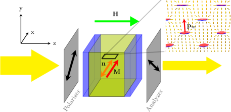
Figure 1: (Color online) Sketch of the experimental set-up and definition of coordinate axes. The thick yellow arrows indicate the direction of the light passing through the polarizer and the analyzer. In the absence of an applied magnetic field (${\bf H}$, $z$ direction), the equilibrium director (${\bf n}$) and magnetization (${\bf M}$) fields are only slightly pretilted from the $x$ direction. Inset: distortion of the NLC director (ellipsoids, schematic) prevents flocculation of the suspended nanoplatelets carrying a magnetic moment ${\bf p}_{m}$ parallel to $\bf n$ in equilibrium.

The suspension of magnetic nanoplatelets in the NLC pentylcyanobiphenyl (5CB, Nematel) was prepared as described in Ref. alenkasoftmatter . The magnetic platelets with an average diameter of 70 nm and thickness of 5 nm, made of barium hexaferrite doped with scandium, were covered by the surfactant dodecylbenzenesulphonic acid (DBSA). The surfactant induced perpendicular anchoring of 5CB molecules on the platelet surface leading to parallel orientation of the platelet magnetic moments and the nematic director, Fig. 1 (inset). The volume concentration of the platelets in 5CB, determined by measuring the saturated magnetization of the suspension, was $\sim 3\times 10^{-4}$, which corresponds to the magnetization magnitude of $M_{0}\sim 50$ A/m. The suspension was put in a liquid crystal cell with thickness $d\sim 20\,\mu$m, inducing planar homogeneous orientation of n along the rubbing direction $x$, Fig. 1. During the filling process a magnetic field (not shown) of 8 mT was applied in the direction of the rubbing, so that a magnetic monodomain sample was obtained. In the absence of an external magnetic field the spontaneous magnetization ${\bf M}$ was parallel to ${\bf n}$.

The suspension exhibits a strong magneto-optic effect. For example, when a magnetic field $\bf H$ is applied perpendicularly to ${\bf M}$ ($z$ direction), it exerts a torque on the magnetic moments, i.e., on the platelets, and causes their reorientation. Because the orientations of the platelets and the director are coupled through the anchoring of the NLC molecules on the platelet’s surface, also ${\bf n}$ reorients, which is observed as an optic response. In Fig. 2 (left) the response of $\bf M$ and $\bf n$ is shown schematically; note the small angle between ${\bf M}$ and ${\bf n}$ in equilibrium.

The reorientation of ${\bf n}$ is detected optically by measuring the phase difference $\phi$ between transmitted extraordinary and ordinary light alenkasoftmatter , Fig. 1. The normalized phase difference $r({H})=1-{\phi({H})/\phi_{0}}$, where $\phi_{0}$ is the phase difference at zero magnetic field, is shown in Fig. 2 (right) as a function of the applied magnetic field. While in ordinary nonpolar NLCs a finite threshold field needs to be exceeded to observe a response to the external field, in the ferromagnetic case the response is thresholdless.

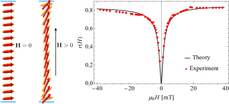
Figure 2: (Color online) Left: response of the magnetization (red arrows) and the director (ellipsoids) to the external magnetic field $\bf H$ applied in the $z$ direction. Right: equilibrium normalized phase difference $r(H)$ as a function of the magnetic field $\mu_{0}H$, fitted by the static model.

The static response was quantitatively studied in Ref. alenkasoftmatter . Here we focus on the dynamics of the response. Fig. 3 (top) shows two examples of the measured time dependence of the normalized phase difference $r(H)$.

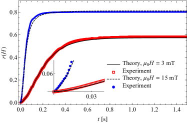
Figure 3: (Color online) Top: time evolution of the normalized phase difference, $r(H)$, fitted by the dynamic model Eqs. (2)-(11). The linear-quadratic onset of $r(H)$ is in accord with the analytic result given in Eq. (13). Bottom: the corresponding theoretical time evolution of $M_{z}/M_{0}$, initially growing linearly as expected analytically.

The time dependences of $r(H)$ acquired systematically for several field strengths were fitted by a squared sigmoidal function

$$f(t)=C^{\prime}\left[1-\frac{1+C}{1+C\exp(-2t/\tau)}\right]^{2}$$ (1)

to obtain the characteristic switching time $\tau(H)$. Remarkably, its inverse shows a linear dependence on $H$, Fig. 4. Considering only a static (energetic) coupling between ${\bf M}$ and ${\bf n}$ one would expect that $1/\tau(H)$ saturates already at low fields as the transient angle between ${\bf M}$ and ${\bf n}$ gets larger.

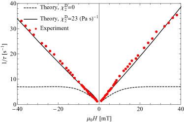
Figure 4: (Color online) The inverse of the switching time, $1/\tau(H)$, as a function of the magnetic field $\mu_{0}H$, extracted from the experimental data and the theoretical results using the fitting function Eq. (1). Without the dynamic cross-coupling, $1/\tau(H)$ saturates already at low fields (dashed).

In a minimal theoretical model we include the magnetization field ${\bf M}({\bf r})$ and the director field ${\bf n}({\bf r})$ and focus on the essential ingredients of their dynamics necessary to capture the experimental results. For a complete set of macroscopic dynamic equations for ferronematics we refer to Ref. jarkova and for ferromagnetic NLCs to Ref. tilenlong .

The statics is described by a free energy density $f({\bf M},{\bf n},\nabla{\bf n})$,

$$f=-\mu_{0}{\bf M}\cdot{\bf H}-{\textstyle\frac{1}{2}}A_{1}({\bf M}\cdot{\bf n})^{2}+{\textstyle\frac{1}{2}}A_{2}\left(|{\bf M}|-M_{0}\right)^{2}+f^{F},$$ (2)

where $\mu_{0}$ is the magnetic constant, ${\bf H}=H\hat{{\bf e}}_{z}$ is the homogeneous magnetic field fixed externally (since $H\gg M_{0}$), $A_{1,2}>0$ will be assumed constant and the Frank elastic energy of director distortions is degennesbook

$$f^{F} = {\textstyle\frac{1}{2}}K_{1}(\nabla\cdot{\bf n})^{2}+{\textstyle\frac{1}{2}}K_{2}\left[{\bf n}\cdot(\nabla\times{\bf n})\right]^{2}$$ (3)

$$+ {\textstyle\frac{1}{2}}K_{3}\left[{\bf n}\times(\nabla\times{\bf n})\right]^{2},$$

with positive elastic constants for splay ($K_{1}$), twist ($K_{2}$), and bend ($K_{3}$). To a good approximation, one can assume that $|{\bf M}|=M_{0}$. We will however allow for small variations of $|{\bf M}|$ (large $A_{2}$), which is physically sound and technically convenient.

At the cell plates, the director is anchored with a finite surface anchoring energy rapini , $f^{S}=-{\textstyle\frac{1}{2}}W({\bf n}_{S}\cdot{\bf n})^{2}$, where $W$ is the anchoring strength and ${\bf n}_{S}=\hat{{\bf e}}_{z}\sin\varphi_{s}+\hat{{\bf e}}_{x}\cos\varphi_{s}$ is the preferred direction specified by the director pretilt angle $\varphi_{s}$.

The total free energy is $F=\int\!\!f\,{\rm d}V+\int\!\!f^{S}\,{\rm d}S$ and the equilibrium condition requires $\delta F=0$.

The dynamics is governed by the balance equations pleinerbrandchapter ; jarkova

$$\dot{M}_{i}+X_{i}^{R}+X_{i}^{D} = 0,$$ (4)

$$\dot{n}_{i}+Y_{i}^{R}+Y_{i}^{D} = 0,$$ (5)

where the quasi-currents have been split into reversible ($X_{i}^{R}$, $Y_{i}^{R}$) and irreversible, dissipative ($X_{i}^{D}$, $Y_{i}^{D}$) parts. The reversible (dissipative) parts have the same (opposite) behavior under time reversal as the time derivatives of the corresponding variables, i.e., Eqs. (4)-(5) are invariant under time reversal if and only if dissipative quasi-currents are zero.

The quasi-currents are expressed as linear combinations of conjugate quantities (thermodynamic forces), which in our case are the molecular fields

$$h_{i}^{M} \equiv \frac{\delta f}{\delta M_{i}}=\frac{\partial f}{\partial M_{i}},$$ (6)

$$h_{i}^{n} \equiv \delta_{ik}^{\perp}\frac{\delta f}{\delta n_{k}}=\delta_{ik}^{\perp}\left(\frac{\partial f}{\partial n_{k}}-\partial_{j}\Phi_{kj}\right),$$ (7)

where $\Phi_{kj}={\partial f/\partial(\partial_{j}n_{k})}$ and $\delta_{ik}^{\perp}=\delta_{ik}-n_{i}n_{k}$ projects onto the plane perpendicular to the director owing to the constraint ${\bf n}^{2}=1$. These molecular fields can be viewed as exerting torques on M and n. In equilibrium they are zero, yielding the static solutions for $\bf M$ and $\bf n$, Fig. 2. When they are nonzero, they generate quasi-currents, which drive the dynamics through Eqs. (4)-(5). If there is no dynamic cross-coupling, ${\bf h}^{M}$ drives the dynamics of $\bf M$ and ${\bf h}^{n}$ drives the dynamics of n. In Fig. 4, $1/\tau(H)$ for this case is shown dashed. The clear deviation from the experiments indicates the importance of the dynamic cross-coupling.

We will focus on the dissipative quasi-currents as they have a direct relevance for the explanation of the experimental results discussed. The dissipative quasi-currents read jarkova

$$X_{i}^{D} = b_{ij}^{D}h_{j}^{M}+\chi_{ji}^{D}h_{j}^{n},$$ (8)

$$Y_{i}^{D} = \frac{1}{\gamma_{1}}h_{i}^{n}+\chi_{ij}^{D}h_{j}^{M},$$ (9)

where

$$\chi_{ij}^{D} = \chi_{1}^{D}\delta_{ik}^{\perp}M_{k}n_{j}+\chi_{2}^{D}\delta_{ij}^{\perp}M_{k}n_{k},$$ (10)

$$b_{ij}^{D} = b_{\parallel}^{D}n_{i}n_{j}+b_{\perp}^{D}\delta_{ij}^{\perp}$$ (11)

and we will everywhere disregard the biaxiality of the material tensors that takes place when ${\bf n}\nparallel{\bf M}$. We speculate that a possible origin of this dissipative dynamic coupling between ${\bf M}$ and ${\bf n}$ is a microscopic fluid flow localized in the vicinity of the rotating magnetic platelets.

The system Eqs. (4)-(5) is discretized in the $z$ direction and solved numerically. By fitting the static data to the model, Fig. 2 (right), we extract the values for the anchoring strength $W\sim 2.3\times 10^{-6}$ J/m², the pretilt angle $\varphi_{s}\sim 0.05$ and the static magnetic coupling coefficient $A_{1}\sim 130\mu_{0}$. The agreement between the static experimental data and the model underscores that we have solid ground for the analysis of the dynamics.

In Fig. 3 (top) the measured time dependence of the normalized phase difference $r(H)$ is compared alenkasoftmatter to the model for two rather distinct values of the magnetic field. The fits are performed by varying the values of the dynamic parameters subject to stability restrictions, while keeping the values of $W$, $\varphi_{s}$, and $A_{1}$ fixed as determined from the statics. The model captures the dynamics very well for all times from the onset to the saturation. The extracted values of the dynamic parameters are $\gamma_{1}\sim 0.03$ Pa s, $b_{\perp}^{D}\sim 7.8\times 10^{4}$ Am/Vs² and $\chi_{2}^{D}\sim 23$ (Pa s)^-1, which safely meets the positivity condition of the entropy production $|\chi_{2}^{D}|<\sqrt{b_{\perp}^{D}/(\gamma_{1}M_{0}^{2})}\sim 32$  (Pa s)^-1. The remaining two dynamic parameters do not affect the dynamics significantly and are set to $b^{D}_{\parallel}=b^{D}_{\perp}$ and $\chi_{1}^{D}=0$.

Fig. 3 (bottom) shows the corresponding theoretical time dependence of the normalized $z$ component of the magnetization, which is not measured due to insufficient time resolution of the vibrating sample magnetometer alenkasoftmatter (LakeShore 7400 Series VSM, several seconds are required for ambient magnetic noise averaging).

Initially, ${\bf n}$ is homogeneous and aligned with ${\bf M}$, such that ${\bf h}^{n}$ is zero and the director dynamics in Eq. (9) is due to ${\bf h}^{M}$ alone. For small times when ${\bf M}$ and ${\bf n}$ are only slightly pretilted from the $x$ direction, it thus follows from Eqs. (5) and (9) that

$$n_{z}(t)\approx\varphi_{s}+\chi_{2}^{D}M_{0}\mu_{0}H\,t$$ (12)

and hence alenkasoftmatter

$$r(H) = \frac{n_{0e}(n_{0e}+n_{0})}{2n_{0}^{2}}[(\chi_{2}^{D}M_{0}\mu_{0}H)^{2}t^{2}+2\varphi_{s}\chi_{2}^{D}M_{0}\mu_{0}Ht]$$ (13)

$$\equiv k^{2}t^{2}+pt,$$

which is also revealed by Fig. 3 (top, inset); $n_{0}$ and $n_{0e}$ are the ordinary and the extraordinary refractive indices. In principle, $k^{2}$ contains a small static coupling ($A_{1}$) correction linear in the pretilt, which is however within the error margin and is neglected. The initial dynamics of the director and the behavior of $r(H)$ are thus governed by the dissipative dynamic cross-coupling between director and magnetization, Eq. (9), described by the parameter $\chi_{2}^{D}$.

Fitting Eq. (13) to the initial time evolution of measured normalized phase differences for several values of the magnetic field $\mu_{0}H$, we determine the parameters $k$ and $p$, Fig. 5, and extract therefrom values of the dissipative magnetization-director coupling parameter $\chi_{2}^{D}\sim(21\pm 2)$ (Pa s)^-1 and the pretilt $\varphi_{s}\sim 0.05\pm 0.03$.

Figure 5: (Color online) The coefficients $k$ and $p$ (inset) of Eq. (13) as functions of $\mu_{0}H$, extracted from the initial stage $r(H)$ measurements by the straight line fits.

The best match of $1/\tau(H)$, Fig. 4, extracted from the experimental data and the model via Eq. (1), allows for a robust evaluation of the dissipative magnetization-director coupling parameter: $\chi_{2}^{D}=(23\pm 2)$ (Pa s)^-1. The theoretical results confirm that the linear shape of $1/\tau(H)$ is due precisely to this dissipative cross-coupling and would not take place if only the static coupling (the $A_{1}$ term in Eq. (2)) were at work, as demonstrated in Fig. 4 (dashed curve).

The coupling of $\bf M$ and ${\bf n}$ to flow was not taken into account. As flow is generated by gradients (i.e., divergence of the stress tensor), starting with a homogeneous configuration it is absent initially. To lowest order, Eq. (12) is thus unaffected by the flow coupling, irrespective of its details. Moreover, in ordinary NLCs the small backflow effect makes the response a little faster danielzumer . In a ferromagnetic NLC, additional couplings to the velocity field are possible. Nevertheless, the match of $\chi_{2}^{D}$ extracted from the initial (where flow is absent) and the overall dynamics speaks for only a minor flow coupling effect.

In summary, we have presented experimental and theoretical investigations of the magnetization and director dynamics in a ferromagnetic liquid crystal. We have demonstrated that a dissipative cross-coupling between the magnetization and the director, which has been determined quantitatively, is crucial to describe the experimental results. Such a coupling arises for all systems with macroscopic magnetization and director fields and its presence dictated by symmetry has been pointed out before for ferronematics. Clearly its strength is expected to be higher in ferromagnetic systems of the type studied here. This coupling makes the response of such materials much faster, which is important for potential applications in magneto-optic devices, e.g., devices for magnetic field visualization visualization . Their main advantage compared to existing techniques is that both the magnitude and the direction of the field can be simultaneously visualized. Further possible applications include remote optical sensing of magnetic fields and the use of a magnetic field to manipulate complex (patterned) structures in liquid crystals, e.g. for spatial light modulation smalyukhAPL ; smalyukhNatMat . An advantage of the magnetic field is that it can be applied in a non-contact way in any direction, whereas the application of the electric field is limited by the geometry of the electrodes. The main challenge is to produce a variety of suspensions with different magnetic and viscoelastic properties, stable in a wide temperature range.

We have laid here, in a pioneering step, the experimental and theoretical basis of a dynamic description. Naturally to include the coupling to flow is next. First experimental results in this direction have been described in Ref. alenkaapl , where it was shown that viscous effects can be tuned by an external magnetic field of about $10^{-2}$ T by more than a factor of two, indicating a potential for applications in the field of smart fluids.

As ferromagnetic NLCs have two order parameters characterized by the magnetization and the director field, they offer the possibility to chiralize the material to obtain a ferromagnetic cholesteric NLC breaking parity and time reversal symmetry in a fluid ground state. The formation of solitons in an unwound ferromagnetic cholesteric NLC has been recently realized and discussed in Refs. smalyukhPRL ; smalyukhNatMat . Another promising direction to pursue will be to produce a liquid crystalline version of uniaxial magnetic gels collin2003 ; bohlius2004 . Cross-linking a ferromagnetic NLC gives rise to the possibility to obtain a soft ferromagnetic gel opening the door to a new class of magnetic complex fluids. This perspective looks all the more promising since recently menzel2014 ; gka2016 important physical properties of magnetic gels such as nonaffine deformations menzel2014 and buckling of chains of magnetic particles gka2016 are characterized well experimentally and modeled successfully.

Partial support through the Schwerpunktprogramm SPP 1681 of the Deutsche Forschungsgemeinschaft is gratefully acknowledged by H.R.B.,H.P., T.P. and D.S., as well as the support of the Slovenian Research Agency, Grants N1-0019, J1-7435 (D.S.), P1-0192 (A.M. and N.O.) and P2-0089 (D.L.).

References

- (1) J. W. Goodby, P. J. Collings, T. Kato, C. Tschierske, H. Gleeson, and P. Raynes, editors, Handbook of Liquid Crystals, Volume 8: Applications of Liquid Crystals, 2nd edition (Wiley-VCH, Weinheim, 2014).
- (2) M. Born, Sitz. K n. Preuss. Akad. Wiss. 30, 614 (1916).
- (3) A. Mertelj, D. Lisjak, M. Drofenik and M. Čopič, Nature 504, 237 (2013).
- (4) M. Shuai, A. Klittnick, Y. Shen et al., Nature Communications 7, 10394 (2016).
- (5) Q. Liu, P. J. Ackerman, T. C. Lubensky, and I. I. Smalyukh, Proc. Natl. Acad. Sci. USA 113, 10479 (2016).
- (6) A. Mertelj, N. Osterman, D. Lisjak and M. Čopič, Soft Matter 10, 9065 (2014).
- (7) F. Brochard and P. G. de Gennes, J. Phys. (France) 31, 691 (1970).
- (8) J. Rault, P. E. Cladis, and J. Burger, Phys. Lett. A 32, 199 (1970).
- (9) S.-H. Chen and N. Amer, Phys. Rev. Lett. 51, 2298 (1983).
- (10) P. Kopčanský, N. Tomašovičová, M. Koneracká et al., Phys. Rev. E 78, 011702 (2008).
- (11) E. Ouskova, O. Buluy, C. Blanc, H. Dietsch and A. Mertelj, Mol. Cryst. Liq. Cryst. 525, 104 (2010).
- (12) O. Buluy, S. Nepijko, V. Reshetnyak et al., Soft Matter 7, 644 (2011).
- (13) N. Podoliak, O. Buchnev, D. V. Bavykin, A. N. Kulak, M. Kaczmarek, T. J. Sluckin, J. Colloid Interface Sci. 386,158 (2012).
- (14) Y. Reznikov, A. Glushchenko and Y. Garbovskiy, Ferromagnetic and Ferroelectric Nanoparticles in Liquid Crystals, in Liquid Crystals with Nano and Microparticles, Volume 2, edited by J. P. F. Lagerwall and G. Scalia (World Scientific, Singapore, 2016).
- (15) R. E. Rosensweig, Ferrohydrodynamics (Cambridge University Press, Cambridge, 1985).
- (16) S. Odenbach, J. Phys. Condens. Matter 16, R1135 (2004).
- (17) S. V. Burylov and Y. L. Raikher, Mol. Cryst. Liq. Cryst. Sci. Technol. Sect. A. 258, 123 (1995).
- (18) H.-W. Müller and M. Liu, Phys. Rev. E 64, 061405 (2001).
- (19) B. Huke and M. Lücke, Rep. Prog. Phys. 67, 1731 (2004).
- (20) P. Ilg, E. Coquelle, and S. Hess, J. Phys. Condens. Matter 18, S2757 (2006).
- (21) V. I. Zadorozhnii, A. N. Vasilev, V. Yu. Reshetnyak, K. S. Thomas and T. J. Sluckin, Europhys. Lett. 73, 408 (2006).
- (22) S. Mahle, P. Ilg, and M. Liu, Phys. Rev. E 77, 016305 (2008).
- (23) S. D. Peroukidis and S. H. L. Klapp, Phys. Rev. E 92, 010501 (2015).
- (24) E. Jarkova, H. Pleiner, H.-W. Müller, A. Fink, and H. R. Brand, Eur. Phys. J. E 5, 583 (2001).
- (25) E. Jarkova, H. Pleiner, H.-W. Müller, and H. R. Brand, J. Chem. Phys. 118, 2422 (2003).
- (26) H. R. Brand, A. Fink, and H. Pleiner, Eur. Phys. J. E 38, 65 (2015).
- (27) H. Pleiner, E. Jarkova, H.-W. Müller, and H. R. Brand, Magnetohydrodynamics 37, 254 (2001).
- (28) T. Potisk et al., to be published.
- (29) P. G. de Gennes and J. Prost, The Physics of Liquid Crystals (Clarendon Press, Oxford, 1995).
- (30) A. Rapini and M. Papoular, J. Phys. Coll. (France) 30, 54 (1969).
- (31) H. Pleiner and H. R. Brand, Hydrodynamics and Electrohydrodynamics of Nematic Liquid Crystals, in Pattern Formation in Liquid Crystals, edited by A. Buka and L. Kramer (Springer, New York, 1996).
- (32) D. Svenšek and S. Žumer, Liq. Cryst. 28, 1389 (2001).
- (33) P. Medle Rupnik, D. Lisjak, M. Čopič and A. Mertelj, Liq. Cryst. 42, 1684 (2015).
- (34) A. J. Hess, Q. Liu, and I. I. Smalyukh, Appl. Phys. Lett. 107, 071906 (2015).
- (35) P. J. Ackerman and I. I. Smalyukh, Nature Materials (2016), doi:10.1038/nmat4826.
- (36) R. Sahoo, M. V. Rasna, D. Lisjak, A. Mertelj, and S. Dahra, Appl. Phys. Lett. 106, 161905 (2015).
- (37) Q. Zhang, P. J. Ackerman, Q. Liu, and I. I. Smalyukh, Phys. Rev. Lett 115, 097802 (2015).
- (38) D. Collin, G. K. Auernhammer, O. Gavat, P. Martinoty, and H. R. Brand, Macromol. Rapid Commun. 24, 737 (2003).
- (39) S. Bohlius, H. R. Brand, and H. Pleiner, Phys. Rev. E 70, 061411 (2004).
- (40) G. Pessot, P. Cremer, D. Y. Borin, S. Odenbach, H. Löwen and A. M. Menzel, J. Chem. Phys. 141, 124904 (2014).
- (41) S. Huang, G. Pessot, P. Cremer, R. Weeber, C. Holm, J. Nowak, S. Odenbach, A. M. Menzel, and G. K. Auernhammer, Soft Matter 12, 228 (2016).