Déjà Vu:
Motion Prediction in Static Images

Abstract

This paper proposes motion prediction in single still images by learning it from a set of videos. The building assumption is that similar motion is characterized by similar appearance. The proposed method learns local motion patterns given a specific appearance and adds the predicted motion in a number of applications. This work (i) introduces a novel method to predict motion from appearance in a single static image, (ii) to that end, extends of the Structured Random Forest with regression derived from first principles, and (iii) shows the value of adding motion predictions in different tasks such as: weak frame-proposals containing unexpected events, action recognition, motion saliency. Illustrative results indicate that motion prediction is not only feasible, but also provides valuable information for a number of applications.

1 Introduction

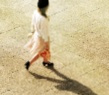
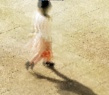
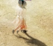
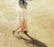
(a)	(b)	(b)	(b)	(b)

Figure 1: (a) Original still image. (b) Warps with different motion magnitude steps — obtained from predicted motion — overlaid over original image.

In human visual perception, expectation of what is going to happen next is essential for the on time interpretation of the scene and preparing for reaction when needed. The underlying idea in estimating motion patterns from a single image is illustrated by the walking person in figure 1. This figure is obtained from the proposed method by warping the static image with the predicted motion at different magnitude steps. For a human observer it is obvious what to expect in figure 1: motion in the legs and arms, while the torso moves to the right. From these clues we build our expectation. (That is the reason why the moonwalk by Michael Jackson is so salient as it refutes the expectation.) Closer inspection of figure 1 reveals that only the face, the legs and hands expose the expected motion direction, whereas the torso cannot reveal the difference to left or to the right. This indicates that motion is locally predictable. Therefore, for building motion expectation we start with local parts rather than the complete silhouette.

The paper shows that motion prediction in static images is possible by learning it from videos and transferring this knowledge to unseen static images. The proposed method does not use any localized object-class labels or frame-level annotations; it only requires suitable training videos. We consider a few applications of predicted motion: weak proposals of frames containing unexpected events, action recognition, motion saliency. This work has three main contributions: (i) a method for learning to predict motion in single static images from a training set of videos; (ii) to that end, extension of Structured Random Forests (SRF) with regression; (iii) a set of proposed possible applications for the motion prediction in single static images. Figure 2 illustrates the submitted approach.

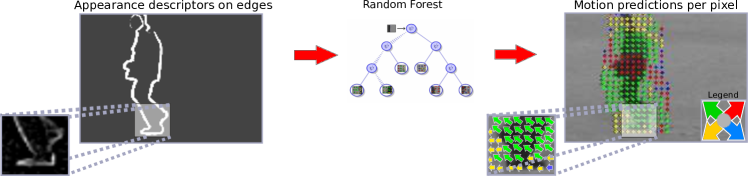
Figure 2: The Random Forest receives as input pairs of appearance-motion patches and learns the correlation from the part-based appearance to its corresponding motion.

2 Related Work

Adding motion to still images is also considered in SIFT flow [22], albeit with a different goal in mind — global image aligning for scene matching. As opposed to this work, in [22] two images are first aligned by matching local information and, subsequently, the motion from the training frame is transferred to the test frame. Other work visualizes motion in a static image by locally blurring along a vector field [3] or creates a motion sensation illusion by varying oriented image filters [12]. In [6] the authors learn affine motion models from the blurring information in the $\alpha$-channel, while [4] proposes a grouping of point trajectories based on different types of estimated camera motion. The authors of [16] focus on trajectory prediction by using scene information. Unlike these works, the proposed method predicts local motion by learning it from videos.

Local methods in video-based action recognition only depend on a pair of consecutive frames to compute the temporal derivative [10, 17] or optical flow [20, 31]. Because the temporal derivative lacks the motion direction and magnitude, this work focuses on predicting the more informative optical flow. Next to optical flow we also consider representing the motion as flow derivatives. These have been used in [7] for MBH (Motion Boundary Histograms) computation.

Cross-modal approaches use static images to recognize actions in videos [15] and appearance variations in videos to predict and localize objects in static images  [24]. Similarly, we propose a cross-modal approach: learning from videos and applying the learned model to static images.

Structured learning is suitable for this approach because motion is spatially correlated. Therefore, it is more appropriate to consider motion-patches, rather than look at pixel-wise motion vectors. Several structured learning approaches are available, such as CRF (Conditional Random Field) [19], Structured SVM (Support Vector Machines) [28] or Structured Random Forests [18]. In this paper we use an SRF (Structured Random Forest) because it has innate feature selection and allows for easy parallelization.

In [18], the authors use SRF for semantic segmentation. Here, each feature-patch has a corresponding patch of semantic labels instead of a single pixel label. In contrast to Kontschieder et al. [18], we predict motion in static images. Thus, we work with continuous data (regression) where the labels are patches of measured motion vectors, not discrete classes. Apart from solving different problems: motion prediction versus image segmentation, we also perform different learning tasks: regression (continuous motion vectors) versus classification (pixel-level class labels). The more recent work of Dollár et al. [9] proposes the use of SRF for edge detection. Rather than estimating joint probabilities for the edge-pixels — which would be prohibitively expensive — they map their structured space to a discrete unidimensional space on which they evaluate the goodness of each split. Contrary to [9], in this work the outputs are continuous motion vectors, thus mapping from patches of continuous vectors to a discrete space is not straightforwardly done and not without discarding useful information.

3 Motion Prediction — Formalism

Closer inspection of figure 2 reveals that the motion magnitude and direction are correlated with the appearance and they are consistent in a given neighborhood, therefore the problem requires structured output rather than single pixel-wise predictions. Thus, to learn motion from local appearance, this method uses a structured learning approach — SRF — which is fine tuned for regression.

A random forest is composed out of a number of trees. Each tree receives as input a set of training patches, $\mathcal{D}$, and their associated continuous motion patches — spatial derivatives of optical flow or optical flow, as in figure 3.a.

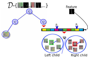
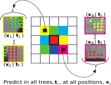
(a)	(b)

Figure 3: (a) Random Forest splitting: pixel-wise variance over the continuous motion vectors is estimated for all the training samples and all the splits. (b) Motion prediction in neighborhood: the neighbors of the current patch contribute to the final prediction at the current location due to overlap.

Node splitting. For each node in the tree, a number of splits $\Psi$, are generated by sampling: two random dimensions of the training features — $\mathbf{F}$, denoted by $p_{1}$ and $p_{2}$, a random threshold $t$ and a split type that is randomly picked out of the following four split types:

$$\Psi_{1} =\mathbf{F}(p_{1})\geq t\hskip 30.11249pt \hskip 30.11249pt\Psi_{3} =\mathbf{F}(p_{1})-\mathbf{F}(p_{2})\geq t$$ (1)

$$\Psi_{2} =\mathbf{F}(p_{1})+\mathbf{F}(p_{2})\geq t\hskip 30.11249pt \hskip 30.11249pt\Psi_{4} =\mid\mathbf{F}(p_{1})-\mathbf{F}(p_{2})\mid\geq t.$$ (2)

Each generated split, $\Psi$, is evaluated at every training sample in the set $\mathcal{D}$. This decides if the sample goes to the left child, containing the values larger than $t$ or to the right child with values lower than $t$.
Split Optimization. At each node, the best split — $\Psi^{*}$ — is retained. The quality of a split is often evaluated by an information gain criterion [1, 18]. Alternatively, [11] optimizes the splits by minimizing a problem-specific energy formulation. Unlike in the common RF problems, here the predictions are continuous optical flow/flow derivative. This entails an SRF regression — which is based on a motion similarity measure.

In [14], continuous predictions in the RF are approached by estimating the best split as the one corresponding to the smallest squared distance to the mean in each node. Despite its simplistic nature, the use of variance for regression in RF is also indicated as effective in practice in [5, 9]. In this case, the predictions are motion patches rather than single labels, which requires a measure of diversity of patterns inside these patches. For this purpose, we use pixel-wise variance:

$$\mathcal{V}_{\mathcal{S}_{\Psi}} =\sum_{\mathbf{x}\in{\mathcal{S}_{\Psi}}}\frac{1}{\mid P\mid}\sum_{i\in P}\frac{\sum_{j}^{D}(x_{i}^{j}-\mu_{i}^{j})^{2}}{\mid{\mathcal{S}_{\Psi}}\mid-1},$$ (3)

where $\mathcal{S}_{\Psi}\in\{\mathcal{L}_{\Psi},\mathcal{R}_{\Psi}\}$ is the left/right child node, $P$ is the set of pixels in a patch — $\mathbf{x}$, $D$ is the number of dimensions (i.e. the 2 flow components) and $\mu_{i}^{j}$ is the mean motion at pixel $i$ and dimension $j$.

Consequently, the best split is the one characterized by minimum variance of patch patterns inside the two generated children:

$$\Psi^{*} =\text{argmin}_{\Psi}\frac{\mathcal{V}_{\mathcal{L}_{\Psi}}\mid\mathcal{L}_{\Psi}\mid+\mathcal{V}_{\mathcal{R}_{\Psi}}\mid\mathcal{R}_{\Psi}\mid}{\mid\mathcal{L}_{\Psi}\mid+\mid\mathcal{R}_{\Psi}\mid},$$ (4)

where $\mathcal{V}_{\mathcal{L}_{\Psi}/\mathcal{R}_{\Psi}}$ are the variances of the two child nodes (eq. 3). The weighting by the node sizes is regularly used in RF to encourage more balanced splits [18].
Edge features. The features used are patch-based HOG descriptors extracted over the opponent color space [29]. Given that motion can only be perceived at textured edge-patches (the aperture problem), we make the choice of extracting training patches for the SRF along the edges. This reduces the number of samples by retaining the relevant ones in terms of motion perception.
Worst-first tree growing. For stopping the tree growing and deciding to create a leaf, it is customary to threshold the variance (defined in eq. 3) [1, 5, 18]. Rather than deciding to stop only based on variance thresholds, which can be cumbersome for different classes: i.e. classes with larger motion magnitudes such as running or jogging have inherently higher motion variance than classes such as boxing, we can impose a limit on the number of leaves we want in each tree.

[26] proposes the use of directed graphs for decision making. These graphs are iteratively optimized by alternating between finding the best splitting function and finding the best child assignment to parent nodes. Unlike here, the proposed “worst-first” tree growing changes the order in which the nodes are visited, but not the topology of the trees. At each timestep the worst node — with the highest variance as defined in equation 3 — is chosen to be split next. Finally, when the number of terminal nodes reaches the number of desired leaves, the splitting process ends and all terminal nodes are transformed into leaves.

By following this procedure we ensure that the more diverse nodes are split first, thus allowing for a fairly balanced tree at stopping time — when the desired number of leaves is reached. Given that the data is more evenly split, this can be seen as a measure against overfitting as well as a speedup.
Leaf patch. A leaf is created when all the patches in one node have a similar pattern. To enforce this, one can threshold the variance measure defined in equation 3 or additionally, as discussed above, grow the trees in a worst-first manner and select a desired number of leaves. At the point when a leaf node is created, it contains a set of patches, that are assumed to have a uniform appearance. Thus, we define the leaf prediction as the average over the patches in the node. This is a common approach for regression RF [5, 14] and, despite its simplicity, proves effective in practice.
Motion Prediction. Given an input test appearance patch, the goal is to obtain a motion prediction, $\textbf{x}^{*}$, from the trained SRF. For this, the method first evaluates at each edge-pixel in the image the most likely prediction over the trees of the SRF. Following the approach of [5, 14] we define the prediction over trees as the average patch: $\mathbf{x}^{*}=\frac{1}{\mid\mathcal{T}\mid}\sum_{\mathbf{x}\in\mathcal{T}}\mathbf{x}$, where $\mathcal{T}$ is the set of tree predictions at the current position. At last, because the patches overlap as shown in figure 3.b, the final prediction at each pixel position is the average over all overlapping predictions at that position.

4 Motion Prediction — Learning and Features

SRF patch size selection. All experiments use the same patch size for features and for motion. Figures 4.a and 4.b show that a small patch size would fail to provide an indication for the expected motion direction. On the other hand, large patch sizes would be prone to prediction mistakes since full-body poses are characterized by larger motion diversity, thus, harder to learn than local patches. We have experimented with different patch sizes, and found a patch size approximately 5 times smaller than the maximum image size to be reasonable.

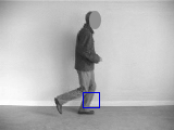
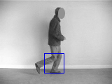
(a) Patch $11\times 11$	(b) Patch $32\times 32$	(c) Original flow	(d) Corrected flow

Figure 4: (a) & (b) Patch size selection: small patch sizes fail to capture motion direction, while large ones are more error prone. (c) & (d) Camera motion correction — section 6.3: (c) original Farnebäck flow estimation, (d) affine corrected flow estimation.

Training features and labels. The model learns motion from static appearance features at Canny edges to avoid the aperture problem. Motion is represented by dense optical flow, and optical flow derivatives respectively, measured at every pixel in the patch. For flow estimation we use the OpenCV library. One opponent-HOG descriptor is extracted over each training patch. Each HOG computation uses 2$\times$2 spatial bins, 9 orientations and has 3 color-channels.
SRF parameter settings. The SRF uses 50 iterations per node during training and another 10 for finding the optimal threshold (eq. 2). Given that the patch-features have 108 dimensions, the number of iterations — usually set to the square root of the number of feature dimensions — is sufficient. All trees are grown in the “worst-first” manner until a number of 1,000 leaves is reached, additionally leaves are created when the variance (eq. 3) goes below a 0.1 threshold. Each tree in the SRF is trained on 20 random pairs of sequential frames.

5 Evaluating Motion Prediction

This section focuses on evaluating the SRF motion predictions with respect to measured and ground truth video motion. The goal of this experiment is to test the ability to learn motion from appearance. For evaluation, we use both KTH [25] and Sintel [2] datasets. The choice for the simplistic KTH dataset is motivated by its laboratory setting providing limited appearance variations and reliable optical flow measurements — limited to no camera motion.

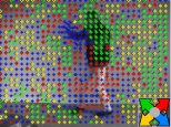
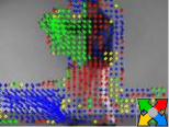
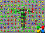
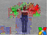
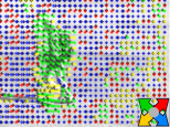
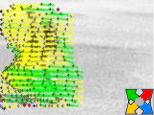
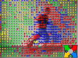
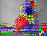
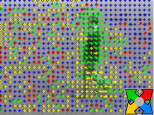
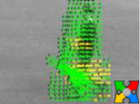
(a)	(b)	(c)	(d)	(e)

Figure 5: (a) Original image. (b) Measured optical flow vectors. (c) Predicted optical flow vectors. (d) Measured flow map. (e) Flow map of the predictions (colors as in [23]).

Setup. We use the KTH dataset where the data is split in the standard manner [25]. From each video we retain only a set of 20 sequential frames. We compare the motion predictions against measured flow on the complete data — trainval and test. For each one of the 6 classes we train an SRF regressor containing 11 trees. We train SRFs on the training set and use them to predict on the validation set and vice versa. Finally, we merge the SRFs of the two sets and use them for predicting on the test. Given that we extract motion patches along the Canny edges, we evaluate the motion predictions at the edge points. We use the standard optical flow error estimation — EPE (End-Point-Error) — which computes the Euclidian distance between the end point of the measured OF and the predicted one. We also evaluate the direction of predicted flow by computing the cosine similarity between the prediction and the measurement: $\frac{x_{1}x_{2}+y_{1}y_{2}}{\sqrt{x_{1}^{2}+y_{1}^{2}}\sqrt{x_{2}^{2}+y_{2}^{2}}}$. The orientation of the flow is estimated as the angle between the prediction and the measured OF on the half-circle: $\frac{\mid x_{1}x_{2}+y_{1}y_{2}\mid}{\sqrt{x_{1}^{2}+y_{1}^{2}}\sqrt{x_{2}^{2}+y_{2}^{2}}}$.

	Edge EPE	0-Edge EPE	Edge direction	Edge orientation
Boxing	1.23 px	1.21 px	3.86 %	66.60 %
Clapping	1.13 px	1.08 px	1.18 %	65.80 %
Waving	1.65 px	1.59 px	-0.49 %	67.52 %
Jogging	4.51 px	4.61 px	14.39 %	76.52 %
Running	8.41 px	8.62 px	26.68 %	77.02 %
Walking	3.90 px	3.92 px	10.80 %	72.17 %
Avg.	3.47 px	3.50 px	9.40 %	70.94 %

Table 1: Predicted EPE (End-Point-Error) at the Canny edges compared to the EPE of the zero prediction. Cosine similarity at edge-points for direction estimation. Cosine similarity at edge-points using the angle on the half-circle for orientation estimation. The direction and orientation should be as close as possible to 100%.

Evaluation. Figure 5 depicts a few examples of measured motion comparative to predicted motion and their corresponding flow maps. Noteworthy here is that the predicted motion is realistic and in agreement with the expectation of the observer. Moreover, the flow maps for the measured flow are similar to the flow maps of the predicted motion. Table 1 shows that for jogging, running and walking the EPEs are lower than the 0-prediction and also on average the predicted motion is better than the 0-EPE. While looking at the direction estimation, one can see that the first 3 classes are quite often wrong — due to the characteristic bidirectional motion. On the other hand, the orientation of the flow is considerably better (closer to 100%) especially for the last 3 classes that involve larger motion magnitudes — jogging, running and walking.

	Edge EPE	0-Edge EPE	Edge direction	Edge orientation
Horn-Schunck	4.25 px	4.21 px	02.72 %	65.69 %
Lucas-Kanade	3.18 px	3.22 px	08.30 %	70.03 %
Farnebäck	3.47 px	3.50 px	09.40 %	70.94 %
Simple Flow	0.91 px	1.01 px	18.30 %	70.08 %

Table 2: Average scores over classes at the Canny edges compared to the scores of the zero prediction when the training of the SRFs uses different flow algorithms: Farnebäck, Horn-Schunck, Lucas-Kanade, Simple Flow.

Impact of flow algorithm. Table 2 shows the average scores over the classes when the training of the SRFs is based on different existing flow algorithms. Farnebäck and Simple Flow are characterized by smaller errors in both flow magnitude as well as flow direction and orientation — Simple Flow has a 10% relative gain over the 0-baseline in magnitude while Farnebäck gains a 3% over the 0-baseline. Yet the direction of the prediction is more often correct when training on Farnebäck flow.

We run an additional experiment on the Sintel dataset [2] for which ground truth flow is provided. We have retained 10 frames out each training video for learning the SRF and used the rest for testing. We have trained only one SRF containing 11 trees where each tree was trained on maximum 20 randomly sampled frame pairs. We have compared the predictions of the SRF when using the ground truth flow with the measured flow for both Simple Flow and Farnebäck. The scores are computed with respect to the ground truth flow. Table 3 displays the results. Predicted flow outperforms Farnebäck measurements in terms of edge EPE, while the direction of the predicted flow is often correct.

	SRF prediction	Simple Flow	Farnebäck
Edge EPE	11.46 px	09.26 px	14.42 px
Edge direction	38.64 %	71.18 %	71.26 %
Edge orientation	73.45 %	80.88 %	84.63 %

Table 3: Average scores over classes on Sintel data estimated at Canny edges. The measured Farnebäck and Simple Flow are compared to the SRF predictions.

Comparison with other learning methods. Table 4 compares the SRF motion predictions on the KTH data with motion predictions obtained by training a pixel-wise SVR (Support Vector Regressor) with linear kernel and pixel-wise least squares regression. We train a separate regressor for the x and y coordinates of the flow. The SRF obtains the smallest error — 3% relative gain over the 0 baseline while the other two methods perform worse than the 0-baseline. This experiment ascertains the need for a structured learning regression method.

	0-prediction	SRF	SVR	Least squares
Edge EPE	3.50 px	3.47 px	5.02 px	6.09 px

Table 4: Average EPE over classes on KTH data estimated at Canny edges when all methods are trained on Farnebäck flow.

6 Applications of Motion Prediction

In this section, we bring forth a few possible uses of the predicted motion. One could consider other applications, as this is not a complete list of tasks that could benefit from motion prediction. Application 1 gives an illustration of weakly detecting unexpected events in videos. Application 2 evaluates how far off is the predicted motion from the measured motion in the context of action recognition. Application 3 focuses on the gain of adding motion prediction to action recognition in still images, while application 4 proposes a method for motion saliency in static images.

6.1 Application 1 — Illustration of finding unexpected events

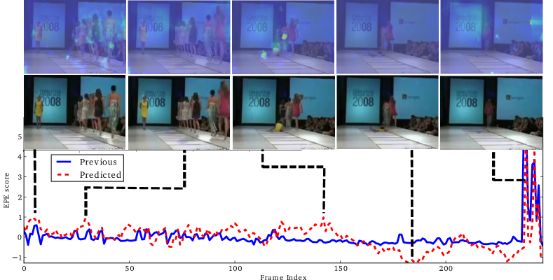
Figure 6: EPE between measured flow at previous frame and current frame in blue. EPE between measured flow at current frame and predicted flow at current frame in red. The two graphs are centered on 0 for illustration purpose. Images containing unexpected motion together with their associated EPE heatmaps are displayed on top.

This application shows a possible use of the motion prediction — finding unexpected events. We do not present this as an end goal of the proposed motion prediction method, but rather as an illustration of its usefulness. Given an SRF trained on a set of videos, one could use the SRF to obtain motion predictions at each frame in a given unseen video. If the EPE between the measured motion vectors and the predicted ones is large, it can be assumed that a motion that has not been seen before in the training data occurs at some point in the video.
Setup. For speed considerations, the SRF uses 3 trees. The training videos are queried from the TRECVid (TREC Video Retrieval Evaluation) [27, 30] development set. The frames are resized to maximum 300 px. We obtain motion predictions at each frame in the test video and compute the EPE score between the measured Farnebäck optical flow and the predicted flow. We retain the frames whose EPE scores are over one standard deviation from the mean. The same procedure is repeated for the baseline comparison, but this time by computing the EPE between the motion at the previous frame and the current frame.
Evaluation. Figure 6 displays the EPE error over the video frames, with respect to both previous frame and predicted motion. Frames containing interesting motion are displayed together with their corresponding EPE heatmaps. The video contains a catwalk show during which one person falls through the floor — unexpected event. Noteworthy is that the predicted motion graph is reasonably similar to the one based on the errors to the previous frame, while better emphasizing the interesting moments — when the person falls or is no longer visible in the frame — through the graph peaks.

6.2 Application 2 — Predicted vs. measured motion for AR

Being able to predict motion can provide useful information in the action recognition context. The predictions obtained from appearance can be combined with appearance features in an action recognition pipeline. We present this application from a compelling theoretical perspective as we are not interested in absolute numbers but in gaining insight about the feasibility of motion prediction and its relative usefulness when compared to measured motion.
Setup. We evaluate on the same KTH datatset. For action recognition, we follow the setting of Laptev et al. [20]. We extract HOG features for appearance description, and HOF, MBH respectively for motion description at Canny edges. We also use a level-2 spatial pyramid for all descriptors [21]. For each class we train a one-vs-all SVM classifier with HIK (Histogram Intersection Kernel) where the $C$ parameter is set by performing 5-fold crossvalidation on the subsampled trainval set. The obtained predictions from all 6 one-vs-all SVMs are ranked.

	HOG	Predicted Motion				Measured motion
		pHOF	HOG+ pHOF	pMBH	HOG+ pMBH	mHOF	mMBH
Boxing	0.58	0.56	0.58	0.61	0.70	0.75	0.78
Clapping	0.83	0.64	0.89	0.87	0.92	0.89	0.89
Waving	0.97	0.89	0.97	0.86	0.94	1.00	0.94
Jogging	0.72	0.61	0.78	0.56	0.70	0.78	0.81
Running	0.83	0.83	0.89	0.86	0.89	0.81	0.86
Walking	0.97	0.97	1.00	0.80	0.91	0.89	0.97
Avg.	0.82	0.75	0.85	0.76	0.84	0.85	0.88

Table 5: Action Recognition accuracy on the KTH dataset for HOG only, predicted/measured HOF — pHOF/mHOF — and predicted/measured MBH — pMBH/mMBH. The underlined text shows where the prediction results are better than static (HOG) while the bold shows the best.

Evaluation. Figure 5 shows a few examples of measured motion compared to predicted motion on KTH data, together with their corresponding flow maps. The accuracies for action recognition are displayed in table 5. The scores are lower than standarly reported in the literature due to the fact that we only use 20 frames per video. Here we compare the static features (HOG) with the combination of HOG and predicted motion (HOF and MBH). The measured motion exceeds the predicted motion in itself, but in combination with the appearance, the predicted motion can actually reach the scores of the measured motion. As expected, adding the motion information improves for categories that involve a larger amount of motion such as: running, jogging and walking and less so for boxing, handclapping and handwaving. It is worth noting that the combination of predicted HOF and HOG equals the measured HOF for this dataset. This proves that motion, even imperfect, brings useful information.

6.3 Application 3 — Predicted motion for AR in Still Images

While application 2 estimates how far apart are the predicted motion and the measured motion in the context of action recognition, here we predict motion over inherently static images which lack the video compression artifacts or motion blurring. The models are trained on realistic video-data and this application analyzes if the learned motion can, indeed, be transferred to still images. We measure the value of the static motion predictions in the context of image-based action recognition. Again, the goal here is to test the ability of predicting motion and its added value, and less so to improve over state-of-the-art.

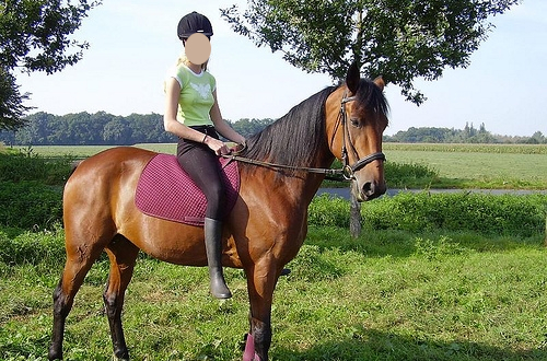
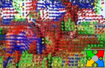
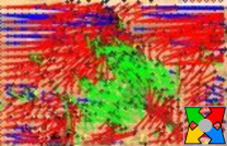
(a)	(b)	(c)	(d)

Figure 7: (a) Examples of images from the static Willow dataset  [8]. (b) Warped image using the predicted motion, overlaid over the original image. (c) Predicted flow vectors. (c) The training appearance associated in the SRF with the predictions. More examples of static images animated with predicted motion can be found at: http://silvialaurapintea.github.io/dejavu.html.

Setup. We apply the motion predictions on a static action recognition dataset — Willow [8]. For each class we train a separate SRF on TRECVid data as in application 1. For each image we obtain seven flow/flow derivative predictions — one per class, subsequently used for HOF/MBH descriptor extraction. In the action recognition part we use the same setting as in application 2, except that we extract descriptors densely over the images.
Affine camera motion correction. The videos used for training SRFs are realistic videos characterized by large camera motion which drastically affects the Farnebäck measurements. To correct for camera motion we assume an affine motion model whose parameters we determine by first selecting a set of interest points in the two sequential frames. These interest points are matched between frames and the consistent matches are retained by employing RANSAC. From the kept point-matches we estimated the parameters of the affine model. Given the affine camera motion estimation, we then correct the second frame for this motion and subsequently perform flow estimation. Figures 4.c and 4.d show an example of original flow estimation and camera-motion corrected flow.
Evaluation. Figure 7 displays a few examples from the static dataset together with their predicted motion vectors, the appearance associated in the SRF with that motion and the static image warped with the predicted motion overlaid on top of the original image. Interesting to notice in figure 7 is that the SRF manages to distinguish the foreground motion from the background motion. We notice here, that unlike in the case of KTH predictions (figure 5), there is predicted background flow, but this flow has at all times a different direction from the foreground motion.

The results of Delaitre et al. [8] (0.63 MAP) exceed the proposed motion prediction results due to the more sophisticated model and more fine-tuned features. Provided that we would process our features — HOG and HOF/MBH descriptors — in the manner described in [8], the relative improvement should remain. Despite the drawbacks of noisy motion estimations (i.e. figures 4.c and 4.d), low video quality as well as large camera motion, the SRFs are capable of learning the motion patterns characteristic for each class. By adding predicted HOF to the static HOG descriptors we obtain a relative gain of 1% in MAP – from 50% to 51% — and a 2% relative gain in accuracy.

6.4 Application 4 — Motion saliency

Motion saliency is yet another possible use for the predicted motion. Objects that move differently from their background are salient and capture the viewer’s attention. Being able to predict motion in static images provides the advantage of finding pixels that can be distinguished from their surrounding pixels through their motion. Inspired by [13], we propose descriptor pooling based on predicted flow. Rather than pooling image descriptors on spatial location only, here we also pool them on their predicted motion.

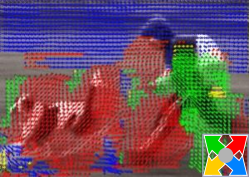
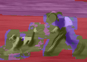
(a)	(b)	(c)

Figure 8: (a) Original still image. (b) Predicted flow vectors in the still image. (c) Grouping descriptors based on their predicted motion — each color represents a pool in the flow-based spatial pyramid.

Setup. This application uses the same experimental setup as application 3. We add to the spatial pyramid 10 more pools based on the predicted motion: 4 pools for the quadrants of the flow angles, 1 pool for the 0 prediction times 2 pools for flow magnitude larger/equal to 0.
Evaluation. Figure 8 displays an example of a static image together with its associated predicted motion vectors from the SRF and the corresponding motion grouping in the motion-based pooling framework. We notice that the background is grouped into a different pool than the foreground and also the pixels associated with the dog are grouped together while the ones corresponding to the boy are organized into a separate group.

By adding motion based pooling to static images, we obtain a 1% relative improvement in both MAP and accuracy over the results in application 3. Thus, overall we have a relative gain on 2% in MAP and 3% in accuracy over static HOG features by adding motion — predicted HOF features and flow-based pooling. Adding the flow-based pooling leads to improvements especially for the classes that involve a larger amount of motion: riding bike, riding horse and walking. The outcome of this application ascertains that grouping pixels that have similar motion brings conclusive information.

7 Discussion

The experimental evaluation tests the ability of the proposed method to learn motion given appearance features. One limitation of the method is data dependency — the learned motion depends on the quality of the training data and its similarity to the test data. This can be observed in application 3 where motion is learned from complex realistic videos characterized by noise, motion blur and camera motion, yet the predictions are tested on high quality static images. Another drawback is the class dependency — each action class is characterized by a certain direction and magnitude in the motion of the part (i.e. arms, legs) and the SRFs learn class specific motion (figure 5). Nonetheless, the considered applications show that learning motion from appearance is possible. Finally, the SRF code is made available online at: http://silvialaurapintea.github.io/dejavu.html.

8 Conclusions

This paper proposes a method for motion prediction based on structured regression with RF. The undertaken task of performing structured regression in Random Forest is novel, as well as the problem of learning to predict motion in still images. We experimentally provide an answer to our first research question: can we learn to predict motion from appearance only? And we prove that this is possible provided proper training data and reliable optical flow estimates. Furthermore, for illustrative purposes, we apply the proposed motion prediction method to a set of tasks and validate that the predicted, imperfect, motion adds novel and useful information over the static appearance features only, which answers our second research question. Finally, motion prediction can be employed in a multitude of topics such as: action anticipation or conflict detection. Another possible use for motion prediction is camera motion removal — if the training videos are characterized by camera motion, the SRF is bound to learn the distinction between foreground and background motion (fig. 7, 8).
Acknowledgements.
This research is supported by the Dutch national program COMMIT.

References

- [1] Breiman, L.: Random forests. In: Machine learning (2001)
- [2] Butler, D.J., Wulff, J., Stanley, G.B., Black, M.J.: A naturalistic open source movie for optical flow evaluation. In: ECCV (2012)
- [3] Cabral, B., Leedom, L.C.: Imaging vector fields using line integral convolution. In: Computer graphics and interactive techniques (1993)
- [4] Cifuentes, C.G., Sturzel, M., Jurie, F., Brostow, G.J., et al.: Motion models that only work sometimes. In: BMVC (2012)
- [5] Criminisi, A., Shotton, J., Konukoglu, E.: Decision forests: A unified framework for classification, regression, density estimation, manifold learning and semi-supervised learning. In: Foundations and Trends® in Computer Graphics and Vision (2012)
- [6] Dai, S., Wu, Y.: Motion from blur. In: CVPR (2008)
- [7] Dalal, N., Triggs, B., Schmid, C.: Human detection using oriented histograms of flow and appearance. In: ECCV (2006)
- [8] Delaitre, V., Laptev, I., Sivic, J.: Recognizing human actions in still images: a study of bag-of-features and part-based representations. In: BMVC (2010)
- [9] Dollár, P., Zitnick, C.L.: Structured forests for fast edge detection. In: ICCV (2013)
- [10] Everts, I., van Gemert, J., Gevers, T.: Evaluation of color stips for human action recognition. In: CVPR (2013)
- [11] Fanello, S., Keskin, C., Kohli, P., Izadi, S., Shotton, J., Criminisi, A., Pattaccini, U., Paek, T.: Filter forests for learning data-dependent convolutional kernels
- [12] Freeman, W.T., Adelson, E.H., Heeger, D.J.: Motion without movement. In: Computer Graphics (1991)
- [13] van Gemert, J.: Exploiting photographic style for category-level image classification by generalizing the spatial pyramid. In: ICMR (2011)
- [14] Hastie, T., Tibshirani, R., Friedman, J.J.H.: The elements of statistical learning (2001)
- [15] Ikizler-Cinbis, N., Cinbis, R., Sclaroff, S.: Learning actions from the web. In: ICCV (2009)
- [16] Kitani, K.M., Ziebart, B.D., Bagnell, J.A., Hebert, M.: Activity forecasting. In: ECCV (2012)
- [17] Klaser, A., Marszałek, M., Schmid, C., et al.: A spatio-temporal descriptor based on 3d-gradients. In: BMVC (2008)
- [18] Kontschieder, P., Rota Bulò, S., Bischof, H., Pelillo, M.: Structured class-labels in random forests for semantic image labeling. In: ICCV (2011)
- [19] Lafferty, J., McCallum, A., Pereira, F.: Conditional random fields: probabilistic models for segmenting and labeling sequence data. In: ICML (2001)
- [20] Laptev, I., Marszalek, M., Schmid, C., Rozenfeld, B.: Learning realistic human actions from movies. In: CVPR (2008)
- [21] Lazebnik, S., Schmid, C., Ponce, J.: Beyond bags of features: Spatial pyramid matching for recognizing natural scene categories. In: CVPR (2006)
- [22] Liu, C., Yuen, J., Torralba, A., Sivic, J., Freeman, W.: Sift flow: Dense correspondence across different scenes. In: ECCV (2008)
- [23] Max, N., Crawfis, R., Grant, C.: Visualizing 3d velocity fields near contour surfaces. In: Conference on Visualization (1994)
- [24] Prest, A., Leistner, C., Civera, J., Schmid, C., Ferrari, V.: Learning object class detectors from weakly annotated video. In: CVPR (2012)
- [25] Schuldt, C., Laptev, I., Caputo, B.: Recognizing human actions: a local svm approach. In: ICPR (2004)
- [26] Shotton, J., Sharp, T., Kohli, P., Nowozin, S., Winn, J., Criminisi, A.: Decision jungles: Compact and rich models for classification. In: NIPS (2013)
- [27] Smeaton, A., Over, P., Kraaij, W.: Evaluation campaigns and trecvid. In: ACM-mir (2006)
- [28] Tsochantaridis, I., Joachims, T., Hofmann, T., Altun, Y., Singer, Y.: Large margin methods for structured and interdependent output variables. In: JMLR (2006)
- [29] Van De Sande, K.E., Gevers, T., Snoek, C.G.: Evaluating color descriptors for object and scene recognition. In: PAMI (2010)
- [30] Van Gemert, J.C., Veenman, C.J., Geusebroek, J.M.: Episode-constrained cross-validation in video concept retrieval. Transactions on Multimedia (2009)
- [31] Wang, H., Ulla, M.M., Klaser, A., Laptev, I., Schmid, C.: Evaluation of local spatio-temporal features for action recognition. In: BMVC (2009)