The Cohomology for Wu Characteristics

Abstract.

While the Euler characteristic $\chi(G)=\omega_{1}(G)=\sum_{x}\omega(x)$ super counts simplices, the Wu characteristics $\omega_{k}(G)=\sum_{x_{1}\sim x_{2}\dots\sim x_{k}}\omega(x_{1})\cdots\omega(x_{k})$ super counts simultaneously pairwise interacting $k$-tuples of simplices in a finite abstract simplicial complex $G$. More generally, one can define the $k$-intersection number $\omega_{k}(G_{1},\dots G_{k})$, which is the same sum but where $x_{i}\in G_{i}$. For every $k\geq 1$ we define a cohomology $H^{p}_{k}(G_{1},\dots,G_{k})$ compatible with $\omega_{k}$. It is invariant under Barycentric subdivison. This interaction cohomology allows to distinguish spaces which simplicial cohomology can not: for $k=2$, it can identify algebraically the Möbius strip and the cylinder. The vector spaces $H^{p}_{k}(G)$ are defined by explicit exterior derivatives $d_{k}$ which generalize the incidence matrices for simplicial cohomology. The cohomology satisfies the Kuenneth formula: for every $k$, the Poincaré polynomials $p_{k}(t)$ are ring homomorphisms from the strong ring to the ring of polynomials in $t$. The case $k=1$ for Euler characteristic is the familiar simplicial cohomology $H^{p}_{1}(G)=H^{p}(G)$. On any interaction level $k$, there is now a Dirac operator $D=d_{k}+d_{k}^{*}$. The block diagonal Laplacian $L=D^{2}$ leads to the generalized Hodge correspondence $b_{p}(G)={\rm dim}(H^{p}_{k}(G))={\rm dim}({\rm ker}(L_{p}))$ and Euler-Poincaré $\omega_{k}(G)=\sum_{p}(-1)^{p}{\rm dim}(H^{p}_{k}(G))$ for Wu characteristic and more generally $\omega_{k}(G_{1},\dots G_{k})=\sum_{p}(-1)^{p}{\rm dim}(H^{p}_{k}(G_{1},\dots,G_{k}))$. Also, like for traditional simplicial cohomology, an isospectral Lax deformation $\dot{D}=[B(D),D]$, with $B(t)=d(t)-d^{*}(t)-ib(t)$, $D(t)=d(t)+d(t)^{*}+b(t)$ can deform the exterior derivative $d$ which belongs to the interaction cohomology. Also the Brouwer-Lefschetz fixed point theorem generalizes to all Wu characteristics: given an endomorphism $T$ of $G$, the super trace of its induced map on k’th cohomology defines a Lefschetz number $L_{k}(T)$. The Brouwer index $i_{T,k}(x_{1},\dots,x_{k})=\prod_{j=1}^{k}\omega(x_{j}){\rm sign}(T|x_{j})$ attached to simplex tuple which is invariant under $T$ leads to the formula $L_{k}(T)=\sum_{T(x)=x}i_{T,k}(x)$. For $T=Id$, the Lefschetz number $L_{k}(Id)$ is equal to the $k$’th Wu characteristic $\omega_{k}(G)$ of the graph $G$ and the Lefschetz formula reduces to the Euler-Poincaré formula for Wu characteristic. Also this generalizes to the case, where automorphisms $T_{k}$ act on $G_{k}$: there is a Lefschetz number $L_{k}(T_{1},\dots,T_{k})$ and indices $\prod_{j=1}^{k}\omega(x_{j}){\rm sign}(T_{j}|x_{j})$. For $k=1$, it is the known Lefschetz formula for Euler characteristic. While Gauss-Bonnet for $\omega_{k}$ can be seen as a particular case of a discrete Atiyah-Singer result, the Lefschetz formula is an particular case of a discrete Atiyah-Bott result. But unlike for Euler characteristic $k=1$, the elliptic differential complexes for $k>1$ are not yet associated to any constructions in the continuum.

1. Introduction

1.1.

An abstract finite simplicial complex $G$ is a finite set of non-empty subsets that is closed under the process of taking non-empty subsets. It defines a new complex $G_{1}$, where $G_{1}$ is the set of subsets of the power set $2^{G}$ which are pairwise contained in each other. This is called the Barycentric refinement of $G$. Quantities which do not change under Barycentric refinements are combinatorial invariants [2]. Examples of such quantities are the Euler characteristic, the Wu characteristics [35, 21] or Green function values [26]. An important class of complexes are Whitney complexes of a finite simple graph in which $G$ consists of all non-empty subsets of the vertex set, in which all elements are connected to each other. A Barycentric refinement $G_{1}$ of a complex $G$ is always a Whitney complex. The graph has the sets of $G$ as vertices and connects two if one is contained in the other.

1.2.

While Euler characteristic $\chi(G)=\sum_{x}\omega(x)$ super counts the self interactions of simplices within the geometry, the Wu characteristic $\omega_{k}$ super counts the intersections of $k$ different simplices

$$\omega_{k}(G)=\sum_{x_{1}\sim\dots\sim x_{k}}\omega(x_{1})\cdots\omega(x_{k})\;,$$

where $x_{1}\sim\dots\sim x_{k}$ means that $(x_{1},x_{2},\cdots x_{k})\in G^{k}=G\times G\times\cdots\times G$ all pairwise intersect. While originally introduced for polytopes by Wu in 1959, we use it for simplicial complexes and in particular for Whitney complexes of graphs. Especially important is the quadratic case

$$\sum_{x\sim y}\omega(x)\omega(y)$$

which produces an Ising type nearest neighborhood functional if we think of even or odd dimensional simplices as spins of a two-state statistical mechanics system. We call the cohomology for Wu characteristic an interaction cohomology because the name ”intersection cohomology” is usedin the continuum for a cohomology theory by Goresky-MacPherson.

1.3.

As in [21], where we proved Gauss-Bonnet, Poincaré-Hopf, and product formulas for Wu characteristics in the case of Whitney complexes, we can work in the slightly more general frame work of finite abstract simplicial complexes. If we look at set of subsets of $G\times G\cdots\times G$ of a simplicial complex $G$ such that all $k$ elements pairwise intersect, we obtain a $k$-intersection complex. For $k=1$ the complex is $G$ itself, the connection-oblivious complex. For $k=2$ the intersection relations give the interaction graph $G^{\prime}$ which was studied in [22, 28, 27, 23, 25, 26]. It contains the Barycentric refinement graph $G_{1}$. For every $k>1$ we get an example of an “ordinary cohomology” generalizing the simplicial cohomology.

1.4.

A major reason to study the Wu characteristic, is that each $\omega_{k}$ is multiplicative with respect to the graph product [19] $G,H\to(G\times H)_{1}$, in which the pairs $(x,y)$ are vertices with $x\in G$ and $y\in H$ and where two vertices are connected if one is contained in the other. It is already multiplicative with respect to the Cartesian product $G\times H$, which unlike $(G\times H)_{1}$ is not a simplicial complex any more. The multiplicative property makes the $\omega_{k}$ functionals a natural counting tool, en par with Euler characteristic $\chi(G)=\omega_{1}(G)$, which is the special case $k=1$. The corresponding cohomologies belong to a generalized calculus which does not yet seem to exist in the continuum. The multiplicative property of the functionals is especially natural when looking at the Cartesian product $G\times H$ in the strong ring generated by simplicial complexes in which the simplicial complexes are the multiplicative primes and where the objects are signed to have an additive group. The subring of zero-dimensional complexes can be identified with the ring of integers.

1.5.

Traditionally, graphs are seen as zero-dimensional simplicial complexes. A more generous point of view is to see a graph $G=(V,E)$ as a structure on which simplicial complexes can live, similarly as topologies, sheaves or $\sigma$-algebras are placed on sets. The $1$-dimensional complex $V\cup E$ is only one of the possible simplicial complexes. An other example is the graphic matroid defined by trees in the graph. But the most important complex imposed on a graph is the Whitney complex. It is defined by the set of complete subgraphs of $G$. Without specifying further, we always associate a graph equipped with its Whitney complex.

1.6.

The class of all finite simple graphs $G=(V,E)$ is a distributive Boolean lattice with union $(V_{1}\cup V_{2},E_{1}\cup E_{2})$ and intersection $(V_{1}\cap V_{2},E_{1}\cap E_{2})$. The same is true for finite abstract simplicial complexes, where also the union and intersection remain both simplicial complexes. But unlike the Boolean lattice of sets, the Boolean lattices of graphs or complexes are each not a ring: the set theoretical addition $G\Delta H=G\cup H\setminus G\cap H$ is in general only in the larger category of chains. But if we take the disjoint union of graphs as ”addition” and the Cartesian multiplication of sets as multiplication, we get a ring [27].

1.7.

All of the Wu characteristics $\omega_{k}$ are functions on this ring. They are of fundamental importance because they are not only additive $\omega_{k}(A\dot{\cup}B)=\omega_{k}(A)+\omega_{k}(B)$ but also multiplicative $\omega_{k}(A\times B)=\omega_{k}(A)\omega_{k}(B)$. In other words, all the Wu characteristic numbers $\omega_{k}$ and especially the Euler characteristics $\chi=\omega_{1}$ are ring homomorphisms from the strong ring to the integers. This algebraic property already makes the Wu characteristics important quantities to study.

1.8.

Euler characteristic is distinguished in having additionally the property of being invariant under homotopy transformations. It is unique among linear valuations with this property. The lack of homotopy invariance for the Wu characteristic numbers for $k\geq 2$ is not a handicap, in contrary: it allows for finer invariants: while for all trees for example, the Euler characteristic is $1$, the Wu characteristic $\omega(G)=\omega_{2}(G)$ is more interesting: it is $\omega(G)=5-4n+M(G)$, where $n=\sum_{v\in V}1$ is the vertex cardinality and $M$ is the Zagreb index $M(G)=\sum_{v}{\rm deg}(v)^{2}$. This tree formula relating the Wu characteristic with the Zagreb index has been pointed out to us by Tamas Reti.

1.9.

There are other natural operations on simplicial complexes. One is the Zykov addition which is in the continuum known as the join. Take the disjoint union $G,H$ of the graphs and additionally connect any pair of vertices from different graphs. The generating function $f_{G}(x)=1+\sum_{k=0}v_{k}x^{k+1}$ satisfies $f_{G+H}(x)=f_{G}(x)f_{H}(x)$ and $\chi(G)=1-f_{G}(-1)$ from which one can deduce that $i(G)=1-\chi(G)$ is multiplicative: $i(G+H)=i(G)i(H)$. Evaluating $f$ at $x=1$ instead shows that the total number of simplices $f_{G}(x)-1=\sum_{k}v_{k}$ is multiplicative. We don’t use the join much here.

1.10.

Looking at finite abstract simplicial complexes modulo Barycentric refinements already captures some kind topology. But Barycentric refinements are still rather rigid and do not include all notions of topology in which one wants to have a sense of rubber geometry. One especially wants to have dimension preserved. We introduced therefore a notion of homeomorphism in [17]. It uses both homotopy and dimension. The Barycentric refinement of a graph $G$ is homeomorphic to $G$ in that notion. This notion of homeomorphism could be ported over to simplicial complexes because the Barycentric refinement of an abstract simplicial complex is a Whitney complex of a graph. From a topological perspective there is no loss of generality by looking at graphs rather than simplicial complexes. We believe that the interaction cohomology considered here is the same for homeomorphic graphs but this is not yet proven.

1.11.

As topological spaces come in various forms, notably manifolds or varieties, one can also define classes of simplicial complexes or classes of graphs. In the continuum, one has historically started to investigate first very regular structures like Euclidean spaces, surfaces, then introduced manifolds, varieties, schemes etc. In the discrete, simplicial complexes can be seen as general structure and subclasses play the role of manifolds, or varieties. In this respect, Euler characteristic has a differential topological flair, while higher Wu characteristics are more differential topological because second order difference operations appear in the curvatures.

1.12.

Complexes for which all unit spheres are $(d-1)$ spheres are discrete $d$-manifolds. The definitions are inductive: the empty complex $0$ is the $(-1)$ sphere, a $d$-complex is a complex for which every unit sphere $S(v)$ is a $(d-1)$-sphere. A $d$-sphere is a $d$-graph which after removing one vertex becomes contractible. A graph $G=(V,E)$ is contractible, if there is a vertex $v$ such that both $S(v)$ and the graph generated by $V\setminus\{v\}$ is contractible. We have seen that for $d$-graphs, all Wu characteristics are the same. Wu characteristic is interesting for discrete varieties like the figure $8$ graph. Discrete varieties of dimension $d$ are complexes for which every unit sphere is a $(d-1)$-complex. There can now be singularities, as the unit spheres are not spheres any more. In the figure 8 graph for example, the unit sphere of the origin is $4$, the $0$-dimensional graph with 4 points. (When writing $4$, we identify zero dimensional complexes with $\mathbb{N}$.)

2. Calculus

2.1.

Attaching an orientation to a simplicial complex $G$ means choosing a base permutation on each element of $G$. The choice of orientation is mostly irrelevant and corresponds to a choice of basis. Calculus on complexes deals with functions $F$ on $G$ which change sign if the orientation of a simplex is changed. Functions on the set of $k$-dimensional simplices are the $k$-forms. It produces simplicial cohomology with the exterior derivative defined as $dF(x)=F(\delta x)$, where $\delta x$ is the ordered boundary complex of a simplex (which is not a simplicial complex in general). While $G=\delta K_{3}=\{\{1,2\},\{2,3\},\{3,1\},\{1\},\{2\},\{3\}\}$ is a 1-sphere (because $G_{1}=C_{6}$ being a circular graph with 6 vertices), the boundary of a star graph is not even a simplicial complex any more. Summing a $k$-forms over a collection $A$ of $k$-simplices gives integration $\int_{A}F\;dx$.

2.2.

Differentiation and integration are related by Stokes theorem $\int_{G}dF\;dx=\int_{\delta G}$ which follows by extending integration linearly from simplices to simplicial complexes and chain. The boundary of a simplicial complex is not a simplicial complex any more (for the star complex $G=\{\{1,2\},\{1,3\},\{1,4\},\{1\},\{2\},\{3\},\{4\}\}$ for example, $\delta G=\{-3\{1\},\{2\},\{3\},\{4\}\}$ is only a chain). It is only for orientable discrete manifolds with boundary that we can achieve $\delta G$ to be a simplicial complex and actually a closed discrete manifold without boundary, leading to the classical theorems in calculus.

2.3.

In calculus we are used to split up the exterior derivatives $d_{p}:\Lambda^{p}\to\Lambda^{p+1}$. It is more convenient to just stick them together to one single derivative $d:\Lambda\to\Lambda$. For a simplicial complex $G$ with $n$ elements, the exterior derivative matrix $d$ on the union of all forms together is given by a $n\times n$ matrix. The corresponding Dirac operator $D=d+d^{*}$ defines the Hodge Laplacian $L=D^{2}$ which is block diagonal, each block $L_{k}$ acting as a symmetric Laplacian on $k$-forms.

2.4.

The operator $D$ not only simplifies the notation; it is also useful: the solution to the wave equation $u_{tt}=Lu$ on the graph for example is given by an explicit d’Alembert solution formula $u(t)=\cos(Dt)u(0)+\sin(Dt)D^{-1}u^{\prime}(0)$, where $D^{-1}$ is the pseudo inverse of $D$. Classically, in the case $D=-i\partial_{x}$, this is the Taylor formula $u(t)=e^{iDt}u(0)=\exp(\partial_{x}t)u$. In the case of a line graph, this is the Newton-Gregory formula (= discrete Taylor formula) $f(x+t)=\sum_{k}f^{k}(x)t^{k}/k!$, where $t^{k}$ are deformed polynomials. On a general graph, it is a Feynman-Kac path integral, which is in the discrete a finite weighted sum over all possible paths of length $t$. (See [16] for an exhibit).

2.5.

A general solution of the Schrödinger evolution $e^{Dt}\psi(0)$ with complex valued initial condition $\psi(0)=u(0)+D^{-1}u^{\prime}(0)$ is identical to the real wave evolution which so because in an abstract way Lorentz invariant in space-time (where time is continuous). Also the heat evolution $e^{-tL}u(0)$ is of practical use, as it produces a numerical method to find harmonic forms representing cohomology classes. The reason is that under the evolution, all the eigenmodes of the positive eigenvalues get damped exponentially fast, so that the attractor on each space of $k$-forms is the space of harmonic $k$-vectors.

2.6.

The first block of $L$, the matrix $L_{0}$ acting on scalar functions is known under the name Kirchhoff matrix. The eigenspace $E_{k}(0)$ of the eigenvalue $0$ of $L_{k}$ defines the linear space of harmonic forms whose dimension agrees with the dimension of the cohomology group $H^{k}(G)$. By McKean-Singer, for any $t$, the super trace of $e^{-tL}$ is the Euler characteristic $\chi(G)$ which is $\chi_{1}\cdot v(G)$, where $\chi_{1}=(1,-1,1,\dots)$ and the $f$-vector $v(G)=(v_{0}(G),v_{1}(G),\dots)$ which encodes the number $v_{k}(G)$ of complete subgraphs of dimension $k$. In general, $b_{k}(G)={\rm dim}(H^{k}(G))$ is equal to the number of zero eigenvalues of $L_{k}$. This is part of discrete Hodge theory. We also know that the collection of the nonzero eigenvalues of all Fermionic Laplacians $L_{2k+1}$ is equal to the collection of the nonzero eigenvalues of all Bosonic Laplacians $L_{2k}$. This super symmetry leads to the McKean-Singer formula

$$\chi(G)={\rm str}\exp(-tL)\;.$$

For $t=0$, this is the combinatorial definition $\chi(G)={\rm str}(1)$ of the Euler characteristic. For $t\to\infty$, it gives the super sum of the Betti numbers. If $G=(V,E)$ is a finite simple graph, let $v=(v_{0},\dots,v_{d})$ denote the $f$-vector of $G$, where $v_{i}$ is the number of $i$-dimensional subgraphs of $G$.

2.7.

If $v=(v_{0},v_{1},\dots,v_{r})$ is the $f$-vector of $G$, then $n=v_{0}+\cdots+v_{r}=v(G)\cdot(1,\dots,1)$ simplicies in $G$. The number $\chi(G)=v(G)\cdot(1,-1,\dots,\pm 1)$ is the Euler characteristic of $G$. We know $\chi(G\times H)=\chi(G)\chi(H)$ and also $\chi(G)=\chi(G_{1})$, where $G_{1}$ is the Barycentric refinement. The graph $G_{1}$ is a subgraph of the connection graph, where two simplices are connected if they intersect. Let $V(G)$ be the $f$-matrix of $G$ counting in the entry $V_{ij}$ how many $i$-simplices intersect with $j$-simplices. More generally, we have a symmetric $V_{i_{1},\dots,i_{k}}$ which tells, how many $i_{1}$ simplices, $i_{2}$ simplices to $i_{k}$ simplices intersect. For any $k$, the Euler characteristic satisfies the Euler-Poincaré formula $\chi_{k}(G)=b_{0}(G)-b_{1}(G)+b_{2}(G)\cdots$, where $b_{j}(G)={\rm dim}(H^{j}(G))$ is the $k$’th Betti number of $G$ [4]. We will below generalize this Euler-Poincaré formula from $\chi(G)=\omega_{1}(G)$ to all the Wu characteristics $\omega_{k}(G)$.

3. Interaction cohomology

3.1.

In this section we define a cohomology compatible with the Wu characteristic

$$\omega(G)=\sum_{x\sim y}\omega(x)\omega(y)\;,$$

a sum taken over all intersecting simplices in $G$, where $\omega(x)=(-1)^{{\rm dim}(x)}$. Wu characteristic is a quadratic version of the Euler characteristic $\chi(G)=\sum_{x}\omega(x)$. Using $\chi_{1}=(1,-1,1,\dots)$ and the $f$-vector $v(G)$ and $f$-matrix $V(G)$ we can write $\chi(G)=\chi_{1}\cdot v(G)$ and $\omega(G)=\chi_{1}\cdot(V(G)\cdot\chi_{1})$. Cubic and higher order Wu characteristics are defined in a similar way. All these characteristic numbers are multi-linear valuations in the sense of [21]. One can also generalize the setup and define

$$\omega(G,H)=\sum_{x\in G,y\in H,x\sim y}\omega(x)\omega(y)\;.$$

It is a Wu intersection number. This can be especially interesting if $H$ is a geometric object embedded in $G$.

3.2.

Example: Let $G$ be the complete graph $G=K_{n}$. By subtracting the number of all non-intersecting pairs of simplices from all pairs of simplices, we get the $f$-matrix $V_{ij}={n\choose i}{n\choose j}-\frac{n!}{i!j!(n-i-j)!}$ which gives $\omega(K_{d+1})=\sum_{i,j}V_{ij}(-1)^{i}(-1)^{j}=(-1)^{d}$. If $f_{G}$ is the Stanley-Reisner polynomial of $G$, then $\omega(G)=f_{G}^{2}(-1,\dots,-1)-f^{2}_{G}(-1,\dots,-1)$. We can therefore write

$$\chi(G)=\sum_{x}\omega(x),\omega(G)=\sum_{x\sim y}\omega(x)\omega(y)\;.$$

The higher order versions $\omega_{k}(G)=\sum_{x_{1}\sim\cdots\sim x_{k}}\prod_{j=1}^{k}\omega_{j}$ are computed in the same way. We have $\omega_{k}(K_{n})=\chi(K_{n})$ for odd $n$ and $\omega_{k}(K_{n})_{=}1$ for even $n$.

3.3.

When looking at valuations on oriented simplices, we require $F(A)=-F(\overline{A})$, where $\overline{A}$ denotes the simplex with opposite orientation. We think of these valuations as discrete differential forms. Multi-linear versions of such valuations play the role of quadratic or higher order differential forms. Given a $k$-linear form $F$, it leads to the exterior derivative

$$dF(x_{1},\dots,x_{k})=\sum_{j}(-1)^{\sum_{i<j}{\rm dim}(x_{i})}F(A_{1},\dots,dA_{j},\dots,A_{k})\;,$$

where $dA$ is the boundary chain of $G$. In the case $k=1$, this is the usual exterior derivative

$$dF(x)=F(dx)\;.$$

For $k=2$, it is

$$dF(x,y)=F(dx,y)+(-1)^{{\rm dim}(x)}F(x,dy)\;.$$

Because $ddA=0$, the operation $d$ can serve as an exterior derivative: we get a cohomology

$$H^{p}(G)={\rm ker}(d_{p})/{\rm im}(d_{p-1})\;.$$

We call it the intersection cohomology or the quadratic intersection cohomology or simply the quadratic simplicial cohomology. It deals with interacting $k$-tuples of simplices. All these cohomologies $H^{p}_{k}(G_{1},\dots,G_{k})$ generalize simplicial cohomology, which is the case $k=1$.

3.4.

Define $b_{k,p}(G)$ to be the dimension of the $p$’th cohomology group $H^{p}_{k}(G)$. It is the $p$’th Betti number on the level $k$. More generally, if $G_{1},\dots,G_{k}$ are simplicial complexes, define $b_{p}(G_{1},\dots,G_{k})$ to be the dimension of the cohomology group $H^{p}(G_{1},\dots,G_{k})$.

3.5.

Functions on simplex $k$-tuples of pairwise intersecting simplices satisfying

$$\sum_{i=1}^{k}{\rm dim}(x_{i})=p$$

are called $p$-forms $f$ in the $k$-interaction cohomology. As for simplicial cohomology, if $df=0$, we have cocycles and if $f=dg$ we have coboundaries.

Examples.
1) If $G$ is the octahedron graph, then, for $k=1$ there are only $0$-forms, $1$-forms and $2$-forms. The Betti vector for simpicial cohomology is $b(G)=(1,0,1)$ which super sums to $\chi(G)=2$. For $k=2$, there are only non-trivial cohomology classes for $2$-forms, $3$-forms as well as $4$-forms. The Betti vector for quadratic interaction cohomology is $b_{2}(G)=(0,0,1,0,1)$. The same Betti vectors appear for the icosahedron or Barycentric refinements of these 2-spheres. For the Barycentric refinement of the icosahedron, the Dirac operator is already a $9602\times 9602$ matrix.

2) The following example shows how can use cohomology to distinguish topologically not-equivalent complexes, which have equivalent simplicial cohomology. The pair has been found by computer search. Let $G$ be the Whitney complex of of the graph with edges $E=\{$ (1, 2), (1, 3), (1, 6), (1, 7), (1, 8), (1, 9), (2, 3), (2, 6), (2, 8), (2, 9), (3, 7), (3, 9), (4, 5), (4, 6), (4, 8), (4, 9), (5, 6), (7, 8) $\}$. Let $H$ be the Whitney complex with edges $E=\{$ (1, 2), (1, 3), (1, 4), (1, 5), (2, 4), (2, 5), (2, 6), (2, 8), (2, 9), (3, 4), (3, 5), (3, 9), (4, 6), (4, 8), (6, 8), (6, 9), (7, 8), (7, 9) $\}$, the f-vector is $(9,18,9,1)$ and the f-matrix is $[[9,36,27,4],[36,136,96,13],[27,96,65,8],[4,13,8,1]]$. The Betti vector is the same $(1,2,0,0)$ so linear simplicial cohomology of $G$ and $H$ are the same. The quadratic Wu cohomology of $G$ and $H$ however differ: it is $b_{2}(G)=(0,0,6,3,0,0,0)$ and $b_{2}(H)=(0,0,4,1,0,0,0)$ for $H$.

3) This is an interesting prototype computation which we have written down in 2016 (see the appendix). For the cylinder $G$ given by the Whitney complex of the graph with edge set $E\{$ (1, 2), (2, 3), (3, 4), (4, 1), (5, 6), (6, 7), (7, 8), (8, 5), (1, 5), (5, 2), (2, 6), (6, 3), (3, 7), (7, 4), (4, 8), (8, 1) $\}$ and the Möbius strip given as the Whitney complex of the graph with edge set $E=\{$ (1, 2), (2, 3), (3, 4), (4, 5), (5, 6), (6, 7), (7, 1), (1, 4), (2, 5), (3, 6), (4, 7), (5, 1), (6, 2), (7, 3) $\}$ we have identical simplicial cohomology but different quadratic cohomology. The cylinder has the Betti vector $(0,0,1,1,0)$, the Möbius strip has the trivial quadratic Betti vector $(0,0,0,0,0)$. In the appendix computation, all matrices are explicitely written down. An other appendix gives the code.

3.6.

In the same way as in the case $k=1$, we have a cohomological reformulation of Wu-characteristic. This Euler-Poincaré formula holds whenever we have a cohomology given by a concrete exterior derivative [4, 5, 10]:

Theorem 1 (Euler-Poincaré).

For any $k\geq 1$, we have $\omega_{k}(G)=\sum_{p=0}^{\infty}(-1)^{p}{\rm dim}(H_{k}^{p}(G))$.

Proof.

Here is the direct linear algebra proof: Assume the vector space $C_{m}$ of $m$-forms on $G$ has dimension $v_{m}$. Denote by $Z_{m}={\rm ker}(d)$ the kernel of of $d$ of dimension $z_{m}$. Let $R_{m}={\rm ran}(d)$ the range of $d$ of dimension $r_{m}$. From the rank-nullity theorem $\dim(\ker(d_{m}))+\dim({\rm ran}(d_{m}))=v_{m}$, we get $z_{m}=v_{m}-r_{m}$. From the definition of the cohomology groups $H^{m}(G)=Z_{m}(G)/R_{m-1}(G)$ of dimension $b_{m}$ we get $b_{m}=z_{m}-r_{m-1}$. Adding these two equations gives

$$v_{m}-b_{m}=r_{m-1}+r_{m}\;.$$

Summing over $m$ (using $r_{-1}=0,r_{m}=0$ for $m>m_{0}$)

$$\sum_{m=0}^{\infty}(-1)^{m}(v_{m}-b_{m})=\sum_{m=0}^{\infty}(-1)^{m}(r_{m-1}+r_{m})=0\;$$

which implies $\sum_{m=0}^{\infty}(-1)^{m}v_{m}=\sum_{m=0}^{\infty}(-1)^{m}b_{m}$. ∎

3.7.

As we will see below, there is a more elegant deformation proof. It uses the fact that $D$ produces a symmetry between non-zero eigenvalues of $D^{2}$ restricted to even forms and non-zero eigenvalues of $L=D^{2}$ restricted to odd forms. This implies ${\rm str}(L^{n})=0$ for all $n>0$ and so the Mc-Kean-Singer relations ${\rm str}(\exp(-tL))=0$. For $t=0$, this is the definition of $\omega_{k}$. In the limit $t\to\infty$ we get to the projection onto Harmonic forms, where

$$\lim_{t\to\infty}{\rm str}(\exp(-itL))=\sum_{p=0}^{\infty}(-1)^{p}{\rm dim}(H_{k}^{p}(G))\;.$$

4. Example computations

4.1.

For $G=\{\{1,2\},\{2,3\},\{1\},\{2\},\{3\}\}$, there are 15 interacting pairs $x\sim y$ of simplices:

$$\left\{\begin{array}[]{cc}\{3\}&\{3\}\\ \{2\}&\{2\}\\ \{1\}&\{1\}\\ \{3\}&\{2,3\}\\ \{2\}&\{2,3\}\\ \{2\}&\{1,2\}\\ \{1\}&\{1,2\}\\ \{2,3\}&\{3\}\\ \{2,3\}&\{2\}\\ \{1,2\}&\{2\}\\ \{1,2\}&\{1\}\\ \{2,3\}&\{2,3\}\\ \{2,3\}&\{1,2\}\\ \{1,2\}&\{2,3\}\\ \{1,2\}&\{1,2\}\\ \end{array}\right\}\;.$$

The Hodge Laplacian for the Wu characteristic $\omega(G)=\omega_{2}(G,G)$ is

$$L=D^{2}=\left[\begin{array}[]{ccccccccccccccc}2&0&0&0&0&0&0&0&0&0&0&0&0&0&0\\ 0&4&0&0&0&0&0&0&0&0&0&0&0&0&0\\ 0&0&2&0&0&0&0&0&0&0&0&0&0&0&0\\ 0&0&0&2&-1&0&0&0&-1&0&0&0&0&0&0\\ 0&0&0&-1&3&-1&0&-1&0&0&0&0&0&0&0\\ 0&0&0&0&-1&3&-1&0&0&0&-1&0&0&0&0\\ 0&0&0&0&0&-1&2&0&0&-1&0&0&0&0&0\\ 0&0&0&0&-1&0&0&2&-1&0&0&0&0&0&0\\ 0&0&0&-1&0&0&0&-1&3&-1&0&0&0&0&0\\ 0&0&0&0&0&0&-1&0&-1&3&-1&0&0&0&0\\ 0&0&0&0&0&-1&0&0&0&-1&2&0&0&0&0\\ 0&0&0&0&0&0&0&0&0&0&0&4&-1&-1&0\\ 0&0&0&0&0&0&0&0&0&0&0&-1&2&0&-1\\ 0&0&0&0&0&0&0&0&0&0&0&-1&0&2&-1\\ 0&0&0&0&0&0&0&0&0&0&0&0&-1&-1&4\\ \end{array}\right]\;.$$

It consists of three blocks: a $3\times 3$ block $L_{0}$, a $8\times 8$ block $L_{1}$ and a $4\times 4$ block $L_{2}$. We have $b=(b_{0},b_{1},b_{2},\dots)=(0,1,0,\dots)$ and Wu characteristic $\omega(G)=-1$. Similarly as we can compute the Euler characteristic $\chi(G)=2-3=-1$ from the $f$-vector $v=(3,2)$ as $v\cdot e$ with $e=(1,-1)$, we can compute the Wu characteristic from the $f$-matrix $V(G)=\left[\begin{array}[]{cc}3&4\\ 4&4\\ \end{array}\right]$ by $\omega(G)=e\cdot(V(G)\cdot e)$. The only non-vanishing cohomology is $H^{1}(G,G)$.

Let us look at the case, where $H=\{\{1\}\}$ is a boundary point. Now, the interacting simplices are $\left\{\begin{array}[]{cc}\{1\}&\{1\}\\ \{1,2\}&\{1\}\\ \end{array}\right\}$. The Hodge operator is the $2\times 2$ matrix $L=I_{2}$ which has two $1\times 1$ blocks $1$. The cohomology is trivial. If $L=\{\{2\}\}$ is the middle point, then there are 3 interacting simplices $\left\{\begin{array}[]{cc}\{2\}&\{2\}\\ \{2,3\}&\{2\}\\ \{1,2\}&\{2\}\\ \end{array}\right\}$. And the Hodge operator $L(G,H)=D(G,H)^{2}$ is given by

$$L=\left[\begin{array}[]{ccc}2&0&0\\ 0&1&-1\\ 0&-1&1\\ \end{array}\right]\;.$$

The Betti vector is $b(G,H)=(0,1,0,\dots)$. A basis of the cohomology is the vector on $0+1$-forms which is constant $1$.

4.2.

If $G$ is a $2$-sphere given by an octahedron $G=\{\{1\},\{2\},\{3\},\{4\},\{5\},\{6\},\{1,2\},\{1,3\},\{1,4\},\{1,5\},\{2,3\},\{2,4\},\{2,6\},\{3,5\},\{3,6\},\{4,5\},\{4,6\},\{5,6\},\{1,2,3\},\{1,2,4\},\{1,3,5\},\{1,4,5\},\{2,3,6\},\{2,4,6\},\{3,5,6\},\{4,5,6\}\}$. If $H=\{1\}$ is a single point, then the interacting simplices are $\left\{\begin{array}[]{cc}\{1\}&\{1\}\\ \{1,5\}&\{1\}\\ \{1,4\}&\{1\}\\ \{1,3\}&\{1\}\\ \{1,2\}&\{1\}\\ \{1,4,5\}&\{1\}\\ \{1,3,5\}&\{1\}\\ \{1,2,4\}&\{1\}\\ \{1,2,3\}&\{1\}\\ \end{array}\right\}$. The Hodge Laplacian to this pair $(G,H)$ is

$$L=\left[\begin{array}[]{ccccccccc}4&0&0&0&0&0&0&0&0\\ 0&3&0&0&1&0&0&0&0\\ 0&0&3&1&0&0&0&0&0\\ 0&0&1&3&0&0&0&0&0\\ 0&1&0&0&3&0&0&0&0\\ 0&0&0&0&0&2&1&-1&0\\ 0&0&0&0&0&1&2&0&-1\\ 0&0&0&0&0&-1&0&2&1\\ 0&0&0&0&0&0&-1&1&2\\ \end{array}\right]\;.$$

Its null-space of $L$ is spanned by a single vector $(0,0,0,0,0,-1,1,-1,1)$ so that the Betti vector is $(0,0,1)$.

4.3.

If $G$ is a $3$-sphere, obtained by suspending the octahedron, then $\chi(G)=\omega(G)=0$ and $b_{k=1}(G)=(1,0,0,1)$ and $b_{k=2}(G)=(0,0,0,1,0,0,1)$. Also for a $4$-sphere, like a suspension of a $3$-sphere $G$, the simplicial cohomology has just shifted up $b_{k=2}(G)=(0,0,0,0,1,0,0,0,1)$.

4.4.

Here is a table of some linear, quadratic and cubic cohomology computations:

$\chi=\omega_{1}$	Betti	$\omega=\omega_{2}$	Betti	$\omega_{3}$	Betti	Complex
1	(1)	1	(1)	1	(1)	$K_{1}$ (point)
1	(1,0)	-1	(0,1,0)	1	(0,0,1,0)	$K_{2}$ (1-ball)
1	(1,0,0)	1	(0,0,1,0,0)	1	(0,0,0,0,1,0,0)	$K_{3}$ (triangle)
1	(1,0,0,0)	-1	(0,0,0,1,0,0,0)	1	(0,0,0,0,0,0,1,0,0,0)	$K_{4}$ (tetrahedron)
0	(1,1)	0	(0,1,1)	0	(0,0,1,1)	$C_{4}$ (circle)
2	(1,0,1)	2	(0,0,1,0,1)	2	(0,0,0,0,1,0,1)	Octahedron
2	(1,0,1)	2	(0,0,1,0,1)	2	(0,0,0,0,1,0,1)	Icosahedron
0	(1,0,0,1)	0	(0,0,0,1,0,0,1)	0	(0,0,0,0,0,0,1,0,0,1)	3-sphere
2	(1,0,0,0,1)	2	(0,0,0,0,1,0,0,0,1)	2	(0,0,0,0,0,0,0,0,1,0,0,0,1)	4-sphere
1	(1,0,0)	1	(0,0,1,0,0)	1	(0,0,0,0,1,0,0)	2-ball
1	(1,0)	1	(0,0,1)	-5	(0,0,0,5)	3-star
1	(1,0)	5	(0,0,5)	-23	(0,0,0,23)	4-star
1	(1,0)	11	(0,0,11)	-59	(0,0,0,59)	5-star
1	(1,0)	1	(0,0,0,0,1)	25	(0,0,0,0,0,0,25)	3-star x 3-star
-1	(1,2)	7	(0,0,7)	-25	(0,0,0,25)	Figure 8
-2	(1,3)	22	(0,0,22)	-122	(0,0,0,122)	3 bouquet
-3	(1,4)	45	(0,0,35)	-339	(0,0,0,339)	4 bouquet
-4	(1,5)	76	(0,0,76)	-724	(0,0,0,724)	5 bouquet
1	(1,0)	3	(0,0,3,0,0)	-5	(0,0,0,6,1,0,0)	Rabbit
0	(1,1)	2	(0,0,2,0,0)	0	(0,0,0,1,1,0,0)	House
-4	(1,5)	20	(0,0,20)	-52	(0,0,0,52)	Cube
-16	(14,30)	112	(0,0,112)	-400	(0,0,0,400)	Tesseract
0	(1,1,0)	0	(0,0,0,0,0)	0	(0,0,0,0,1,1,0)	Moebius strip
0	(1,1,0)	0	(0,0,1,1,0)	0	(0,0,0,0,1,1,0)	Cylinder
1	(1,0,0)	1	(0,0,0,0,1)	1	(0,0,0,0,0,0,1)	Projective plane
0	(1,1,0)	0	(0,0,0,1,1)	0	(0,0,0,0,0,1,1)	Klein bottle

4.5.

Let us look at more examples of quadratic interaction cohomology $H^{p}(G,H)$ with two different complexes $G,H$. The cohomology groups $H^{p}(G,H)$ are trivial vector spaces if $G\cap H=\emptyset$, as there are then no interaction. The Moebius strip is a rare example of trivial interaction cohomology $H^{p}(G,G)$.

$\omega=\omega_{2}$	Betti vector	Complex G	Complex H
$-1$	(0,1,0)	interval	interval
$-1$	(0,1)	interval	point inside
$0$	(0,0)	interval	boundary point
$0$	(0,1,1)	circle	circle
$-1$	(0,1)	circle	point
$-2$	(0,2)	circle	two points
$-1$	(0,1,0)	circle	sub interval
$11$	(0,0,11)	star(5)	star(5)
$4$	(0,4)	star(5)	central point
$0$	(0,0)	star(5)	boundary point
$-1$	(0,1,0)	star(5)	radius interval
$0$	(0,0,1,1)	2D disk	Circle in interior
$1$	(0,0,1,0)	2D disk	Circle touching boundary
$1$	(0,0,1,0)	2D disk	2D disc
$1$	(0,0,1)	2D disk	Point inside
$0$	(0,0,0)	2D disk	Point at boundary

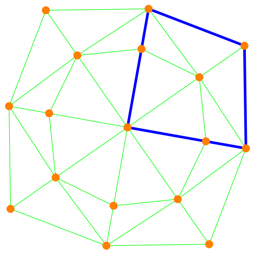
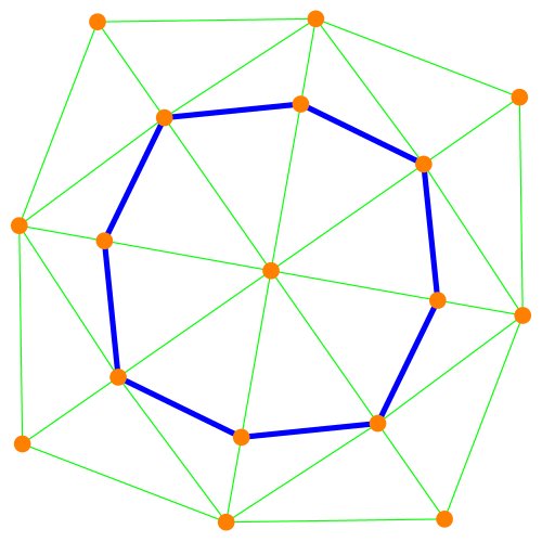
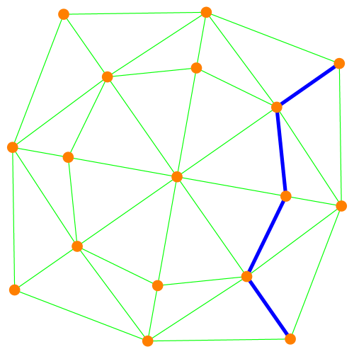
Figure 1. The background complex $G$ is a Barycentric refinement of the wheel graph. The $k=2$ cohomology has the Betti vector $b(G)=(0,0,1,0,0)$. To the very left and very right we see unit sphere subgraphs $H$ which touch the boundary. The Betti vector for the cohomology $H(G,H)$ is $b(G,H)=(0,0,1,0)$ which matches with $\omega(G,H)=1$. In the middle we see a circular subgraph $H$ which does not hit the boundary. In that case the cohomology is $b(G,H)=(0,0,1,1)$ leading to the Wu intersection number $\omega(G,H)=0$.

4.6.

We can have seen examples, where $H$ was a subcomplex of $G$. It is also possible that $G,H$ just intersect. In that case, only a neighborhood of the intersection set matters. We have computed Wu characteristic of nicely intersecting one dimensional graphs. To analyze this, we only need to understand a single intersection cross, where the cohomology is $b(G,H)=(0,0,1)$. Now, if $G$ is a circle and $H$ is a circle and the two circles intersect nicely, we have $b(G,H)=(0,0,2)$ as there are two intersection points.

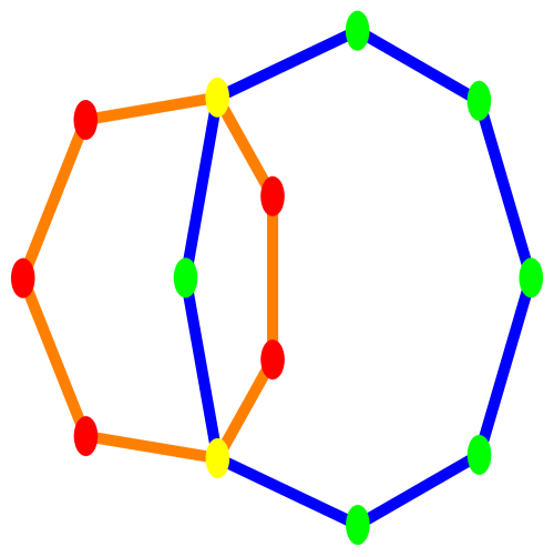
Figure 2. The intersection of two circles $G,H$ has the Betti vector $b(G,H)=(0,0,2)$ and $\omega(G,H)=2$.

5. Hodge relations

5.1.

The Euler-Poincaré relations equating combinatorial and cohomological expressions for $H_{k}^{p}(G)$ can be proven dynamically using the heat flow $\exp(-tL)$. To do so, it is important to build a basis of the cohomology using harmonic forms. For $t=0$, we have by definition the Euler characteristic and for $t\to\infty$, the super trace of the identity on harmonic forms. These Hodge relations play there an important role. It is good to revisit them in the more general frame work of interaction cohomology. The proofs are the same than for $k=1$ however.

5.2.

The Hodge theorem states that $H^{p}(G_{1},\dots,G_{k})$ is isomorphic to the space $E_{0}^{p}(G_{1},\dots<G_{k})$ of harmonic $p$-forms.

Lemma 1.

a) $L$ commutes with $d$ and $d^{*}$,
b) $Lf=0$ is equivalent to $df=0$ and $d^{*}f=0$
c) $f=dg$ and $h=d^{*}k$ are orthogonal.
d) ${\rm im}(d)\cup{\rm im}(d^{*})$ span ${\rm im}(L)$.

Proof.

a) follows from from $d^{2}=(d^{*})^{2}=0$ so that $d^{*}L=Ld^{*}=d^{*}dd^{*}$ and $dL=Ld=dd^{*}d$.
b) if $Lf=0$ then $0=\langle f,Lf\rangle=\langle d^{*}f,d^{f}\rangle+\langle df,df\rangle$ shows that both $d^{*}f=0$ and $df=0$. The other direction is clear.
c) $\langle f,h\rangle=\langle dg,d^{*}k\rangle=\langle ddg,k\rangle=\langle g,d^{*}d^{*}k\rangle=0$.
d) Write $g=Lf=d(d^{*}f)+d^{*}(df)$. ∎

This shows that any $p$-form can be written as a sum of an exact, a co-exact and a harmonic $p$-form:

Lemma 2 (Hodge decomposition).

There is an orthogonal decomposition $\Omega={\rm im}(L)+{\rm ker}(L)={\rm im}(d)+{\rm im}(d^{*})+{\rm ker}(L)$. Any $p$-form $g$ can be written as $g=df+d^{*}h+k$, where $k$ is harmonic.

Proof.

The matrix $L:\Omega(G_{1},\dots,G_{k})\to\Omega(G_{1},\dots,G_{k})$ is symmetric so that the image and kernel are perpendicular. By the lemma, the image of $L$ splits into two orthogonal components ${\rm im}(d)$ and ${\rm im}(d^{*})$. ∎

Theorem 2 (Hodge-Weyl).

The dimension of the vector space of harmonic $p$-forms is equal to $b_{p}(G_{1},\dots,G_{k})$. Every cohomology class has a unique harmonic representative.

Proof.

If $Lf=0$, then $df=0$ and so $Lf=d^{*}df=0$. Given a closed $n$-form $g$ then $dg=0$ and the Hodge decomposition shows $g=df+k$ so that $g$ differs from a harmonic form only by $df$ and so that this harmonic form is in the same cohomology class than $f$. ∎

The harmonic $k$-form represent therefore cohomology classes for the cohomologies $H^{p}(G_{1},\dots,G_{k})$.

6. Lefschetz fixed point formula

6.1.

In the case of Euler characteristic Lefschetz number of an automorphism $T$ of a complex $G$ is the super trace of the induced linear map on simplicial cohomology. If $T$ is the identity, then this is the definition of the cohomological Euler characteristic. We want to show here that the Lefschetz fixed point formula relates more generally the Lefschetz number with the fixed simplices of $T$. If $T$ is the identity, then every simplex is fixed and the Lefschetz fixed point formula is the Euler-Poincaré formula. Since we have a cohomology for Wu characteristic, we can look at the super trace of the map induced on the cohomology groups and get so a new Lefschetz number.

6.2.

We also have fixed pairs of simplices $(x,y)$ and an $2$-interaction index

$$i_{T}(x,y)=\omega(x)\omega(y){\rm sign}(T|x){\rm sign}(T|y)\;.$$

Now, the analogue quadratic theorem is that $L_{2}(T)=\sum_{x\sim y\in G,T(x)=x,T(y)=y}i_{x,y}(T)$, where the sum is over all pairs of simplices, where one is fixed by $T$. This is the Lefschetz fixed point formula for Wu characteristic. In the case of the identity, every pair of intersecting simplices is a fixed point and the Lefschetz fixed point formula reduces to the Euler-Poincarf́ormula for Wu characteristic. For example, for an orientation reversing involution on the circular graph $G=C_{n}$ with $n\geq 4$. The space $H^{0,1}(G)$ is 6-dimensional as is $H^{1,1}(G)$.

6.3.

An automorphism $T$ of $G$ is a permutation on the finite set $V$ of zero-dimensional elements in $G$ such that $T$ induces a permutation on $G$. More generally, one could look also at endomorphisms, maps which map simplices to simplices and preserve the order, but since we are in a finite frame work, we can always restrict to the attractor $\bigcap_{n}T^{n}(G)$ on which $T$ then induces an automorphism. It is therefore almost no restriction of generality to look at automorphisms.

6.4.

Let ${\rm Aut}(G)$ be the group of automorphisms of $G$. Any $T\in Aut(G)$ induces a linear map on each interaction cohomology group $H^{p}_{k}(G)$. To realize that the matrix belonging to the transformation take an orthonormal basis for the kernel of $L_{k}$ and define $A_{ij}=f_{i}(T)f_{j}$. If $L|H(G)$ denotes the induced map on cohomology, define the Lefschetz number $\chi_{T}(G)={\rm str}(L|H(G))$. In the special case, when $T$ is the identity $T=1$, the Lefschetz number is the Wu characteristic. In the case $k=2$, a pair of intersecting simplices $(x,y)$ is called a fixed point of $T$, if $T(x)=x,T(y)=y$. More generally, we call a $k$-tuple $(x_{1},\dots,x_{k})$ of pairwise intersecting simplices to be a fixed point of $T$ if $T(x_{j})=x_{j}$. Define the index of a fixed point as

$$i_{T}(x_{1},\dots,x_{k})=\prod_{j=1}^{k}(-1)^{\rm dim(x_{j})}{\rm sign}(T|x_{j})\;.$$

6.5.

In the case $k=1$, the index is

$$i_{T}(x)=(-1)^{{\rm dim}(x)}{\rm sign}(T|x)\;.$$

In the case $k=2$, the index is

$$i_{T}(x,y)=(-1)^{{\rm dim}(x)+{\rm dim}(y)}{\rm sign}(T|x){\rm sign}(T|y)\;.$$

Here is the Brouwer-Lefschetz-Hopf fixed point formula generalizing [10].

Theorem 3 (Brouwer-Lefschetz fixed point theorem).

$\chi_{T}(G)=\sum_{T(x=x}i_{T}(x)$

The heat proof works as before. For $t=0$ we get the right hand side, for $t\to\infty$ we get the left hand side.

Proof.

Combine the unitary transformation $U:f\to f(T)$ with the heat flow $V(t)=\exp(-tL)$ to get the time-dependent operator $W(t)=UV(t)$ on the linear space of discrete differential forms. For $t=0$, the super trace of $W_{t}$ is $\sum_{x\sim y}i_{T}(x,y)$. McKean-Singer shows that the super trace of any positive power $L^{n}$ of $L$ is always zero. This is the super symmetry meaning that the union of the positive eigenvalues on the even dimensional part of the interaction Laplacian L is the same than the union of the positive eigenvalues on the odd dimensional part of L. For $t\to\infty$, the heat flow kills the eigenspace to the positive eigenvalues and pushes the operator $W(t)$ towards a projection onto the kernel. The projection operator $P$ onto harmonic interaction differential forms is the attractor. Since by Hodge theory the kernel of the Laplacian L¡sub¿m¡/sub¿ on $m$-interaction forms parametrized representatives of the m-th cohomology group, the transformation W(infinity) is nothing else than the induced linear transformation on cohomology. Its super trace is by definition the Lefschetz number. The super symmetry relation ${\rm str}(L^{n})$ for $n>0$ assures that the super trace of $\exp(-tL)$ does not depend on t. The heat flow (mentioned for example in [24]) washes away the positive spectrum and leaves only the bare harmonic part responsible for the cohomology description. For $T=1$, the heat flow interpolates between the combinatorial definition of the Wu characteristic and the cohomological definition of the Wu characteristic, similarly as in the case of the Euler characteristic. ∎

6.6.

Also, as in the case $k=1$, we can average the Lefschetz number over a subgroup $A$ of the automorphism group of $G$ to get $\omega_{k}(G/A)$, where $G/A$ is the quotient chain. If we look at the Barycentric refinement, we can achieve that the quotient chain is again a simplicial complex. These are generalizations of Riemann-Hurwitz type results.

7. Barycentric invariance

7.1.

Almost by definition, the Wu characteristic $\omega(G)$ is multiplicative

$$\omega(G\times H)=\omega(G)\omega(H)\;$$

because

$$\sum_{(x,y)\sim(u,v)}\omega(x)\omega(y)\omega(u)\omega(v)=(\sum_{x\sim u}\omega(x)\omega(u))(\sum_{y\sim v}\omega(y)\omega(v))\;.$$

The same product formula holds for the other cases $\omega_{k}(G\times H)=\omega_{K}(G)\omega_{K}(H)$. This relation has used the Cartesian product $G\times H$ of simplicial complexes which is not a simplicial complex any more. In [19] we have looked at the product $(G\times H)_{1}$, the Barycentric refinement of $G\times H$ so that we would remain in the class of simplicial complexes. But because calculus can be done equally well on the ring itself, there is no need any more to insist on having simplicial complexes. Indeed, in the strong ring, the simplicial complexes are the multiplicative primes.

Proposition 1.

All the Wu characteristics $\omega_{k}$ are ring homomorphisms from the strong ring to the integers.

Proof.

The additivity $\omega_{k}(G+H)=\omega_{k}(G+H)$ for the disjoint union is clear as all $\omega_{k}$ are multi-linear valuations and $\omega_{k}(0)=0$. The compatibility with multiplication follows from $\omega_{k}(1)=1$ for all $k$ and

$$\omega_{k}(G\times H)=\sum_{(x_{1},\dots,x_{k})\sim(y_{1},\dots,y_{k})}\omega(x_{1})\cdots\omega(x_{k})\omega(y_{1})\cdots\omega(y_{k})$$

$$(\sum_{(x_{1},\dots,x_{k})}\omega(x_{1})\cdots\omega(x_{k}))(\sum_{(y_{1},\dots,y_{k})}\omega(y_{1})\cdots\omega(y_{k}))$$

$$=\omega_{k}(G)\omega_{k}(H)$$

∎

7.2.

Given a simplicial complex $G$ defined over a set $V$ of “vertices”, zero dimensional sets in $G$, the complex $G_{1}$ is defined over the set $V_{1}=G$. We call a vertex $x$ in $G_{1}$ a $p$-vertex, if it had been a $p$-dimensional simplex in $G$.

Theorem 4 (Barycentric Invariance).

$H^{p}_{k}(G)=H^{p}_{k}(G_{1})$.

Proof.

There is an explicit map $\phi$ from the space of forms on $G$ to the space of forms in $G_{1}$. Lets look at it first in the case $k=1$.
Given a $p$-simplex $(x_{1},\dots,x_{p})$ in $G_{1}$, there is maximally one of the vertices where $F$ is non-zero. Define $F(x_{1},\dots,x_{p})=F(x_{k})/p!$ to be this value. On the other hand, given a form $F$ on $G_{1}$, we get a form on $G$. Given a simplex $x$ in $G$ it contains $p!$ simplices of the same dimension in $G_{1}$. Now just sum up the $F$ values over these simplices. As $\phi$ and its inverse commute with the exterior derivative $d$ in the sense $d(G_{1})\phi=\phi d(G)$, we have also $L(G_{1})\phi=\phi L(G)$. Harmonic forms are mapped into Harmonic forms.
More generally, the Barycentric invariance works for $H^{p}(G_{1},\dots,G_{k})$, which is isomorphic to $H^{p}((G_{1})_{1},\dots,(G_{k})_{1})$, where $(G_{j})_{1}$ is the Barycentric refinement of $G_{j}$. The map $\phi$ from forms in $\Omega(G_{1},\dots,G_{k})$ to forms in $\Omega((G_{1})_{1},\dots,(G_{k})_{1})$ just distributes the value $F(x_{1},\dots,x_{k})$ on pairwise intersecting simplices $x_{1},\dots,x_{k}$ equally to all $k$-tuples of pairwise intersecting simplices $y_{1},\dots,y_{k})$ with $y_{j}$ being simplices of the same dimension than $x_{j}$ within $x_{j}$. The inverse of $\phi$ sums all values up. These averaging procedures commute with $d$. ∎

7.3.

We don’t know yet whether there is a more robust statement. We would think for example that if $H_{1},H_{2}$ are two complexes, where one is a Barycentric refinement of the other and both are embedded in the same way in a larger graph $G$, then $H^{p}(G,H_{1})=H^{p}(G,H_{2})$. Experiments indicated that this is true. We also have hopes that if $H_{1},H_{2}$ are two different knots embedded into a three dimensional discrete sphere $G$, then we could distinguish the embedding by computing $H^{p}(G,H_{1})$ and $H^{p}(G,H_{2})$. We also need to look at the cohomology of the complement $H^{p}(G,G\setminus H_{1})$ and $H^{p}(G,G\setminus H_{2})$. Classically, one has used simplicial cohomology $H^{p}(G\setminus H_{1}),H^{p}(G\setminus H_{2})$ already.

8. Kuenneth formula

8.1.

The Barycentric refinement invariance shows that that the cohomology of $(G\times H)_{1}$ is the same than the cohomology of $G\times H$. So, we could for $k=1$ refer to [19] to get

Theorem 5 (Kuenneth).

$H_{k}^{p}(G\times H)=\oplus_{i+j=p}H_{k}^{i}(G)\oplus H_{k}^{j}(H)$.

8.2.

The proof follows from Hodge and the proposition stated below. Instead of generalizing [19] from $k=1$ to larger $k$, it is better to prove the relation directly first for the Cartesian product (which is not a simplicial complex), and then invoke the Barycentric refinement, to recover [19]. Now this is just Hodge. We have to show that for every $k$, every harmonic $p$-form $f$ can be written as a pair $(g,h)$, where $g$ is an $i$-form and $h$ is a $j$ form.

8.3.

Künneth could not be more direct:

Proposition 2.

A basis for $H^{p}(G,H)$ is given by $L$-harmonic $p$-forms $v$. A basis for $L(G,H)$-Harmonic $p$-forms is given by all the vectors $v\oplus w$, where $v$ is $L(G)$-harmonic $k$-form and $w$ is $L(H)$-harmonic $m$-form so that $k+m=p$.

8.4.

In [19] the construction of a chain homotopy was more convoluted as we dealt with the Barycentric refinements (as at time, we felt we needed to work with simplicial complexes). Separating the two things and establishing the Barycentric invariance separately is more elegant.

8.5.

For a given $k$ and ring element $G$, define the Poincaré polynomial

$$p_{G,k}(t)=\sum_{l=0}b_{k,l}(G)t^{l}\;.$$

If $k=1$, then $p_{G}(t)=p_{G,1}(t)$ is the usual Poincaré polynomial.

Corollary 1.

The map $G\to p_{G,k}(t)$ is a ring homomorphism from the strong connection ring to $\mathbb{Z}[t]$.

Proof.

If $d_{i}$ are the exterior derivatives on $G_{i}$, we can write them as partial exterior derivatives on the product space. We get from $df(x,y)=d_{1}f(x,y)+(-1)^{{\rm dim}(x)}d_{2}(f(x,y)$

$$d^{*}df=d_{1}^{*}d_{1}f+(-1)^{{\rm dim}(x)}d_{1}^{*}d_{2}f+(-1)^{{\rm dim}}d_{2}^{*}d_{1}f+d_{2}^{*}d_{2}f\;,$$

$$dd^{*}f=d_{1}d_{1}^{*}f+(-1)^{{\rm dim}(x)}d_{1}d_{2}^{*}f+(-1)^{{\rm dim}(x)}d_{2}d_{1}^{*}f+d_{2}d_{2}^{*}f\;.$$

Therefore $Hf=H_{1}f+H_{2}f+(-1)^{{\rm dim}(x)}(d_{1}^{*}d_{2}+d_{1}d_{2}^{*}+d_{2}^{*}d_{1}+d_{2}d_{1}^{*})f(x,y))$. Since Hodge gives an orthogonal decomposition

$${\rm im}(d_{i}),{\rm im}(d_{i}^{*}),{\rm ker}(H_{i})={\rm ker}(d_{i})\cap{\rm ker}(d_{i}^{*})\;,$$

there is a basis in which $H(v,w)=(H(G_{1})(v),H(G_{2})(w))$. Every kernel element can be written as $(v,w)$, where $v$ is in the kernel of $H_{1}$ and $w$ is in the kernel of $H_{2}$. ∎

8.6.

In the special case $k=1$, the Kuenneth formula would follow also from [19] because the product is $(G\times H)_{1}$ and the cohomology of the Barycentric refinement is the same. It follows that the Euler-Poincaré formula holds in general for elements $G$ in the ring: the cohomological Euler characteristic $\sum_{k=0}^{\infty}b_{k}(G)(-1)^{k}$ is equal to the combinatorial Euler characteristic $\sum_{k=0}^{\infty}v_{k}(G)(-1)^{k}$, where $(v_{0},v_{1},\dots)$ is the $f$-vector of $G$. Note that the Cartesian product $G\times H$ of two signed simplicial complexes is still a signed discrete CW complex so that one can define $v_{k}(G\times H)$ as the number of $k$-dimensional cells in $G\times H$.

9. Euler polynomial

9.1.

Every ring element $G$ in the strong ring has a $f$-vector $(v_{0},v_{1},v_{2},\dots,v_{r})$. Unlike for a simplicial complex, the entries are now general integers and not non-negative integers. This defines the Euler polynomial

$$e_{G}(t)=\sum_{l=0}v_{l}(G)t^{l}\;.$$

The Euler-Poincaré relations can be stated as $e_{G}(-1)=p_{G}(-1)$. This is a relation which holds for any ring element.

9.2.

The Poincaré polynomial relates with the Euler polynomial, which also has a nice algebraic description:

Proposition 3 (Euler polynomial).

The map $G\to e_{G}(t)$ is a ring homomorphism from the strong connection ring to $\mathbb{Z}[t]$.

Proof.

When doing a disjoint union, the cardinalities add. For the Cartesian product, we take the set theoretical Cartesian product $G\times H$ of sets of sets. Now, if $x$ has dimension $p$ and $y$ has dimension $q$, then $x\times y$ has dimension $p+q$. ∎

9.3.

There are higher dimensional versions of the Euler polynomial. Let $V=V_{k,l}$ denote the $f$-vector of $G$, where $V_{k,l}$ are the number of pairs $(x,y)$ of simplices which intersect and ${\rm dim}(x)=k$ and ${\rm dim}(y)=l$. We can now define multi-variate Euler polynomials like the quadratic Euler polynomial

$$e_{G,2}(s,t)=\sum_{i,j}V_{i,j}s^{i}t^{j}\;,$$

which is a generating function for the $f$-matrix. The definition of the Wu characteristic gives $\omega_{2}(G)=e_{G,2}(-1,-1)$.

9.4.

Examples.
1) For $G=K_{2}$, we have $e_{G}(t)=2+t$ and $e_{G,2}(t,s)=2+2t+2s+ts$ which leads to $\chi(G)=e_{G}(-1)=1$ and $\omega(G)=e_{G,2}(-1,-1)=-1$.
2) For $G=K_{3}$, we have $e_{G}(t)=3+3t+t^{2}$ and $e_{G,2}(t,s)=s^{2}t^{2}+3s^{2}t+3s^{2}+3st^{2}+9st+6s+3t^{2}+6t+3$ leading to $\omega(G)=e_{G,3}(-1,-1)=1$.

9.5.

Similarly, one can define $f$-tensors for any $k$. They encode the cardinalities of interacting $k$-tuples of simplices. The multivariate Euler polynomial is then

$$e_{G,k}(t_{1},\dots,t_{k})=\sum_{j_{1},j_{2},\dots,j_{k}}V_{j_{1},\dots,j_{k}}t_{1}^{j_{1}}\cdots t_{k}^{j_{k}}\;.$$

For example, for $G=K_{2}$, we have $e_{G}(t_{1},t_{2},t_{3})=2+2t_{1}+2t_{2}+2t_{3}+2t_{1}t_{2}+2t_{1}t_{3}+2t_{2}t_{3}+t_{1}t_{2}t_{3}$ which gives $\omega_{3}(G)=e_{G}(-1,-1,-1)=1$.

Proposition 4 (Euler polynomial).

The map $G\to e_{G,k}(t_{1},\dots,t_{k})$ is a ring homomorphism from the strong ring to $\mathbb{Z}[t_{1},\dots,t_{k}]$.

Proof.

Again, the additive part is clear. For the multiplication, if $(x_{1}\times\cdots x_{k})$ intersects $(y_{1}\times\cdots y_{k})$, this happens if each $x_{j}$ intersects each $y_{j}$. The intersection of simplices $x_{1},x_{2},\dots x_{k}$ of dimension $r_{1},\dots,r_{k}$ is represented algebraically by $t_{1}^{r_{1}}t_{2}^{r_{2}}\cdots t_{k}^{r_{k}}$. The intersection of simplices $y_{1},y_{2},\dots y_{k}$ of dimension $s_{1},\dots,s_{k}$ is represented algebraically by $t_{1}^{s_{1}}t_{2}^{s_{2}}\cdots t_{k}^{s_{k}}$. If we take the product, we get $t_{1}^{r_{1}+s_{1}}t_{2}^{r_{2}+s_{2}}\cdots t_{k}^{r_{k}+s_{k}}$ which represents the intersection of simplices $(x_{1}\times y_{1}),(x_{2}\times y_{2}),\dots(x_{k}\times y_{k})$ of dimension $r_{1}+s_{1},\dots,r_{k}+s_{k}$. ∎

9.6.

Having a multivariate ring homomorphism for the Euler polynomial suggests going back to the cohomology and redefining the cohomology so that the Poincaré polynomial becomes a multivariate polynomial too. This is indeed possible because the exterior derivative $d=d_{1}+\cdots+d_{k}$ is a sum of partial exterior derivatives which each satisfy $d_{j}^{2}=0$. So, we get a cohomology Betti tensor $b$ which is in the case $k=2$ a cohomology Betti matrix. One could define htne a multivariate Poincaré polynomial $p_{G,k}(t_{1},\dots,t_{k})$ and the map $G\to p_{G,k}(t_{1},\dots,t_{k})$ is a ring homomorphism from the strong ring to $\mathbb{Z}[t_{1},\dots,t_{k}]$. One can get the Poincaré polynomial (as we have defined it) by setting $p_{G,k}(t,t,\dots,t)$. This is how we have initially defined the cohomology (see the appendix). Euler-Poincare $p_{G,k}(-1,-1,\dots,-1)=e_{G,k}(-1,-1,\dots,-1)$ still holds, but there is a problem: the Betti matrix is not invariant under Barycentric refinements, similarly as the $f$-matrix is not invariant under Barycentric refinement. A sensible cohomology should be invariant under Barycentric refinement.

10. Miscellaneous

10.1.

Any exterior derivative can be deformed via a Lax deformation [13, 12]. There is a version which keeps the exterior derivative $d$ real

$$\dot{D}=[B(D),D],B(t)=d(t)-d^{*}(t),D(t)=d(t)+d(t)^{*}+b(t)\;.$$

Then there is a version which allows the operators to become complex:

$$\dot{D}=[B(D),D],B(t)=d(t)-d^{*}(t)-ib(t),D(t)=d(t)+d(t)^{*}+b(t)\;.$$

This works in the same way also for the exterior derivative $d$ of interaction cohomology. In the first case, we have a scattering situation, in the second we get asymptotically to a linear wave equation.

10.2.

Having deformations in the division algebras $\mathbb{R}$ and $\mathbb{C}$, one can ask whether it is also possible in the third and last associative division algebra, the quaternions $\mathbb{H}$. Given a real exterior derivative we can form $D=d+d^{*}$ and deform it with $D^{\prime}=[B,D]$, where $B=d-d^{*}+I(b+b^{*})$, where $I=oi+pj+qk$ is a space quaternion. Given by three real commuting complexes $D_{1},D_{2},D_{3}$, we can start with the initial condition $D=iD_{1}+jD_{2}+kD_{3}$. We initially have the Pythagorean relation $L=D^{2}=-L_{1}^{2}-L_{2}^{2}-L_{3}^{2}$. Quaternions are best implemented as complex $2\times 2$ matrices using Pauli matrices $\sigma_{i}$. The real number $1$ is represented by the identity matrix, the standard imaginary square root of $-1$ is $i\sigma_{3}$, the quaternion $j$ is $i\sigma_{2}$ and the quaternion $k$ is $i\sigma_{1}$. In other words, the explicit translation from a quaternion $a+ib+jc+kd$ to a complex $2\times 2$ matrix $\left[\begin{array}[]{cc}a+ib&c+id\\ -c+id&a-ib\end{array}\right]$. The complex parameter $I$ is now just an arbitrary element in the Lie algebra of $SU(2)$.

10.3.

Example. Take the smallest simplicial complex $G=\{\{1\},\{2\},\{1,2\}\}$ for which $D=\left[\begin{array}[]{ccc}0&0&-1\\ 0&0&1\\ -1&1&0\\ \end{array}\right]$. To evolve in the quaternion domain, take three copies and glue them together to get the new quaternion valued Dirac operator:

$$D=\left[\begin{array}[]{cccccc}0&0&0&0&-i&-1-i\\ 0&0&0&0&1-i&i\\ 0&0&0&0&i&1+i\\ 0&0&0&0&-1+i&-i\\ -i&-1-i&i&1+i&0&0\\ 1-i&i&-1+i&-i&0&0\\ \end{array}\right]\;.$$

Its Laplacian $L=D^{2}$ is just the original Hodge Laplacian, where each entry $1$ is replaced with a $2\times 2$ identity matrix. Here is the deformed operator at time $t=0.1$ in the case $I=i$ (the quaternion $i$):

$$D(t)=\left[\begin{array}[]{cccccc}0\,+0.36i&0.38\,+0.33i&0\,-0.36i&-0.38-0.33i&-0.19-0.85i&-0.86-0.86i\\ -0.38+0.33i&0\,-0.36i&0.38\,-0.33i&0\,+0.36i&0.86\,-0.86i&-0.19+0.85i\\ 0\,-0.36i&-0.38-0.33i&0\,+0.36i&0.3\,+0.33i&0.19\,+0.85i&0.86\,+0.86i\\ 0.38\,-0.33i&0\,+0.36i&-0.38+0.33i&0\,-0.36i&-0.86+0.86i&0.19\,-0.85i\\ 0.19\,-0.85i&-0.86-0.86i&-0.19+0.85i&0.86\,+0.86i&0\,-0.72i&-0.67-0.77i\\ 0.86\,-0.86i&0.19\,+0.85i&-0.86+0.86i&-0.19-0.85i&0.67\,-0.77i&0\,+0.72i\\ \end{array}\right]\;.$$

10.4.

Let $G$ be a finite abstract simplicial complex with Barycentric refinement $G_{1}$ and let $n$ be the number of simplices of $G$. The connection graph $G^{\prime}$ of $G$ is defined as the graph with vertex set $G$, and where two vertices are connected, if they intersect. The graph $G_{1}$ is a subgraph of $G^{\prime}$. Already the case of a cyclic graph shows that $G^{\prime}$ has in general a higher dimension than $G$. Define the connection matrix $L$ by $L(x,y)=1$ if $x\cap y\neq\emptyset$ and $L(x,y)=0$ else.

10.5.

The diagonal entries of $L$ correspond to self interactions, the side diagonal elements are interactions between simplices. With $S={\rm Diag}((-1)^{{\rm dim}(x)})$, define $J=S^{-1}IS$, where $I$ is the matrix containing only $1$. The matrix satisfies $J_{ij}=(-1)^{i+j}$. It is a checkerboard matrix. Define the Wu matrix $WJ$. We are interested in the matrix $W$ because it gives the Wu characteristic: the Wu characteristic $\omega(G)$ of a finite simple graph is equal to ${\rm tr}(WJ)$.

10.6.

A square matrix is called unimodular if its determinant is either $-1$ or $1$. This implies that all entries of the inverse are integer-valued. While the Fredholm determinant of a general graph can be pretty arbitrary, the Fredholm determinant of a connection graph is always plus or minus $1$ implying that $L^{-1}$ is always an integer matrix. Define the Fredholm characteristic $\psi(G)={\rm det}(L)$ and the Fermi characteristic $\phi(G)=\prod_{x}\omega(x)$, where the sum is over all simplices in $G$ and $\omega(x)=(-1)^{{\rm dim}(x)}$.

10.7.

For any finite simple graph, the Fredholm matrix $L$ of its connection matrix is unimodular: $\psi(G)=\phi(G)$. (We were writing this paragraph of the current paper, when the unimodularity discovery happend, delaying this by 2 years).

10.8.

Finally, we notice that the graph $G_{1}^{\prime}$ and $G_{1}$ are homotopic. It is not true without a refinement step. The octahedron graph $G$ has a connection graph $G^{\prime}$ which is not homotopic to $G$: the Euler characteristic of the connection graph is $0$. Its $f$-vector is $(26,180,556,918,900,560,224,54,6)$. Its Betti vector is $(1,0,0,1,0,0,0,0,0)$. It is topologically a 3-sphere, a Hopf fibration of the 2-sphere as the graph has developed a nontrivial three dimensional cohomology. It is not contractible. If one removes all zero dimensional vertices, we still have the same cohomology but a smaller graph with f-vector $v(G)=(20,132,388,582,480,224,56,6)$.

10.9.

The Fredholm determinant of a Barycentric refinement $G_{1}$ of a graph $G$ is always $1$. There is an explicit linear map $f(G)\to Af=f(G_{1})$ which gives the $f$-vector of the Barycentric refinement $G_{1}$ from $G$. The image always has an even number of odd-dimensional simplices.

10.10.

There are various other connection matrices or connection tensors one could look at. For any $k$ one can look at the tensor $L(x_{1},\dots,x_{k})$ which is $1$ if the simplices $x_{1},\dots,x_{k}$ pairwise intersect and $0$ else. But it is the quadratic case which obviously is the most important one as we then have a matrix which has a determinant and eigenvalues. An other structure we have looked at but not found useful yet is to look at the set of intersecting simplices $(x,y)$. If there are $n$ such pairs, look at the $n\times n$ matrix which is $L((x,y),(u,v))=1$ if $(x,y)$ and $(u,v)$ intersect somewhere and $0$ else. One can similarly define such intersection matrices for $k>2$ also. So far, we have not yet discovered a nice algebraic fact like the unimodularity of the connection matrix.

10.11.

In any case, whatever Laplacian is taken, we can look at it in the Barycentric limit [18, 20].

11. Historical remarks

11.1. About simplicial complexes

11.2.

Abstract simplicial complexes were first defined in 1907 by Dehn and Heegaard [3] and used further by Tietze, Brouwer, Steinitz, Veblen, Whitney, Weyl and Kneser. In [1], Alexandroff calls a simplicial complex an unrestricted skeleton complex, whereas any finite sets is a skeleton complex. Still mostly used in Euclidean settings like [7], modern topology textbooks like [33, 32] or [31] use the abstract version. A generalization of simplicial complexes are simplicial sets.

11.3.

In [32], the join of two simplicial complexes is defined. The definition for graphs goes back to Zykov [36]. In [8, 34], the empty set, the ”void” is included in a complex. This leads to reduced $f$-vectors $(v_{-1},v_{0},...)$ with $v_{-1}=1$ and reduced Euler characteristic $\chi(G)-1$ known in enumerative combinatorics. The number $1-\chi(G)$ is in one-dimensions the genus. It is multiplicative when taking joins of simplicial complexes.

11.4. About Wu characteristic

Wu defines the characteristic numbers through the property that none of the simplices intersect. Lets call this $\tilde{\omega}(G)$. For $k=2$, one can write this as $\chi(G)^{2}-\tilde{\omega}(G)$ so that we have nothing new when defining this. For the higher order versions however, the relations are no more so direct. We should also note that Wu, as custom for combinatorial topology in the 20’th century, dealt with polytopes. But since there are various definitions of polytopes [6], we don’t use that language.

12. Questions

12.1.

Since we do not have homotopy invariance but invariance under Barycentric refinement, an important question is whether the cohomology is a topological invariant in the sense of [17]. Under which conditions is it true that if $H_{1},H_{2}$ are homeomorphic and $G\setminus H_{1}$ and $G\setminus H_{2}$ are topologically equivalent, then then $H^{p}(G,H_{1})=H^{p}(G,H_{2})$? Is it true that $H^{p}(H_{1})=H^{p}(H_{2})$? We believe that both statements are true. The intuition comes from the believe that there is a continuum limit, where we can do deformations. One attempt to construct a continuum cohomology is to look at the product complex of the usual de-Rham complex on the product $M\times M$ of a manifold $M$, then take a limit of equivalence relations where a pair $(f,g)$ of $k$ and $l$ forms with $k+l=p$ is restricted to the diagonal. If the Hodge story goes over, then the homotopy invariance follows from elliptic regularity assuring that there is a positive distance between the zero eigenvalues and the next larger eigenvalue. A small deformation of the geometry changes the eigenvalues continuously so that the kernel of the Hodge operators on $p$-forms stay robust. This strategy could work while staying within the discrete: when doing Barycentric refinements, we can make the spectral effect of a homotopy deformation small.

12.2.

Also not explored is what the Betti numbers of a $d$-complex with or without boundary are. We have already a boundary formula $\omega_{2}(G)=\omega(G)=\chi(G)-\chi(\delta{G})$ for Wu characteristic. Are there formulas for the Betti numbers in that case which relate the simplicial Betti numbers of $G$ and $\delta G$ with the Betti numbers of the $k=2$ cohomology.

12.3.

We have seen that for the quadratic cohomology, there are examples of complexes like the Möbius strip which have trivial cohomology in the sense that the Betti vector is 0. This is equivalent to the fact that the Hodge Laplacian is invertible. This obviously does not happen for simplicial cohomology but the Möbius strip is an example for interaction cohomology. One can ask which spaces have this property. Such a space necessarily has to have zero Wu characteristic.

12.4.

We have tried to compute the cohomology of the Poincaré Homology sphere which is generated by $\{\{1,2,4,9\}$, $\{1,2,4,15\}$, $\{1,2,6,14\}$, $\{1,2,6,15\}$, $\{1,2,9,14\}$, $\{1,3,4,12\}$, $\{1,3,4,15\}$, $\{1,3,7,10\}$, $\{1,3,7,12\}$, $\{1,3,10,15\},\{1,4,9,12\}$, $\{1,5,6,13\}$, $\{1,5,6,14\}$, $\{1,5,8,11\}$, $\{1,5,8,13\}$, $\{1,5,11,14\}$, $\{1,6,13,15\}$, $\{1,7,8,10\}$, $\{1,7,8,11\}$, $\{1,7,11,12\},\{1,8,10,13\}$, $\{1,9,11,12\}$, $\{1,9,11,14\}$, $\{1,10,13,15\}$, $\{2,3,5,10\}$, $\{2,3,5,11\}$, $\{2,3,7,10\}$, $\{2,3,7,13\}$, $\{2,3,11,13\}$, $\{2,4,9,13\},\{2,4,11,13\}$, $\{2,4,11,15\}$, $\{2,5,8,11\}$, $\{2,5,8,12\}$, $\{2,5,10,12\}$, $\{2,6,10,12\}$, $\{2,6,10,14\}$, $\{2,6,12,15\}$, $\{2,7,9,13\}$, $\{2,7,9,14\},\{2,7,10,14\}$, $\{2,8,11,15\}$, $\{2,8,12,15\}$, $\{3,4,5,14\}$, $\{3,4,5,15\}$, $\{3,4,12,14\}$, $\{3,5,10,15\}$, $\{3,5,11,14\}$, $\{3,7,12,13\},\{3,11,13,14\}$, $\{3,12,13,14\}$, $\{4,5,6,7\}$, $\{4,5,6,14\}$, $\{4,5,7,15\}$, $\{4,6,7,11\}$, $\{4,6,10,11\}$, $\{4,6,10,14\}$, $\{4,7,11,15\}$, $\{4,8,9,12\},\{4,8,9,13\}$, $\{4,8,10,13\}$, $\{4,8,10,14\}$, $\{4,8,12,14\}$, $\{4,10,11,13\}$, $\{5,6,7,13\}$, $\{5,7,9,13\}$, $\{5,7,9,15\}$, $\{5,8,9,12\}$, $\{5,8,9,13\},\{5,9,10,12\}$, $\{5,9,10,15\}$, $\{6,7,11,12\}$, $\{6,7,12,13\}$, $\{6,10,11,12\}$, $\{6,12,13,15\}$, $\{7,8,10,14\}$, $\{7,8,11,15\}$, $\{7,8,14,15\},\{7,9,14,15\}$, $\{8,12,14,15\}$, $\{9,10,11,12\}$, $\{9,10,11,16\}$, $\{9,10,15,16\}$, $\{9,11,14,16\}$, $\{9,14,15,16\}$, $\{10,11,13,16\}$, $\{10,13,15,16\},\{11,13,14,16\}$, $\{12,13,14,15\}$, $\{13,14,15,16\}\}$. The corresponding Laplacian is a $70616\times 70616$ matrix. Unfortunately, our computing resources were not able yet to find the kernel of its blocks yet. It would be nice to compare the interaction cohomology of the homology sphere with the interaction cohomology of the 3-sphere.

Appendix: Code

The Mathematica procedure ”Coho2” computes in less than 12 lines a basis for all the cohomology groups $H^{p}(G,H)$ for a pair of simplicial complexes $G,H$. We display then the Betti numbers $b_{p}(G,H)={\rm dim}(H^{p}(G,H))$. As in the text, the case $H^{p}_{2}(G)$ is the same than $H^{p}(G,G)$.

⬇

Coho2[G_,H_]:=Module[{},n=Length[G];m=Length[H];len[x_]:=Total[Map[Length,x]];U={};

Do[If[Length[Intersection[G[[i]],H[[j]]]]>0,U=Append[U,{G[[i]],H[[j]]}]],{i,n},{j,m}];

U=Sort[U,len[#1]<len[#2] & ];u=Length[U];l=Map[len,U]; w=Union[l];

b=Prepend[Table[Max[Flatten[Position[l,w[[k]]]]],{k,Length[w]}],0]; h=Length[b]-1;

deriv1[{x_,y_}]:=Table[{Sort[Delete[x,k]],y},{k,Length[x]}];

deriv2[{x_,y_}]:=Table[{x,Sort[Delete[y,k]]},{k,Length[y]}];

d1=Table[0,{u},{u}]; Do[v=deriv1[U[[m]]]; If[Length[v]>0,

Do[r=Position[U,v[[k]]]; If[r!={},d1[[m,r[[1,1]]]]=(-1)^k],{k,Length[v]}]],{m,u}];

d2=Table[0,{u},{u}]; Do[v=deriv2[U[[m]]]; If[Length[v]>0,

Do[r=Position[U,v[[k]]]; If[r!={},d2[[m,r[[1,1]]]]=(-1)^(Length[U[[m,1]]]+k)],

{k,Length[v]}]],{m,u}]; d=d1+d2; Dirac=d+Transpose[d]; L=Dirac.Dirac; Map[NullSpace,

Table[Table[L[[b[[k]]+i,b[[k]]+j]],{i,b[[k+1]]-b[[k]]},{j,b[[k+1]]-b[[k]]}],{k,h}]]];

Betti2[G_,H_]:=Map[Length,Coho2[G,H]];Coho2[G_]:=Coho2[G,G]; Betti2[G_]:=Betti2[G,G];

Generate[A_]:=Sort[Delete[Union[Sort[Flatten[Map[Subsets,A],1]]],1]];

moebius=Generate[{{1,2,5},{1,4,5},{1,4,7},{2,3,6},{2,5,6},{3,6,7},{4,3,7}}];

Print[”Moebius␣Strip:␣”,Betti2[moebius]];

cylinder=Generate[{{1,2,5},{1,4,8},{1,5,8},{2,3,6},{2,5,6},{3,4,7},{3,6,7},{4,7,8}}];

Print[”Cylinder:␣”,Betti2[cylinder]];

circle=Generate[{{1,2},{2,3},{3,4},{4,5},{5,1}}];

Print[”Circle:␣”,Betti2[circle]];

figureeight=Generate[{{1,2},{1,4},{2,3},{2,5},{2,7},{3,4},{5,6},{6,7}}];

Print[”Figure␣Eight:␣”,Betti2[figureeight]];

point=Generate[{{1}}];

Print[”1-simplex:␣”,Betti2[point]];

segment=Generate[{{1,2}}];

Print[”2-simplex:␣”,Betti2[segment]];

triangle=Generate[{{1,2,3}}];

Print[”3-simplex:␣”,Betti2[triangle]];

tetrahedron=Generate[{{1,2,3,4}}];

Print[”4-simplex:␣”,Betti2[tetrahedron]];

Print[”Point␣in␣interval:␣”,Betti2[{{1,2},{2,3},{1},{2},{3}},{{2}}]];

Print[”Point␣on␣boundary:␣”,Betti2[{{1,2},{2,3},{1},{2},{3}},{{1}}]];

house=Generate[{{1,2},{2,3},{3,4},{4,1},{2,3,5}}];

Print[”House␣graph:␣”,Betti2[house]];

octahedron=Generate[{{1,2,3},{1,2,4},{1,3,5},{1,4,5},{2,3,6},{2,4,6},{3,5,6},{4,5,6}}];

Print[”Octahedron:␣”,Betti2[octahedron]];

equator=Generate[{{2,3},{3,5},{5,4},{4,2}}];

Print[”Circle␣in␣octahedron:␣”,Betti2[octahedron,equator]];

kleinbottle=Generate[{{1,2,3},{1,2,6},{1,3,5},{1,4,7},{1,4,8},{1,5,7},

{1,6,8},{2,3,7},{2,4,6},{2,4,8},{2,5,7},{2,5,8},{3,4,6},{3,4,7},{3,5,6},{5,6,8}}];

Print[”Klein␣bottle:␣”,Betti2[kleinbottle]];

projectiveplane=Generate[{{1,2,5},{1,2,9},{1,4,5},{1,4,7},{1,8,7},{1,8,9},{2,3,6},

{2,3,10},{2,5,6},{2,9,10},{3,6,7},{3,10,11},{4,3,7},{4,3,11},{4,5,12},

{4,11,12},{5,6,13},{5,12,13},{6,7,14},{6,13,14},{8,7,14},{8,9,15},

{8,14,15},{9,10,15},{10,11,15},{11,12,15},{12,13,15},{13,14,15}}];

Print[”Projective␣Plane:␣”,Betti2[projectiveplane]];

Print[”The␣next␣computation␣deals␣with␣4160x4160␣matrices:␣patience␣please␣”];

threesphere=Generate[{{1,3,5,7},{1,3,5,8},{1,3,6,7},{1,3,6,8},

{1,4,5,7},{1,4,5,8},{1,4,6,7},{1,4,6,8},{3,5,7,2},{3,5,8,2},

{3,6,7,2},{3,6,8,2},{4,5,7,2},{4,5,8,2},{4,6,7,2},{4,6,8,2}}];

Print[”3-sphere:␣”,Betti2[threesphere]];

RandomSimplComplex[n_,m_]:=Module[{A={},X=Range[n],k},Do[k:=1+Random[Integer,n-1];

A=Append[A,Union[RandomChoice[X,k]]],{m}];Generate[A]];

Print[”Random␣Complex:␣”,Betti2[RandomSimplComplex[6,10]]]

Appendix: math table talk: ”Wu Characteristic”

This was a Handout to ”Wu Characteristic”, a Harvard math table talk given on March 8, 2016 [30]. It was formulated in the language of graphs. In that talk, the exterior derivative was not yet finalized. It gave a cohomology which was not yet invariant under Barycentric refinements.

Definitions. Let $G=(V,E)$ be a finite simple graph with vertex set $V$ and edge set $E$. The $f$-vector $v(G)=(v_{0}(G),v_{1}(G),\dots,v_{d}(G))$ contains as coordinates the number $v_{k}(G)$ of complete subgraphs $K_{k+1}$ of $G$. These subgraphs are also called k-simplices or cliques. The $f$-matrix $V(G)$ has the entries $V_{ij}(G)$ counting the number of intersecting pairs $(x,y)$, where $x$ is a $i$-simplex and $y$ is a $j$-simplex in $G$. The Euler characteristic of $G$ is $\chi(G)=\sum_{i}(-1)^{i}v_{i}(G)$. The Wu characteristic of $G$ is $\omega(G)=\sum_{ij}(-1)^{i+j}V_{ij}(G)$. If $A,B$ are two graphs, the graph product is a new graph which has as vertex set the set of pairs $(x,y)$, where $x$ is a simplex in $A$ and $y$ is a simplex in $B$. Two such pairs $(x,y),(a,b)$ are connected in the product if either $x\subset a,y\subset b$ or $a\subset x,b\subset y$. The product of $G$ with $K_{1}$ is called the Barycentric refinement $G_{1}$ of $G$. Its vertices are the simplices of $G$. Two simplices are connected in $G_{1}$ if one is contained in the other. If $W$ is a subset of $V$, it generates the graph $(W,F)$, where $F$ is the subset of $(a,b)\in E$ for which $a,b\in W$. The unit sphere $S(v)$ of a vertex $v$ is the subgraph generated by the vertices connected to $v$. A function $f:V\to R$ satisfying $f(a)\neq f(b)$ for $(a,b)\in E$ is called a coloring. The minimal range of a coloring is the chromatic number of $G$. Define the Euler curvature $\kappa(v)=\sum_{k=0}^{\infty}(-1)^{k}v_{k-1}(S(v))/(k+1)$ and the Poincaré-Hopf index $i_{f}(v)=1-\chi(S^{-}_{f}(v))$, where $S^{-}_{f}(x)$ is the graph generated by $S^{-}_{f}(v)=\{w\in S(v)\;|\;f(w)<f(v)\}$. Fix an orientation on facets on $G$ simplices of maximal dimension. Let $\Omega^{-1}=\{0\},\Omega^{k}(G)$ be the set of functions $f(x_{0},\dots,x_{k})$ from the set of $k$-simplices of $G$ to $R$ which are anti-symmetric. The exterior derivatives $d_{k}f(x_{0},\dots,x_{k})=\sum_{j=0}^{k}(-1)^{j}f(x_{0},\dots,\hat{x}_{j},\dots x_{k})$ defines linear transformations. The orientation fixes incidence matrices. They can be collected together to a large $n\times n$ matrix $d$ with $n=\sum_{i=0}^{d}v_{i}$. The matrix $d$ is called the exterior derivative. Since $d_{k+1}d_{k}=0$, the image of $d_{k}$ is contained in the kernel of $d_{k+1}$. The vector space $H^{k}(G)={\rm ker}(d_{k})/{\rm im}(d_{k-1})$ is the $k$’th cohomology group of $G$. Its dimension $b_{k}(G)$ is called the $k$’th Betti number. The symmetric matrix $D=d+d^{*}$ is the Dirac operator of $G$. Its square $L=D^{2}$ is the Laplacian of $G$. It decomposes into blocks $L_{k}$ the Laplacian on $k$-forms. The super trace of $L$ is ${\rm str}(L)=\sum_{k}(-1)^{k}{\rm tr}(L_{k})$. A graph automorphism $T$ is a permutation of $V$ such that if $(a,b)\in E$, then $(T(a),T(b))\in E$. The set of graph automorphisms forms a automorphism group ${\rm Aut}(G)={\rm Aut}(G_{1})$. If $A$ is a subgroup of ${\rm Aut}(G)$, we can form $G_{k}/A$ which is for $k\geq 2$ again a graph. Think of $G$ as a branched cover of $G/A$. For a simplex $x$, define its ramification index $e_{x}=1-\sum_{1\neq T\in A,T(x)=x}(-1)^{{\rm dim}(x)}$. Any $T\in{\rm Aut}(G)$ induces a linear map $T_{k}$ on $H^{k}(G)$. The super trace $\chi_{T}(G)=\sum_{k}(-1)^{k}{\rm tr}(T_{k})$ is the Lefschetz number of $T$. For $T=1$ we have $\chi_{\rm Id}(G)=\chi(G)$. For a simplex $x=T(x)$, define the Brouwer index $i_{T}(x)=(-1)^{{\rm dim}(x)}{\rm sign}(T|x)$ [10]. An integer-valued function $X$ in $\Omega$ is called a divisor. The Euler characteristic of $X$ is $\chi(X)=\chi(G)+\sum_{v}X(v)$. If $v_{2}(G)=0$, it is $1-b_{1}+{\rm deg}(X)$, where $b_{1}=g$ is the genus. If $f$ is a divisor, then $(f)=Lf$ is called a principal divisor. Two divisors are linearly equivalent if $X-Y=(f)$ for some $f$. A divisor $X$ is essential if $X(v)\geq 0$ for all $v\in V$. The linear system $|X|$ of $X$ is $\{f\;|\;$ $X+(f)$ is essential $\}$. The dimension $l(X)$ of $X$ is $-1$ if $|X|=\emptyset$ and else max $k\geq 0$ so that for all $m\leq k$ and all $\chi(Y)=m$ the divisor $X-Y$ is essential. The canonical divisor $K$ is for graph without triangles defined as $K(v)=-2\kappa(v)$, where $\kappa(v)$ is the curvature. The dimension of a graph is $-1$ for the empty graph and inductively the average of the dimensions of the unit spheres plus $1$. For the rabbit graph $G$, the f-vector is $v(G)=[5,5,1]$, the f-matrix is $V(G)=[[5,10,3],[10,21,5],[3,5,1]]$. Its dimension is ${\rm dim}(G)=7/5$, the chromatic number is $3$, the Euler Betti numbers are $b(G)=(1,0)$ which super sums to Euler characteristic $\chi(G)=\omega_{1}(G)=\sum_{i}(-1)^{i}v_{i}(G)=\sum_{i}(-1)^{i}b_{i}(G)=1$. The Wu Betti numbers are $b(G)=(0,2,6,1,0)$. The super sum is the Wu characteristic $\omega_{2}(G)=\sum_{i,j}(-1)^{i+j}V(G)_{ij}=3$. The cubic Wu Betti numbers are $(0,2,16,34,16,1,0)$ which super sums to cubic Wu $\omega_{3}(G)=-5$.

Theorems
Here are adaptations of theorems for Euler characteristic to graph theory. Take any graph $G$. The left and right hand side are always concrete integers. The theorem tells that they are equal and show: “The Euler characteristic is the most important quantity in all of mathematics”.

Gauss-Bonnet: $\chi(G)=\sum_{v\in V}\kappa(v)$

Poincaré-Hopf: $\chi(G)=\sum_{v\in V}i_{f}(v)$

Euler-Poincaré: $\chi(G)=\sum_{i}(-1)^{i}b_{i}(G)$

McKean-Singer: $\chi(G)={\rm str}(e^{-tL})$

Steinitz-DeRham: $\chi(G\times H)=\chi(G)\chi(H)$

Brouwer-Lefschetz: $\chi_{T}(G)=\sum_{x=T(x)}i_{T}(x)$

Riemann-Hurwitz: $\chi(G)=|A|\;\chi(G/A)-\sum_{x}(e_{x}-1)$

Riemann-Roch: $\chi(X)=l(X)-l(K-X)$

All theorems except Riemann-Roch hold for general finite simple graphs. The complexity of the proofs are lower than in the continuum. In continuum geometry, lower dimensional parts of space are access using ”sheaves” or ”integral geometry” of ”tensor calculus”. For manifolds, a functional analytic frame works like elliptic regularity is needed to define the heat flow $e^{-tL}$. We currently work on versions of these theorems to all the Wu characteristics $\omega_{k}(G)=\sum_{x_{1}\sim\cdots\sim x_{k}}\omega(x_{1})\omega(x_{2})\cdots\omega(x_{k})$, where the sum is over all ordered $k$ tuples of simplices in $G$ which intersect. Besides proofs, we built also computer implementation for all notions allowing to compute things in concrete situations. There are Wu versions of curvature, Poincaré-Hopf index, Brouwer-Lefschetz index and an interaction cohomology. All theorems generalize. Only for Riemann-Roch, we did not complete the adaptation of Baker-Norine theory yet, but it looks very good (take Wu curvature for canonical divisor and use Wu-Poincaré-Hopf indices). What is the significance of Wu characteristic? We don’t know yet. The fact that important theorems generalize, generates optimism that it can be significant in physics as an interaction functional for which extremal graphs have interesting properties. Tamas Reti noticed already that for a triangle free graph with $n$ vertices and $m$ edges, the Wu characteristic is $\omega(G)=n-5m+M(G)$, where $M(G)=\sum_{v}{\rm deg}(v)^{2}$ is the first Zagreb index of $G$. For Euler characteristic, we have guidance from the continuum. This is no more the case for Wu characteristics. Nothing similar appears in the continuum. Related might be intersection theory, as Wu characteristic defines an intersection number $\omega(A,B)=\sum_{x\sim y,x\subset A,y\subset B}\omega(x)\omega(y)$ for two subgraphs $A,B$ of $G$. To generalize the parts using cohomology, we needed an adaptation of simplicial cohomology to a cohomology of interacting simplices. We call it interaction cohomology: one first defines discrete quadratic differential forms $F(x,y)$ and then an exterior derivative $dF(x,y)=F(dx,y)$. As $d^{2}=0$, one gets cohomologies the usual way.

The Rabbit

1. Barycentric refinement of the rabbit graph $R$. 2. Euler curvatures.

3. Wu curvatures adding up to $\omega$. 4. Cubic Wu curvatures adding up to $\omega_{3}$.

5. Poincaré-Hopf indices. 6. Wu-Poincaré-Hopf indices

7. Spectrum $\sigma(L_{0})=\{5,3,1,1,0\}$,$\sigma(L_{1})=\{5,3,3,1,1\}$, $\sigma(L_{2})=\{3\}$, Betti numbers=${\rm dim}({\rm ker}(L_{k}))$, Dirac operator $D$ and Laplacian $L$ of $R$ with 3 blocks. Super symmetry: Bosonic spectrum $\{5,3,1,1\}\cup\{3\}$ agrees with Fermionic spectrum $\{5,3,3,1,1\}$.

8. Lefschetz numbers of the 4 automorphisms in ${\rm Aut}(R)=Z_{2}\times Z_{2}$.

9. 3D rabbit $R\times K_{2}$ with $\omega=-3$, ${\rm dim}=2.59433\geq{\rm dim}(R)+1=2.4$.

10. curled rabit $G=R\times C_{4}$ with $\chi(G)=\omega(G)=0$, $b_{0}=1,b_{1}=1$.

Calculus
Fix an orientation on simplices. The exterior derivatives are the gradient

$${\rm grad}=d_{0}=\left[\begin{array}[]{ccccc}-1&0&1&0&0\\ -1&1&0&0&0\\ 0&-1&1&0&0\\ 0&0&-1&1&0\\ 0&0&-1&0&1\\ \end{array}\right]\;,$$

the curl

$${\rm curl}=d_{1}=\left[\begin{array}[]{ccccc}1&-1&-1&0&0\\ \end{array}\right]$$

which satisfies ${\rm curl(grad})=0$ and the divergence

$${\rm div}=d_{0}^{*}=\left[\begin{array}[]{ccccc}-1&-1&0&0&0\\ 0&1&-1&0&0\\ 1&0&1&-1&-1\\ 0&0&0&1&0\\ 0&0&0&0&1\\ \end{array}\right]\;.$$

The scalar Laplacian or Kirchhoff matrix $L_{0}=d_{0}^{*}d_{0}={\rm div}({\rm grad})$ is

$$L_{0}=\left[\begin{array}[]{ccccc}2&-1&-1&0&0\\ -1&2&-1&0&0\\ -1&-1&4&-1&-1\\ 0&0&-1&1&0\\ 0&0&-1&0&1\\ \end{array}\right]\;.$$

It does not depend on the chosen orientation on simplices and is equal to $B-A$, where $B$ is the diagonal matrix containing the vertex degrees and $A$ is the adjacency matrix of $G$. Has eigenvalues $\sigma(L_{0})=\{5,3,1,1,0\}$ with one-dimensional kernel spanned by $[1,1,1,1,1]^{T}$. Also the 1-form Laplacian $L_{1}=d_{1}^{*}d_{1}+d_{0}d_{0}^{*}$ does not depend on the orientation of the simplices:

$$L_{1}=\left[\begin{array}[]{ccccc}3&0&0&-1&-1\\ 0&3&0&0&0\\ 0&0&3&-1&-1\\ -1&0&-1&2&1\\ -1&0&-1&1&2\\ \end{array}\right]$$

with eigenvalues $\sigma(L_{1})=\{5,3,3,1,1\}$ with zero dimensional kernel. This reflects that the graph is simply connected.

The $2$-form Laplacian $d_{1}d_{1}^{*}$

$$L_{3}=\left[\begin{array}[]{c}3\end{array}\right]\;$$

has a single eigenvalue $\{3\}$.

Dirac operator $D=d+d^{*}$ is

$$D=\left[\begin{array}[]{ccccccccccc}0&0&0&0&0&-1&-1&0&0&0&0\\ 0&0&0&0&0&0&1&-1&0&0&0\\ 0&0&0&0&0&1&0&1&-1&-1&0\\ 0&0&0&0&0&0&0&0&1&0&0\\ 0&0&0&0&0&0&0&0&0&1&0\\ -1&0&1&0&0&0&0&0&0&0&1\\ -1&1&0&0&0&0&0&0&0&0&-1\\ 0&-1&1&0&0&0&0&0&0&0&-1\\ 0&0&-1&1&0&0&0&0&0&0&0\\ 0&0&-1&0&1&0&0&0&0&0&0\\ 0&0&0&0&0&1&-1&-1&0&0&0\\ \end{array}\right]\;.$$

The form Laplacian or Laplace Beltrami operator $L=D^{2}=(d+d^{*})^{*}=dd^{*}+d^{*}d$ is

$$L=\left[\begin{array}[]{ccccccccccc}2&-1&-1&0&0&0&0&0&0&0&0\\ -1&2&-1&0&0&0&0&0&0&0&0\\ -1&-1&4&-1&-1&0&0&0&0&0&0\\ 0&0&-1&1&0&0&0&0&0&0&0\\ 0&0&-1&0&1&0&0&0&0&0&0\\ 0&0&0&0&0&3&0&0&-1&-1&0\\ 0&0&0&0&0&0&3&0&0&0&0\\ 0&0&0&0&0&0&0&3&-1&-1&0\\ 0&0&0&0&0&-1&0&-1&2&1&0\\ 0&0&0&0&0&-1&0&-1&1&2&0\\ 0&0&0&0&0&0&0&0&0&0&3\\ \end{array}\right]$$

Partial difference equations
Any continuum PDE can be considered on graphs. They work especially on the rabbit. The Laplacian $L=(d+d^{*})^{2}$ can be either for the exterior derivative $d$ for forms or quadratic forms. Let $\lambda_{k}$ denote the eigenvalues of the form Laplacian $L$:

The Wave equation

$$u_{tt}=Lu\;$$

has d’Alembert solution $u(t)=\cos(Dt)u(0)+\sin(Dt)D^{-1}u^{\prime}(0)$. Using $u(0)=\sum_{n}u_{n}f_{n}$ and $v(0)=u^{\prime}(0)=\sum_{n}v_{n}f_{n}$ with eigenvectors $f_{n}$ of $L$, one has the solution

$$u(t)=\sum_{n}\cos(\sqrt{\lambda_{n}}t)u_{n}f_{n}+\sin(\sqrt{\lambda_{n}}t)v_{n}f_{n}/\sqrt{\lambda_{n}}\;.$$

The Heat equation

$$u_{t}=Lu\;$$

has the solution $u(t)=e^{-Lt}u(0)$ or $\sum_{n}e^{-\lambda_{k}t}u_{n}f_{n}$, where $u(0)=\sum_{n}u_{n}f_{n}$ is the eigenvector expansion of $u(0)$ with respect to eigenvectors $f_{n}$ of $L$.

The Poisson equation

$$Lu=v$$

has the solution $u=L^{-1}v$, where $L^{-1}$ is the pseudo inverse of $L$. We can also assume $v$ to be perpendicular to the kernel of $L$.

The Laplace equation

$$Lu=0\;$$

has on the scalar sector $\Omega^{0}$ only the locally constant functions as solutions. In general, these are harmonic functions.

Maxwell equations

$$dF=0,d^{*}F=j$$

for a 2-form $F$ called electromagnetic field. In the case of the rabbit, $F$ is a number attached to the triangle. $j$, the current is a function assigned to edges. If $F=dA$ with a vector potential $A$. If $A$ is Coulomb gauged so that $d^{*}A=0$, then we get the Poisson equation for one forms

$$L_{1}A=j\;.$$

This solves the problem to find the electromagnetic field $F=dA$ from the current $j$. In the rabbit case, since it is simply connected, there is no kernel of $L_{1}$ and we can just invert the matrix.

The electromagnetic field $F=dA$ defined on the rabbit is a number attached to the triangle:

Let there be light!

Appendix: an announcement

A case study in Interaction cohomology Oliver Knill, 3/18/2016. [29].

Simplicial Cohomology

Simplicial cohomology is defined by an exterior derivative $dF(x)=F(dx)$ on valuation forms $F(x)$ on subgraphs $x$ of a finite simple graph $G$, where $dx$ is the boundary chain of a simplex $x$. Evaluation $F(A)$ is integration and $dF(A)=F(dA)$ is Stokes. Since $d^{2}=0$, the kernel of $d_{p}:\Omega^{p}\to\Omega^{p+1}$ contains the image of $d_{p-1}$. The vector space $H^{p}(G)={\rm ker}(d_{p})/{\rm im}(d_{p-1})$ is the $p$’th simplicial cohomology of $G$. The Betti numbers $b_{p}(G)={\rm dim}(H^{p}(G))$ define $\sum_{p}(-1)^{p}b_{p}$ which is Euler characteristic $\chi(G)=\sum_{x}(-1)^{{\rm dim}(x)}$, summing over all complete subgraphs $x$ of $G$. If $T$ is an automorphism of $G$, the Lefschetz number, the super trace $\chi_{T}(G)$ of the induced map $U_{T}$ on $H^{p}(G)$ is equal to the sum $\sum_{T(x)=x}i_{T}(x)$, where $i_{T}(x)=(-1)^{{\rm dim}(x)}{\rm sign}(T|x)$ is the Brouwer index. This is the Lefschetz fixed point theorem. The Poincaré polynomial $p_{G}(x)=\sum_{k=0}{\rm dim}(H^{k}(G))x^{k}$ satisfies $p_{G\times H}(x)=p_{G}(x)p_{H}(x)$ and $\chi(G)=p_{G}(-1)$ so that $\chi(G\times H)=\chi(G)\cdot\chi(H)$. For $T=Id$, the Lefschetz formula is Euler-Poincaré. With the Dirac operator $D=d+d^{*}$ and Laplacian $L=D^{2}$, discrete Hodge tells that $b_{p}(G)$ is the nullity of $L$ restricted to $p$-forms. By McKean Singer super symmetry, the positive Laplace spectrum on even-forms is the positive Laplace spectrum on odd-forms. The super trace ${\rm str}(L^{k})$ is therefore zero for $k>0$ and $l(t)={\rm str}(\exp(-tL)U_{T})$ with Koopman operator $U_{T}f=f(T)$ is $t$-invariant. This heat flow argument proves Lefschetz because $l(0)={\rm str}(U_{T})$ is $\sum_{T(x)=x}i_{T}(x)$ and $\lim_{t\to\infty}l(t)=\chi_{T}(G)$ by Hodge.

Interaction Cohomology

Super counting ordered pairs of intersecting simplices $(x,y)$ gives the Wu characteristic $\omega(G)=\sum_{x\sim y}(-1)^{{\rm dim}(x)+{\rm dim}(y)}$. Like Euler characteristic it is multiplicative $\omega(G\times H)=\omega(G)\omega(H)$ and satisfies Gauss-Bonnet and Poincaré-Hopf. Quadratic interaction cohomology is defined by the exterior derivative $dF(x,y)=F(dx,y)+(-1)^{{\rm dim}(x)}F(x,dy)$ on functions $F$ on ordered pairs $(x,y)$ of intersecting simplices in $G$. If $b_{p}$ are the Betti numbers of these interaction cohomology groups, then $\omega(G)=\sum_{p}(-1)^{p}b_{p}$ and the Lefschetz formula $\chi_{T}(G)=\sum_{(x,y)=(T(x),T(y))}i_{T}(x,y)$ holds where $\chi_{T}(G)$ is the Lefschetz number, the super trace of $U_{T}$ on cohomology and $i_{T}(x,y)=(-1)^{{\rm dim}(x)+{\rm dim}(y)}{\rm sign}(T|x){\rm sign}(T|y)$ is the Brouwer index introduced in the discrete in [10]. The heat proof works too. The interaction Poincaré polynomial $p_{G}(x)=\sum_{k=0}{\rm dim}(H^{k}(G))x^{k}$ again satisfies $p_{G\times H}(x)=p_{G}(x)p_{H}(x)$.

The Cylinder and the Möebius strip

The cylinder $G$ and Möbius strip $H$ are homotopic but not homeomorphic. As simplicial cohomology is a homotopy invariant, it can not distinguish $H$ and $G$ and $p_{G}(x)=p_{H}(x)$. But interaction cohomology can see it. The interaction Poincaré polynomials of $G$ and $H$ are $p_{G}(x)=x^{2}+x^{3}$ and $p_{H}(x)=0$. Like Stiefel-Whitney classes, interaction cohomology can distinguish the graphs. While Stiefel-Whitney is defined for vector bundles, interaction cohomologies are defined for all finite simple graphs. As it is invariant under Barycentric refinement $G\to G_{1}=G\times K_{1}$, the cohomology works for continuum geometries like manifolds or varieties.

The cylinder $G$ is an orientable graph with $\delta(G)=C_{4}\dot{\cup}C_{4}$.

The Möbius strip $H$ is non-orientable with $\delta(H)=C_{7}$.

Classical Calculus

Calculus on graphs either deals with valuations or form valuations. Of particular interest are invariant linear valuations, maps $X$ on non-oriented subgraphs $A$ of $G$ satisfying the valuation property $X(A\cup B)+X(A\cap B)=X(A)+X(B)$ and $X(\emptyset)=0$ and $X(A)=X(B)$ if $A$ and $B$ are isomorphic subgraphs. We don’t assume invariance in general. By discrete Hadwiger, the vector space of invariant linear valuations has dimension $d+1$, where $d+1$ is the clique number, the cardinality of the vertex set a complete subgraph of $G$ can have. Linear invariant valuations are of the form $\sum_{k=0}^{d}X_{k}v_{k}(G)$, where $v(G)=(v_{0},v_{1},\dots,v_{d})$ is the $f$-vector of $G$. Examples of invariant valuations are $\chi(G)$ or $v_{k}(G)$ giving the number of $k$-simplices in $G$. An example of a non-invariant valuation is ${\rm deg}_{a}(A)$ giving the number of edges in $A$ hitting a vertex $a$. To define form valuations which implements a discrete ”integration of differential forms”, one has to orient first simplices in $G$. No compatibility is required so that any graph admits a choice of orientation. The later is irrelevant for interesting quantities like cohomology. A form valuation $X$ is a function on oriented subgraphs of $G$ such that the valuation property holds and $X(A)=-X(\overline{A})$ if $\overline{A}$ is the graph $A$ in which all orientations are reversed. Form valuations in particular change sign if a simplex changes orientation and when supported on $p$-simplices play the role of $p$-forms. The defining identity $dF(A)=F(dA)$ is already Stokes theorem. If $A$ is a discrete $p$ surface made up of $(p+1)$-simplices with cancelling orientation so that $dA$ is a $p$-graph, then this discretizes the continuum Stokes theorem but the result holds for all subgraphs of any graph if one extends $F$ to chains over $G$. For example, if $f_{G}=abc+ab+bc+ca+a+b+c$ is the algebraic description of a triangle then $f_{dG}=bc-ac+ab+b-a+c-b+a-c=ab+bc-ac$ is only a chain. With the orientation $f_{G}=abc+ba+bc+ca+a+b+c$ we would have got additionally the terms $2a-2b$. The vector space $\Omega^{p}(G)$ of all form valuations on $G$ has dimension $v_{p}(G)$ as we just have to give a value to each $p$-simplex to define $F$.

We use a cylinder $G$, with $f$-vector $(8,16,8)$ which super sums to the Euler characteristic $\chi(G)=0$. An orientation on facets is fixed by giving graph algebraically like with $f_{G}=a+b+ab+c+bc+d+ad+cd+e+ae+be+abe+f+bf+cf+bcf+ef+bef+g+cg+dg+cdg+fg+cfg+h+ah+dh+adh+eh+aeh+gh+dgh$. The automorphism group $A=D_{8}$ of $G$ has 16 elements. The Lefschetz numbers of the transformations are $(0,2,2,0,2,0,0,2,0,2,2,0,2,0,0,2)$. The average Lefschetz number is $\chi(G/A)=1$. The gradient $d_{0}$ and curl $d_{1}$ are

$$d_{0}=\left[\begin{array}[]{cccccccc}-1&1&0&0&0&0&0&0\\ -1&0&0&1&0&0&0&0\\ -1&0&0&0&1&0&0&0\\ -1&0&0&0&0&0&0&1\\ 0&-1&1&0&0&0&0&0\\ 0&-1&0&0&1&0&0&0\\ 0&-1&0&0&0&1&0&0\\ 0&0&-1&1&0&0&0&0\\ 0&0&-1&0&0&1&0&0\\ 0&0&-1&0&0&0&1&0\\ 0&0&0&-1&0&0&1&0\\ 0&0&0&-1&0&0&0&1\\ 0&0&0&0&-1&1&0&0\\ 0&0&0&0&-1&0&0&1\\ 0&0&0&0&0&-1&1&0\\ 0&0&0&0&0&0&-1&1\\ \end{array}\right],d_{1}=\left[\begin{array}[]{cccccccccccccccc}-1&0&1&0&0&-1&0&0&0&0&0&0&0&0&0&0\\ 0&-1&0&1&0&0&0&0&0&0&0&-1&0&0&0&0\\ 0&0&-1&1&0&0&0&0&0&0&0&0&0&-1&0&0\\ 0&0&0&0&-1&0&1&0&-1&0&0&0&0&0&0&0\\ 0&0&0&0&0&-1&1&0&0&0&0&0&-1&0&0&0\\ 0&0&0&0&0&0&0&-1&0&1&-1&0&0&0&0&0\\ 0&0&0&0&0&0&0&0&-1&1&0&0&0&0&-1&0\\ 0&0&0&0&0&0&0&0&0&0&-1&1&0&0&0&-1\\ \end{array}\right]\;.$$

The Laplacian $L=(d+d^{*})^{2}$ has blocks $L_{0}=d_{0}^{*}d_{0}$, which is the Kirchhoff matrix. The form Laplacian $L_{1}=d_{0}d_{0}^{*}+d_{1}^{*}d_{1}$ is a matrix on $1$-forms. Together with the form Laplacian $L_{2}=d_{1}d_{1}^{*}$, the matrix $L$ is

$$\left[\begin{array}[]{cccccccccccccccccccccccccccccccc}0&-1&4&-1&0&-1&-1&0&0&0&0&0&0&0&0&0&0&0&0&0&0&0&0&0&0&0&0&0&0&0&0&0\\ -1&0&-1&4&0&0&-1&-1&0&0&0&0&0&0&0&0&0&0&0&0&0&0&0&0&0&0&0&0&0&0&0&0\\ -1&-1&0&0&4&-1&0&-1&0&0&0&0&0&0&0&0&0&0&0&0&0&0&0&0&0&0&0&0&0&0&0&0\\ 0&-1&-1&0&-1&4&-1&0&0&0&0&0&0&0&0&0&0&0&0&0&0&0&0&0&0&0&0&0&0&0&0&0\\ 0&0&-1&-1&0&-1&4&-1&0&0&0&0&0&0&0&0&0&0&0&0&0&0&0&0&0&0&0&0&0&0&0&0\\ -1&0&0&-1&-1&0&-1&4&0&0&0&0&0&0&0&0&0&0&0&0&0&0&0&0&0&0&0&0&0&0&0&0\\ 0&0&0&0&0&0&0&0&3&1&0&1&-1&0&-1&0&0&0&0&0&0&0&0&0&0&0&0&0&0&0&0&0\\ 0&0&0&0&0&0&0&0&1&3&1&0&0&0&0&1&0&0&-1&0&0&0&0&0&0&0&0&0&0&0&0&0\\ 0&0&0&0&0&0&0&0&0&1&4&0&0&0&0&0&0&0&0&0&-1&0&0&0&0&0&0&0&0&0&0&0\\ 0&0&0&0&0&0&0&0&1&0&0&4&0&0&0&0&0&0&0&0&0&0&0&1&0&0&0&0&0&0&0&0\\ 0&0&0&0&0&0&0&0&-1&0&0&0&3&1&0&-1&0&-1&0&0&0&0&0&0&0&0&0&0&0&0&0&0\\ 0&0&0&0&0&0&0&0&0&0&0&0&1&4&0&0&0&0&0&0&0&-1&0&0&0&0&0&0&0&0&0&0\\ 0&0&0&0&0&0&0&0&-1&0&0&0&0&0&4&0&0&0&0&0&0&0&-1&0&0&0&0&0&0&0&0&0\\ 0&0&0&0&0&0&0&0&0&1&0&0&-1&0&0&3&1&0&0&-1&0&0&0&0&0&0&0&0&0&0&0&0\\ 0&0&0&0&0&0&0&0&0&0&0&0&0&0&0&1&4&0&0&0&1&0&0&0&0&0&0&0&0&0&0&0\\ 0&0&0&0&0&0&0&0&0&0&0&0&-1&0&0&0&0&4&0&0&0&0&0&-1&0&0&0&0&0&0&0&0\\ 0&0&0&0&0&0&0&0&0&-1&0&0&0&0&0&0&0&0&4&0&0&0&1&0&0&0&0&0&0&0&0&0\\ 0&0&0&0&0&0&0&0&0&0&0&0&0&0&0&-1&0&0&0&4&0&1&0&0&0&0&0&0&0&0&0&0\\ 0&0&0&0&0&0&0&0&0&0&-1&0&0&0&0&0&1&0&0&0&3&1&-1&0&0&0&0&0&0&0&0&0\\ 0&0&0&0&0&0&0&0&0&0&0&0&0&-1&0&0&0&0&0&1&1&3&0&1&0&0&0&0&0&0&0&0\\ 0&0&0&0&0&0&0&0&0&0&0&0&0&0&-1&0&0&0&1&0&-1&0&3&-1&0&0&0&0&0&0&0&0\\ 0&0&0&0&0&0&0&0&0&0&0&1&0&0&0&0&0&-1&0&0&0&1&-1&3&0&0&0&0&0&0&0&0\\ 0&0&0&0&0&0&0&0&0&0&0&0&0&0&0&0&0&0&0&0&0&0&0&0&3&0&-1&0&1&0&0&0\\ 0&0&0&0&0&0&0&0&0&0&0&0&0&0&0&0&0&0&0&0&0&0&0&0&0&3&1&0&0&0&0&-1\\ 0&0&0&0&0&0&0&0&0&0&0&0&0&0&0&0&0&0&0&0&0&0&0&0&-1&1&3&0&0&0&0&0\\ 0&0&0&0&0&0&0&0&0&0&0&0&0&0&0&0&0&0&0&0&0&0&0&0&0&0&0&3&1&0&1&0\\ 0&0&0&0&0&0&0&0&0&0&0&0&0&0&0&0&0&0&0&0&0&0&0&0&1&0&0&1&3&0&0&0\\ 0&0&0&0&0&0&0&0&0&0&0&0&0&0&0&0&0&0&0&0&0&0&0&0&0&0&0&0&0&3&1&1\\ 0&0&0&0&0&0&0&0&0&0&0&0&0&0&0&0&0&0&0&0&0&0&0&0&0&0&0&1&0&1&3&0\\ 0&0&0&0&0&0&0&0&0&0&0&0&0&0&0&0&0&0&0&0&0&0&0&0&0&-1&0&0&0&1&0&3\\ \end{array}\right]\;.$$

For the Möbius strip $H$ with $f$-vector $(7,14,7)$ we could make an edge refinement to get a graph $\tilde{H}$ with $f$-vector $(8,16,8)$ which after an edge collapse goes back to $H$. The graphs $H$ and $\tilde{H}$ are topologically equivalent in the discrete topological sense (there is a covering for both graphs for which the nerve graphs are identical and such that the elements as well as their intersections are all two dimensional.) Both simplicial as well as quadratic intersection cohomology are the same for $H$ and $\tilde{H}$. The graph $H$ has the automorphism group $D_{7}$ but $\tilde{H}$ only $Z_{2}$. The Lefschetz numbers of $H$ are $(0,2,2,0,2,0,2,0,2,0,2,0,0,2)$. The Lefschetz numbers of $\tilde{H}$ are $(0,2)$. The automorphism $T=(1,8,7,6,5,4,3,2)$ which generates the automorphism group of $\tilde{H}$ has the Lefschetz number $2$. There are $4$ fixed points, they are the fixed vertices $1,5$ and the fixed edges $(1,5)$ and $(7,3)$. All Brouwer indices are $1$ except for $(1,5)$ which has index $-1$. (It is not flipped by the transformation and has dimension $1$). We continue to work with the graph $H$ which has the algebraic description $f_{H}=a+b+ab+c+bc+d+ad+cd+e+ae+be+abe+de+ade+f+bf+cf+bcf+ef+bef+g+ag+cg+dg+adg+cdg+fg+cfg$.

Here are the gradient and curl of $H$:

$$d_{0}=\left[\begin{array}[]{ccccccc}-1&0&0&0&1&0&0\\ -1&0&0&0&0&0&1\\ -1&1&0&0&0&0&0\\ -1&0&0&1&0&0&0\\ 0&-1&0&0&0&1&0\\ 0&-1&1&0&0&0&0\\ 0&-1&0&0&1&0&0\\ 0&0&1&-1&0&0&0\\ 0&0&0&-1&1&0&0\\ 0&0&0&-1&0&0&1\\ 0&0&-1&0&0&0&1\\ 0&0&-1&0&0&1&0\\ 0&0&0&0&-1&1&0\\ 0&0&0&0&0&-1&1\\ \end{array}\right]\;,d_{1}=\left[\begin{array}[]{cccccccccccccc}1&0&-1&0&0&0&-1&0&0&0&0&0&0&0\\ 1&0&0&-1&0&0&0&0&-1&0&0&0&0&0\\ 0&1&0&-1&0&0&0&0&0&-1&0&0&0&0\\ 0&0&0&0&1&-1&0&0&0&0&0&-1&0&0\\ 0&0&0&0&1&0&-1&0&0&0&0&0&-1&0\\ 0&0&0&0&0&0&0&-1&0&1&-1&0&0&0\\ 0&0&0&0&0&0&0&0&0&0&1&-1&0&-1\\ \end{array}\right]\;.$$

The Hodge Laplacian of $L$ is the $28\times 28$ matrix (we write $i=-1$

$$\left[\begin{array}[]{cccccccccccccccccccccccccccc}4&i&0&i&i&0&i&0&0&0&0&0&0&0&0&0&0&0&0&0&0&0&0&0&0&0&0&0\\ i&4&i&0&i&i&0&0&0&0&0&0&0&0&0&0&0&0&0&0&0&0&0&0&0&0&0&0\\ 0&i&4&i&0&i&i&0&0&0&0&0&0&0&0&0&0&0&0&0&0&0&0&0&0&0&0&0\\ i&0&i&4&i&0&i&0&0&0&0&0&0&0&0&0&0&0&0&0&0&0&0&0&0&0&0&0\\ i&i&0&i&4&i&0&0&0&0&0&0&0&0&0&0&0&0&0&0&0&0&0&0&0&0&0&0\\ 0&i&i&0&i&4&i&0&0&0&0&0&0&0&0&0&0&0&0&0&0&0&0&0&0&0&0&0\\ i&0&i&i&0&i&4&0&0&0&0&0&0&0&0&0&0&0&0&0&0&0&0&0&0&0&0&0\\ 0&0&0&0&0&0&0&4&1&0&0&0&0&0&0&0&0&0&0&i&0&0&0&0&0&0&0&0\\ 0&0&0&0&0&0&0&1&3&1&0&0&0&0&0&0&0&1&0&0&1&0&0&0&0&0&0&0\\ 0&0&0&0&0&0&0&0&1&3&1&i&i&0&0&0&0&0&0&0&0&0&0&0&0&0&0&0\\ 0&0&0&0&0&0&0&0&0&1&4&0&0&0&i&0&0&0&0&0&0&0&0&0&0&0&0&0\\ 0&0&0&0&0&0&0&0&0&i&0&4&0&0&0&0&0&0&0&0&i&0&0&0&0&0&0&0\\ 0&0&0&0&0&0&0&0&0&i&0&0&3&1&1&0&0&i&0&0&0&0&0&0&0&0&0&0\\ 0&0&0&0&0&0&0&0&0&0&0&0&1&4&0&1&0&0&0&0&0&0&0&0&0&0&0&0\\ 0&0&0&0&0&0&0&0&0&0&i&0&1&0&3&1&0&0&i&0&0&0&0&0&0&0&0&0\\ 0&0&0&0&0&0&0&0&0&0&0&0&0&1&1&3&1&0&0&i&0&0&0&0&0&0&0&0\\ 0&0&0&0&0&0&0&0&0&0&0&0&0&0&0&1&4&0&0&0&1&0&0&0&0&0&0&0\\ 0&0&0&0&0&0&0&0&1&0&0&0&i&0&0&0&0&4&0&0&0&0&0&0&0&0&0&0\\ 0&0&0&0&0&0&0&0&0&0&0&0&0&0&i&0&0&0&4&1&0&0&0&0&0&0&0&0\\ 0&0&0&0&0&0&0&i&0&0&0&0&0&0&0&i&0&0&1&3&i&0&0&0&0&0&0&0\\ 0&0&0&0&0&0&0&0&1&0&0&i&0&0&0&0&1&0&0&i&3&0&0&0&0&0&0&0\\ 0&0&0&0&0&0&0&0&0&0&0&0&0&0&0&0&0&0&0&0&0&3&1&0&0&1&0&0\\ 0&0&0&0&0&0&0&0&0&0&0&0&0&0&0&0&0&0&0&0&0&1&3&1&0&0&0&0\\ 0&0&0&0&0&0&0&0&0&0&0&0&0&0&0&0&0&0&0&0&0&0&1&3&0&0&i&0\\ 0&0&0&0&0&0&0&0&0&0&0&0&0&0&0&0&0&0&0&0&0&0&0&0&3&1&0&1\\ 0&0&0&0&0&0&0&0&0&0&0&0&0&0&0&0&0&0&0&0&0&1&0&0&1&3&0&0\\ 0&0&0&0&0&0&0&0&0&0&0&0&0&0&0&0&0&0&0&0&0&0&0&i&0&0&3&i\\ 0&0&0&0&0&0&0&0&0&0&0&0&0&0&0&0&0&0&0&0&0&0&0&0&1&0&i&3\\ \end{array}\right]\;.$$

It consists of three blocks. The first, $L_{0}=d_{0}^{*}d_{0}$ is a $7\times 7$ matrix which is the Kirchhoff matrix of $H$. The second, $L_{1}=d_{1}^{*}d_{1}+d_{0}d_{0}^{*}$ is a $14\times 14$ matrix which describes $1$-forms, functions on ordered edges. Finally, the third $L_{2}=d_{1}d_{1}^{*}$ deals with $2$-forms, functions on oriented triangles of $H$. Note that an orientation on the triangles of $H$ is not the same than having $H$ oriented. The later would mean that we find an orientation on triangles which is compatible on intersections. We know that this is not possible for the strip. The matrices $d_{0},d_{1}$ depend on a choice of orientation as usually in linear algebra where the matrix to a transformation depends on a basis. But the Laplacian $L$ does not depend on the orientation.

Quadratic interaction calculus

Quadratic interaction calculus is the next case after linear calculus. The later has to a great deal known by Kirchhoff and definitely by Poincaré, who however seems not have defined $D$, the form Laplacian $L$, nor have used Hodge or super symmetry relating the spectra on even and odd dimensional forms. Nor did Poincaré work with graphs but with simplicial complexes, a detail which is mainly language as the Barycentric refinement of any abstract finite simplicial complex is already the Whitney complex of a finite simple graph. Quadratic interaction calculus deals with functions $F(x,y)$, where $x,y$ are both subgraphs. It should be seen as a form version of quadratic valuations [21]. The later were defined to be functions $X(A,B)$ on pairs of subgraphs of $G$ such that for fixed $B$, the map $A\to X(A,B)$ and for fixed $A$, the map $B\to X(A,B)$ are both linear (invariant) valuations. Like for any calculus flavor, there is a valuation version which is orientation oblivious and a form valuation version which cares about orientations. When fixing one variable, we want $x\to F(x,y)$ or $y\to F(y,x)$ to be valuations: $F(x,y\cup z)+F(x,y\cap z)=F(x,y)+F(x,z)$ and $F(x,y)=-F(x,\overline{y})=-F(\overline{x},y)$ if $\overline{y}$ is the graph $y$ for which all orientations are reversed and the union and intersection of graphs simultaneously intersect the vertex set and edge set. Note that we do not require $F(x,y)=-F(y,x)$. But unlike as for quadratic valuations (which are oblivious to orientations), we want the functions to change sign if one of the orientations of $x$ or $y$ changes. Again, the choice of orientation is just a choice of basis and not relevant for any results we care about. Calculus is defined as soon as an exterior derivative is given (integration is already implemented within the concept of valuation or form valuation). In our case, it is defined via Stokes theorem $dF(x,y)=F(dx,y)+(-1)^{{\rm dim}(x)}F(x,dy)$ for simplices first and then for general subgraphs $x,y$ by the valuation properties. While in linear calculus, integration is the evaluation of the valuation on subgraphs, in quadratic interaction calculus, we evaluate=integrate on pairs of subgraphs. The reason for the name “interaction cohomology” is because for $F$ to be non-zero, the subgraphs $x,y$ are required to be interacting meaning having a non-empty intersection. (The word “Intersection” would also work but the name “Intersection cohomology” has been taken already in the continuum). We can think about $F(A,B)$ as a type of intersection number of two oriented interacting subgraphs $A,B$ of the graph $G$ and as $F(A,A)$ as the self intersection number $F(A,A)$. An other case is the intersection of the diagonal $A=\bigcup_{x}\{(x,x)\}$ and graph $B=\bigcup_{x}\{(x,T(x))\}$ in the product $G\times G$ of an automorphism $T$ of $G$. The form version of the Wu intersection number $\omega(A,B)$ is then the Lefschetz number $\chi_{T}(G)$. A particularly important example of a self-intersection number is the Wu characteristic $\omega(G)=\omega(G,G)$ which is quadratic valuation, not a form valuation. Our motivation to define interaction cohomology was to get a Euler-Poincaré formula for Wu characteristic. It turns out that Euler-Poincaré automatically and always generalizes to the Lefschetz fixed point theorem, as the heat flow argument has shown; Euler-Poincaré is always just the case in which $T$ is the identity automorphism.

Lets look now at quadratic interaction cohomology for the cylinder graph $G$ and the Möbius graph $H$. We believe this case demonstrates well already how quadratic interaction cohomology allows in an algebraic way to distinguish graphs which traditional cohomology can not. The $f$-matrices of the graphs are

$$V(G)=\left[\begin{array}[]{ccc}8&32&24\\ 32&112&72\\ 24&72&40\\ \end{array}\right],V(H)=\left[\begin{array}[]{ccc}7&28&21\\ 28&98&63\\ 21&63&35\\ \end{array}\right],V(\tilde{H})=\left[\begin{array}[]{ccc}8&32&24\\ 32&114&74\\ 24&74&42\\ \end{array}\right]\;.$$

The $f$-matrix is the matrix $V$ for which $V_{ij}$ counts the number of pairs $(x,y)$, where $x$ is an $i$-simplex, $y$ is a $j$-simplex and $x,y$ intersect. The Laplacian for quadratic intersection cohomology of the cylinder is a $416\times 416$ matrix because there are a total of $416=\sum_{i,j}V_{ij}$ pairs of simplices which do intersect in the graph $G$. For the Möbius strip, it is a $364\times 364$ matrix which splits into $5$ blocks $L_{0},L_{1},L_{2},L_{3},L_{4}$. Block $L_{p}$ corresponds to the interaction pairs $(x,y)$ for which ${\rm dim}(x)+{\rm dim}(y)$ is equal to $p$. The scalar interaction Laplacian $L_{0}$ for the cylinder is the diagonal matrix ${\rm Diag}(8,8,8,8,8,8,8)$. For the Möbius strip $H$, it is the matrix $L_{0}(H)={\rm Diag}(8,8,8,8,8,8)$. The diagonal entries of $L_{0}(H)$ depend only on the vertex degrees. In general, for any graph, if all vertex degrees are positive, then the scalar interaction Laplacian $L_{0}$ of the graph is invertible. For the cylinder, the block $L_{1}$ is an invertible $64\times 64$ matrix because there are $V_{12}+V_{21}=64$ vertex-edge or edge-vertex interactions. Its determinant is $2^{58}3^{8}\cdot 5\cdot 7\cdot 11\cdot 13\cdot 17^{8}103^{2}373^{2}2089^{2}$. For the Möbius strip, the block $L_{1}$ is a $56\times 56$ matrix with determinant $2^{46}3^{7}57^{3}17^{7}42924041^{2}$.

For the cylinder graph $G$, the block $L_{2}(G)$ is a $160\times 160$ matrix, which has a $1$-dimensional kernel spanned by the vector $[$ 0, -5, -5, 10, 10, 2, 2, 5, 0, -5, 2, 10, 10, 2, 5, 0, -5, -2, -2, -10, -10, 5, 5, 0, 2, 10, 10, 2, -10, 2, 0, 9, -2, 9, 10, -10, -2, -9, 0, -9, -10, 2, -2, -10, 9, 0, 9, -10, -2, -10, -2, -9, 0, -2, -9, -10, 2, 10, 10, 2, 0, 5, 5, -2, -10, 9, 0, 9, -10, -2, 2, -10, -9, 0, -2, -9, -10, 2, 10, -5, 10, 2, 0, 5, -2, 10, -9, 0, -9, 10, -2, 10, -2, 9, 9, 0, 2, -10, -10, -2, -5, -10, -2, 0, 5, 2, 10, -5, 2, 10, -5, 0, -7, -7, -8, -7, -7, -8, 8, 7, 7, -7, -7, -8, 8, 7, 7, 7, 7, 8, -8, -7, -7, 8, 7, 7, -7, 7, -8, -7, -7, 8, -7, -7, 8, -7, 7, 8, -8, 7, -7, -8, 7, 7, -8, 7, 7, 8, -7, 7 $]$. This vector is associated to edge-edge and triangle-vertex interactions. So far, harmonic forms always had physical relevance. We don’t know what it is for this interaction calculus.

On the other hand, for the Möbius strip $H$, the interaction form Laplacian $L_{2}(H)$ is a $140\times 140$ matrix which is invertible! Its determinant is $2^{42}3^{14}5^{3}7^{6}11\cdot 17^{14}11087^{2}212633^{2}42924041^{4}$.

The quadratic form Laplacian $L_{3}$ which describes the edge-triangle interactions. For the cylinder $G$, the interaction form Laplacian $L_{3}(G)$ is a $144\times 144$ matrix. It has a $1$-dimensional kernel spanned by the vector $[$ 4, 3, -6, -3, 6, 3, 4, -6, 3, -6, -3, -3, 4, -6, 6, 3, 4, -6, -3, -6, 2, -3, -3, 2, -2, -3, 2, -3, 3, 2, -2, -3, -2, 3, -3, 2, 6, 6, -4, -3, 3, 3, 2, -2, -3, -2, 3, 3, 2, 6, -3, 6, -4, -3, -3, 2, -2, 3, 3, -2, 3, -2, -6, 3, 6, -4, 3, 6, -3, -6, 3, -4, -4, -3, 3, -2, 2, -3, -6, 3, 6, -3, -4, -3, 3, -2, 2, -6, -3, -6, 6, 6, 3, -2, 2, -3, 4, 3, -3, -3, 3, -4, 3, -2, 2, -6, -3, -6, 6, 6, 3, -2, 3, 2, -3, 4, 3, 3, -4, 3, 3, -3, -2, 2, -6, 6, -6, 6, -2, 3, -3, 2, -3, 4, -3, -6, 6, 3, -2, 3, -3, 2, -3, 4 $]$.

The surprise, which led us write this down quickly is that for the Möbius strip $H$, the interaction form Laplacian $L_{3}(H)$ is a $126\times 126$ matrix which is invertible and has determinant $2^{28}3^{7}5^{3}7^{3}11^{2}17^{7}11087^{4}212633^{4}42924041^{2}$. Since $L_{3}$ is invertible too, there is also no cohomological restrictions on the $p=3$ level for the Möbius strip. The quadratic form Laplacian is invertible. This is in contrast to the cylinder, where cohomological constraints exist on this level. The interaction cohomology can detect topological features, which simplicial cohomology can not.

The fact that determinants of $L_{3},L_{2}$ have common prime factors is not an accident and can be explained by super symmetry, as the union of nonzero eigenvalues of $L_{0},L_{2},L_{4}$ are the same than the union of the nonzero eigenvalues of $L_{1},L_{3}$.

Finally, we look at the $L_{4}$ block, which describes triangle-triangle interactions. For the cylinder $G$, this interaction Laplacian is a $40\times 40$ matrix which has the determinant $2^{26}3^{3}5\cdot 11^{3}23^{2}29^{2}71^{2}241^{2}$. For the Möbius strip, it is a $35\times 35$ matrix which has determinant $2^{11}5\cdot 11\cdot 11087^{2}212633^{2}$.

The derivative $d_{0}$ for the Moebius strip $H$ is the $56\times 7$ matrix

$$d_{0}=\left[\begin{array}[]{ccccccc}-1&0&0&0&0&0&0\\ 0&1&0&0&0&0&0\\ 0&-1&0&0&0&0&0\\ 0&0&1&0&0&0&0\\ 0&-1&0&0&0&0&0\\ 0&0&0&1&0&0&0\\ -1&0&0&0&0&0&0\\ 0&0&0&1&0&0&0\\ -1&0&0&0&0&0&0\\ 0&0&0&0&1&0&0\\ 0&0&-1&0&0&0&0\\ 0&0&0&0&1&0&0\\ 0&0&0&1&0&0&0\\ 0&0&0&0&-1&0&0\\ 0&0&-1&0&0&0&0\\ 0&0&0&0&0&1&0\\ 0&0&0&-1&0&0&0\\ 0&0&0&0&0&1&0\\ 0&-1&0&0&0&0&0\\ 0&0&0&0&0&1&0\\ 0&0&0&0&-1&0&0\\ 0&0&0&0&0&0&1\\ 0&0&0&0&0&-1&0\\ 0&0&0&0&0&0&1\\ -1&0&0&0&0&0&0\\ 0&0&0&0&0&0&1\\ 0&0&-1&0&0&0&0\\ 0&0&0&0&0&0&1\\ 1&0&0&0&0&0&0\\ 1&0&0&0&0&0&0\\ 1&0&0&0&0&0&0\\ 1&0&0&0&0&0&0\\ 0&-1&0&0&0&0&0\\ 0&1&0&0&0&0&0\\ 0&1&0&0&0&0&0\\ 0&1&0&0&0&0&0\\ 0&0&-1&0&0&0&0\\ 0&0&1&0&0&0&0\\ 0&0&1&0&0&0&0\\ 0&0&1&0&0&0&0\\ 0&0&0&-1&0&0&0\\ 0&0&0&-1&0&0&0\\ 0&0&0&-1&0&0&0\\ 0&0&0&1&0&0&0\\ 0&0&0&0&-1&0&0\\ 0&0&0&0&-1&0&0\\ 0&0&0&0&1&0&0\\ 0&0&0&0&1&0&0\\ 0&0&0&0&0&-1&0\\ 0&0&0&0&0&-1&0\\ 0&0&0&0&0&-1&0\\ 0&0&0&0&0&1&0\\ 0&0&0&0&0&0&-1\\ 0&0&0&0&0&0&-1\\ 0&0&0&0&0&0&-1\\ 0&0&0&0&0&0&-1\\ \end{array}\right]\;.$$

It takes as arguments a list of function values on pairs of self-interacting vertices $(x,x)$ and gives back a function on the list of pairs of interacting vertex-edge or edge-vertex pairs $(x,y)$. The exterior derivative $d_{1}$ for $H$ is a $140\times 56$ matrix. We use now the notation $i=-1$ for formatting reasons:

$$\left[\begin{array}[]{cccccccccccccccccccccccccccccccccccccccccccccccccccccccc}i&1&0&0&0&0&0&0&0&0&0&0&0&0&0&0&0&0&0&0&0&0&0&0&0&0&0&0&i&0&0&0&1&0&0&0&0&0&0&0&0&0&0&0&0&0&0&0&0&0&0&0&0&0&0&0\\ 0&i&0&0&0&0&0&0&0&0&0&0&0&0&0&0&0&0&0&0&0&0&0&0&0&0&0&0&0&0&0&0&0&1&0&0&0&0&0&0&0&0&0&0&0&0&0&0&0&0&0&0&0&0&0&0\\ 0&i&0&0&0&0&0&0&0&0&0&0&0&0&0&0&0&0&0&0&0&0&0&0&0&0&0&0&0&0&0&0&0&0&1&0&0&0&0&0&0&0&0&0&0&0&0&0&0&0&0&0&0&0&0&0\\ i&0&0&0&0&0&0&0&0&0&0&0&0&0&0&0&0&0&0&0&0&0&0&0&0&0&0&0&0&i&0&0&0&0&0&0&0&0&0&0&0&0&0&0&0&0&0&0&0&0&0&0&0&0&0&0\\ i&0&0&0&0&0&0&0&0&0&0&0&0&0&0&0&0&0&0&0&0&0&0&0&0&0&0&0&0&0&i&0&0&0&0&0&0&0&0&0&0&0&0&0&0&0&0&0&0&0&0&0&0&0&0&0\\ 0&i&0&0&0&0&0&0&0&0&0&0&0&0&0&0&0&0&0&0&0&0&0&0&0&0&0&0&0&0&0&0&0&0&0&1&0&0&0&0&0&0&0&0&0&0&0&0&0&0&0&0&0&0&0&0\\ i&0&0&0&0&0&0&0&0&0&0&0&0&0&0&0&0&0&0&0&0&0&0&0&0&0&0&0&0&0&0&i&0&0&0&0&0&0&0&0&0&0&0&0&0&0&0&0&0&0&0&0&0&0&0&0\\ 0&0&1&0&0&0&0&0&0&0&0&0&0&0&0&0&0&0&0&0&0&0&0&0&0&0&0&0&0&0&0&0&i&0&0&0&0&0&0&0&0&0&0&0&0&0&0&0&0&0&0&0&0&0&0&0\\ 0&0&i&1&0&0&0&0&0&0&0&0&0&0&0&0&0&0&0&0&0&0&0&0&0&0&0&0&0&0&0&0&0&i&0&0&1&0&0&0&0&0&0&0&0&0&0&0&0&0&0&0&0&0&0&0\\ 0&0&i&0&0&0&0&0&0&0&0&0&0&0&0&0&0&0&0&0&0&0&0&0&0&0&0&0&0&0&0&0&0&0&i&0&0&0&0&0&0&0&0&0&0&0&0&0&0&0&0&0&0&0&0&0\\ 0&0&0&i&0&0&0&0&0&0&0&0&0&0&0&0&0&0&0&0&0&0&0&0&0&0&0&0&0&0&0&0&0&0&0&0&0&1&0&0&0&0&0&0&0&0&0&0&0&0&0&0&0&0&0&0\\ 0&0&0&i&0&0&0&0&0&0&0&0&0&0&0&0&0&0&0&0&0&0&0&0&0&0&0&0&0&0&0&0&0&0&0&0&0&0&1&0&0&0&0&0&0&0&0&0&0&0&0&0&0&0&0&0\\ 0&0&i&0&0&0&0&0&0&0&0&0&0&0&0&0&0&0&0&0&0&0&0&0&0&0&0&0&0&0&0&0&0&0&0&i&0&0&0&0&0&0&0&0&0&0&0&0&0&0&0&0&0&0&0&0\\ 0&0&0&i&0&0&0&0&0&0&0&0&0&0&0&0&0&0&0&0&0&0&0&0&0&0&0&0&0&0&0&0&0&0&0&0&0&0&0&1&0&0&0&0&0&0&0&0&0&0&0&0&0&0&0&0\\ 0&0&0&0&1&0&0&0&0&0&0&0&0&0&0&0&0&0&0&0&0&0&0&0&0&0&0&0&0&0&0&0&i&0&0&0&0&0&0&0&0&0&0&0&0&0&0&0&0&0&0&0&0&0&0&0\\ 0&0&0&0&i&0&0&0&0&0&0&0&0&0&0&0&0&0&0&0&0&0&0&0&0&0&0&0&0&0&0&0&0&i&0&0&0&0&0&0&0&0&0&0&0&0&0&0&0&0&0&0&0&0&0&0\\ 0&0&0&0&i&1&0&0&0&0&0&0&0&0&0&0&0&0&0&0&0&0&0&0&0&0&0&0&0&0&0&0&0&0&i&0&0&0&0&0&1&0&0&0&0&0&0&0&0&0&0&0&0&0&0&0\\ 0&0&0&0&0&1&0&0&0&0&0&0&0&0&0&0&0&0&0&0&0&0&0&0&0&0&0&0&0&0&0&0&0&0&0&0&0&0&0&0&0&1&0&0&0&0&0&0&0&0&0&0&0&0&0&0\\ 0&0&0&0&0&1&0&0&0&0&0&0&0&0&0&0&0&0&0&0&0&0&0&0&0&0&0&0&0&0&0&0&0&0&0&0&0&0&0&0&0&0&1&0&0&0&0&0&0&0&0&0&0&0&0&0\\ 0&0&0&0&0&i&0&0&0&0&0&0&0&0&0&0&0&0&0&0&0&0&0&0&0&0&0&0&0&0&0&0&0&0&0&0&0&0&0&0&0&0&0&1&0&0&0&0&0&0&0&0&0&0&0&0\\ 0&0&0&0&i&0&0&0&0&0&0&0&0&0&0&0&0&0&0&0&0&0&0&0&0&0&0&0&0&0&0&0&0&0&0&i&0&0&0&0&0&0&0&0&0&0&0&0&0&0&0&0&0&0&0&0\\ 0&0&0&0&0&0&i&0&0&0&0&0&0&0&0&0&0&0&0&0&0&0&0&0&0&0&0&0&i&0&0&0&0&0&0&0&0&0&0&0&0&0&0&0&0&0&0&0&0&0&0&0&0&0&0&0\\ 0&0&0&0&0&0&0&1&0&0&0&0&0&0&0&0&0&0&0&0&0&0&0&0&0&0&0&0&0&0&0&0&0&0&0&0&0&0&0&0&1&0&0&0&0&0&0&0&0&0&0&0&0&0&0&0\\ 0&0&0&0&0&0&i&1&0&0&0&0&0&0&0&0&0&0&0&0&0&0&0&0&0&0&0&0&0&i&0&0&0&0&0&0&0&0&0&0&0&1&0&0&0&0&0&0&0&0&0&0&0&0&0&0\\ 0&0&0&0&0&0&i&0&0&0&0&0&0&0&0&0&0&0&0&0&0&0&0&0&0&0&0&0&0&0&i&0&0&0&0&0&0&0&0&0&0&0&0&0&0&0&0&0&0&0&0&0&0&0&0&0\\ 0&0&0&0&0&0&0&1&0&0&0&0&0&0&0&0&0&0&0&0&0&0&0&0&0&0&0&0&0&0&0&0&0&0&0&0&0&0&0&0&0&0&1&0&0&0&0&0&0&0&0&0&0&0&0&0\\ 0&0&0&0&0&0&0&i&0&0&0&0&0&0&0&0&0&0&0&0&0&0&0&0&0&0&0&0&0&0&0&0&0&0&0&0&0&0&0&0&0&0&0&1&0&0&0&0&0&0&0&0&0&0&0&0\\ 0&0&0&0&0&0&i&0&0&0&0&0&0&0&0&0&0&0&0&0&0&0&0&0&0&0&0&0&0&0&0&i&0&0&0&0&0&0&0&0&0&0&0&0&0&0&0&0&0&0&0&0&0&0&0&0\\ 0&0&0&0&0&0&0&0&i&0&0&0&0&0&0&0&0&0&0&0&0&0&0&0&0&0&0&0&i&0&0&0&0&0&0&0&0&0&0&0&0&0&0&0&0&0&0&0&0&0&0&0&0&0&0&0\\ 0&0&0&0&0&0&0&0&i&0&0&0&0&0&0&0&0&0&0&0&0&0&0&0&0&0&0&0&0&i&0&0&0&0&0&0&0&0&0&0&0&0&0&0&0&0&0&0&0&0&0&0&0&0&0&0\\ 0&0&0&0&0&0&0&0&i&1&0&0&0&0&0&0&0&0&0&0&0&0&0&0&0&0&0&0&0&0&i&0&0&0&0&0&0&0&0&0&0&0&0&0&1&0&0&0&0&0&0&0&0&0&0&0\\ 0&0&0&0&0&0&0&0&0&1&0&0&0&0&0&0&0&0&0&0&0&0&0&0&0&0&0&0&0&0&0&0&0&0&0&0&0&0&0&0&0&0&0&0&0&1&0&0&0&0&0&0&0&0&0&0\\ 0&0&0&0&0&0&0&0&0&i&0&0&0&0&0&0&0&0&0&0&0&0&0&0&0&0&0&0&0&0&0&0&0&0&0&0&0&0&0&0&0&0&0&0&0&0&1&0&0&0&0&0&0&0&0&0\\ 0&0&0&0&0&0&0&0&0&i&0&0&0&0&0&0&0&0&0&0&0&0&0&0&0&0&0&0&0&0&0&0&0&0&0&0&0&0&0&0&0&0&0&0&0&0&0&1&0&0&0&0&0&0&0&0\\ 0&0&0&0&0&0&0&0&i&0&0&0&0&0&0&0&0&0&0&0&0&0&0&0&0&0&0&0&0&0&0&i&0&0&0&0&0&0&0&0&0&0&0&0&0&0&0&0&0&0&0&0&0&0&0&0\\ 0&0&0&0&0&0&0&0&0&0&1&0&0&0&0&0&0&0&0&0&0&0&0&0&0&0&0&0&0&0&0&0&0&0&0&0&i&0&0&0&0&0&0&0&0&0&0&0&0&0&0&0&0&0&0&0\\ 0&0&0&0&0&0&0&0&0&0&0&1&0&0&0&0&0&0&0&0&0&0&0&0&0&0&0&0&0&0&0&0&0&0&0&0&0&0&0&0&0&0&0&0&1&0&0&0&0&0&0&0&0&0&0&0\\ 0&0&0&0&0&0&0&0&0&0&i&1&0&0&0&0&0&0&0&0&0&0&0&0&0&0&0&0&0&0&0&0&0&0&0&0&0&i&0&0&0&0&0&0&0&1&0&0&0&0&0&0&0&0&0&0\\ 0&0&0&0&0&0&0&0&0&0&0&i&0&0&0&0&0&0&0&0&0&0&0&0&0&0&0&0&0&0&0&0&0&0&0&0&0&0&0&0&0&0&0&0&0&0&1&0&0&0&0&0&0&0&0&0\\ 0&0&0&0&0&0&0&0&0&0&i&0&0&0&0&0&0&0&0&0&0&0&0&0&0&0&0&0&0&0&0&0&0&0&0&0&0&0&i&0&0&0&0&0&0&0&0&0&0&0&0&0&0&0&0&0\\ 0&0&0&0&0&0&0&0&0&0&0&i&0&0&0&0&0&0&0&0&0&0&0&0&0&0&0&0&0&0&0&0&0&0&0&0&0&0&0&0&0&0&0&0&0&0&0&1&0&0&0&0&0&0&0&0\\ 0&0&0&0&0&0&0&0&0&0&i&0&0&0&0&0&0&0&0&0&0&0&0&0&0&0&0&0&0&0&0&0&0&0&0&0&0&0&0&i&0&0&0&0&0&0&0&0&0&0&0&0&0&0&0&0\\ 0&0&0&0&0&0&0&0&0&0&0&0&1&0&0&0&0&0&0&0&0&0&0&0&0&0&0&0&0&0&0&0&0&0&0&0&0&0&0&0&1&0&0&0&0&0&0&0&0&0&0&0&0&0&0&0\\ 0&0&0&0&0&0&0&0&0&0&0&0&1&0&0&0&0&0&0&0&0&0&0&0&0&0&0&0&0&0&0&0&0&0&0&0&0&0&0&0&0&1&0&0&0&0&0&0&0&0&0&0&0&0&0&0\\ 0&0&0&0&0&0&0&0&0&0&0&0&0&1&0&0&0&0&0&0&0&0&0&0&0&0&0&0&0&0&0&0&0&0&0&0&0&0&0&0&0&0&0&0&i&0&0&0&0&0&0&0&0&0&0&0\\ 0&0&0&0&0&0&0&0&0&0&0&0&0&1&0&0&0&0&0&0&0&0&0&0&0&0&0&0&0&0&0&0&0&0&0&0&0&0&0&0&0&0&0&0&0&i&0&0&0&0&0&0&0&0&0&0\\ 0&0&0&0&0&0&0&0&0&0&0&0&1&i&0&0&0&0&0&0&0&0&0&0&0&0&0&0&0&0&0&0&0&0&0&0&0&0&0&0&0&0&1&0&0&0&i&0&0&0&0&0&0&0&0&0\\ 0&0&0&0&0&0&0&0&0&0&0&0&i&0&0&0&0&0&0&0&0&0&0&0&0&0&0&0&0&0&0&0&0&0&0&0&0&0&0&0&0&0&0&1&0&0&0&0&0&0&0&0&0&0&0&0\\ 0&0&0&0&0&0&0&0&0&0&0&0&0&i&0&0&0&0&0&0&0&0&0&0&0&0&0&0&0&0&0&0&0&0&0&0&0&0&0&0&0&0&0&0&0&0&0&i&0&0&0&0&0&0&0&0\\ 0&0&0&0&0&0&0&0&0&0&0&0&0&0&1&0&0&0&0&0&0&0&0&0&0&0&0&0&0&0&0&0&0&0&0&0&i&0&0&0&0&0&0&0&0&0&0&0&0&0&0&0&0&0&0&0\\ 0&0&0&0&0&0&0&0&0&0&0&0&0&0&i&0&0&0&0&0&0&0&0&0&0&0&0&0&0&0&0&0&0&0&0&0&0&i&0&0&0&0&0&0&0&0&0&0&0&0&0&0&0&0&0&0\\ 0&0&0&0&0&0&0&0&0&0&0&0&0&0&i&1&0&0&0&0&0&0&0&0&0&0&0&0&0&0&0&0&0&0&0&0&0&0&i&0&0&0&0&0&0&0&0&0&1&0&0&0&0&0&0&0\\ 0&0&0&0&0&0&0&0&0&0&0&0&0&0&0&1&0&0&0&0&0&0&0&0&0&0&0&0&0&0&0&0&0&0&0&0&0&0&0&0&0&0&0&0&0&0&0&0&0&1&0&0&0&0&0&0\\ 0&0&0&0&0&0&0&0&0&0&0&0&0&0&0&1&0&0&0&0&0&0&0&0&0&0&0&0&0&0&0&0&0&0&0&0&0&0&0&0&0&0&0&0&0&0&0&0&0&0&1&0&0&0&0&0\\ 0&0&0&0&0&0&0&0&0&0&0&0&0&0&0&i&0&0&0&0&0&0&0&0&0&0&0&0&0&0&0&0&0&0&0&0&0&0&0&0&0&0&0&0&0&0&0&0&0&0&0&1&0&0&0&0\\ 0&0&0&0&0&0&0&0&0&0&0&0&0&0&i&0&0&0&0&0&0&0&0&0&0&0&0&0&0&0&0&0&0&0&0&0&0&0&0&i&0&0&0&0&0&0&0&0&0&0&0&0&0&0&0&0\\ 0&0&0&0&0&0&0&0&0&0&0&0&0&0&0&0&1&0&0&0&0&0&0&0&0&0&0&0&0&0&0&0&0&0&0&0&0&0&0&0&i&0&0&0&0&0&0&0&0&0&0&0&0&0&0&0\\ 0&0&0&0&0&0&0&0&0&0&0&0&0&0&0&0&1&0&0&0&0&0&0&0&0&0&0&0&0&0&0&0&0&0&0&0&0&0&0&0&0&i&0&0&0&0&0&0&0&0&0&0&0&0&0&0\\ 0&0&0&0&0&0&0&0&0&0&0&0&0&0&0&0&1&0&0&0&0&0&0&0&0&0&0&0&0&0&0&0&0&0&0&0&0&0&0&0&0&0&i&0&0&0&0&0&0&0&0&0&0&0&0&0\\ 0&0&0&0&0&0&0&0&0&0&0&0&0&0&0&0&0&1&0&0&0&0&0&0&0&0&0&0&0&0&0&0&0&0&0&0&0&0&0&0&0&0&0&0&0&0&0&0&1&0&0&0&0&0&0&0\\ 0&0&0&0&0&0&0&0&0&0&0&0&0&0&0&0&i&1&0&0&0&0&0&0&0&0&0&0&0&0&0&0&0&0&0&0&0&0&0&0&0&0&0&i&0&0&0&0&0&1&0&0&0&0&0&0\\ 0&0&0&0&0&0&0&0&0&0&0&0&0&0&0&0&0&1&0&0&0&0&0&0&0&0&0&0&0&0&0&0&0&0&0&0&0&0&0&0&0&0&0&0&0&0&0&0&0&0&1&0&0&0&0&0\\ 0&0&0&0&0&0&0&0&0&0&0&0&0&0&0&0&0&i&0&0&0&0&0&0&0&0&0&0&0&0&0&0&0&0&0&0&0&0&0&0&0&0&0&0&0&0&0&0&0&0&0&1&0&0&0&0\\ 0&0&0&0&0&0&0&0&0&0&0&0&0&0&0&0&0&0&1&0&0&0&0&0&0&0&0&0&0&0&0&0&i&0&0&0&0&0&0&0&0&0&0&0&0&0&0&0&0&0&0&0&0&0&0&0\\ 0&0&0&0&0&0&0&0&0&0&0&0&0&0&0&0&0&0&i&0&0&0&0&0&0&0&0&0&0&0&0&0&0&i&0&0&0&0&0&0&0&0&0&0&0&0&0&0&0&0&0&0&0&0&0&0\\ 0&0&0&0&0&0&0&0&0&0&0&0&0&0&0&0&0&0&i&0&0&0&0&0&0&0&0&0&0&0&0&0&0&0&i&0&0&0&0&0&0&0&0&0&0&0&0&0&0&0&0&0&0&0&0&0\\ 0&0&0&0&0&0&0&0&0&0&0&0&0&0&0&0&0&0&0&1&0&0&0&0&0&0&0&0&0&0&0&0&0&0&0&0&0&0&0&0&0&0&0&0&0&0&0&0&1&0&0&0&0&0&0&0\\ 0&0&0&0&0&0&0&0&0&0&0&0&0&0&0&0&0&0&0&1&0&0&0&0&0&0&0&0&0&0&0&0&0&0&0&0&0&0&0&0&0&0&0&0&0&0&0&0&0&1&0&0&0&0&0&0\\ 0&0&0&0&0&0&0&0&0&0&0&0&0&0&0&0&0&0&i&1&0&0&0&0&0&0&0&0&0&0&0&0&0&0&0&i&0&0&0&0&0&0&0&0&0&0&0&0&0&0&1&0&0&0&0&0\\ 0&0&0&0&0&0&0&0&0&0&0&0&0&0&0&0&0&0&0&i&0&0&0&0&0&0&0&0&0&0&0&0&0&0&0&0&0&0&0&0&0&0&0&0&0&0&0&0&0&0&0&1&0&0&0&0\\ 0&0&0&0&0&0&0&0&0&0&0&0&0&0&0&0&0&0&0&0&1&0&0&0&0&0&0&0&0&0&0&0&0&0&0&0&0&0&0&0&0&0&0&0&i&0&0&0&0&0&0&0&0&0&0&0\\ 0&0&0&0&0&0&0&0&0&0&0&0&0&0&0&0&0&0&0&0&1&0&0&0&0&0&0&0&0&0&0&0&0&0&0&0&0&0&0&0&0&0&0&0&0&i&0&0&0&0&0&0&0&0&0&0\\ 0&0&0&0&0&0&0&0&0&0&0&0&0&0&0&0&0&0&0&0&i&0&0&0&0&0&0&0&0&0&0&0&0&0&0&0&0&0&0&0&0&0&0&0&0&0&i&0&0&0&0&0&0&0&0&0\\ 0&0&0&0&0&0&0&0&0&0&0&0&0&0&0&0&0&0&0&0&i&1&0&0&0&0&0&0&0&0&0&0&0&0&0&0&0&0&0&0&0&0&0&0&0&0&0&i&0&0&0&0&1&0&0&0\\ 0&0&0&0&0&0&0&0&0&0&0&0&0&0&0&0&0&0&0&0&0&1&0&0&0&0&0&0&0&0&0&0&0&0&0&0&0&0&0&0&0&0&0&0&0&0&0&0&0&0&0&0&0&1&0&0\\ 0&0&0&0&0&0&0&0&0&0&0&0&0&0&0&0&0&0&0&0&0&1&0&0&0&0&0&0&0&0&0&0&0&0&0&0&0&0&0&0&0&0&0&0&0&0&0&0&0&0&0&0&0&0&1&0\\ 0&0&0&0&0&0&0&0&0&0&0&0&0&0&0&0&0&0&0&0&0&1&0&0&0&0&0&0&0&0&0&0&0&0&0&0&0&0&0&0&0&0&0&0&0&0&0&0&0&0&0&0&0&0&0&1\\ 0&0&0&0&0&0&0&0&0&0&0&0&0&0&0&0&0&0&0&0&0&0&1&0&0&0&0&0&0&0&0&0&0&0&0&0&0&0&0&0&0&0&0&0&0&0&0&0&i&0&0&0&0&0&0&0\\ 0&0&0&0&0&0&0&0&0&0&0&0&0&0&0&0&0&0&0&0&0&0&1&0&0&0&0&0&0&0&0&0&0&0&0&0&0&0&0&0&0&0&0&0&0&0&0&0&0&i&0&0&0&0&0&0\\ 0&0&0&0&0&0&0&0&0&0&0&0&0&0&0&0&0&0&0&0&0&0&1&0&0&0&0&0&0&0&0&0&0&0&0&0&0&0&0&0&0&0&0&0&0&0&0&0&0&0&i&0&0&0&0&0\\ 0&0&0&0&0&0&0&0&0&0&0&0&0&0&0&0&0&0&0&0&0&0&0&1&0&0&0&0&0&0&0&0&0&0&0&0&0&0&0&0&0&0&0&0&0&0&0&0&0&0&0&0&1&0&0&0\\ 0&0&0&0&0&0&0&0&0&0&0&0&0&0&0&0&0&0&0&0&0&0&i&1&0&0&0&0&0&0&0&0&0&0&0&0&0&0&0&0&0&0&0&0&0&0&0&0&0&0&0&i&0&1&0&0\\ 0&0&0&0&0&0&0&0&0&0&0&0&0&0&0&0&0&0&0&0&0&0&0&1&0&0&0&0&0&0&0&0&0&0&0&0&0&0&0&0&0&0&0&0&0&0&0&0&0&0&0&0&0&0&1&0\\ 0&0&0&0&0&0&0&0&0&0&0&0&0&0&0&0&0&0&0&0&0&0&0&1&0&0&0&0&0&0&0&0&0&0&0&0&0&0&0&0&0&0&0&0&0&0&0&0&0&0&0&0&0&0&0&1\\ 0&0&0&0&0&0&0&0&0&0&0&0&0&0&0&0&0&0&0&0&0&0&0&0&i&0&0&0&i&0&0&0&0&0&0&0&0&0&0&0&0&0&0&0&0&0&0&0&0&0&0&0&0&0&0&0\\ 0&0&0&0&0&0&0&0&0&0&0&0&0&0&0&0&0&0&0&0&0&0&0&0&i&0&0&0&0&i&0&0&0&0&0&0&0&0&0&0&0&0&0&0&0&0&0&0&0&0&0&0&0&0&0&0\\ 0&0&0&0&0&0&0&0&0&0&0&0&0&0&0&0&0&0&0&0&0&0&0&0&i&0&0&0&0&0&i&0&0&0&0&0&0&0&0&0&0&0&0&0&0&0&0&0&0&0&0&0&0&0&0&0\\ 0&0&0&0&0&0&0&0&0&0&0&0&0&0&0&0&0&0&0&0&0&0&0&0&0&1&0&0&0&0&0&0&0&0&0&0&0&0&0&0&0&0&0&0&0&0&0&0&0&0&0&0&1&0&0&0\\ 0&0&0&0&0&0&0&0&0&0&0&0&0&0&0&0&0&0&0&0&0&0&0&0&0&1&0&0&0&0&0&0&0&0&0&0&0&0&0&0&0&0&0&0&0&0&0&0&0&0&0&0&0&1&0&0\\ 0&0&0&0&0&0&0&0&0&0&0&0&0&0&0&0&0&0&0&0&0&0&0&0&i&1&0&0&0&0&0&i&0&0&0&0&0&0&0&0&0&0&0&0&0&0&0&0&0&0&0&0&0&0&1&0\\ 0&0&0&0&0&0&0&0&0&0&0&0&0&0&0&0&0&0&0&0&0&0&0&0&0&1&0&0&0&0&0&0&0&0&0&0&0&0&0&0&0&0&0&0&0&0&0&0&0&0&0&0&0&0&0&1\\ 0&0&0&0&0&0&0&0&0&0&0&0&0&0&0&0&0&0&0&0&0&0&0&0&0&0&1&0&0&0&0&0&0&0&0&0&i&0&0&0&0&0&0&0&0&0&0&0&0&0&0&0&0&0&0&0\\ 0&0&0&0&0&0&0&0&0&0&0&0&0&0&0&0&0&0&0&0&0&0&0&0&0&0&i&0&0&0&0&0&0&0&0&0&0&i&0&0&0&0&0&0&0&0&0&0&0&0&0&0&0&0&0&0\\ 0&0&0&0&0&0&0&0&0&0&0&0&0&0&0&0&0&0&0&0&0&0&0&0&0&0&i&0&0&0&0&0&0&0&0&0&0&0&i&0&0&0&0&0&0&0&0&0&0&0&0&0&0&0&0&0\\ 0&0&0&0&0&0&0&0&0&0&0&0&0&0&0&0&0&0&0&0&0&0&0&0&0&0&0&1&0&0&0&0&0&0&0&0&0&0&0&0&0&0&0&0&0&0&0&0&0&0&0&0&1&0&0&0\\ 0&0&0&0&0&0&0&0&0&0&0&0&0&0&0&0&0&0&0&0&0&0&0&0&0&0&0&1&0&0&0&0&0&0&0&0&0&0&0&0&0&0&0&0&0&0&0&0&0&0&0&0&0&1&0&0\\ 0&0&0&0&0&0&0&0&0&0&0&0&0&0&0&0&0&0&0&0&0&0&0&0&0&0&0&1&0&0&0&0&0&0&0&0&0&0&0&0&0&0&0&0&0&0&0&0&0&0&0&0&0&0&1&0\\ 0&0&0&0&0&0&0&0&0&0&0&0&0&0&0&0&0&0&0&0&0&0&0&0&0&0&i&1&0&0&0&0&0&0&0&0&0&0&0&i&0&0&0&0&0&0&0&0&0&0&0&0&0&0&0&1\\ i&0&0&0&0&0&1&0&0&0&0&0&0&0&0&0&0&0&0&0&0&0&0&0&0&0&0&0&0&0&0&0&0&0&0&0&0&0&0&0&0&0&0&0&0&0&0&0&0&0&0&0&0&0&0&0\\ 0&i&0&0&i&0&0&0&0&0&0&0&0&0&0&0&0&0&0&0&0&0&0&0&0&0&0&0&0&0&0&0&0&0&0&0&0&0&0&0&0&0&0&0&0&0&0&0&0&0&0&0&0&0&0&0\\ 0&0&0&0&0&i&0&1&0&0&0&0&0&0&0&0&0&0&0&0&0&0&0&0&0&0&0&0&0&0&0&0&0&0&0&0&0&0&0&0&0&0&0&0&0&0&0&0&0&0&0&0&0&0&0&0\\ 0&0&0&0&0&0&1&0&i&0&0&0&0&0&0&0&0&0&0&0&0&0&0&0&0&0&0&0&0&0&0&0&0&0&0&0&0&0&0&0&0&0&0&0&0&0&0&0&0&0&0&0&0&0&0&0\\ 0&0&0&0&0&0&0&1&0&0&0&0&i&0&0&0&0&0&0&0&0&0&0&0&0&0&0&0&0&0&0&0&0&0&0&0&0&0&0&0&0&0&0&0&0&0&0&0&0&0&0&0&0&0&0&0\\ 0&0&0&0&0&0&0&0&0&i&0&0&0&i&0&0&0&0&0&0&0&0&0&0&0&0&0&0&0&0&0&0&0&0&0&0&0&0&0&0&0&0&0&0&0&0&0&0&0&0&0&0&0&0&0&0\\ 0&0&i&0&0&0&0&0&0&0&0&0&0&0&0&0&0&0&1&0&0&0&0&0&0&0&0&0&0&0&0&0&0&0&0&0&0&0&0&0&0&0&0&0&0&0&0&0&0&0&0&0&0&0&0&0\\ 0&0&0&i&0&0&0&0&0&0&0&0&0&0&i&0&0&0&0&0&0&0&0&0&0&0&0&0&0&0&0&0&0&0&0&0&0&0&0&0&0&0&0&0&0&0&0&0&0&0&0&0&0&0&0&0\\ 0&0&0&0&0&0&0&0&0&0&0&0&0&0&0&i&0&0&0&1&0&0&0&0&0&0&0&0&0&0&0&0&0&0&0&0&0&0&0&0&0&0&0&0&0&0&0&0&0&0&0&0&0&0&0&0\\ 0&0&0&0&i&0&0&0&0&0&0&0&0&0&0&0&0&0&1&0&0&0&0&0&0&0&0&0&0&0&0&0&0&0&0&0&0&0&0&0&0&0&0&0&0&0&0&0&0&0&0&0&0&0&0&0\\ 0&0&0&0&0&i&0&0&0&0&0&0&0&0&0&0&i&0&0&0&0&0&0&0&0&0&0&0&0&0&0&0&0&0&0&0&0&0&0&0&0&0&0&0&0&0&0&0&0&0&0&0&0&0&0&0\\ 0&0&0&0&0&0&0&0&0&0&0&0&0&0&0&0&0&i&0&1&0&0&0&0&0&0&0&0&0&0&0&0&0&0&0&0&0&0&0&0&0&0&0&0&0&0&0&0&0&0&0&0&0&0&0&0\\ 0&0&0&0&0&0&0&0&i&0&0&0&0&0&0&0&0&0&0&0&0&0&0&0&1&0&0&0&0&0&0&0&0&0&0&0&0&0&0&0&0&0&0&0&0&0&0&0&0&0&0&0&0&0&0&0\\ 0&0&0&0&0&0&0&0&0&i&0&0&0&0&0&0&0&0&0&0&i&0&0&0&0&0&0&0&0&0&0&0&0&0&0&0&0&0&0&0&0&0&0&0&0&0&0&0&0&0&0&0&0&0&0&0\\ 0&0&0&0&0&0&0&0&0&0&0&0&0&0&0&0&0&0&0&0&0&i&0&0&0&1&0&0&0&0&0&0&0&0&0&0&0&0&0&0&0&0&0&0&0&0&0&0&0&0&0&0&0&0&0&0\\ 0&0&0&0&0&0&0&0&0&0&i&0&0&0&0&0&0&0&0&0&0&0&0&0&0&0&1&0&0&0&0&0&0&0&0&0&0&0&0&0&0&0&0&0&0&0&0&0&0&0&0&0&0&0&0&0\\ 0&0&0&0&0&0&0&0&0&0&0&i&0&0&0&0&0&0&0&0&i&0&0&0&0&0&0&0&0&0&0&0&0&0&0&0&0&0&0&0&0&0&0&0&0&0&0&0&0&0&0&0&0&0&0&0\\ 0&0&0&0&0&0&0&0&0&0&0&0&0&0&0&0&0&0&0&0&0&i&0&0&0&0&0&1&0&0&0&0&0&0&0&0&0&0&0&0&0&0&0&0&0&0&0&0&0&0&0&0&0&0&0&0\\ 0&0&0&0&0&0&0&0&0&0&0&0&0&0&i&0&0&0&0&0&0&0&0&0&0&0&1&0&0&0&0&0&0&0&0&0&0&0&0&0&0&0&0&0&0&0&0&0&0&0&0&0&0&0&0&0\\ 0&0&0&0&0&0&0&0&0&0&0&0&0&0&0&i&0&0&0&0&0&0&i&0&0&0&0&0&0&0&0&0&0&0&0&0&0&0&0&0&0&0&0&0&0&0&0&0&0&0&0&0&0&0&0&0\\ 0&0&0&0&0&0&0&0&0&0&0&0&0&0&0&0&0&0&0&0&0&0&0&i&0&0&0&1&0&0&0&0&0&0&0&0&0&0&0&0&0&0&0&0&0&0&0&0&0&0&0&0&0&0&0&0\\ 0&0&0&0&0&0&0&0&0&0&0&0&0&0&0&0&0&0&0&0&0&0&0&0&0&0&0&0&1&i&0&0&0&0&0&0&0&0&0&0&0&0&0&0&0&0&0&0&0&0&0&0&0&0&0&0\\ 0&0&0&0&0&0&0&0&0&0&0&0&0&0&0&0&0&0&0&0&0&0&0&0&0&0&0&0&0&i&1&0&0&0&0&0&0&0&0&0&0&0&0&0&0&0&0&0&0&0&0&0&0&0&0&0\\ 0&0&0&0&0&0&0&0&0&0&0&0&0&0&0&0&0&0&0&0&0&0&0&0&0&0&0&0&0&0&1&i&0&0&0&0&0&0&0&0&0&0&0&0&0&0&0&0&0&0&0&0&0&0&0&0\\ 0&0&0&0&0&0&0&0&0&0&0&0&0&0&0&0&0&0&0&0&0&0&0&0&0&0&0&0&0&0&0&0&1&0&1&0&0&0&0&0&0&0&0&0&0&0&0&0&0&0&0&0&0&0&0&0\\ 0&0&0&0&0&0&0&0&0&0&0&0&0&0&0&0&0&0&0&0&0&0&0&0&0&0&0&0&0&0&0&0&0&1&0&i&0&0&0&0&0&0&0&0&0&0&0&0&0&0&0&0&0&0&0&0\\ 0&0&0&0&0&0&0&0&0&0&0&0&0&0&0&0&0&0&0&0&0&0&0&0&0&0&0&0&0&0&0&0&0&0&1&i&0&0&0&0&0&0&0&0&0&0&0&0&0&0&0&0&0&0&0&0\\ 0&0&0&0&0&0&0&0&0&0&0&0&0&0&0&0&0&0&0&0&0&0&0&0&0&0&0&0&0&0&0&0&0&0&0&0&1&0&1&0&0&0&0&0&0&0&0&0&0&0&0&0&0&0&0&0\\ 0&0&0&0&0&0&0&0&0&0&0&0&0&0&0&0&0&0&0&0&0&0&0&0&0&0&0&0&0&0&0&0&0&0&0&0&0&1&0&i&0&0&0&0&0&0&0&0&0&0&0&0&0&0&0&0\\ 0&0&0&0&0&0&0&0&0&0&0&0&0&0&0&0&0&0&0&0&0&0&0&0&0&0&0&0&0&0&0&0&0&0&0&0&0&0&1&i&0&0&0&0&0&0&0&0&0&0&0&0&0&0&0&0\\ 0&0&0&0&0&0&0&0&0&0&0&0&0&0&0&0&0&0&0&0&0&0&0&0&0&0&0&0&0&0&0&0&0&0&0&0&0&0&0&0&1&i&0&0&0&0&0&0&0&0&0&0&0&0&0&0\\ 0&0&0&0&0&0&0&0&0&0&0&0&0&0&0&0&0&0&0&0&0&0&0&0&0&0&0&0&0&0&0&0&0&0&0&0&0&0&0&0&0&i&1&0&0&0&0&0&0&0&0&0&0&0&0&0\\ 0&0&0&0&0&0&0&0&0&0&0&0&0&0&0&0&0&0&0&0&0&0&0&0&0&0&0&0&0&0&0&0&0&0&0&0&0&0&0&0&1&0&0&1&0&0&0&0&0&0&0&0&0&0&0&0\\ 0&0&0&0&0&0&0&0&0&0&0&0&0&0&0&0&0&0&0&0&0&0&0&0&0&0&0&0&0&0&0&0&0&0&0&0&0&0&0&0&0&0&0&0&1&0&1&0&0&0&0&0&0&0&0&0\\ 0&0&0&0&0&0&0&0&0&0&0&0&0&0&0&0&0&0&0&0&0&0&0&0&0&0&0&0&0&0&0&0&0&0&0&0&0&0&0&0&0&0&0&0&1&0&0&1&0&0&0&0&0&0&0&0\\ 0&0&0&0&0&0&0&0&0&0&0&0&0&0&0&0&0&0&0&0&0&0&0&0&0&0&0&0&0&0&0&0&0&0&0&0&0&0&0&0&0&0&0&0&0&1&0&1&0&0&0&0&0&0&0&0\\ 0&0&0&0&0&0&0&0&0&0&0&0&0&0&0&0&0&0&0&0&0&0&0&0&0&0&0&0&0&0&0&0&0&0&0&0&0&0&0&0&0&0&0&0&0&0&0&0&1&0&i&0&0&0&0&0\\ 0&0&0&0&0&0&0&0&0&0&0&0&0&0&0&0&0&0&0&0&0&0&0&0&0&0&0&0&0&0&0&0&0&0&0&0&0&0&0&0&0&0&0&0&0&0&0&0&0&1&i&0&0&0&0&0\\ 0&0&0&0&0&0&0&0&0&0&0&0&0&0&0&0&0&0&0&0&0&0&0&0&0&0&0&0&0&0&0&0&0&0&0&0&0&0&0&0&0&0&0&0&0&0&0&0&1&0&0&1&0&0&0&0\\ 0&0&0&0&0&0&0&0&0&0&0&0&0&0&0&0&0&0&0&0&0&0&0&0&0&0&0&0&0&0&0&0&0&0&0&0&0&0&0&0&0&0&0&0&0&0&0&0&0&0&0&0&1&0&i&0\\ 0&0&0&0&0&0&0&0&0&0&0&0&0&0&0&0&0&0&0&0&0&0&0&0&0&0&0&0&0&0&0&0&0&0&0&0&0&0&0&0&0&0&0&0&0&0&0&0&0&0&0&0&1&0&0&i\\ 0&0&0&0&0&0&0&0&0&0&0&0&0&0&0&0&0&0&0&0&0&0&0&0&0&0&0&0&0&0&0&0&0&0&0&0&0&0&0&0&0&0&0&0&0&0&0&0&0&0&0&0&0&1&0&i\\ \end{array}\right]$$

The derivative $d_{2}$ for $H$ is a $126\times 140$ matrix:

$\left[\begin{array}[]{cccccccccccccccccccccccccccccccccccccccccccccccccccccccccccccccccccccccccccccccccccccccccccccccccccccccccccccccccccccccccccccccccccccccccccc}i&0&i&1&0&0&0&0&0&0&0&0&0&0&0&0&0&0&0&0&0&0&0&0&0&0&0&0&0&0&0&0&0&0&0&0&0&0&0&0&0&0&0&0&0&0&0&0&0&0&0&0&0&0&0&0&0&0&0&0&0&0&0&0&0&0&0&0&0&0&0&0&0&0&0&0&0&0&0&0&0&0&0&0&0&0&0&0&0&0&0&0&0&0&0&0&0&0&0&0&0&0&0&0&0&0&0&0&0&0&0&0&0&0&0&0&0&0&0&i&0&0&1&0&0&0&0&0&0&0&0&0&0&0&0&0&0&0&0&0\\ 0&0&0&1&i&0&0&0&0&0&0&0&0&0&0&0&0&0&0&0&0&0&0&0&0&0&0&0&0&0&0&0&0&0&0&0&0&0&0&0&0&0&0&0&0&0&0&0&0&0&0&0&0&0&0&0&0&0&0&0&0&0&0&0&0&0&0&0&0&0&0&0&0&0&0&0&0&0&0&0&0&0&0&0&0&0&0&0&0&0&0&0&0&0&0&0&0&0&0&0&0&0&0&0&0&0&0&0&0&0&0&0&0&0&0&0&0&0&0&0&i&0&0&0&0&0&0&0&0&0&0&0&0&0&0&0&0&0&0&0\\ 0&i&0&0&0&1&0&0&0&0&0&0&0&0&0&0&0&0&0&0&0&0&0&0&0&0&0&0&0&0&0&0&0&0&0&0&0&0&0&0&0&0&0&0&0&0&0&0&0&0&0&0&0&0&0&0&0&0&0&0&0&0&0&0&0&0&0&0&0&0&0&0&0&0&0&0&0&0&0&0&0&0&0&0&0&0&0&0&0&0&0&0&0&0&0&0&0&0&0&0&0&0&0&0&0&0&0&0&0&0&0&0&0&0&0&0&0&0&0&0&0&0&0&1&0&0&0&0&0&0&0&0&0&0&0&0&0&0&0&0\\ 0&0&i&0&0&1&0&0&0&0&0&0&0&0&0&0&0&0&0&0&0&0&0&0&0&0&0&0&0&0&0&0&0&0&0&0&0&0&0&0&0&0&0&0&0&0&0&0&0&0&0&0&0&0&0&0&0&0&0&0&0&0&0&0&0&0&0&0&0&0&0&0&0&0&0&0&0&0&0&0&0&0&0&0&0&0&0&0&0&0&0&0&0&0&0&0&0&0&0&0&0&0&0&0&0&0&0&0&0&0&0&0&0&0&0&0&0&0&0&0&0&0&0&0&1&0&0&0&0&0&0&0&0&0&0&0&0&0&0&0\\ 0&0&0&0&i&0&1&0&0&0&0&0&0&0&0&0&0&0&0&0&0&0&0&0&0&0&0&0&0&0&0&0&0&0&0&0&0&0&0&0&0&0&0&0&0&0&0&0&0&0&0&0&0&0&0&0&0&0&0&0&0&0&0&0&0&0&0&0&0&0&0&0&0&0&0&0&0&0&0&0&0&0&0&0&0&0&0&0&0&0&0&0&0&0&0&0&0&0&0&0&0&0&0&0&0&0&0&0&0&0&0&0&0&0&0&0&0&0&0&0&0&i&0&0&0&0&0&0&0&0&0&0&0&0&0&0&0&0&0&0\\ 0&0&0&0&0&0&0&i&0&i&0&0&0&0&0&0&0&0&0&0&0&0&0&0&0&0&0&0&0&0&0&0&0&0&0&0&0&0&0&0&0&0&0&0&0&0&0&0&0&0&0&0&0&0&0&0&0&0&0&0&0&0&0&0&0&0&0&0&0&0&0&0&0&0&0&0&0&0&0&0&0&0&0&0&0&0&0&0&0&0&0&0&0&0&0&0&0&0&0&0&0&0&0&0&0&0&0&0&0&0&0&0&0&0&0&0&0&0&0&0&0&0&i&0&0&0&0&0&0&0&0&0&0&0&0&0&0&0&0&0\\ 0&0&0&0&0&0&0&0&i&0&0&i&1&0&0&0&0&0&0&0&0&0&0&0&0&0&0&0&0&0&0&0&0&0&0&0&0&0&0&0&0&0&0&0&0&0&0&0&0&0&0&0&0&0&0&0&0&0&0&0&0&0&0&0&0&0&0&0&0&0&0&0&0&0&0&0&0&0&0&0&0&0&0&0&0&0&0&0&0&0&0&0&0&0&0&0&0&0&0&0&0&0&0&0&0&0&0&0&0&0&0&0&0&0&0&0&0&0&0&0&0&0&0&i&0&1&0&0&0&0&0&0&0&0&0&0&0&0&0&0\\ 0&0&0&0&0&0&0&0&0&i&0&0&1&0&0&0&0&0&0&0&0&0&0&0&0&0&0&0&0&0&0&0&0&0&0&0&0&0&0&0&0&0&0&0&0&0&0&0&0&0&0&0&0&0&0&0&0&0&0&0&0&0&0&0&0&0&0&0&0&0&0&0&0&0&0&0&0&0&0&0&0&0&0&0&0&0&0&0&0&0&0&0&0&0&0&0&0&0&0&0&0&0&0&0&0&0&0&0&0&0&0&0&0&0&0&0&0&0&0&0&0&0&0&0&i&0&0&0&0&0&0&0&0&0&0&0&0&0&0&0\\ 0&0&0&0&0&0&0&0&0&0&i&0&0&1&0&0&0&0&0&0&0&0&0&0&0&0&0&0&0&0&0&0&0&0&0&0&0&0&0&0&0&0&0&0&0&0&0&0&0&0&0&0&0&0&0&0&0&0&0&0&0&0&0&0&0&0&0&0&0&0&0&0&0&0&0&0&0&0&0&0&0&0&0&0&0&0&0&0&0&0&0&0&0&0&0&0&0&0&0&0&0&0&0&0&0&0&0&0&0&0&0&0&0&0&0&0&0&0&0&0&0&0&0&0&0&0&1&0&0&0&0&0&0&0&0&0&0&0&0&0\\ 0&0&0&0&0&0&0&0&0&0&0&i&0&1&0&0&0&0&0&0&0&0&0&0&0&0&0&0&0&0&0&0&0&0&0&0&0&0&0&0&0&0&0&0&0&0&0&0&0&0&0&0&0&0&0&0&0&0&0&0&0&0&0&0&0&0&0&0&0&0&0&0&0&0&0&0&0&0&0&0&0&0&0&0&0&0&0&0&0&0&0&0&0&0&0&0&0&0&0&0&0&0&0&0&0&0&0&0&0&0&0&0&0&0&0&0&0&0&0&0&0&0&0&0&0&0&0&1&0&0&0&0&0&0&0&0&0&0&0&0\\ 0&0&0&0&0&0&0&0&0&0&0&0&0&0&i&0&i&1&0&0&0&0&0&0&0&0&0&0&0&0&0&0&0&0&0&0&0&0&0&0&0&0&0&0&0&0&0&0&0&0&0&0&0&0&0&0&0&0&0&0&0&0&0&0&0&0&0&0&0&0&0&0&0&0&0&0&0&0&0&0&0&0&0&0&0&0&0&0&0&0&0&0&0&0&0&0&0&0&0&0&0&0&0&0&0&0&0&0&0&0&0&0&0&0&0&0&0&0&0&0&0&0&i&0&0&0&0&0&1&0&0&0&0&0&0&0&0&0&0&0\\ 0&0&0&0&0&0&0&0&0&0&0&0&0&0&0&0&0&1&i&0&0&0&0&0&0&0&0&0&0&0&0&0&0&0&0&0&0&0&0&0&0&0&0&0&0&0&0&0&0&0&0&0&0&0&0&0&0&0&0&0&0&0&0&0&0&0&0&0&0&0&0&0&0&0&0&0&0&0&0&0&0&0&0&0&0&0&0&0&0&0&0&0&0&0&0&0&0&0&0&0&0&0&0&0&0&0&0&0&0&0&0&0&0&0&0&0&0&0&0&0&0&0&0&0&0&0&0&0&0&1&0&0&0&0&0&0&0&0&0&0\\ 0&0&0&0&0&0&0&0&0&0&0&0&0&0&0&i&0&0&0&0&1&0&0&0&0&0&0&0&0&0&0&0&0&0&0&0&0&0&0&0&0&0&0&0&0&0&0&0&0&0&0&0&0&0&0&0&0&0&0&0&0&0&0&0&0&0&0&0&0&0&0&0&0&0&0&0&0&0&0&0&0&0&0&0&0&0&0&0&0&0&0&0&0&0&0&0&0&0&0&0&0&0&0&0&0&0&0&0&0&0&0&0&0&0&0&0&0&0&0&0&0&0&0&i&0&0&0&0&0&0&0&0&0&0&0&0&0&0&0&0\\ 0&0&0&0&0&0&0&0&0&0&0&0&0&0&0&0&i&0&0&i&1&0&0&0&0&0&0&0&0&0&0&0&0&0&0&0&0&0&0&0&0&0&0&0&0&0&0&0&0&0&0&0&0&0&0&0&0&0&0&0&0&0&0&0&0&0&0&0&0&0&0&0&0&0&0&0&0&0&0&0&0&0&0&0&0&0&0&0&0&0&0&0&0&0&0&0&0&0&0&0&0&0&0&0&0&0&0&0&0&0&0&0&0&0&0&0&0&0&0&0&0&0&0&0&i&0&0&0&0&0&1&0&0&0&0&0&0&0&0&0\\ 0&0&0&0&0&0&0&0&0&0&0&0&0&0&0&0&0&0&0&0&0&i&a&1&0&0&0&0&0&0&0&0&0&0&0&0&0&0&0&0&0&0&0&0&0&0&0&0&0&0&0&0&0&0&0&0&0&0&0&0&0&0&0&0&0&0&0&0&0&0&0&0&0&0&0&0&0&0&0&0&0&0&0&0&0&0&0&0&0&0&0&0&0&0&0&0&0&0&0&0&0&0&0&0&0&0&0&0&0&0&0&0&0&0&0&0&0&0&0&i&0&0&0&0&0&0&0&0&1&0&0&0&0&0&0&0&0&0&0&0\\ 0&0&0&0&0&0&0&0&0&0&0&0&0&0&0&0&0&0&0&0&0&0&0&1&i&a&0&0&0&0&0&0&0&0&0&0&0&0&0&0&0&0&0&0&0&0&0&0&0&0&0&0&0&0&0&0&0&0&0&0&0&0&0&0&0&0&0&0&0&0&0&0&0&0&0&0&0&0&0&0&0&0&0&0&0&0&0&0&0&0&0&0&0&0&0&0&0&0&0&0&0&0&0&0&0&0&0&0&0&0&0&0&0&0&0&0&0&0&0&0&i&0&0&0&0&0&0&0&0&1&0&0&0&0&0&0&0&0&0&0\\ 0&0&0&0&0&0&0&0&0&0&0&0&0&0&0&0&0&0&0&0&0&0&i&0&0&0&i&0&0&0&0&0&0&0&0&0&0&0&0&0&0&0&0&0&0&0&0&0&0&0&0&0&0&0&0&0&0&0&0&0&0&0&0&0&0&0&0&0&0&0&0&0&0&0&0&0&0&0&0&0&0&0&0&0&0&0&0&0&0&0&0&0&0&0&0&0&0&0&0&0&0&0&0&0&0&0&0&0&0&0&0&0&0&0&0&0&0&0&0&0&0&0&0&0&0&0&0&0&0&0&1&0&0&0&0&0&0&0&0&0\\ 0&0&0&0&0&0&0&0&0&0&0&0&0&0&0&0&0&0&0&0&0&0&0&0&i&0&0&1&0&0&0&0&0&0&0&0&0&0&0&0&0&0&0&0&0&0&0&0&0&0&0&0&0&0&0&0&0&0&0&0&0&0&0&0&0&0&0&0&0&0&0&0&0&0&0&0&0&0&0&0&0&0&0&0&0&0&0&0&0&0&0&0&0&0&0&0&0&0&0&0&0&0&0&0&0&0&0&0&0&0&0&0&0&0&0&0&0&0&0&0&0&i&0&0&0&0&0&0&0&0&0&0&0&0&0&0&0&0&0&0\\ 0&0&0&0&0&0&0&0&0&0&0&0&0&0&0&0&0&0&0&0&0&0&0&0&0&0&0&0&i&1&0&0&0&0&0&0&0&0&0&0&0&0&0&0&0&0&0&0&0&0&0&0&0&0&0&0&0&0&0&0&0&0&0&0&0&0&0&0&0&0&0&0&0&0&0&0&0&0&0&0&0&0&0&0&0&0&0&0&0&0&0&0&0&0&0&0&0&0&0&0&0&0&0&0&0&0&0&0&0&0&0&0&0&0&0&0&0&0&0&i&0&0&0&0&0&0&0&0&0&0&0&0&0&0&0&0&0&0&0&0\\ 0&0&0&0&0&0&0&0&0&0&0&0&0&0&0&0&0&0&0&0&0&0&0&0&0&0&0&0&0&1&i&0&i&0&0&0&0&0&0&0&0&0&0&0&0&0&0&0&0&0&0&0&0&0&0&0&0&0&0&0&0&0&0&0&0&0&0&0&0&0&0&0&0&0&0&0&0&0&0&0&0&0&0&0&0&0&0&0&0&0&0&0&0&0&0&0&0&0&0&0&0&0&0&0&0&0&0&0&0&0&0&0&0&0&0&0&0&0&0&0&i&0&0&0&0&0&0&0&0&0&0&1&0&0&0&0&0&0&0&0\\ 0&0&0&0&0&0&0&0&0&0&0&0&0&0&0&0&0&0&0&0&0&0&0&0&0&0&0&0&0&0&i&0&0&i&1&0&0&0&0&0&0&0&0&0&0&0&0&0&0&0&0&0&0&0&0&0&0&0&0&0&0&0&0&0&0&0&0&0&0&0&0&0&0&0&0&0&0&0&0&0&0&0&0&0&0&0&0&0&0&0&0&0&0&0&0&0&0&0&0&0&0&0&0&0&0&0&0&0&0&0&0&0&0&0&0&0&0&0&0&0&0&i&0&0&0&0&0&0&0&0&0&0&1&0&0&0&0&0&0&0\\ 0&0&0&0&0&0&0&0&0&0&0&0&0&0&0&0&0&0&0&0&0&0&0&0&0&0&0&0&0&0&0&i&0&i&0&0&0&0&0&0&0&0&0&0&0&0&0&0&0&0&0&0&0&0&0&0&0&0&0&0&0&0&0&0&0&0&0&0&0&0&0&0&0&0&0&0&0&0&0&0&0&0&0&0&0&0&0&0&0&0&0&0&0&0&0&0&0&0&0&0&0&0&0&0&0&0&0&0&0&0&0&0&0&0&0&0&0&0&0&0&0&0&0&0&0&0&0&0&0&0&0&0&0&1&0&0&0&0&0&0\\ 0&0&0&0&0&0&0&0&0&0&0&0&0&0&0&0&0&0&0&0&0&0&0&0&0&0&0&0&0&0&0&0&0&0&0&0&i&0&i&0&0&0&0&0&0&0&0&0&0&0&0&0&0&0&0&0&0&0&0&0&0&0&0&0&0&0&0&0&0&0&0&0&0&0&0&0&0&0&0&0&0&0&0&0&0&0&0&0&0&0&0&0&0&0&0&0&0&0&0&0&0&0&0&0&0&0&0&0&0&0&0&0&0&0&0&0&0&0&0&0&0&0&0&0&0&0&0&0&0&0&0&1&0&0&0&0&0&0&0&0\\ 0&0&0&0&0&0&0&0&0&0&0&0&0&0&0&0&0&0&0&0&0&0&0&0&0&0&0&0&0&0&0&0&0&0&0&i&0&0&0&i&0&0&0&0&0&0&0&0&0&0&0&0&0&0&0&0&0&0&0&0&0&0&0&0&0&0&0&0&0&0&0&0&0&0&0&0&0&0&0&0&0&0&0&0&0&0&0&0&0&0&0&0&0&0&0&0&0&0&0&0&0&0&0&0&0&0&0&0&0&0&0&0&0&0&0&0&0&0&0&0&0&0&0&0&0&i&0&0&0&0&0&0&0&0&0&0&0&0&0&0\\ 0&0&0&0&0&0&0&0&0&0&0&0&0&0&0&0&0&0&0&0&0&0&0&0&0&0&0&0&0&0&0&0&0&0&0&0&i&0&0&0&i&0&0&0&0&0&0&0&0&0&0&0&0&0&0&0&0&0&0&0&0&0&0&0&0&0&0&0&0&0&0&0&0&0&0&0&0&0&0&0&0&0&0&0&0&0&0&0&0&0&0&0&0&0&0&0&0&0&0&0&0&0&0&0&0&0&0&0&0&0&0&0&0&0&0&0&0&0&0&0&0&0&0&0&0&0&0&0&0&0&0&0&1&0&0&0&0&0&0&0\\ 0&0&0&0&0&0&0&0&0&0&0&0&0&0&0&0&0&0&0&0&0&0&0&0&0&0&0&0&0&0&0&0&0&0&0&0&0&i&0&0&i&1&0&0&0&0&0&0&0&0&0&0&0&0&0&0&0&0&0&0&0&0&0&0&0&0&0&0&0&0&0&0&0&0&0&0&0&0&0&0&0&0&0&0&0&0&0&0&0&0&0&0&0&0&0&0&0&0&0&0&0&0&0&0&0&0&0&0&0&0&0&0&0&0&0&0&0&0&0&0&0&0&0&0&0&0&i&0&0&0&0&0&0&1&0&0&0&0&0&0\\ 0&0&0&0&0&0&0&0&0&0&0&0&0&0&0&0&0&0&0&0&0&0&0&0&0&0&0&0&0&0&0&0&0&0&0&0&0&0&0&i&0&1&0&0&0&0&0&0&0&0&0&0&0&0&0&0&0&0&0&0&0&0&0&0&0&0&0&0&0&0&0&0&0&0&0&0&0&0&0&0&0&0&0&0&0&0&0&0&0&0&0&0&0&0&0&0&0&0&0&0&0&0&0&0&0&0&0&0&0&0&0&0&0&0&0&0&0&0&0&0&0&0&0&0&0&0&0&i&0&0&0&0&0&0&0&0&0&0&0&0\\ 0&0&0&0&0&0&0&0&0&0&0&0&0&0&0&0&0&0&0&0&0&0&0&0&0&0&0&0&0&0&0&0&0&0&0&0&0&0&0&0&0&0&i&1&0&0&0&0&0&0&0&0&0&0&0&0&0&0&0&0&0&0&0&0&0&0&0&0&0&0&0&0&0&0&0&0&0&0&0&0&0&0&0&0&0&0&0&0&0&0&0&0&0&0&0&0&0&0&0&0&0&0&0&0&0&0&0&0&0&0&0&0&0&0&0&0&0&0&0&0&0&0&0&0&0&0&0&0&1&0&0&0&0&0&0&0&0&0&0&0\\ 0&0&0&0&0&0&0&0&0&0&0&0&0&0&0&0&0&0&0&0&0&0&0&0&0&0&0&0&0&0&0&0&0&0&0&0&0&0&0&0&0&0&0&1&i&0&i&0&0&0&0&0&0&0&0&0&0&0&0&0&0&0&0&0&0&0&0&0&0&0&0&0&0&0&0&0&0&0&0&0&0&0&0&0&0&0&0&0&0&0&0&0&0&0&0&0&0&0&0&0&0&0&0&0&0&0&0&0&0&0&0&0&0&0&0&0&0&0&0&0&0&0&0&0&0&0&0&0&0&1&0&i&0&0&0&0&0&0&0&0\\ 0&0&0&0&0&0&0&0&0&0&0&0&0&0&0&0&0&0&0&0&0&0&0&0&0&0&0&0&0&0&0&0&0&0&0&0&0&0&0&0&0&0&i&0&0&0&0&i&0&0&0&0&0&0&0&0&0&0&0&0&0&0&0&0&0&0&0&0&0&0&0&0&0&0&0&0&0&0&0&0&0&0&0&0&0&0&0&0&0&0&0&0&0&0&0&0&0&0&0&0&0&0&0&0&0&0&0&0&0&0&0&0&0&0&0&0&0&0&0&0&0&0&0&0&0&0&0&0&0&0&1&0&0&0&0&0&0&0&0&0\\ 0&0&0&0&0&0&0&0&0&0&0&0&0&0&0&0&0&0&0&0&0&0&0&0&0&0&0&0&0&0&0&0&0&0&0&0&0&0&0&0&0&0&0&0&i&0&0&0&i&0&0&0&0&0&0&0&0&0&0&0&0&0&0&0&0&0&0&0&0&0&0&0&0&0&0&0&0&0&0&0&0&0&0&0&0&0&0&0&0&0&0&0&0&0&0&0&0&0&0&0&0&0&0&0&0&0&0&0&0&0&0&0&0&0&0&0&0&0&0&0&0&0&0&0&0&0&0&0&0&0&0&0&i&0&0&0&0&0&0&0\\ 0&0&0&0&0&0&0&0&0&0&0&0&0&0&0&0&0&0&0&0&0&0&0&0&0&0&0&0&0&0&0&0&0&0&0&0&0&0&0&0&0&0&0&0&0&i&0&0&i&0&0&0&0&0&0&0&0&0&0&0&0&0&0&0&0&0&0&0&0&0&0&0&0&0&0&0&0&0&0&0&0&0&0&0&0&0&0&0&0&0&0&0&0&0&0&0&0&0&0&0&0&0&0&0&0&0&0&0&0&0&0&0&0&0&0&0&0&0&0&0&0&0&0&0&0&0&0&0&0&0&0&0&0&i&0&0&0&0&0&0\\ 0&0&0&0&0&0&0&0&0&0&0&0&0&0&0&0&0&0&0&0&0&0&0&0&0&0&0&0&0&0&0&0&0&0&0&0&0&0&0&0&0&0&0&0&0&0&0&0&0&i&0&i&0&1&0&0&0&0&0&0&0&0&0&0&0&0&0&0&0&0&0&0&0&0&0&0&0&0&0&0&0&0&0&0&0&0&0&0&0&0&0&0&0&0&0&0&0&0&0&0&0&0&0&0&0&0&0&0&0&0&0&0&0&0&0&0&0&0&0&0&0&0&0&0&0&i&0&0&0&0&0&0&0&0&1&0&0&0&0&0\\ 0&0&0&0&0&0&0&0&0&0&0&0&0&0&0&0&0&0&0&0&0&0&0&0&0&0&0&0&0&0&0&0&0&0&0&0&0&0&0&0&0&0&0&0&0&0&0&0&0&0&0&0&i&1&0&0&0&0&0&0&0&0&0&0&0&0&0&0&0&0&0&0&0&0&0&0&0&0&0&0&0&0&0&0&0&0&0&0&0&0&0&0&0&0&0&0&0&0&0&0&0&0&0&0&0&0&0&0&0&0&0&0&0&0&0&0&0&0&0&0&0&0&0&0&0&0&0&0&0&0&0&0&0&0&0&1&0&0&0&0\\ 0&0&0&0&0&0&0&0&0&0&0&0&0&0&0&0&0&0&0&0&0&0&0&0&0&0&0&0&0&0&0&0&0&0&0&0&0&0&0&0&0&0&0&0&0&0&0&0&0&0&i&0&0&0&0&1&0&0&0&0&0&0&0&0&0&0&0&0&0&0&0&0&0&0&0&0&0&0&0&0&0&0&0&0&0&0&0&0&0&0&0&0&0&0&0&0&0&0&0&0&0&0&0&0&0&0&0&0&0&0&0&0&0&0&0&0&0&0&0&0&0&0&0&0&0&0&i&0&0&0&0&0&0&0&0&0&0&0&0&0\\ 0&0&0&0&0&0&0&0&0&0&0&0&0&0&0&0&0&0&0&0&0&0&0&0&0&0&0&0&0&0&0&0&0&0&0&0&0&0&0&0&0&0&0&0&0&0&0&0&0&0&0&i&0&0&i&1&0&0&0&0&0&0&0&0&0&0&0&0&0&0&0&0&0&0&0&0&0&0&0&0&0&0&0&0&0&0&0&0&0&0&0&0&0&0&0&0&0&0&0&0&0&0&0&0&0&0&0&0&0&0&0&0&0&0&0&0&0&0&0&0&0&0&0&0&0&0&0&i&0&0&0&0&0&0&0&0&1&0&0&0\\ 0&0&0&0&0&0&0&0&0&0&0&0&0&0&0&0&0&0&0&0&0&0&0&0&0&0&0&0&0&0&0&0&0&0&0&0&0&0&0&0&0&0&0&0&0&0&0&0&0&0&0&0&0&0&0&0&i&1&0&0&0&0&0&0&0&0&0&0&0&0&0&0&0&0&0&0&0&0&0&0&0&0&0&0&0&0&0&0&0&0&0&0&0&0&0&0&0&0&0&0&0&0&0&0&0&0&0&0&0&0&0&0&0&0&0&0&0&0&0&0&0&0&0&0&0&0&0&0&i&0&0&0&0&0&0&0&0&0&0&0\\ 0&0&0&0&0&0&0&0&0&0&0&0&0&0&0&0&0&0&0&0&0&0&0&0&0&0&0&0&0&0&0&0&0&0&0&0&0&0&0&0&0&0&0&0&0&0&0&0&0&0&0&0&0&0&0&0&0&1&i&0&0&0&0&0&0&0&0&0&0&0&0&0&0&0&0&0&0&0&0&0&0&0&0&0&0&0&0&0&0&0&0&0&0&0&0&0&0&0&0&0&0&0&0&0&0&0&0&0&0&0&0&0&0&0&0&0&0&0&0&0&0&0&0&0&0&0&0&0&0&i&0&0&0&0&0&0&0&0&0&0\\ 0&0&0&0&0&0&0&0&0&0&0&0&0&0&0&0&0&0&0&0&0&0&0&0&0&0&0&0&0&0&0&0&0&0&0&0&0&0&0&0&0&0&0&0&0&0&0&0&0&0&0&0&0&0&0&0&0&0&0&i&0&1&0&0&0&0&0&0&0&0&0&0&0&0&0&0&0&0&0&0&0&0&0&0&0&0&0&0&0&0&0&0&0&0&0&0&0&0&0&0&0&0&0&0&0&0&0&0&0&0&0&0&0&0&0&0&0&0&0&0&0&0&0&0&0&0&0&0&0&0&0&0&0&0&1&0&0&0&0&0\\ 0&0&0&0&0&0&0&0&0&0&0&0&0&0&0&0&0&0&0&0&0&0&0&0&0&0&0&0&0&0&0&0&0&0&0&0&0&0&0&0&0&0&0&0&0&0&0&0&0&0&0&0&0&0&0&0&i&0&0&0&i&1&0&0&0&0&0&0&0&0&0&0&0&0&0&0&0&0&0&0&0&0&0&0&0&0&0&0&0&0&0&0&0&0&0&0&0&0&0&0&0&0&0&0&0&0&0&0&0&0&0&0&0&0&0&0&0&0&0&0&0&0&0&0&0&0&0&0&0&0&i&0&0&0&0&1&0&0&0&0\\ 0&0&0&0&0&0&0&0&0&0&0&0&0&0&0&0&0&0&0&0&0&0&0&0&0&0&0&0&0&0&0&0&0&0&0&0&0&0&0&0&0&0&0&0&0&0&0&0&0&0&0&0&0&0&0&0&0&0&0&i&0&0&i&0&0&0&0&0&0&0&0&0&0&0&0&0&0&0&0&0&0&0&0&0&0&0&0&0&0&0&0&0&0&0&0&0&0&0&0&0&0&0&0&0&0&0&0&0&0&0&0&0&0&0&0&0&0&0&0&0&0&0&0&0&0&0&0&0&0&0&0&0&0&0&0&0&1&0&0&0\\ 0&0&0&0&0&0&0&0&0&0&0&0&0&0&0&0&0&0&0&0&0&0&0&0&0&0&0&0&0&0&0&0&0&0&0&0&0&0&0&0&0&0&0&0&0&0&0&0&0&0&0&0&0&0&0&0&0&0&0&0&0&0&0&i&0&i&0&0&0&0&0&0&0&0&0&0&0&0&0&0&0&0&0&0&0&0&0&0&0&0&0&0&0&0&0&0&0&0&0&0&0&0&0&0&0&0&0&0&0&0&0&0&0&0&0&0&0&0&0&0&0&0&i&0&0&0&0&0&0&0&0&0&0&0&0&0&0&0&0&0\\ 0&0&0&0&0&0&0&0&0&0&0&0&0&0&0&0&0&0&0&0&0&0&0&0&0&0&0&0&0&0&0&0&0&0&0&0&0&0&0&0&0&0&0&0&0&0&0&0&0&0&0&0&0&0&0&0&0&0&0&0&0&0&0&0&i&0&i&0&1&0&0&0&0&0&0&0&0&0&0&0&0&0&0&0&0&0&0&0&0&0&0&0&0&0&0&0&0&0&0&0&0&0&0&0&0&0&0&0&0&0&0&0&0&0&0&0&0&0&0&0&0&0&0&i&0&0&0&0&0&0&0&0&0&0&1&0&0&0&0&0\\ 0&0&0&0&0&0&0&0&0&0&0&0&0&0&0&0&0&0&0&0&0&0&0&0&0&0&0&0&0&0&0&0&0&0&0&0&0&0&0&0&0&0&0&0&0&0&0&0&0&0&0&0&0&0&0&0&0&0&0&0&0&0&0&0&0&i&0&i&1&0&0&0&0&0&0&0&0&0&0&0&0&0&0&0&0&0&0&0&0&0&0&0&0&0&0&0&0&0&0&0&0&0&0&0&0&0&0&0&0&0&0&0&0&0&0&0&0&0&0&0&0&0&0&0&i&0&0&0&0&0&0&0&0&0&0&1&0&0&0&0\\ 0&0&0&0&0&0&0&0&0&0&0&0&0&0&0&0&0&0&0&0&0&0&0&0&0&0&0&0&0&0&0&0&0&0&0&0&0&0&0&0&0&0&0&0&0&0&0&0&0&0&0&0&0&0&0&0&0&0&0&0&0&0&0&0&0&0&i&0&0&i&0&0&0&0&0&0&0&0&0&0&0&0&0&0&0&0&0&0&0&0&0&0&0&0&0&0&0&0&0&0&0&0&0&0&0&0&0&0&0&0&0&0&0&0&0&0&0&0&0&0&0&0&0&0&0&0&0&0&0&0&0&0&0&0&0&0&1&0&0&0\\ 0&0&0&0&0&0&0&0&0&0&0&0&0&0&0&0&0&0&0&0&0&0&0&0&0&0&0&0&0&0&0&0&0&0&0&0&0&0&0&0&0&0&0&0&0&0&0&0&0&0&0&0&0&0&0&0&0&0&0&0&0&0&0&0&0&0&0&0&0&0&i&0&i&0&0&0&0&0&0&0&0&0&0&0&0&0&0&0&0&0&0&0&0&0&0&0&0&0&0&0&0&0&0&0&0&0&0&0&0&0&0&0&0&0&0&0&0&0&0&0&0&0&0&0&0&0&0&0&0&0&0&i&0&0&0&0&0&0&0&0\\ 0&0&0&0&0&0&0&0&0&0&0&0&0&0&0&0&0&0&0&0&0&0&0&0&0&0&0&0&0&0&0&0&0&0&0&0&0&0&0&0&0&0&0&0&0&0&0&0&0&0&0&0&0&0&0&0&0&0&0&0&0&0&0&0&0&0&0&0&0&0&i&0&0&i&0&1&0&0&0&0&0&0&0&0&0&0&0&0&0&0&0&0&0&0&0&0&0&0&0&0&0&0&0&0&0&0&0&0&0&0&0&0&0&0&0&0&0&0&0&0&0&0&0&0&0&0&0&0&0&0&0&0&i&0&0&0&0&1&0&0\\ 0&0&0&0&0&0&0&0&0&0&0&0&0&0&0&0&0&0&0&0&0&0&0&0&0&0&0&0&0&0&0&0&0&0&0&0&0&0&0&0&0&0&0&0&0&0&0&0&0&0&0&0&0&0&0&0&0&0&0&0&0&0&0&0&0&0&0&0&0&0&0&i&0&i&0&0&1&0&0&0&0&0&0&0&0&0&0&0&0&0&0&0&0&0&0&0&0&0&0&0&0&0&0&0&0&0&0&0&0&0&0&0&0&0&0&0&0&0&0&0&0&0&0&0&0&0&0&0&0&0&0&0&0&i&0&0&0&0&1&0\\ 0&0&0&0&0&0&0&0&0&0&0&0&0&0&0&0&0&0&0&0&0&0&0&0&0&0&0&0&0&0&0&0&0&0&0&0&0&0&0&0&0&0&0&0&0&0&0&0&0&0&0&0&0&0&0&0&0&0&0&0&0&0&0&0&0&0&0&0&0&0&0&0&0&0&i&0&1&0&0&0&0&0&0&0&0&0&0&0&0&0&0&0&0&0&0&0&0&0&0&0&0&0&0&0&0&0&0&0&0&0&0&0&0&0&0&0&0&0&0&0&0&0&0&0&0&0&0&0&0&0&0&0&0&0&0&0&0&0&0&1\\ 0&0&0&0&0&0&0&0&0&0&0&0&0&0&0&0&0&0&0&0&0&0&0&0&0&0&0&0&0&0&0&0&0&0&0&0&0&0&0&0&0&0&0&0&0&0&0&0&0&0&0&0&0&0&0&0&0&0&0&0&0&0&0&0&0&0&0&0&0&0&0&0&0&0&0&0&0&i&0&1&0&0&0&0&0&0&0&0&0&0&0&0&0&0&0&0&0&0&0&0&0&0&0&0&0&0&0&0&0&0&0&0&0&0&0&0&0&0&0&0&0&0&0&0&0&0&0&0&0&0&0&0&0&0&i&0&0&0&0&0\\ 0&0&0&0&0&0&0&0&0&0&0&0&0&0&0&0&0&0&0&0&0&0&0&0&0&0&0&0&0&0&0&0&0&0&0&0&0&0&0&0&0&0&0&0&0&0&0&0&0&0&0&0&0&0&0&0&0&0&0&0&0&0&0&0&0&0&0&0&0&0&0&0&0&0&0&0&0&0&i&1&0&0&0&0&0&0&0&0&0&0&0&0&0&0&0&0&0&0&0&0&0&0&0&0&0&0&0&0&0&0&0&0&0&0&0&0&0&0&0&0&0&0&0&0&0&0&0&0&0&0&0&0&0&0&0&i&0&0&0&0\\ 0&0&0&0&0&0&0&0&0&0&0&0&0&0&0&0&0&0&0&0&0&0&0&0&0&0&0&0&0&0&0&0&0&0&0&0&0&0&0&0&0&0&0&0&0&0&0&0&0&0&0&0&0&0&0&0&0&0&0&0&0&0&0&0&0&0&0&0&0&0&0&0&0&0&0&0&0&0&0&0&i&0&1&0&0&0&0&0&0&0&0&0&0&0&0&0&0&0&0&0&0&0&0&0&0&0&0&0&0&0&0&0&0&0&0&0&0&0&0&0&0&0&0&0&0&0&0&0&0&0&0&0&0&0&0&0&0&1&0&0\\ 0&0&0&0&0&0&0&0&0&0&0&0&0&0&0&0&0&0&0&0&0&0&0&0&0&0&0&0&0&0&0&0&0&0&0&0&0&0&0&0&0&0&0&0&0&0&0&0&0&0&0&0&0&0&0&0&0&0&0&0&0&0&0&0&0&0&0&0&0&0&0&0&0&0&0&0&0&0&0&0&i&0&0&1&0&0&0&0&0&0&0&0&0&0&0&0&0&0&0&0&0&0&0&0&0&0&0&0&0&0&0&0&0&0&0&0&0&0&0&0&0&0&0&0&0&0&0&0&0&0&0&0&0&0&0&0&0&0&1&0\\ 0&0&0&0&0&0&0&0&0&0&0&0&0&0&0&0&0&0&0&0&0&0&0&0&0&0&0&0&0&0&0&0&0&0&0&0&0&0&0&0&0&0&0&0&0&0&0&0&0&0&0&0&0&0&0&0&0&0&0&0&0&0&0&0&0&0&0&0&0&0&0&0&0&0&0&0&0&i&0&0&0&i&0&1&0&0&0&0&0&0&0&0&0&0&0&0&0&0&0&0&0&0&0&0&0&0&0&0&0&0&0&0&0&0&0&0&0&0&0&0&0&0&0&0&0&0&0&0&0&0&0&0&0&0&0&0&i&0&0&1\\ 0&0&0&0&0&0&0&0&0&0&0&0&0&0&0&0&0&0&0&0&0&0&0&0&0&0&0&0&0&0&0&0&0&0&0&0&0&0&0&0&0&0&0&0&0&0&0&0&0&0&0&0&0&0&0&0&0&0&0&0&0&0&0&0&0&0&0&0&0&0&0&0&0&0&0&0&0&0&0&0&0&0&0&0&i&1&0&0&0&0&0&0&0&0&0&0&0&0&0&0&0&0&0&0&0&0&0&0&0&0&0&0&0&0&0&0&0&0&0&i&0&0&0&0&0&0&0&0&0&0&0&0&0&0&0&0&0&0&0&0\\ 0&0&0&0&0&0&0&0&0&0&0&0&0&0&0&0&0&0&0&0&0&0&0&0&0&0&0&0&0&0&0&0&0&0&0&0&0&0&0&0&0&0&0&0&0&0&0&0&0&0&0&0&0&0&0&0&0&0&0&0&0&0&0&0&0&0&0&0&0&0&0&0&0&0&0&0&0&0&0&0&0&0&0&0&0&1&i&0&0&0&0&0&0&0&0&0&0&0&0&0&0&0&0&0&0&0&0&0&0&0&0&0&0&0&0&0&0&0&0&0&i&0&0&0&0&0&0&0&0&0&0&0&0&0&0&0&0&0&0&0\\ 0&0&0&0&0&0&0&0&0&0&0&0&0&0&0&0&0&0&0&0&0&0&0&0&0&0&0&0&0&0&0&0&0&0&0&0&0&0&0&0&0&0&0&0&0&0&0&0&0&0&0&0&0&0&0&0&0&0&0&0&0&0&0&0&0&0&0&0&0&0&0&0&0&0&0&0&0&0&0&0&0&0&0&0&0&0&i&a&0&1&0&0&0&0&0&0&0&0&0&0&0&0&0&0&0&0&0&0&0&0&0&0&0&0&0&0&0&0&0&0&0&i&0&0&0&0&0&0&0&0&0&0&0&0&0&0&0&1&0&0\\ 0&0&0&0&0&0&0&0&0&0&0&0&0&0&0&0&0&0&0&0&0&0&0&0&0&0&0&0&0&0&0&0&0&0&0&0&0&0&0&0&0&0&0&0&0&0&0&0&0&0&0&0&0&0&0&0&0&0&0&0&0&0&0&0&0&0&0&0&0&0&0&0&0&0&0&0&0&0&0&0&0&0&0&0&0&0&0&i&0&0&1&0&0&0&0&0&0&0&0&0&0&0&0&0&0&0&0&0&0&0&0&0&0&0&0&0&0&0&0&0&0&0&0&0&0&0&0&0&0&0&0&0&0&0&0&0&0&0&1&0\\ 0&0&0&0&0&0&0&0&0&0&0&0&0&0&0&0&0&0&0&0&0&0&0&0&0&0&0&0&0&0&0&0&0&0&0&0&0&0&0&0&0&0&0&0&0&0&0&0&0&0&0&0&0&0&0&0&0&0&0&0&0&0&0&0&0&0&0&0&0&0&0&0&0&0&0&0&0&0&0&0&0&0&0&0&0&0&0&0&i&0&1&0&0&0&0&0&0&0&0&0&0&0&0&0&0&0&0&0&0&0&0&0&0&0&0&0&0&0&0&0&0&0&0&0&0&0&0&0&0&0&0&0&0&0&0&0&0&0&0&1\\ 0&0&0&0&0&0&0&0&0&0&0&0&0&0&0&0&0&0&0&0&0&0&0&0&0&0&0&0&0&0&0&0&0&0&0&0&0&0&0&0&0&0&0&0&0&0&0&0&0&0&0&0&0&0&0&0&0&0&0&0&0&0&0&0&0&0&0&0&0&0&0&0&0&0&0&0&0&0&0&0&0&0&0&0&0&0&0&0&0&0&0&i&0&i&0&0&0&0&0&0&0&0&0&0&0&0&0&0&0&0&0&0&0&0&0&0&0&0&0&0&0&0&0&0&0&i&0&0&0&0&0&0&0&0&0&0&0&0&0&0\\ 0&0&0&0&0&0&0&0&0&0&0&0&0&0&0&0&0&0&0&0&0&0&0&0&0&0&0&0&0&0&0&0&0&0&0&0&0&0&0&0&0&0&0&0&0&0&0&0&0&0&0&0&0&0&0&0&0&0&0&0&0&0&0&0&0&0&0&0&0&0&0&0&0&0&0&0&0&0&0&0&0&0&0&0&0&0&0&0&0&0&0&0&0&0&i&0&1&0&0&0&0&0&0&0&0&0&0&0&0&0&0&0&0&0&0&0&0&0&0&0&0&0&0&0&0&0&0&0&0&0&0&0&0&0&0&0&0&1&0&0\\ 0&0&0&0&0&0&0&0&0&0&0&0&0&0&0&0&0&0&0&0&0&0&0&0&0&0&0&0&0&0&0&0&0&0&0&0&0&0&0&0&0&0&0&0&0&0&0&0&0&0&0&0&0&0&0&0&0&0&0&0&0&0&0&0&0&0&0&0&0&0&0&0&0&0&0&0&0&0&0&0&0&0&0&0&0&0&0&0&0&0&0&0&i&0&i&0&0&1&0&0&0&0&0&0&0&0&0&0&0&0&0&0&0&0&0&0&0&0&0&0&0&0&0&0&0&0&i&0&0&0&0&0&0&0&0&0&0&0&1&0\\ 0&0&0&0&0&0&0&0&0&0&0&0&0&0&0&0&0&0&0&0&0&0&0&0&0&0&0&0&0&0&0&0&0&0&0&0&0&0&0&0&0&0&0&0&0&0&0&0&0&0&0&0&0&0&0&0&0&0&0&0&0&0&0&0&0&0&0&0&0&0&0&0&0&0&0&0&0&0&0&0&0&0&0&0&0&0&0&0&0&0&0&0&0&i&0&i&0&1&0&0&0&0&0&0&0&0&0&0&0&0&0&0&0&0&0&0&0&0&0&0&0&0&0&0&0&0&0&i&0&0&0&0&0&0&0&0&0&0&0&1\\ i&0&0&0&0&0&0&0&0&0&0&0&0&0&i&0&0&0&0&0&0&1&0&0&0&0&0&0&0&0&0&0&0&0&0&0&0&0&0&0&0&0&0&0&0&0&0&0&0&0&0&0&0&0&0&0&0&0&0&0&0&0&0&0&0&0&0&0&0&0&0&0&0&0&0&0&0&0&0&0&0&0&0&0&0&0&0&0&0&0&0&0&0&0&0&0&0&0&1&i&0&0&0&0&0&0&0&0&0&0&0&0&0&0&0&0&0&0&0&0&0&0&0&0&0&0&0&0&0&0&0&0&0&0&0&0&0&0&0&0\\ 0&i&0&0&0&0&0&0&0&0&0&0&0&0&0&i&0&0&0&0&0&0&0&0&0&0&0&0&0&0&0&0&0&0&0&0&0&0&0&0&0&0&0&0&0&0&0&0&0&0&0&0&0&0&0&0&0&0&0&0&0&0&0&0&0&0&0&0&0&0&0&0&0&0&0&0&0&0&0&0&0&0&0&0&0&0&0&0&0&0&0&0&0&0&0&0&0&0&0&1&0&0&0&0&0&0&0&0&0&0&0&0&0&0&0&0&0&0&0&0&0&0&0&0&0&0&0&0&0&0&0&0&0&0&0&0&0&0&0&0\\ 0&0&i&0&0&0&0&0&0&0&0&0&0&0&0&0&i&0&0&0&0&0&1&0&0&0&0&0&0&0&0&0&0&0&0&0&0&0&0&0&0&0&0&0&0&0&0&0&0&0&0&0&0&0&0&0&0&0&0&0&0&0&0&0&0&0&0&0&0&0&0&0&0&0&0&0&0&0&0&0&0&0&0&0&0&0&0&0&0&0&0&0&0&0&0&0&0&0&0&1&i&0&0&0&0&0&0&0&0&0&0&0&0&0&0&0&0&0&0&0&0&0&0&0&0&0&0&0&0&0&0&0&0&0&0&0&0&0&0&0\\ 0&0&0&i&0&0&0&0&0&0&0&0&0&0&0&0&0&i&0&0&0&0&0&1&0&0&0&0&0&0&0&0&0&0&0&0&0&0&0&0&0&0&0&0&0&0&0&0&0&0&0&0&0&0&0&0&0&0&0&0&0&0&0&0&0&0&0&0&0&0&0&0&0&0&0&0&0&0&0&0&0&0&0&0&0&0&0&0&0&0&0&0&0&0&0&0&0&0&1&0&i&0&0&0&0&0&0&0&0&0&0&0&0&0&0&0&0&0&0&0&0&0&0&0&0&0&0&0&0&0&0&0&0&0&0&0&0&0&0&0\\ 0&0&0&0&i&0&0&0&0&0&0&0&0&0&0&0&0&0&0&0&0&0&0&0&1&0&0&0&0&0&0&0&0&0&0&0&0&0&0&0&0&0&0&0&0&0&0&0&0&0&0&0&0&0&0&0&0&0&0&0&0&0&0&0&0&0&0&0&0&0&0&0&0&0&0&0&0&0&0&0&0&0&0&0&0&0&0&0&0&0&0&0&0&0&0&0&0&0&1&0&0&0&0&0&0&0&0&0&0&0&0&0&0&0&0&0&0&0&0&0&0&0&0&0&0&0&0&0&0&0&0&0&0&0&0&0&0&0&0&0\\ 0&0&0&0&0&0&0&0&0&0&0&0&0&0&0&0&0&0&i&0&0&0&0&0&0&1&0&0&0&0&0&0&0&0&0&0&0&0&0&0&0&0&0&0&0&0&0&0&0&0&0&0&0&0&0&0&0&0&0&0&0&0&0&0&0&0&0&0&0&0&0&0&0&0&0&0&0&0&0&0&0&0&0&0&0&0&0&0&0&0&0&0&0&0&0&0&0&0&0&0&i&0&0&0&0&0&0&0&0&0&0&0&0&0&0&0&0&0&0&0&0&0&0&0&0&0&0&0&0&0&0&0&0&0&0&0&0&0&0&0\\ 0&0&0&0&0&0&0&0&0&0&0&0&0&0&0&0&0&0&0&i&0&0&0&0&0&0&1&0&0&0&0&0&0&0&0&0&0&0&0&0&0&0&0&0&0&0&0&0&0&0&0&0&0&0&0&0&0&0&0&0&0&0&0&0&0&0&0&0&0&0&0&0&0&0&0&0&0&0&0&0&0&0&0&0&0&0&0&0&0&0&0&0&0&0&0&0&0&0&0&0&1&0&0&0&0&0&0&0&0&0&0&0&0&0&0&0&0&0&0&0&0&0&0&0&0&0&0&0&0&0&0&0&0&0&0&0&0&0&0&0\\ 0&0&0&0&0&i&0&0&0&0&0&0&0&0&0&0&0&0&0&0&i&0&0&0&0&0&0&0&0&0&0&0&0&0&0&0&0&0&0&0&0&0&0&0&0&0&0&0&0&0&0&0&0&0&0&0&0&0&0&0&0&0&0&0&0&0&0&0&0&0&0&0&0&0&0&0&0&0&0&0&0&0&0&0&0&0&0&0&0&0&0&0&0&0&0&0&0&0&0&1&0&0&0&0&0&0&0&0&0&0&0&0&0&0&0&0&0&0&0&0&0&0&0&0&0&0&0&0&0&0&0&0&0&0&0&0&0&0&0&0\\ 0&0&0&0&0&0&i&0&0&0&0&0&0&0&0&0&0&0&0&0&0&0&0&0&0&0&0&1&0&0&0&0&0&0&0&0&0&0&0&0&0&0&0&0&0&0&0&0&0&0&0&0&0&0&0&0&0&0&0&0&0&0&0&0&0&0&0&0&0&0&0&0&0&0&0&0&0&0&0&0&0&0&0&0&0&0&0&0&0&0&0&0&0&0&0&0&0&0&1&0&0&0&0&0&0&0&0&0&0&0&0&0&0&0&0&0&0&0&0&0&0&0&0&0&0&0&0&0&0&0&0&0&0&0&0&0&0&0&0&0\\ 0&0&0&0&0&0&0&0&0&0&0&0&0&0&0&0&0&0&0&0&0&1&0&0&0&0&0&0&i&0&0&0&0&0&0&0&0&0&0&0&0&0&0&0&0&0&0&0&0&0&0&0&0&0&0&0&0&0&0&0&0&0&0&0&0&0&0&0&0&0&0&0&0&0&0&0&0&0&0&0&0&0&0&0&0&0&0&0&0&0&0&0&0&0&0&0&0&0&0&0&0&1&0&0&0&0&0&0&0&0&0&0&0&0&0&0&0&0&0&0&0&0&0&0&0&0&0&0&0&0&0&0&0&0&0&0&0&0&0&0\\ 0&0&0&0&0&0&0&0&0&0&0&0&0&0&0&0&0&0&0&0&0&0&1&0&0&0&0&0&0&0&0&0&0&0&0&0&0&0&0&0&0&0&i&0&0&0&0&0&0&0&0&0&0&0&0&0&0&0&0&0&0&0&0&0&0&0&0&0&0&0&0&0&0&0&0&0&0&0&0&0&0&0&0&0&0&0&0&0&0&0&0&0&0&0&0&0&0&0&0&0&0&0&i&0&0&0&0&0&0&0&0&0&0&0&0&0&0&0&0&0&0&0&0&0&0&0&0&0&0&0&0&0&0&0&0&0&0&0&0&0\\ 0&0&0&0&0&0&0&0&0&0&0&0&0&0&0&0&0&0&0&0&0&0&0&1&0&0&0&0&0&i&0&0&0&0&0&0&0&0&0&0&0&0&0&i&0&0&0&0&0&0&0&0&0&0&0&0&0&0&0&0&0&0&0&0&0&0&0&0&0&0&0&0&0&0&0&0&0&0&0&0&0&0&0&0&0&0&0&0&0&0&0&0&0&0&0&0&0&0&0&0&0&1&i&0&0&0&0&0&0&0&0&0&0&0&0&0&0&0&0&0&0&0&0&0&0&0&0&0&0&0&0&0&0&0&0&0&0&0&0&0\\ 0&0&0&0&0&0&0&0&0&0&0&0&0&0&0&0&0&0&0&0&0&0&0&0&1&0&0&0&0&0&i&0&0&0&0&0&0&0&0&0&0&0&0&0&i&0&0&0&0&0&0&0&0&0&0&0&0&0&0&0&0&0&0&0&0&0&0&0&0&0&0&0&0&0&0&0&0&0&0&0&0&0&0&0&0&0&0&0&0&0&0&0&0&0&0&0&0&0&0&0&0&1&0&i&0&0&0&0&0&0&0&0&0&0&0&0&0&0&0&0&0&0&0&0&0&0&0&0&0&0&0&0&0&0&0&0&0&0&0&0\\ 0&0&0&0&0&0&0&0&0&0&0&0&0&0&0&0&0&0&0&0&0&0&0&0&0&0&0&0&0&0&0&i&0&0&0&0&0&0&0&0&0&0&0&0&0&i&0&0&0&0&0&0&0&0&0&0&0&0&0&0&0&0&0&0&0&0&0&0&0&0&0&0&0&0&0&0&0&0&0&0&0&0&0&0&0&0&0&0&0&0&0&0&0&0&0&0&0&0&0&0&0&0&0&i&0&0&0&0&0&0&0&0&0&0&0&0&0&0&0&0&0&0&0&0&0&0&0&0&0&0&0&0&0&0&0&0&0&0&0&0\\ 0&0&0&0&0&0&0&0&0&0&0&0&0&0&0&0&0&0&0&0&0&0&0&0&0&1&0&0&0&0&0&0&i&0&0&0&0&0&0&0&0&0&0&0&0&0&i&0&0&0&0&0&0&0&0&0&0&0&0&0&0&0&0&0&0&0&0&0&0&0&0&0&0&0&0&0&0&0&0&0&0&0&0&0&0&0&0&0&0&0&0&0&0&0&0&0&0&0&0&0&0&0&i&1&0&0&0&0&0&0&0&0&0&0&0&0&0&0&0&0&0&0&0&0&0&0&0&0&0&0&0&0&0&0&0&0&0&0&0&0\\ 0&0&0&0&0&0&0&0&0&0&0&0&0&0&0&0&0&0&0&0&0&0&0&0&0&0&1&0&0&0&0&0&0&0&0&0&0&0&0&0&0&0&0&0&0&0&0&i&0&0&0&0&0&0&0&0&0&0&0&0&0&0&0&0&0&0&0&0&0&0&0&0&0&0&0&0&0&0&0&0&0&0&0&0&0&0&0&0&0&0&0&0&0&0&0&0&0&0&0&0&0&0&1&0&0&0&0&0&0&0&0&0&0&0&0&0&0&0&0&0&0&0&0&0&0&0&0&0&0&0&0&0&0&0&0&0&0&0&0&0\\ 0&0&0&0&0&0&0&0&0&0&0&0&0&0&0&0&0&0&0&0&0&0&0&0&0&0&0&0&0&0&0&0&0&i&0&0&0&0&0&0&0&0&0&0&0&0&0&0&i&0&0&0&0&0&0&0&0&0&0&0&0&0&0&0&0&0&0&0&0&0&0&0&0&0&0&0&0&0&0&0&0&0&0&0&0&0&0&0&0&0&0&0&0&0&0&0&0&0&0&0&0&0&0&1&0&0&0&0&0&0&0&0&0&0&0&0&0&0&0&0&0&0&0&0&0&0&0&0&0&0&0&0&0&0&0&0&0&0&0&0\\ 0&0&0&0&0&0&0&0&0&0&0&0&0&0&0&0&0&0&0&0&0&0&0&0&0&0&0&1&0&0&0&0&0&0&i&0&0&0&0&0&0&0&0&0&0&0&0&0&0&0&0&0&0&0&0&0&0&0&0&0&0&0&0&0&0&0&0&0&0&0&0&0&0&0&0&0&0&0&0&0&0&0&0&0&0&0&0&0&0&0&0&0&0&0&0&0&0&0&0&0&0&1&0&0&0&0&0&0&0&0&0&0&0&0&0&0&0&0&0&0&0&0&0&0&0&0&0&0&0&0&0&0&0&0&0&0&0&0&0&0\\ 0&0&0&0&0&0&0&i&0&0&0&0&0&0&0&0&0&0&0&0&0&0&0&0&0&0&0&0&0&0&0&0&0&0&0&0&0&0&0&0&0&0&0&0&0&0&0&0&0&0&0&0&0&0&0&0&0&0&0&0&0&0&0&1&0&0&0&0&0&0&0&0&0&0&0&0&0&0&0&0&0&0&0&0&0&0&0&0&0&0&0&0&0&0&0&0&0&0&0&0&0&0&0&0&i&0&0&0&0&0&0&0&0&0&0&0&0&0&0&0&0&0&0&0&0&0&0&0&0&0&0&0&0&0&0&0&0&0&0&0\\ 0&0&0&0&0&0&0&0&i&0&0&0&0&0&0&0&0&0&0&0&0&0&0&0&0&0&0&0&0&0&0&0&0&0&0&0&0&0&0&0&0&0&0&0&0&0&0&0&0&i&0&0&0&0&0&0&0&0&0&0&0&0&0&0&1&0&0&0&0&0&0&0&0&0&0&0&0&0&0&0&0&0&0&0&0&0&0&0&0&0&0&0&0&0&0&0&0&0&0&0&0&0&0&0&1&i&0&0&0&0&0&0&0&0&0&0&0&0&0&0&0&0&0&0&0&0&0&0&0&0&0&0&0&0&0&0&0&0&0&0\\ 0&0&0&0&0&0&0&0&0&i&0&0&0&0&0&0&0&0&0&0&0&0&0&0&0&0&0&0&0&0&0&0&0&0&0&0&0&0&0&0&0&0&0&0&0&0&0&0&0&0&0&0&0&0&0&0&0&0&0&0&0&0&0&0&0&1&0&0&0&0&0&0&0&0&0&0&0&0&0&0&0&0&0&0&0&0&0&0&0&0&0&0&0&0&0&0&0&0&0&0&0&0&0&0&1&0&0&0&0&0&0&0&0&0&0&0&0&0&0&0&0&0&0&0&0&0&0&0&0&0&0&0&0&0&0&0&0&0&0&0\\ 0&0&0&0&0&0&0&0&0&0&i&0&0&0&0&0&0&0&0&0&0&0&0&0&0&0&0&0&0&0&0&0&0&0&0&0&0&0&0&0&0&0&0&0&0&0&0&0&0&0&i&0&0&0&0&0&0&0&0&0&0&0&0&0&0&0&0&0&0&0&0&0&0&0&0&0&0&0&0&0&0&0&0&0&0&0&0&0&0&0&0&0&0&0&0&0&0&0&0&0&0&0&0&0&0&1&0&0&0&0&0&0&0&0&0&0&0&0&0&0&0&0&0&0&0&0&0&0&0&0&0&0&0&0&0&0&0&0&0&0\\ 0&0&0&0&0&0&0&0&0&0&0&i&0&0&0&0&0&0&0&0&0&0&0&0&0&0&0&0&0&0&0&0&0&0&0&0&0&0&0&0&0&0&0&0&0&0&0&0&0&0&0&i&0&0&0&0&0&0&0&0&0&0&0&0&0&0&1&0&0&0&0&0&0&0&0&0&0&0&0&0&0&0&0&0&0&0&0&0&0&0&0&0&0&0&0&0&0&0&0&0&0&0&0&0&0&1&i&0&0&0&0&0&0&0&0&0&0&0&0&0&0&0&0&0&0&0&0&0&0&0&0&0&0&0&0&0&0&0&0&0\\ 0&0&0&0&0&0&0&0&0&0&0&0&0&0&0&0&0&0&0&0&0&0&0&0&0&0&0&0&0&0&0&0&0&0&0&0&0&0&0&0&0&0&0&0&0&0&0&0&0&0&0&0&i&0&0&0&0&0&0&0&0&0&0&0&0&0&0&1&0&0&0&0&0&0&0&0&0&0&0&0&0&0&0&0&0&0&0&0&0&0&0&0&0&0&0&0&0&0&0&0&0&0&0&0&0&0&i&0&0&0&0&0&0&0&0&0&0&0&0&0&0&0&0&0&0&0&0&0&0&0&0&0&0&0&0&0&0&0&0&0\\ 0&0&0&0&0&0&0&0&0&0&0&0&i&0&0&0&0&0&0&0&0&0&0&0&0&0&0&0&0&0&0&0&0&0&0&0&0&0&0&0&0&0&0&0&0&0&0&0&0&0&0&0&0&i&0&0&0&0&0&0&0&0&0&0&0&0&0&0&1&0&0&0&0&0&0&0&0&0&0&0&0&0&0&0&0&0&0&0&0&0&0&0&0&0&0&0&0&0&0&0&0&0&0&0&1&0&i&0&0&0&0&0&0&0&0&0&0&0&0&0&0&0&0&0&0&0&0&0&0&0&0&0&0&0&0&0&0&0&0&0\\ 0&0&0&0&0&0&0&0&0&0&0&0&0&0&0&0&0&0&0&0&0&0&0&0&0&0&0&0&0&0&0&0&0&0&0&0&0&0&0&0&0&0&0&0&0&0&0&0&0&0&0&0&0&0&i&0&0&0&0&0&0&0&0&0&0&0&0&0&0&1&0&0&0&0&0&0&0&0&0&0&0&0&0&0&0&0&0&0&0&0&0&0&0&0&0&0&0&0&0&0&0&0&0&0&0&0&1&0&0&0&0&0&0&0&0&0&0&0&0&0&0&0&0&0&0&0&0&0&0&0&0&0&0&0&0&0&0&0&0&0\\ 0&0&0&0&0&0&0&0&0&0&0&0&0&i&0&0&0&0&0&0&0&0&0&0&0&0&0&0&0&0&0&0&0&0&0&0&0&0&0&0&0&0&0&0&0&0&0&0&0&0&0&0&0&0&0&i&0&0&0&0&0&0&0&0&0&0&0&0&0&0&0&0&0&0&0&0&0&0&0&0&0&0&0&0&0&0&0&0&0&0&0&0&0&0&0&0&0&0&0&0&0&0&0&0&0&1&0&0&0&0&0&0&0&0&0&0&0&0&0&0&0&0&0&0&0&0&0&0&0&0&0&0&0&0&0&0&0&0&0&0\\ 0&0&0&0&0&0&0&0&0&0&0&0&0&0&i&0&0&0&0&0&0&0&0&0&0&0&0&0&0&0&0&0&0&0&0&0&0&0&0&0&0&0&0&0&0&0&0&0&0&0&0&0&0&0&0&0&0&0&0&0&0&0&0&1&0&0&0&0&0&0&0&0&0&0&0&0&0&0&0&0&0&0&0&0&0&0&0&0&0&0&0&0&0&0&0&0&0&0&0&0&0&0&0&0&0&0&0&i&0&0&0&0&0&0&0&0&0&0&0&0&0&0&0&0&0&0&0&0&0&0&0&0&0&0&0&0&0&0&0&0\\ 0&0&0&0&0&0&0&0&0&0&0&0&0&0&0&i&0&0&0&0&0&0&0&0&0&0&0&0&0&0&0&0&0&0&0&0&0&0&0&0&0&0&0&0&0&0&0&0&0&0&0&0&0&0&0&0&0&0&0&0&0&0&0&0&1&0&0&0&0&0&0&0&0&0&0&0&0&0&0&0&0&0&0&0&0&0&0&0&0&0&0&0&0&0&0&0&0&0&0&0&0&0&0&0&0&0&0&1&0&0&0&0&0&0&0&0&0&0&0&0&0&0&0&0&0&0&0&0&0&0&0&0&0&0&0&0&0&0&0&0\\ 0&0&0&0&0&0&0&0&0&0&0&0&0&0&0&0&i&0&0&0&0&0&0&0&0&0&0&0&0&0&0&0&0&0&0&0&0&0&0&0&0&0&0&0&0&0&0&0&0&0&0&0&0&0&0&0&i&0&0&0&0&0&0&0&0&1&0&0&0&0&0&0&0&0&0&0&0&0&0&0&0&0&0&0&0&0&0&0&0&0&0&0&0&0&0&0&0&0&0&0&0&0&0&0&0&0&0&1&i&0&0&0&0&0&0&0&0&0&0&0&0&0&0&0&0&0&0&0&0&0&0&0&0&0&0&0&0&0&0&0\\ 0&0&0&0&0&0&0&0&0&0&0&0&0&0&0&0&0&i&0&0&0&0&0&0&0&0&0&0&0&0&0&0&0&0&0&0&0&0&0&0&0&0&0&0&0&0&0&0&0&0&0&0&0&0&0&0&0&i&0&0&0&0&0&0&0&0&0&0&0&0&0&0&0&0&0&0&0&0&0&0&0&0&0&0&0&0&0&0&0&0&0&0&0&0&0&0&0&0&0&0&0&0&0&0&0&0&0&0&i&0&0&0&0&0&0&0&0&0&0&0&0&0&0&0&0&0&0&0&0&0&0&0&0&0&0&0&0&0&0&0\\ 0&0&0&0&0&0&0&0&0&0&0&0&0&0&0&0&0&0&i&0&0&0&0&0&0&0&0&0&0&0&0&0&0&0&0&0&0&0&0&0&0&0&0&0&0&0&0&0&0&0&0&0&0&0&0&0&0&0&i&0&0&0&0&0&0&0&0&0&0&0&0&0&0&0&0&0&0&0&0&0&0&0&0&0&0&0&0&0&0&0&0&0&0&0&0&0&0&0&0&0&0&0&0&0&0&0&0&0&i&0&0&0&0&0&0&0&0&0&0&0&0&0&0&0&0&0&0&0&0&0&0&0&0&0&0&0&0&0&0&0\\ 0&0&0&0&0&0&0&0&0&0&0&0&0&0&0&0&0&0&0&0&0&0&0&0&0&0&0&0&0&0&0&0&0&0&0&0&0&0&0&0&0&0&0&0&0&0&0&0&0&0&0&0&0&0&0&0&0&0&0&i&0&0&0&0&0&0&1&0&0&0&0&0&0&0&0&0&0&0&0&0&0&0&0&0&0&0&0&0&0&0&0&0&0&0&0&0&0&0&0&0&0&0&0&0&0&0&0&0&0&i&0&0&0&0&0&0&0&0&0&0&0&0&0&0&0&0&0&0&0&0&0&0&0&0&0&0&0&0&0&0\\ 0&0&0&0&0&0&0&0&0&0&0&0&0&0&0&0&0&0&0&i&0&0&0&0&0&0&0&0&0&0&0&0&0&0&0&0&0&0&0&0&0&0&0&0&0&0&0&0&0&0&0&0&0&0&0&0&0&0&0&0&i&0&0&0&0&0&0&1&0&0&0&0&0&0&0&0&0&0&0&0&0&0&0&0&0&0&0&0&0&0&0&0&0&0&0&0&0&0&0&0&0&0&0&0&0&0&0&0&1&i&0&0&0&0&0&0&0&0&0&0&0&0&0&0&0&0&0&0&0&0&0&0&0&0&0&0&0&0&0&0\\ 0&0&0&0&0&0&0&0&0&0&0&0&0&0&0&0&0&0&0&0&i&0&0&0&0&0&0&0&0&0&0&0&0&0&0&0&0&0&0&0&0&0&0&0&0&0&0&0&0&0&0&0&0&0&0&0&0&0&0&0&0&i&0&0&0&0&0&0&1&0&0&0&0&0&0&0&0&0&0&0&0&0&0&0&0&0&0&0&0&0&0&0&0&0&0&0&0&0&0&0&0&0&0&0&0&0&0&1&0&i&0&0&0&0&0&0&0&0&0&0&0&0&0&0&0&0&0&0&0&0&0&0&0&0&0&0&0&0&0&0\\ 0&0&0&0&0&0&0&0&0&0&0&0&0&0&0&0&0&0&0&0&0&0&0&0&0&0&0&0&0&0&0&0&0&0&0&0&0&0&0&0&0&0&0&0&0&0&0&0&0&0&0&0&0&0&0&0&0&0&0&0&0&0&i&0&0&0&0&0&0&1&0&0&0&0&0&0&0&0&0&0&0&0&0&0&0&0&0&0&0&0&0&0&0&0&0&0&0&0&0&0&0&0&0&0&0&0&0&0&0&1&0&0&0&0&0&0&0&0&0&0&0&0&0&0&0&0&0&0&0&0&0&0&0&0&0&0&0&0&0&0\\ 0&0&0&0&0&0&0&0&0&0&0&0&0&0&0&0&0&0&0&0&0&0&0&0&0&0&0&0&i&0&0&0&0&0&0&0&0&0&0&0&0&0&0&0&0&0&0&0&0&0&0&0&0&0&0&0&0&0&0&0&0&0&0&0&0&0&0&0&0&0&0&0&0&0&0&0&0&0&0&0&0&0&0&0&1&0&0&0&0&0&0&0&0&0&0&0&0&0&0&0&0&0&0&0&0&0&0&0&0&0&1&0&0&0&0&0&0&0&0&0&0&0&0&0&0&0&0&0&0&0&0&0&0&0&0&0&0&0&0&0\\ 0&0&0&0&0&0&0&0&0&0&0&0&0&0&0&0&0&0&0&0&0&0&0&0&0&0&0&0&0&i&0&0&0&0&0&0&0&0&0&0&0&0&0&0&0&0&0&0&0&0&0&0&0&0&0&0&0&0&0&0&0&0&0&0&0&0&0&0&0&0&0&0&0&0&0&0&0&0&0&0&0&0&0&0&0&1&0&0&0&0&0&0&0&0&0&0&0&0&0&0&0&0&0&0&0&0&0&0&0&0&1&0&0&0&0&0&0&0&0&0&0&0&0&0&0&0&0&0&0&0&0&0&0&0&0&0&0&0&0&0\\ 0&0&0&0&0&0&0&0&0&0&0&0&0&0&0&0&0&0&0&0&0&0&0&0&0&0&0&0&0&0&i&0&0&0&0&0&0&0&0&0&0&0&0&0&0&0&0&0&0&0&0&0&0&0&0&0&0&0&0&0&0&0&0&0&0&0&0&0&0&0&i&0&0&0&0&0&0&0&0&0&0&0&0&0&0&0&1&0&0&0&0&0&0&0&0&0&0&0&0&0&0&0&0&0&0&0&0&0&0&0&1&i&0&0&0&0&0&0&0&0&0&0&0&0&0&0&0&0&0&0&0&0&0&0&0&0&0&0&0&0\\ 0&0&0&0&0&0&0&0&0&0&0&0&0&0&0&0&0&0&0&0&0&0&0&0&0&0&0&0&0&0&0&i&0&0&0&0&0&0&0&0&0&0&0&0&0&0&0&0&0&0&0&0&0&0&0&0&0&0&0&0&0&0&0&0&0&0&0&0&0&0&0&i&0&0&0&0&0&0&0&0&0&0&0&0&0&0&0&0&0&0&0&0&0&0&0&0&0&0&0&0&0&0&0&0&0&0&0&0&0&0&0&i&0&0&0&0&0&0&0&0&0&0&0&0&0&0&0&0&0&0&0&0&0&0&0&0&0&0&0&0\\ 0&0&0&0&0&0&0&0&0&0&0&0&0&0&0&0&0&0&0&0&0&0&0&0&0&0&0&0&0&0&0&0&i&0&0&0&0&0&0&0&0&0&0&0&0&0&0&0&0&0&0&0&0&0&0&0&0&0&0&0&0&0&0&0&0&0&0&0&0&0&0&0&i&0&0&0&0&0&0&0&0&0&0&0&0&0&0&0&0&0&0&0&0&0&0&0&0&0&0&0&0&0&0&0&0&0&0&0&0&0&0&1&0&0&0&0&0&0&0&0&0&0&0&0&0&0&0&0&0&0&0&0&0&0&0&0&0&0&0&0\\ 0&0&0&0&0&0&0&0&0&0&0&0&0&0&0&0&0&0&0&0&0&0&0&0&0&0&0&0&0&0&0&0&0&i&0&0&0&0&0&0&0&0&0&0&0&0&0&0&0&0&0&0&0&0&0&0&0&0&0&0&0&0&0&0&0&0&0&0&0&0&0&0&0&i&0&0&0&0&0&0&0&0&0&0&0&0&0&1&0&0&0&0&0&0&0&0&0&0&0&0&0&0&0&0&0&0&0&0&0&0&0&1&i&0&0&0&0&0&0&0&0&0&0&0&0&0&0&0&0&0&0&0&0&0&0&0&0&0&0&0\\ 0&0&0&0&0&0&0&0&0&0&0&0&0&0&0&0&0&0&0&0&0&0&0&0&0&0&0&0&0&0&0&0&0&0&0&0&0&0&0&0&0&0&0&0&0&0&0&0&0&0&0&0&0&0&0&0&0&0&0&0&0&0&0&0&0&0&0&0&0&0&0&0&0&0&i&0&0&0&0&0&0&0&0&0&0&0&0&0&1&0&0&0&0&0&0&0&0&0&0&0&0&0&0&0&0&0&0&0&0&0&0&0&i&0&0&0&0&0&0&0&0&0&0&0&0&0&0&0&0&0&0&0&0&0&0&0&0&0&0&0\\ 0&0&0&0&0&0&0&0&0&0&0&0&0&0&0&0&0&0&0&0&0&0&0&0&0&0&0&0&0&0&0&0&0&0&i&0&0&0&0&0&0&0&0&0&0&0&0&0&0&0&0&0&0&0&0&0&0&0&0&0&0&0&0&0&0&0&0&0&0&0&0&0&0&0&0&i&0&0&0&0&0&0&0&0&0&0&0&0&0&1&0&0&0&0&0&0&0&0&0&0&0&0&0&0&0&0&0&0&0&0&1&0&i&0&0&0&0&0&0&0&0&0&0&0&0&0&0&0&0&0&0&0&0&0&0&0&0&0&0&0\\ 0&0&0&0&0&0&0&0&0&0&0&0&0&0&0&0&0&0&0&0&0&0&0&0&0&0&0&0&0&0&0&0&0&0&0&0&0&0&0&0&0&0&0&0&0&0&0&0&0&0&0&0&0&0&0&0&0&0&0&0&0&0&0&0&0&0&0&0&0&0&0&0&0&0&0&0&i&0&0&0&0&0&0&0&0&0&0&0&0&0&1&0&0&0&0&0&0&0&0&0&0&0&0&0&0&0&0&0&0&0&0&0&i&0&0&0&0&0&0&0&0&0&0&0&0&0&0&0&0&0&0&0&0&0&0&0&0&0&0&0\\ 0&0&0&0&0&0&0&0&0&0&0&0&0&0&0&0&0&0&0&0&0&0&0&0&0&0&0&0&0&0&0&0&0&0&0&i&0&0&0&0&0&0&0&0&0&0&0&0&0&0&0&0&0&0&0&0&0&0&0&0&0&0&0&0&0&0&0&0&0&0&0&0&0&0&0&0&0&0&0&0&0&0&0&0&0&0&0&0&0&0&0&1&0&0&0&0&0&0&0&0&0&0&0&0&0&0&0&0&0&0&0&0&0&i&0&0&0&0&0&0&0&0&0&0&0&0&0&0&0&0&0&0&0&0&0&0&0&0&0&0\\ 0&0&0&0&0&0&0&0&0&0&0&0&0&0&0&0&0&0&0&0&0&0&0&0&0&0&0&0&0&0&0&0&0&0&0&0&i&0&0&0&0&0&0&0&0&0&0&0&0&0&0&0&0&0&0&0&0&0&0&0&0&0&0&0&0&0&0&0&0&0&i&0&0&0&0&0&0&0&0&0&0&0&0&0&0&0&0&0&0&0&0&0&0&0&0&0&0&0&0&0&0&0&0&0&0&0&0&0&0&0&0&0&0&0&i&0&0&0&0&0&0&0&0&0&0&0&0&0&0&0&0&0&0&0&0&0&0&0&0&0\\ 0&0&0&0&0&0&0&0&0&0&0&0&0&0&0&0&0&0&0&0&0&0&0&0&0&0&0&0&0&0&0&0&0&0&0&0&0&i&0&0&0&0&0&0&0&0&0&0&0&0&0&0&0&0&0&0&0&0&0&0&0&0&0&0&0&0&0&0&0&0&0&i&0&0&0&0&0&0&0&0&0&0&0&0&0&0&0&0&0&0&0&0&1&0&0&0&0&0&0&0&0&0&0&0&0&0&0&0&0&0&0&0&0&1&i&0&0&0&0&0&0&0&0&0&0&0&0&0&0&0&0&0&0&0&0&0&0&0&0&0\\ 0&0&0&0&0&0&0&0&0&0&0&0&0&0&0&0&0&0&0&0&0&0&0&0&0&0&0&0&0&0&0&0&0&0&0&0&0&0&i&0&0&0&0&0&0&0&0&0&0&0&0&0&0&0&0&0&0&0&0&0&0&0&0&0&0&0&0&0&0&0&0&0&i&0&0&0&0&0&0&0&0&0&0&0&0&0&0&0&0&0&0&0&0&0&0&0&0&0&0&0&0&0&0&0&0&0&0&0&0&0&0&0&0&0&1&0&0&0&0&0&0&0&0&0&0&0&0&0&0&0&0&0&0&0&0&0&0&0&0&0\\ 0&0&0&0&0&0&0&0&0&0&0&0&0&0&0&0&0&0&0&0&0&0&0&0&0&0&0&0&0&0&0&0&0&0&0&0&0&0&0&i&0&0&0&0&0&0&0&0&0&0&0&0&0&0&0&0&0&0&0&0&0&0&0&0&0&0&0&0&0&0&0&0&0&0&0&0&0&0&0&0&0&0&0&0&0&0&0&0&0&0&0&0&0&1&0&0&0&0&0&0&0&0&0&0&0&0&0&0&0&0&0&0&0&1&0&0&0&0&0&0&0&0&0&0&0&0&0&0&0&0&0&0&0&0&0&0&0&0&0&0\\ 0&0&0&0&0&0&0&0&0&0&0&0&0&0&0&0&0&0&0&0&0&0&0&0&0&0&0&0&0&0&0&0&0&0&0&0&0&0&0&0&i&0&0&0&0&0&0&0&0&0&0&0&0&0&0&0&0&0&0&0&0&0&0&0&0&0&0&0&0&0&0&0&0&i&0&0&0&0&0&0&0&0&0&0&0&0&0&0&0&0&0&0&0&0&1&0&0&0&0&0&0&0&0&0&0&0&0&0&0&0&0&0&0&0&1&i&0&0&0&0&0&0&0&0&0&0&0&0&0&0&0&0&0&0&0&0&0&0&0&0\\ 0&0&0&0&0&0&0&0&0&0&0&0&0&0&0&0&0&0&0&0&0&0&0&0&0&0&0&0&0&0&0&0&0&0&0&0&0&0&0&0&0&0&0&0&0&0&0&0&0&0&0&0&0&0&0&0&0&0&0&0&0&0&0&0&0&0&0&0&0&0&0&0&0&0&i&0&0&0&0&0&0&0&0&0&0&0&0&0&0&0&0&0&0&0&0&1&0&0&0&0&0&0&0&0&0&0&0&0&0&0&0&0&0&0&0&i&0&0&0&0&0&0&0&0&0&0&0&0&0&0&0&0&0&0&0&0&0&0&0&0\\ 0&0&0&0&0&0&0&0&0&0&0&0&0&0&0&0&0&0&0&0&0&0&0&0&0&0&0&0&0&0&0&0&0&0&0&0&0&0&0&0&0&0&0&0&0&0&0&0&0&0&0&0&0&0&0&0&0&0&0&0&0&0&0&0&0&0&0&0&0&0&0&0&0&0&0&i&0&0&0&0&0&0&0&0&0&0&0&0&0&0&0&0&0&0&0&0&1&0&0&0&0&0&0&0&0&0&0&0&0&0&0&0&0&0&0&i&0&0&0&0&0&0&0&0&0&0&0&0&0&0&0&0&0&0&0&0&0&0&0&0\\ 0&0&0&0&0&0&0&0&0&0&0&0&0&0&0&0&0&0&0&0&0&0&0&0&0&0&0&0&0&0&0&0&0&0&0&0&0&0&0&0&0&i&0&0&0&0&0&0&0&0&0&0&0&0&0&0&0&0&0&0&0&0&0&0&0&0&0&0&0&0&0&0&0&0&0&0&i&0&0&0&0&0&0&0&0&0&0&0&0&0&0&0&0&0&0&0&0&1&0&0&0&0&0&0&0&0&0&0&0&0&0&0&0&1&0&i&0&0&0&0&0&0&0&0&0&0&0&0&0&0&0&0&0&0&0&0&0&0&0&0\\ 0&0&0&0&0&0&0&0&0&0&0&0&0&0&0&0&0&0&0&0&0&0&0&0&0&0&0&0&0&0&0&0&0&0&0&0&0&0&0&0&0&0&0&0&0&0&0&0&0&i&0&0&0&0&0&0&0&0&0&0&0&0&0&0&0&0&0&0&0&0&0&0&0&0&0&0&0&0&0&0&0&0&0&0&0&0&0&0&0&0&0&1&0&0&0&0&0&0&0&0&0&0&0&0&0&0&0&0&0&0&0&0&0&0&0&0&i&0&0&0&0&0&0&0&0&0&0&0&0&0&0&0&0&0&0&0&0&0&0&0\\ 0&0&0&0&0&0&0&0&0&0&0&0&0&0&0&0&0&0&0&0&0&0&0&0&0&0&0&0&0&0&0&0&0&0&0&0&0&0&0&0&0&0&0&0&0&0&0&0&0&0&i&0&0&0&0&0&0&0&0&0&0&0&0&0&0&0&0&0&0&0&0&0&0&0&0&0&0&0&0&0&0&0&0&0&0&0&0&0&0&0&0&0&1&0&0&0&0&0&0&0&0&0&0&0&0&0&0&0&0&0&0&0&0&0&0&0&1&0&0&0&0&0&0&0&0&0&0&0&0&0&0&0&0&0&0&0&0&0&0&0\\ 0&0&0&0&0&0&0&0&0&0&0&0&0&0&0&0&0&0&0&0&0&0&0&0&0&0&0&0&0&0&0&0&0&0&0&0&0&0&0&0&0&0&0&0&0&0&0&0&0&0&0&i&0&0&0&0&0&0&0&0&0&0&0&0&0&0&0&0&0&0&0&0&0&0&0&0&0&i&0&0&0&0&0&0&0&0&0&0&0&0&0&0&0&1&0&0&0&0&0&0&0&0&0&0&0&0&0&0&0&0&0&0&0&0&0&0&1&i&0&0&0&0&0&0&0&0&0&0&0&0&0&0&0&0&0&0&0&0&0&0\\ 0&0&0&0&0&0&0&0&0&0&0&0&0&0&0&0&0&0&0&0&0&0&0&0&0&0&0&0&0&0&0&0&0&0&0&0&0&0&0&0&0&0&0&0&0&0&0&0&0&0&0&0&i&0&0&0&0&0&0&0&0&0&0&0&0&0&0&0&0&0&0&0&0&0&0&0&0&0&i&0&0&0&0&0&0&0&0&0&0&0&0&0&0&0&0&0&0&0&0&0&0&0&0&0&0&0&0&0&0&0&0&0&0&0&0&0&0&i&0&0&0&0&0&0&0&0&0&0&0&0&0&0&0&0&0&0&0&0&0&0\\ 0&0&0&0&0&0&0&0&0&0&0&0&0&0&0&0&0&0&0&0&0&0&0&0&0&0&0&0&0&0&0&0&0&0&0&0&0&0&0&0&0&0&0&0&0&0&0&0&0&0&0&0&0&i&0&0&0&0&0&0&0&0&0&0&0&0&0&0&0&0&0&0&0&0&0&0&0&0&0&i&0&0&0&0&0&0&0&0&0&0&0&0&0&0&0&0&0&0&0&0&0&0&0&0&0&0&0&0&0&0&0&0&0&0&0&0&0&i&0&0&0&0&0&0&0&0&0&0&0&0&0&0&0&0&0&0&0&0&0&0\\ 0&0&0&0&0&0&0&0&0&0&0&0&0&0&0&0&0&0&0&0&0&0&0&0&0&0&0&0&0&0&0&0&0&0&0&0&0&0&0&0&0&0&0&0&0&0&0&0&0&0&0&0&0&0&0&0&0&0&0&0&0&0&0&0&0&0&0&0&0&0&0&0&0&0&0&0&0&0&0&0&i&0&0&0&0&0&0&0&0&0&0&0&0&0&1&0&0&0&0&0&0&0&0&0&0&0&0&0&0&0&0&0&0&0&0&0&0&0&i&0&0&0&0&0&0&0&0&0&0&0&0&0&0&0&0&0&0&0&0&0\\ 0&0&0&0&0&0&0&0&0&0&0&0&0&0&0&0&0&0&0&0&0&0&0&0&0&0&0&0&0&0&0&0&0&0&0&0&0&0&0&0&0&0&0&0&0&0&0&0&0&0&0&0&0&0&i&0&0&0&0&0&0&0&0&0&0&0&0&0&0&0&0&0&0&0&0&0&0&0&0&0&0&i&0&0&0&0&0&0&0&0&0&0&0&0&0&1&0&0&0&0&0&0&0&0&0&0&0&0&0&0&0&0&0&0&0&0&0&1&i&0&0&0&0&0&0&0&0&0&0&0&0&0&0&0&0&0&0&0&0&0\\ 0&0&0&0&0&0&0&0&0&0&0&0&0&0&0&0&0&0&0&0&0&0&0&0&0&0&0&0&0&0&0&0&0&0&0&0&0&0&0&0&0&0&0&0&0&0&0&0&0&0&0&0&0&0&0&0&0&0&0&0&0&0&0&0&0&0&0&0&0&0&0&0&0&0&0&0&0&0&0&0&0&0&i&0&0&0&0&0&0&0&0&0&0&0&0&0&1&0&0&0&0&0&0&0&0&0&0&0&0&0&0&0&0&0&0&0&0&0&i&0&0&0&0&0&0&0&0&0&0&0&0&0&0&0&0&0&0&0&0&0\\ 0&0&0&0&0&0&0&0&0&0&0&0&0&0&0&0&0&0&0&0&0&0&0&0&0&0&0&0&0&0&0&0&0&0&0&0&0&0&0&0&0&0&0&0&0&0&0&0&0&0&0&0&0&0&0&i&0&0&0&0&0&0&0&0&0&0&0&0&0&0&0&0&0&0&0&0&0&0&0&0&0&0&0&i&0&0&0&0&0&0&0&0&0&0&0&0&0&1&0&0&0&0&0&0&0&0&0&0&0&0&0&0&0&0&0&0&1&0&i&0&0&0&0&0&0&0&0&0&0&0&0&0&0&0&0&0&0&0&0&0\\ \end{array}\right]$

The exterior derivative $d_{3}$ for the Möbius strip $H$ is the $35\times 126$ matrix

$\left[\begin{array}[]{cccccccccccccccccccccccccccccccccccccccccccccccccccccccccccccccccccccccccccccccccccccccccccccccccccccccccccccccccccccccccccccc}i&0&0&0&0&0&0&0&0&0&i&0&0&0&1&0&0&0&0&0&0&0&0&0&0&0&0&0&0&0&0&0&0&0&0&0&0&0&0&0&0&0&0&0&0&0&0&0&0&0&0&0&0&0&0&0&0&0&0&0&0&0&0&1&0&1&i&0&0&0&0&0&0&0&0&0&0&0&0&0&0&0&0&0&0&0&0&0&0&0&0&0&0&0&0&0&0&0&0&0&0&0&0&0&0&0&0&0&0&0&0&0&0&0&0&0&0&0&0&0&0&0&0&0&0&0\\ 0&i&0&0&0&0&0&0&0&0&0&i&0&0&0&1&0&0&0&0&0&0&0&0&0&0&0&0&0&0&0&0&0&0&0&0&0&0&0&0&0&0&0&0&0&0&0&0&0&0&0&0&0&0&0&0&0&0&0&0&0&0&0&0&0&0&i&1&1&0&0&0&0&0&0&0&0&0&0&0&0&0&0&0&0&0&0&0&0&0&0&0&0&0&0&0&0&0&0&0&0&0&0&0&0&0&0&0&0&0&0&0&0&0&0&0&0&0&0&0&0&0&0&0&0&0\\ 0&0&i&0&0&0&0&0&0&0&0&0&i&0&0&0&0&0&0&0&0&0&0&0&0&0&0&0&0&0&0&0&0&0&0&0&0&0&0&0&0&0&0&0&0&0&0&0&0&0&0&0&0&0&0&0&0&0&0&0&0&0&0&0&1&0&0&0&0&0&i&0&0&0&0&0&0&0&0&0&0&0&0&0&0&0&0&0&0&0&0&0&0&0&0&0&0&0&0&0&0&0&0&0&0&0&0&0&0&0&0&0&0&0&0&0&0&0&0&0&0&0&0&0&0&0\\ 0&0&0&i&0&0&0&0&0&0&0&0&0&i&0&0&1&0&0&0&0&0&0&0&0&0&0&0&0&0&0&0&0&0&0&0&0&0&0&0&0&0&0&0&0&0&0&0&0&0&0&0&0&0&0&0&0&0&0&0&0&0&0&0&0&1&0&0&0&1&i&0&0&0&0&0&0&0&0&0&0&0&0&0&0&0&0&0&0&0&0&0&0&0&0&0&0&0&0&0&0&0&0&0&0&0&0&0&0&0&0&0&0&0&0&0&0&0&0&0&0&0&0&0&0&0\\ 0&0&0&0&i&0&0&0&0&0&0&0&0&0&0&0&0&1&0&0&0&0&0&0&0&0&0&0&0&0&0&0&0&0&0&0&0&0&0&0&0&0&0&0&0&0&0&0&0&0&0&0&0&0&0&0&0&0&0&0&0&0&0&0&0&0&0&1&0&0&0&i&0&0&0&0&0&0&0&0&0&0&0&0&0&0&0&0&0&0&0&0&0&0&0&0&0&0&0&0&0&0&0&0&0&0&0&0&0&0&0&0&0&0&0&0&0&0&0&0&0&0&0&0&0&0\\ 0&0&0&0&0&0&0&0&0&0&0&0&0&0&1&0&0&0&i&0&0&0&0&0&0&0&0&i&0&0&0&0&0&0&0&0&0&0&0&0&0&0&0&0&0&0&0&0&0&0&0&0&0&0&0&0&0&0&0&0&0&0&0&0&0&0&0&0&0&0&0&0&1&1&i&0&0&0&0&0&0&0&0&0&0&0&0&0&0&0&0&0&0&0&0&0&0&0&0&0&0&0&0&0&0&0&0&0&0&0&0&0&0&0&0&0&0&0&0&0&0&0&0&0&0&0\\ 0&0&0&0&0&0&0&0&0&0&0&0&0&0&0&1&0&0&0&i&0&0&0&0&0&0&0&0&i&0&0&0&0&0&0&0&0&0&0&0&0&0&0&0&0&0&0&0&0&0&0&0&0&0&0&0&0&0&0&0&0&0&0&0&0&0&0&0&0&0&0&0&0&0&i&1&0&1&0&0&0&0&0&0&0&0&0&0&0&0&0&0&0&0&0&0&0&0&0&0&0&0&0&0&0&0&0&0&0&0&0&0&0&0&0&0&0&0&0&0&0&0&0&0&0&0\\ 0&0&0&0&0&0&0&0&0&0&0&0&0&0&0&0&1&0&0&0&0&0&0&0&0&0&0&0&0&i&0&0&0&0&0&0&0&0&0&0&0&0&0&0&0&0&0&0&0&0&0&0&0&0&0&0&0&0&0&0&0&0&0&0&0&0&0&0&0&0&0&0&0&1&0&0&0&0&1&0&0&0&0&0&0&0&0&0&0&0&0&0&0&0&0&0&0&0&0&0&0&0&0&0&0&0&0&0&0&0&0&0&0&0&0&0&0&0&0&0&0&0&0&0&0&0\\ 0&0&0&0&0&0&0&0&0&0&0&0&0&0&0&0&0&1&0&0&i&0&0&0&0&0&0&0&0&0&i&0&0&0&0&0&0&0&0&0&0&0&0&0&0&0&0&0&0&0&0&0&0&0&0&0&0&0&0&0&0&0&0&0&0&0&0&0&0&0&0&0&0&0&0&1&0&0&0&1&i&0&0&0&0&0&0&0&0&0&0&0&0&0&0&0&0&0&0&0&0&0&0&0&0&0&0&0&0&0&0&0&0&0&0&0&0&0&0&0&0&0&0&0&0&0\\ 0&0&0&0&0&0&0&0&0&0&0&0&0&0&0&0&0&0&0&0&0&i&0&0&0&0&0&0&0&0&0&i&0&0&0&0&0&0&0&0&0&0&0&0&0&0&0&0&0&0&0&0&0&0&0&0&0&0&0&0&0&0&0&0&0&0&0&0&0&0&0&0&0&0&0&0&1&0&0&1&0&0&0&0&0&0&0&0&0&0&0&0&0&0&0&0&0&0&0&0&0&0&0&0&0&0&0&0&0&0&0&0&0&0&0&0&0&0&0&0&0&0&0&0&0&0\\ 0&0&0&0&0&i&0&0&0&0&0&0&0&0&0&0&0&0&0&0&0&0&0&0&0&0&0&0&0&0&0&0&0&0&0&0&0&0&0&0&0&1&0&0&0&0&0&0&0&0&0&0&0&0&0&0&0&0&0&0&0&0&0&0&0&0&0&0&0&0&0&0&0&0&0&0&0&0&0&0&0&1&0&1&0&0&0&0&0&0&0&0&0&0&0&0&0&0&0&0&0&0&0&0&0&0&0&0&0&0&0&0&0&0&0&0&0&0&0&0&0&0&0&0&0&0\\ 0&0&0&0&0&0&i&0&0&0&0&0&0&0&0&0&0&0&0&0&0&0&0&0&0&0&0&0&0&0&0&0&i&0&0&0&0&0&0&0&0&0&1&0&0&0&0&0&0&0&0&0&0&0&0&0&0&0&0&0&0&0&0&0&0&0&0&0&0&0&0&0&0&0&0&0&0&0&0&0&0&0&1&0&0&1&0&i&0&0&0&0&0&0&0&0&0&0&0&0&0&0&0&0&0&0&0&0&0&0&0&0&0&0&0&0&0&0&0&0&0&0&0&0&0&0\\ 0&0&0&0&0&0&0&i&0&0&0&0&0&0&0&0&0&0&0&0&0&0&0&0&0&0&0&0&0&0&0&0&0&i&0&0&0&0&0&0&0&0&0&1&0&0&0&0&0&0&0&0&0&0&0&0&0&0&0&0&0&0&0&0&0&0&0&0&0&0&0&0&0&0&0&0&0&0&0&0&0&0&0&1&0&0&1&i&0&0&0&0&0&0&0&0&0&0&0&0&0&0&0&0&0&0&0&0&0&0&0&0&0&0&0&0&0&0&0&0&0&0&0&0&0&0\\ 0&0&0&0&0&0&0&0&i&0&0&0&0&0&0&0&0&0&0&0&0&0&0&0&0&0&0&0&0&0&0&0&0&0&i&0&0&0&0&0&0&0&0&0&0&0&0&0&0&0&0&0&0&0&0&0&0&0&0&0&0&0&0&0&0&0&0&0&0&0&0&0&0&0&0&0&0&0&0&0&0&0&0&0&1&0&0&0&0&i&0&0&0&0&0&0&0&0&0&0&0&0&0&0&0&0&0&0&0&0&0&0&0&0&0&0&0&0&0&0&0&0&0&0&0&0\\ 0&0&0&0&0&0&0&0&0&i&0&0&0&0&0&0&0&0&0&0&0&0&0&0&0&0&0&0&0&0&0&0&0&0&0&i&0&0&0&0&0&0&0&0&1&0&0&0&0&0&0&0&0&0&0&0&0&0&0&0&0&0&0&0&0&0&0&0&0&0&0&0&0&0&0&0&0&0&0&0&0&0&0&0&0&1&0&0&1&i&0&0&0&0&0&0&0&0&0&0&0&0&0&0&0&0&0&0&0&0&0&0&0&0&0&0&0&0&0&0&0&0&0&0&0&0\\ 0&0&0&0&0&0&0&0&0&0&i&0&0&0&0&0&0&0&0&0&0&0&0&0&0&0&0&0&0&0&0&0&0&0&0&0&i&0&0&0&0&1&0&0&0&0&0&0&0&0&0&0&0&0&0&0&0&0&0&0&0&0&0&0&0&0&0&0&0&0&0&0&0&0&0&0&0&0&0&0&0&0&0&0&0&0&0&0&0&0&1&0&1&i&0&0&0&0&0&0&0&0&0&0&0&0&0&0&0&0&0&0&0&0&0&0&0&0&0&0&0&0&0&0&0&0\\ 0&0&0&0&0&0&0&0&0&0&0&i&0&0&0&0&0&0&0&0&0&0&0&0&0&0&0&0&0&0&0&0&0&0&0&0&0&i&0&0&0&0&0&0&0&0&0&0&0&0&0&0&0&0&0&0&0&0&0&0&0&0&0&0&0&0&0&0&0&0&0&0&0&0&0&0&0&0&0&0&0&0&0&0&0&0&0&0&0&0&0&0&0&i&1&0&0&0&0&0&0&0&0&0&0&0&0&0&0&0&0&0&0&0&0&0&0&0&0&0&0&0&0&0&0&0\\ 0&0&0&0&0&0&0&0&0&0&0&0&i&0&0&0&0&0&0&0&0&0&0&0&0&0&0&0&0&0&0&0&0&0&0&0&0&0&i&0&0&0&1&0&0&0&0&0&0&0&0&0&0&0&0&0&0&0&0&0&0&0&0&0&0&0&0&0&0&0&0&0&0&0&0&0&0&0&0&0&0&0&0&0&0&0&0&0&0&0&0&1&0&0&0&1&0&i&0&0&0&0&0&0&0&0&0&0&0&0&0&0&0&0&0&0&0&0&0&0&0&0&0&0&0&0\\ 0&0&0&0&0&0&0&0&0&0&0&0&0&i&0&0&0&0&0&0&0&0&0&0&0&0&0&0&0&0&0&0&0&0&0&0&0&0&0&i&0&0&0&1&0&0&0&0&0&0&0&0&0&0&0&0&0&0&0&0&0&0&0&0&0&0&0&0&0&0&0&0&0&0&0&0&0&0&0&0&0&0&0&0&0&0&0&0&0&0&0&0&1&0&0&0&1&i&0&0&0&0&0&0&0&0&0&0&0&0&0&0&0&0&0&0&0&0&0&0&0&0&0&0&0&0\\ 0&0&0&0&0&0&0&0&0&0&0&0&0&0&0&0&0&0&0&0&0&0&0&0&0&0&0&0&0&0&0&0&0&0&0&0&0&0&0&0&i&0&0&0&1&0&0&0&0&0&0&0&0&0&0&0&0&0&0&0&0&0&0&0&0&0&0&0&0&0&0&0&0&0&0&0&0&0&0&0&0&0&0&0&0&0&0&0&0&0&0&0&0&0&0&1&0&0&1&0&0&0&0&0&0&0&0&0&0&0&0&0&0&0&0&0&0&0&0&0&0&0&0&0&0&0\\ 0&0&0&0&0&0&0&0&0&0&0&0&0&0&0&0&0&0&i&0&0&0&0&0&0&0&0&0&0&0&0&0&0&0&0&0&0&0&0&0&0&0&0&0&0&0&0&0&0&0&0&0&0&0&1&0&0&0&0&0&0&0&0&0&0&0&0&0&0&0&0&0&0&0&0&0&0&0&0&0&0&0&0&0&0&0&0&0&0&0&0&0&0&0&0&0&0&0&0&1&i&0&0&0&0&0&0&0&0&0&0&0&0&0&0&0&0&0&0&0&0&0&0&0&0&0\\ 0&0&0&0&0&0&0&0&0&0&0&0&0&0&0&0&0&0&0&i&0&0&0&0&0&0&0&0&0&0&0&0&0&0&0&0&0&0&0&0&0&0&0&0&0&i&0&0&0&0&0&0&0&0&0&1&0&0&0&0&0&0&0&0&0&0&0&0&0&0&0&0&0&0&0&0&0&0&0&0&0&0&0&0&0&0&0&0&0&0&0&0&0&0&0&0&0&0&0&0&i&1&0&1&0&0&0&0&0&0&0&0&0&0&0&0&0&0&0&0&0&0&0&0&0&0\\ 0&0&0&0&0&0&0&0&0&0&0&0&0&0&0&0&0&0&0&0&i&0&0&0&0&0&0&0&0&0&0&0&0&0&0&0&0&0&0&0&0&0&0&0&0&0&i&0&0&0&0&0&0&0&0&0&1&0&0&0&0&0&0&0&0&0&0&0&0&0&0&0&0&0&0&0&0&0&0&0&0&0&0&0&0&0&0&0&0&0&0&0&0&0&0&0&0&0&0&0&0&1&0&0&1&0&i&0&0&0&0&0&0&0&0&0&0&0&0&0&0&0&0&0&0&0\\ 0&0&0&0&0&0&0&0&0&0&0&0&0&0&0&0&0&0&0&0&0&i&0&0&0&0&0&0&0&0&0&0&0&0&0&0&0&0&0&0&0&0&0&0&0&0&0&i&0&0&0&0&0&0&0&0&0&1&0&0&0&0&0&0&0&0&0&0&0&0&0&0&0&0&0&0&0&0&0&0&0&0&0&0&0&0&0&0&0&0&0&0&0&0&0&0&0&0&0&0&0&0&1&0&1&0&0&i&0&0&0&0&0&0&0&0&0&0&0&0&0&0&0&0&0&0\\ 0&0&0&0&0&0&0&0&0&0&0&0&0&0&0&0&0&0&0&0&0&0&0&0&0&0&0&0&0&0&0&0&0&0&0&0&0&0&0&0&0&0&0&0&0&0&0&0&i&0&0&0&0&0&0&0&0&0&1&0&0&0&0&0&0&0&0&0&0&0&0&0&0&0&0&0&0&0&0&0&0&0&0&0&0&0&0&0&0&0&0&0&0&0&0&0&0&0&0&0&0&0&0&0&0&1&0&i&0&0&0&0&0&0&0&0&0&0&0&0&0&0&0&0&0&0\\ 0&0&0&0&0&0&0&0&0&0&0&0&0&0&0&0&0&0&0&0&0&0&i&0&0&0&0&0&0&0&0&0&0&0&0&0&0&0&0&0&0&0&0&0&0&i&0&0&0&0&0&0&0&0&0&0&0&0&0&0&0&0&0&0&0&0&0&0&0&0&0&0&0&0&0&0&0&0&0&0&0&0&0&0&0&0&0&0&0&0&0&0&0&0&0&0&0&0&0&0&0&0&0&0&0&0&0&0&0&1&0&1&0&0&0&0&0&0&0&0&0&0&0&0&0&0\\ 0&0&0&0&0&0&0&0&0&0&0&0&0&0&0&0&0&0&0&0&0&0&0&i&0&0&0&0&0&0&0&0&0&0&0&0&0&0&0&0&0&0&0&0&0&0&0&0&0&0&0&0&0&0&0&0&0&0&0&1&0&0&0&0&0&0&0&0&0&0&0&0&0&0&0&0&0&0&0&0&0&0&0&0&0&0&0&0&0&0&0&0&0&0&0&0&0&0&0&0&0&0&0&0&0&0&0&0&1&0&0&0&1&0&0&0&0&0&0&0&0&0&0&0&0&0\\ 0&0&0&0&0&0&0&0&0&0&0&0&0&0&0&0&0&0&0&0&0&0&0&0&i&0&0&0&0&0&0&0&0&0&0&0&0&0&0&0&0&0&0&0&0&0&i&0&0&0&0&0&0&0&0&0&0&0&0&0&1&0&0&0&0&0&0&0&0&0&0&0&0&0&0&0&0&0&0&0&0&0&0&0&0&0&0&0&0&0&0&0&0&0&0&0&0&0&0&0&0&0&0&0&0&0&0&0&0&1&0&0&0&1&0&i&0&0&0&0&0&0&0&0&0&0\\ 0&0&0&0&0&0&0&0&0&0&0&0&0&0&0&0&0&0&0&0&0&0&0&0&0&i&0&0&0&0&0&0&0&0&0&0&0&0&0&0&0&0&0&0&0&0&0&i&0&0&0&0&0&0&0&0&0&0&0&0&0&1&0&0&0&0&0&0&0&0&0&0&0&0&0&0&0&0&0&0&0&0&0&0&0&0&0&0&0&0&0&0&0&0&0&0&0&0&0&0&0&0&0&0&0&0&0&0&0&0&1&0&0&1&0&0&i&0&0&0&0&0&0&0&0&0\\ 0&0&0&0&0&0&0&0&0&0&0&0&0&0&0&0&0&0&0&0&0&0&0&0&0&0&i&0&0&0&0&0&0&0&0&0&0&0&0&0&0&0&0&0&0&0&0&0&i&0&0&0&0&0&0&0&0&0&0&0&0&0&1&0&0&0&0&0&0&0&0&0&0&0&0&0&0&0&0&0&0&0&0&0&0&0&0&0&0&0&0&0&0&0&0&0&0&0&0&0&0&0&0&0&0&0&0&0&0&0&0&0&1&0&1&0&i&0&0&0&0&0&0&0&0&0\\ 0&0&0&0&0&0&0&0&0&0&0&0&0&0&0&0&0&0&0&0&0&0&0&0&0&0&0&0&0&0&0&0&i&0&0&0&0&0&0&0&0&0&0&0&0&0&0&0&0&i&0&0&0&0&0&0&0&0&0&1&0&0&0&0&0&0&0&0&0&0&0&0&0&0&0&0&0&0&0&0&0&0&0&0&0&0&0&0&0&0&0&0&0&0&0&0&0&0&0&0&0&0&0&0&0&0&0&0&0&0&0&0&0&0&0&0&0&1&0&1&0&i&0&0&0&0\\ 0&0&0&0&0&0&0&0&0&0&0&0&0&0&0&0&0&0&0&0&0&0&0&0&0&0&0&0&0&0&0&0&0&i&0&0&0&0&0&0&0&0&0&0&0&0&0&0&0&0&i&0&0&0&0&0&0&0&0&0&0&0&0&0&0&0&0&0&0&0&0&0&0&0&0&0&0&0&0&0&0&0&0&0&0&0&0&0&0&0&0&0&0&0&0&0&0&0&0&0&0&0&0&0&0&0&0&0&0&0&0&0&0&0&0&0&0&0&0&0&1&i&0&0&0&0\\ 0&0&0&0&0&0&0&0&0&0&0&0&0&0&0&0&0&0&0&0&0&0&0&0&0&0&0&0&0&0&0&0&0&0&0&0&0&0&0&0&0&0&0&0&0&0&0&0&0&0&0&i&0&0&0&0&0&0&0&0&1&0&0&0&0&0&0&0&0&0&0&0&0&0&0&0&0&0&0&0&0&0&0&0&0&0&0&0&0&0&0&0&0&0&0&0&0&0&0&0&0&0&0&0&0&0&0&0&0&0&0&0&0&0&0&0&0&0&0&0&0&0&1&0&i&0\\ 0&0&0&0&0&0&0&0&0&0&0&0&0&0&0&0&0&0&0&0&0&0&0&0&0&0&0&0&0&0&0&0&0&0&i&0&0&0&0&0&0&0&0&0&0&0&0&0&0&0&0&0&i&0&0&0&0&0&0&0&0&1&0&0&0&0&0&0&0&0&0&0&0&0&0&0&0&0&0&0&0&0&0&0&0&0&0&0&0&0&0&0&0&0&0&0&0&0&0&0&0&0&0&0&0&0&0&0&0&0&0&0&0&0&0&0&0&0&1&0&0&0&1&0&0&i\\ 0&0&0&0&0&0&0&0&0&0&0&0&0&0&0&0&0&0&0&0&0&0&0&0&0&0&0&0&0&0&0&0&0&0&0&i&0&0&0&0&0&0&0&0&0&0&0&0&0&0&0&0&0&i&0&0&0&0&0&0&0&0&1&0&0&0&0&0&0&0&0&0&0&0&0&0&0&0&0&0&0&0&0&0&0&0&0&0&0&0&0&0&0&0&0&0&0&0&0&0&0&0&0&0&0&0&0&0&0&0&0&0&0&0&0&0&0&0&0&1&0&0&0&1&0&i\\ \end{array}\right]$

It takes as an argument a $3$-form $F$, a function on pairs $(x,y)$ of simplices for which the dimension adds to three. These are the $63$ intersecting edge-triangle pairs together with the $63$ intersecting triangle-edge pairs, in total 126 pairs. The derivative result $dF$ is a $4$-form, a function on the $35$ triangle-triangle pairs.

It is rare to have trivial quadratic cohomology. We let the computer search through Erdös-Renyi spaces of graphs with $10$ vertices and found one in maybe 5000 graphs. Interestingly, so far, all of them were homeomorphic to the Moebius strip.

Remarks

• Quadratic cohomology is the second of an infinite sequence of interaction cohomologies. In general, we can work with $k$-tuples of pairwise intersecting simplices. The basic numerical value in the $k$-linear case is the k’th Wu characteristic $\omega_{k}(G)=\sum_{x_{1}\sim\cdots\sim x_{k}}(-1)^{\sum_{j}{\rm dim}(x_{j})}$ which sums over all pairwise intersecting ordered $k$-tuples $(x_{1},\dots,x_{k})$ of simplices in the graph $G$. The example of odd-dimensional discrete manifolds shows that it is possible that all higher cohomologies depend on simplicial cohomology only. So, even when including all cohomologies, we never can get a complete set of invariants. There are always non-homeomorphic graphs with the same higher cohomology data.

• In the case of the example used here, the cubic interaction cohomology of the graph is $(0,0,0,0,1,1,0)$. It is the same than the cubic interaction cohomology of the Möbius strip. The Laplacian $L$ of the cohomology already has 3824 entries in the cylinder case with $|V|=8$ and 3346 entries in the Möbius case with $|V|=7$. After a Barycentric refinement, the cylinder is a graph with 32 vertices and 80 edges. The cubic interaction Laplacian is then already a $45280\times 45280$ matrix. For the refinment of the Möbius strip, a graph with 28 vertices and 70 edges, the cubic interaction Laplacian is a $39620\times 39620$ matrix. This is already tough for computers. In the quadratic case, where we have a $2856\times 2856$ Laplacian matrix in the Möbius case, we can still determine that the determinant is invertible. The determinant is a 1972 digit number but it appears already too large to be factored (we can factor ${\rm det}(L_{0}),{\rm det}(L_{1})$ but no more ${\rm det}(L_{2})$.

  7530638969874397037979561711563112002450663202144179001869326434789895988079316266055681741641534250
  5520402569595314660610608902074065506357217964315818517986509791000567001716964026456737170353278527
  1205791817169519067463372551421515830453988162735079594026130431933358246089334527639943252893043314
  4536846307940785014527346854658200312809912922056973558229588054325241084931073085380158240709097935
  6856545344770686703962622087593958650046156181661362355633631125541312189408443468961510149659023008
  2253124421977553946079895639750091735324856288724091518682261237676362313177970059565027587536004200
  2138919062124125445019983450555077106254638768447785154161762378024206587870332810577525207756811085
  2067854380728346698788219529968766187343056661909834655700724253992870078325196771420313519612791286
  9986050780368228721041434897398832261931316935066219252063684161315984087992975315123939475219156474
  5064548408545070430211633945500014771746565658431354824735645943447432884777245390819277928091941305
  0609424952327156527353420951979538240302361150261531075349177730786563980994148788098868370790909985
  1070271552493935030583189076381732318859268620773387011789160691174099395371231597923911979872060284
  0306733497401619307415880298487658209948973720609493409838205662853016994078695087814672005466663217
  9379439733797746978039824274589416892649204500101226831922014937137653898387522575569863167507965108
  4060326919043324423083543518686472734091371402379539572955982226395668169331555359933747282072900339
  2881996143606297654761309496728269968651404538957809358589034309430857786052252496945529658134936169
  5395066531914463700676327141913762262475351302519866878990530107809129987566574701732438272093994454
  1389573174488922097890193235110489144406702328313353424147603306762836337219491316933490480514757457
  9714638345039702184738990758949184452076641181016476076100416768684884112135152505650404031544520907
  559177723438295140827322671712156466607554560000000000000000000000000000

• The interaction Betti numbers satisfy the Whitney-Cartan type formula $b_{p}(G\times H)=\sum_{k+l=p}b_{k}(G)b_{l}(H)$ like Stiefel-Whitney classes but seem unrelated to Stiefel-Whitney classes.

• The cylinder $G$ and Möbius strip $H$ can be distinguished topologically: one tool is orientation, an other is the connectedness of the boundary. Why is an algebraic description via Betti numbers interesting? Because they are purely algebraically defined.

• Using computer search we have found examples of finite simple graphs for which the $f$-vector and $f$-matrix are both the same, where the singular cohomologies are the same and where the Wu characteristic is the same, but where the Betti vector for quadratic cohomology is different.

• For complicated networks, the computations of interaction cohomology become heavy, already in cubic cases we reach limits of computing rather quickly. It can be useful therefore to find first a smaller homeomorphic graph and compute the cohomology there.

• Homeomorphic graphs have the same simplicial cohomologies. This is true also for higher cohomologies but it is less obvious. One can see it as follows; after some Barycentric refinements, every point is now either a point with manifold neighborhood or a singularity, where various discrete manifolds with boundary come together. For homeomorphic graphs, the structure of these singularities must correspond. It follows from Gauss-Bonnet formulas that the higher Wu-characteristics are the same. To see it for cohomology, we will have to look at Meyer-Vietoris type computations for glueing cohomologie or invariance under deformations like edge collapse or refinement.

• We feel that the subject of interaction cohomology has a lot of potential also to distinguish graphs embedded in other graphs. While Wu characteristic for embedded knots in a 3-sphere is always 1, the cohomology could be interesting.

• We have not yet found a known cohomology in the continuum which comes close to interaction cohomology. Anything we looked at looks considerably more complicated. Interaction cohomology is elementary: one just defines some concrete finite matrices and computes their kernel.

• For more, see [19, 17, 11, 15, 14, 9, 10, 21].

The figure shows the Dirac and Laplacian of the cylinder graph $G$. We see the spectrum of the interaction Laplacian on each of the $5$ interaction form sectors $p=0,\dots,p=4$. We see also the super symmetry: the union of the spectra on even dimensional forms $p=0,2,4$ is the same than the union of the spectra on odd-dimensional forms $p=1,3$.

The figure shows the Dirac and Laplacian of the Möbius graph $G$. We see the spectrum of the interaction Laplacian on each of the $5$ interaction sectors $p=0,\dots,p=4$. There is one important difference however: the Laplacian is invertible.

References

- [1] P. Alexandrov. Combinatorial topology. Dover books on Mathematics. Dover Publications, Inc, 1960.
- [2] R. Bott. Two new combinatorial invariants for polyhedra. Portugaliae Math., 11:35–40, 1952.
- [3] G. Burde and H. Zieschang. Development of the concept of a complex. In History of Topology. Elsevier, 1999.
- [4] B. Eckmann. The Euler characteristic - a few highlights in its long history. In Mathematical Survey Lectures: 1943-2004, 1999.
- [5] H. Edelsbrunner and J. Harer. Computational topology, An introduction. AMS, Providence, RI, 2010.
- [6] B. Grünbaum. Are your polyhedra the same as my polyhedra? In Discrete and computational geometry, volume 25 of Algorithms Combin., pages 461–488. Springer, Berlin, 2003.
- [7] A. Hatcher. Algebraic Topology. Cambridge University Press, 2002.
- [8] J. Jonsson. Simplicial Complexes of Graphs, volume 1928 of Lecture Notes in Mathematics. Springer, 2008.
-
[9]
O. Knill.
The McKean-Singer Formula in Graph Theory.
http://arxiv.org/abs/1301.1408, 2012. - [10] O. Knill. A Brouwer fixed point theorem for graph endomorphisms. Fixed Point Theory and Appl., 85, 2013.
-
[11]
O. Knill.
The Dirac operator of a graph.
http://http://arxiv.org/abs/1306.2166, 2013. -
[12]
O. Knill.
An integrable evolution equation in geometry.
http://arxiv.org/abs/1306.0060, 2013. -
[13]
O. Knill.
Isospectral deformations of the Dirac operator.
http://arxiv.org/abs/1306.5597, 2013. - [14] O. Knill. Cauchy-Binet for pseudo-determinants. Linear Algebra Appl., 459:522–547, 2014.
-
[15]
O. Knill.
Classical mathematical structures within topological graph theory.
http://arxiv.org/abs/1402.2029, 2014. -
[16]
O. Knill.
If Archimedes would have known functions .
http://arxiv.org/abs/1403.5821, 2014. -
[17]
O. Knill.
A notion of graph homeomorphism.
http://arxiv.org/abs/1401.2819, 2014. -
[18]
O. Knill.
The graph spectrum of barycentric refinements.
http://arxiv.org/abs/1508.02027, 2015. -
[19]
O. Knill.
The Künneth formula for graphs.
http://arxiv.org/abs/1505.07518, 2015. -
[20]
O. Knill.
Universality for Barycentric subdivision.
http://arxiv.org/abs/1509.06092, 2015. -
[21]
O. Knill.
Gauss-Bonnet for multi-linear valuations.
http://arxiv.org/abs/1601.04533, 2016. -
[22]
O. Knill.
On Fredholm determinants in topology.
https://arxiv.org/abs/1612.08229, 2016. -
[23]
O. Knill.
On a Dehn-Sommerville functional for simplicial complexes.
https://arxiv.org/abs/1705.10439, 2017. -
[24]
O. Knill.
On Atiyah-Singer and Atiyah-Bott for finite abstract
simplicial complexes.
https://arxiv.org/abs/1708.06070, 2017. -
[25]
O. Knill.
On Helmholtz free energy for finite abstract simplicial complexes.
https://arxiv.org/abs/1703.06549, 2017. -
[26]
O. Knill.
Sphere geometry and invariants.
https://arxiv.org/abs/1702.03606, 2017. -
[27]
O. Knill.
The strong ring of simplicial complexes.
https://arxiv.org/abs/1708.01778, 2017. -
[28]
O. Knill.
Listening to the cohomology of graphs.
https://arxiv.org/abs/1802.01238, 2018. -
[29]
O. Knill.
A case study in interaction cohomology.
http://www.math.harvard.edu/knill/graphgeometry/papers/interactioncohomology.pdf, March, 18, 2016. -
[30]
O. Knill.
Wu characteristic.
http://www.math.harvard.edu/knill/graphgeometry/papers/mathtable.pdf, March, 8, 2016. - [31] J.M. Lee. Introduction to Topological Manifolds. Springer Verlag, second edition edition, 2010.
- [32] C.R.F. Maunder. Algebraic topology. Cambridge University Press, Cambridge-New York, 1980.
- [33] E.H. Spanier. Algebraic Topology. Springer Verlag, 1966.
- [34] R. Stanley. Enumerative Combinatorics, Vol. I. Wadworth and Brooks/Cole, 1986.
- [35] Wu W-T. Topologie combinatoire et invariants combinatoires. Colloq. Math., 7:1–8, 1959.
- [36] A.A. Zykov. On some properties of linear complexes. (russian). Mat. Sbornik N.S., 24(66):163–188, 1949.