Loop Induced Single Top Partner Production and Decay at the LHC

Abstract

Most searches for top partners, $T$, are concerned with top partner pair production. However, as these bounds become increasingly stringent, the LHC energy will saturate and single top partner production will become more important. In this paper we study the novel signature of the top partner produced in association with the SM top, $pp\rightarrow T\overline{t}+t\overline{T}$, in a model where the Standard Model (SM) is extended by a vector-like $SU(2)_{L}$ singlet fermion top partner and a real, SM gauge singlet scalar, $S$. In this model, $pp\rightarrow T\overline{t}+t\overline{T}$ production is possible through loops mediated by the scalar singlet. We find that, with reasonable coupling strengths, the production rate of this channel can dominate top partner pair production at top partner masses of $m_{T}\gtrsim 1.5$ TeV. In addition, this model allows for the exotic decay modes $T\rightarrow tg$, $T\rightarrow t\gamma$, and $T\rightarrow tS$. In much of the parameter space the loop induced decay $T\rightarrow tg$ dominates and the top partner is quite long lived. New search strategies are necessary to cover these decay modes. We project the the sensitivity of the high luminosity LHC to $pp\rightarrow T\overline{t}+t\overline{T}$ via a realistic collider study. We find with 3 ab^-1, the LHC is sensitive to this process for masses $m_{T}\lesssim 2$ TeV. In addition, we provide appendices detailing the renormalization of this model.

1 Introduction

The Large Hadron Collider (LHC) is quickly accumulating data at the energy frontier of particle physics. While the the LHC is searching for many types of beyond-the-Standard Model (BSM) physics, of particular interest are searches for partners of the SM top quark. In many models that solve the naturalness problem, top quark partners are postulated to exist and cancel the quadratic corrections to the Higgs mass, stabilizing the Higgs at the electroweak (EW) scale. However, as BSM physics remains elusive, it is necessary to go beyond the typical search strategies. In this paper, we will consider a simple model with new, exotic signals of top partners at the LHC. These novel signatures will help fill in gaps in the coverage of BSM searches.

The focus of the paper will be on a fermionic top partner, $T$. These top partners are ubiquitous in composite Higgs Agashe:2004rs ; Agashe:2005dk ; Agashe:2006at ; Contino:2006qr ; Giudice:2007fh ; Azatov:2011qy ; Serra:2015xfa and little Higgs models ArkaniHamed:2002qy ; ArkaniHamed:2002pa ; Low:2002ws ; Chang:2003un ; Csaki:2003si ; Perelstein:2003wd ; Chen:2003fm ; Berger:2012ec . Most searches for these top partners are concerned with double production, $T\overline{T}$. The utility of this mode is that the production rate only depends on the strong force coupling, and, hence, is fairly model independent. However, as bounds on the top partner mass, $m_{T}$, become multi-TeV, the LHC energy will be saturated and the utility of this channel greatly diminished. In such cases, single production of a top partner in association with another quark or $W$ boson may be promising Willenbrock:1986cr ; Han:2003wu ; Han:2005ru ; DeSimone:2012fs ; Backovic:2015bca ; Liu:2016jho ; Aguilar-Saavedra:2013qpa ; Ortiz:2014iza ; Matsedonskyi:2014mna ; Liu:2015kmo ; Backovic:2015lfa ; Zhang:2017nsn ; Liu:2017sdg , since there is more available phase space.

Typically, single top partner production is mediated by $W$ or $Z$ bosons and the relevant top partner-$W/Z$ couplings are usually proportional to the mixing angle between the $T$ and SM top quark $t$. This mixing angle is constrained by EW precision measurements to be quite small Lavoura:1992np ; Maekawa:1995ha ; He:2001tp ; Dawson:2012di ; Aguilar-Saavedra:2013qpa ; Ellis:2014dza ; Chen:2017hak , suppressing the single top partner production rate. In this paper, we consider a model with a SM gauge singlet scalar Barger:2007im ; OConnell:2006rsp ; Pruna:2013bma ; Chen:2014ask ; Buttazzo:2015bka ; Robens:2015gla ; Dawson:2015haa ; Costa:2015llh ; Kanemura:2015fra ; Kanemura:2016lkz ; Robens:2016xkb ; Lewis:2017dme ; Kanemura:2017gbi ; Dawson:2017jja , $S$, in addition to a top partner Fox:2011qc ; Ellis:2015oso ; McDermott:2015sck ; Falkowski:2015swt ; Anandakrishnan:2015yfa ; Serra:2015xfa ; Gupta:2015zzs ; Han:2015dlp ; Knapen:2015dap ; Craig:2015lra ; Dolan:2016eki ; Nakamura:2017irk . Besides being a simple addition to the SM, singlet scalars can help provide a strong first order EW phase transition necessary for EW baryogenesis Ham:2004cf ; Profumo:2007wc ; Espinosa:2011ax ; No:2013wsa ; Curtin:2014jma ; Huang:2015tdv ; Huang:2016cjm ; Chen:2017qcz . With this particle content, a new tree-level flavor off-diagonal coupling $S-T-t$ is allowed and it is not suppressed by a mixing angle. This new coupling introduces new mechanisms for single $T$ production. First, if the mass of the scalar is greater than the $T$ and top quark masses, it is possible that we can search for resonant production of a top partner in association with a top quark through $S$ decays Fichet:2016xpw . Even if resonant production is not possible, the new scalar can mediate loop induced $pp\rightarrow T\overline{t}+t\overline{T}$ production ($Tt$). Although loop suppressed, such a process will become increasing important at the LHC as more data is gained, precision of measurements is increased, and the phase space for pair production of heavy particles is squeezed. As we will see, the production rate of this mechanism can be larger than pair production for $m_{T}\gtrsim 1.5$ TeV and reasonable coupling constants. Additionally, $Tt$ is the dominant single $T$ production mode for small $T-t$ mixing.

In addition to novel production mechanisms, this model introduces new decay channels for the top partner. Typically, top partners are searched for in the $T\rightarrow tZ$, $T\rightarrow th$, and $T\rightarrow bW$ with approximate branching ratios of $25\%,25\%$, and $50\%$, respectively Aaboud:2017zfn ; Aaboud:2017qpr ; Sirunyan:2017pks ; Sirunyan:2017usq . However, with a new scalar boson, the decays of the top partner can be significantly altered from the usual expectations. If the scalar is light enough, $T\rightarrow tS$ is available at tree level. The precise signature of this decay depends on how the scalar decays and if it mixes with the Higgs boson Dolan:2016eki . Nevertheless, new search strategies are necessary. If the scalar mass $m_{S}>m_{T}$, then $T\rightarrow tS$ is forbidden and the traditional decays may be expected to dominate. However, these decay widths are typically suppressed by the top-partner and top mixing angle, and, as we will show, the loop induced decays $T\rightarrow tg$, $T\rightarrow tZ$ and $T\rightarrow t\gamma$ can dominate. This is similar to the decay patterns of excited quarks DeRujula:1983ak ; Kuhn:1984rj ; Baur:1987ga ; Baur:1989kv ; Han:2010rf ; Sirunyan:2017yta , which couple to the SM through dipole operators. In the model with a top partner and scalar, these decays are completely calculable and give rise to new phenomena. In particular, the top partner becomes quite long lived, necessitating an update of search strategies.

In this paper we study a simplified model containing a top partner and a real, SM gauge singlet scalar. We will show that this model has interesting signatures and that LHC is sensitive to new regions of parameter space via $pp\rightarrow T\overline{t}+t\overline{T}$ production. In Section 2 we introduce the model and couplings of the new particles. The production and decay rates of the top partner are studied in Section 3, and the production and decay rates and scalar are studied in Section 4. Current experimental constraints on top partners and scalar singlets are presented in Section 5. In Section 6, we perform a realistic collider study for the process $pp\rightarrow T\overline{t}+t\overline{T}\rightarrow t\overline{t}S\rightarrow t\overline{t}gg$. We conclude in Section 7. In addition, we attach three appendices with necessary calculation details. In Appendix A we present the details of the wave-function and mass renormalization of the top sector. Vertex counterterms for $T-t-g$, $T-t-\gamma$, and $T-t-Z$ are presented in Appendix B. In Appendix C we give the parameterization of energy smearing for the collider study.

2 The Model

We consider a model consisting of a vector-like $SU(2)_{L}$ singlet top partner, $\mathcal{T}_{2}$, and a real SM gauge singlet scalar $S$. A similar model has been consider in Ref. Dolan:2016eki . For simplicity and to avoid flavor constraints, the top partner is only allowed to couple to the third generation SM quarks:

$$Q_{L}=\begin{pmatrix}t_{1L}\\ b_{L}\end{pmatrix},\quad\mathcal{T}_{1R},\quad{\rm and}\quad b_{R}.$$ (1)

The allowed Yukawa interactions and mass terms are

$$-\mathcal{L}_{Yuk} = y_{b}\overline{Q}_{L}\Phi b_{R}+\widetilde{y}_{t}\overline{Q}_{L}\widetilde{\Phi}\mathcal{T}_{1R}+\widetilde{\lambda}_{t}\overline{Q}_{L}\widetilde{\Phi}\mathcal{T}_{2R}+\widetilde{M}_{2}\overline{\mathcal{T}}_{2L}\mathcal{T}_{2R}+\widetilde{M}_{12}\overline{\mathcal{T}}_{2L}\mathcal{T}_{1R}.$$ (2)

$$+\widetilde{\lambda}_{1}S\overline{\mathcal{T}}_{2L}\mathcal{T}_{1R}+\widetilde{\lambda}_{2}S\overline{\mathcal{T}}_{2L}\mathcal{T}_{2R}+{\rm h.c.},$$

where $\Phi$ is the SM Higgs doublet, $\widetilde{\Phi}=i\sigma^{2}\Phi^{*}$, and $\sigma^{2}$ is a Pauli matrix. The most general renormalizable scalar potential has the form Chen:2014ask

$$V(\Phi,S) = -\mu^{2}\Phi^{\dagger}\Phi+\lambda(\Phi^{\dagger}\Phi)^{2}+\frac{a_{1}}{2}\Phi^{\dagger}\Phi S+\frac{a_{2}}{2}\Phi^{\dagger}\Phi S^{2}$$

$$+b_{1}S+\frac{b_{2}}{2}S^{2}+\frac{b_{3}}{3!}S^{3}+\frac{b_{4}}{4!}S^{4}.$$

After EW symmetry breaking (EWSB), in general both the scalar $S$ and Higgs doublet $\Phi$ can develop vacuum expectation values (vevs): $\langle\Phi\rangle^{T}=(0,v/\sqrt{2})$ and $\langle S\rangle=x$ where $v=246$ GeV is the SM Higgs doublet vev. Since $S$ is a gauge singlet and there are no discrete symmetries imposed, shifting to the vacuum $S=x+s$ is a field redefinition that leaves all the symmetries intact. Hence, it is unphysical and we are free to choose $x=0$ Chen:2014ask . Two possible ways to understand this are: (1) All possible interaction terms of $S$ are already contained in the scalar potential and Yukawa interactions, Eqs. (2) and (2). Hence, shifting to the vacuum $S=x+s$ does not introduce any new interactions and is unphysical. (2) After $S$ obtains a vev, any discrete symmetry that $S$ has is broken and all interactions in Eqs.  (2) and  (2) are possible. Hence, the scalar $S$ can be interpreted as the field after already shifting to the vacuum with $x=0$.

Also after EWSB, it is possible for the scalar $S$ and Higgs boson $h$ to mix. However, since the focus of this paper is the production and decay of the top partner, for simplicity we set the scalar mixing angle to zero. This is equivalent to setting $a_{1}=0$ in Eq. (2). Hence, $h$ and $S$ are mass eigenstates with masses $m_{h}=125$ GeV Aad:2015zhl ; ATLAS-CONF-2017-046 ; Sirunyan:2017exp and $m_{S}$, respectively; such that $h$ is the observed Higgs boson Chatrchyan:2012xdj ; Aad:2012tfa .

There is another possible simplification of the Lagrangian. Since $\mathcal{T}_{2R}$ and $\mathcal{T}_{1R}$ have the same quantum numbers and $\mathcal{T}_{2L}$ and $\mathcal{T}_{2R}$ are two different Weyl-spinors, the off-diagonal vector-like mass-term, $\widetilde{M}_{12}$, can be removed via the field redefinitions Dawson:2012mk

$$\widetilde{M}_{2}\mathcal{T}_{2R} = M_{2}t_{2R}-\widetilde{M}_{12}t_{1R},\quad\mathcal{T}_{2L}=t_{2L},\quad{\rm and}\quad\mathcal{T}_{1R}=t_{1R}$$ (4)

The Yukawa interactions and mass terms are then

$$-\mathcal{L}_{Yuk} = y_{b}\overline{Q}_{L}\Phi b_{R}+y_{t}\overline{Q}_{L}\widetilde{\Phi}t_{1R}+\lambda_{t}\overline{Q}_{L}\widetilde{\Phi}t_{2R}+M_{2}\overline{t}_{2L}t_{2R}$$ (5)

$$+\lambda_{1}S\,\overline{t}_{2L}t_{1R}+\lambda_{2}S\,\overline{t}_{2L}t_{2R}+{\rm h.c.}.$$

For simplicity, we assume all couplings are real.

The relevant kinetic terms are then

$$\mathcal{L}_{kin}=\left|D_{\mu}\Phi\right|^{2}+\frac{1}{2}\left(\partial_{\mu}S\right)^{2}+\overline{Q}_{L}i\not{D}Q_{L}+\overline{t}_{1R}i\not{D}t_{1R}+\overline{t}_{2}i\not{D}t_{2}+\overline{b}_{R}i\not{D}b_{R},$$ (6)

where the covariant derivatives are

$$D_{\mu}\Phi = (\partial_{\mu}+i\frac{g}{2}\sigma^{a}W^{a}_{\mu}+i\frac{g^{\prime}}{2}B_{\mu})\Phi$$ (7)

$$\not{D}Q_{L} = \left(\not{\partial}+i\frac{g}{2}\sigma^{a}\not{W}^{a}+i\frac{g^{\prime}}{6}\not{B}+ig_{S}T^{A}\not{G}^{A}\right)Q_{L}$$

$$\not{D}t_{1R} = \left(\not{\partial}+i\frac{2}{3}g^{\prime}\not{B}+ig_{S}T^{A}\not{G}^{A}\right)t_{1R}$$

$$\not{D}t_{2} = \left(\not{\partial}+i\frac{2}{3}g^{\prime}\not{B}+ig_{S}T^{A}\not{G}^{A}\right)t_{2}$$

$$\not{D}b_{R} = \left(\not{\partial}-i\frac{g^{\prime}}{3}\not{B}+ig_{S}T^{A}\not{G}^{A}\right)b_{R},$$ (8)

where $\sigma^{a}$ are Pauli matrices and $T^{A}$ are the fundamental $SU(3)$ representation matrices.

2.1 Scalar Couplings to Top Partners

After EWSB, in the unitary gauge $\Phi=(0,(h+v)/\sqrt{2})^{T}$ the quark masses and Yukawa interactions are

$$\displaystyle-\mathcal{L}_{Yuk}=\overline{\chi}_{L}M\chi_{R}+h\,\overline{\chi}_{L}Y_{h}\chi_{R}+S\,\overline{\chi}_{L}Y_{S}\chi_{R}+\frac{h+v}{\sqrt{2}}y_{b}\overline{b}_{L}b_{R}+{\rm h.c.},$$ (9)

where the top quark and partner are

$$\chi_{\tau}=\begin{pmatrix}t_{1\tau}\\ t_{2\tau}\end{pmatrix}$$ (10)

with $\tau=L,R$, and the mass and Yukawa matrices are

$$M=\frac{1}{\sqrt{2}}\begin{pmatrix}y_{t}v&\lambda_{t}v\\ 0&\sqrt{2}M_{2}\end{pmatrix},\quad Y_{h}=\frac{1}{\sqrt{2}}\begin{pmatrix}y_{t}&\lambda_{t}\\ 0&0\end{pmatrix},\quad{\rm and}\quad Y_{S}=\begin{pmatrix}0&0\\ \lambda_{1}&\lambda_{2}\end{pmatrix}.$$ (11)

The top-quark mass matrix can be diagonalized via the bi-unitary transformation

$$\begin{pmatrix}t_{1\tau}\\ t_{2\tau}\end{pmatrix}=\begin{pmatrix}\cos\theta_{\tau}&\sin\theta_{\tau}\\ -\sin\theta_{\tau}&\cos\theta_{\tau}\end{pmatrix}\begin{pmatrix}t_{\tau}\\ T_{\tau}\end{pmatrix}.$$ (12)

The mass eigenstates are $t$ and $T$ with masses $m_{t}=173$ GeV Patrignani:2016xqp and $m_{T}$, respectively, such that $t$ is the observed SM-like top quark. Upon diagonalization, the Higgs Yukawa coupling, $y_{t},\lambda_{t}$, and the vector like mass $M_{2}$ can be expressed in terms of the mixing angle $\theta_{L}$ and masses $m_{t},m_{T}$:

$$M_{2}^{2} = m_{T}^{2}\,\cos^{2}\theta_{L}+m_{t}^{2}\,\sin^{2}\theta_{L}$$

$$y_{t} = \sqrt{2}\frac{m_{t}m_{T}}{v\,M_{2}}$$

$$\lambda_{t} = \frac{m_{T}^{2}-m_{t}^{2}}{\sqrt{2}\,v\,M_{2}}\sin 2\theta_{L}.$$ (13)

Additionally, only one of the mixing angles $\theta_{L}$ and $\theta_{R}$ is free:

$$m_{T}\,\tan\theta_{R}=m_{t}\,\tan\theta_{L}.$$ (14)

The independent parameters of this theory are then

$$\theta_{L},\,m_{T},\,m_{S},\,\lambda_{1},\,{\rm and}\,\lambda_{2}.$$ (15)

After rotating to the mass eigenbasis, the quark masses and scalar couplings are

$$-\mathcal{L}_{Yuk} = h\left[\lambda_{tt}^{h}\overline{t}t+\lambda_{TT}^{h}\overline{T}T+\overline{t}\left(\lambda_{tT}^{h}P_{R}+\lambda_{Tt}^{h}P_{L}\right)T+\overline{T}\left(\lambda_{Tt}^{h}P_{R}+\lambda_{tT}^{h}P_{L}\right)t\right]$$ (16)

$$+ S\left[\lambda_{tt}^{S}\overline{t}t+\lambda_{TT}^{S}\overline{T}T+\overline{t}\left(\lambda_{tT}^{S}P_{R}+\lambda_{Tt}^{S}P_{L}\right)T+\overline{T}\left(\lambda_{Tt}^{S}P_{R}+\lambda_{tT}^{S}P_{L}\right)t\right]$$

$$+ m_{t}\,\overline{t}t+m_{T}\overline{T}T+m_{b}\left(1+\frac{h}{v}\right)\overline{b}b,$$

where $m_{b}=y_{b}v/\sqrt{2}$ is the bottom quark mass, the Higgs boson couplings are

$$\lambda_{tt}^{h} = \displaystyle\frac{1}{\sqrt{2}}\cos\theta_{L}\left(y_{t}\cos\theta_{R}-\lambda_{t}\sin\theta_{R}\right),\quad\lambda_{tT}^{h}=\displaystyle\frac{1}{\sqrt{2}}\cos\theta_{L}\left(y_{t}\sin\theta_{R}+\lambda_{t}\cos\theta_{R}\right),$$ (17)

$$\lambda_{Tt}^{h} = \displaystyle\frac{1}{\sqrt{2}}\sin\theta_{L}\left(y_{t}\cos\theta_{R}-\lambda_{t}\sin\theta_{R}\right),\quad\lambda_{TT}^{h}=\displaystyle\frac{1}{\sqrt{2}}\sin\theta_{L}\left(y_{t}\sin\theta_{R}+\lambda_{t}\cos\theta_{R}\right),$$

and the scalar $S$ couplings are

$$\lambda_{tt}^{S} = -\sin\theta_{L}\left(\lambda_{1}\cos\theta_{R}-\lambda_{2}\sin\theta_{R}\right),\quad\lambda_{tT}^{S}=-\sin\theta_{L}\left(\lambda_{1}\sin\theta_{R}+\lambda_{2}\cos\theta_{R}\right),$$

$$\lambda_{Tt}^{S} = \cos\theta_{L}\left(\lambda_{1}\cos\theta_{R}-\lambda_{2}\sin\theta_{R}\right),\quad\lambda_{TT}^{S}=\cos\theta_{L}\left(\lambda_{1}\sin\theta_{R}+\lambda_{2}\cos\theta_{R}\right).$$ (18)

2.2 $Z$ and $W^{\pm}$ Couplings to Top Partners

After diagonalizing the top quark mass matrix, the $Z$ and $W$ couplings to the third generation and top partner are altered as well as introducing the flavor off diagonal coupling $t-T-Z$. The interactions relevant for our analysis are

$$\mathcal{L} \supset -\frac{g}{\sqrt{2}}\left\{W^{+\mu}\left[\cos\theta_{L}\overline{t}\gamma_{\mu}P_{L}b+\sin\theta_{L}\overline{T}\gamma_{\mu}P_{L}b\right]+{\rm h.c.}\right\}$$

$$- \frac{g}{c_{W}}Z^{\mu}\left\{\overline{t}\gamma_{\mu}\left[\left(g_{L}^{Z}-\frac{1}{2}\sin^{2}\theta_{L}\right)P_{L}+g_{R}^{Z}P_{R}\right]t+\frac{1}{4}\sin 2\theta_{L}\overline{t}\gamma_{\mu}P_{L}T\right.$$

$$\left.\quad\quad\quad\quad+\frac{1}{4}\sin 2\theta_{L}\overline{T}\gamma_{\mu}P_{L}t+\overline{T}\gamma_{\mu}\left[g_{R}^{Z}+\frac{1}{2}\sin^{2}\theta_{L}P_{L}\right]T\right\},$$

where $c_{W}=\cos\theta_{W}$, $s_{W}=\sin\theta_{W}$, $\theta_{W}$ is the weak mixing angle, $g$ is the weak coupling constant, $g_{L}^{Z}=\frac{1}{2}-\frac{2}{3}s_{W}^{2}$, and $g_{R}^{Z}=-\frac{2}{3}s^{2}_{W}$. Since electromagnetism and $SU(3)$ are unbroken, the top quark and partner just couple to photons and gluons according to their electric and color charges. We use the $Z$-mass, the Fermi decay constant, and the electric coupling at the $Z$-pole as input parameters Patrignani:2016xqp :

$$m_{Z}=91.1876~{}{\rm GeV},\quad G_{F}=1.16637\times 10^{-5}~{}{\rm GeV}^{-2},\quad\alpha(m_{Z})^{-1}=127.9.$$ (20)

The other EW parameters ($g,\theta_{W},v,m_{W}$) are calculated using the tree level relations

$$G_{F}=\frac{1}{\sqrt{2}\,v^{2}},\quad m_{Z}=\frac{e}{2s_{W}c_{W}}v,\quad g=e/s_{W},\quad m_{W}=\frac{1}{2}g\,v,$$ (21)

where $m_{W}$ is the $W$-mass.

2.3 Effective Field Theory

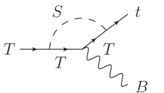
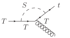
Figure 1: Top partner decay diagrams in the limit that $v\rightarrow 0$ and EW symmetry is restored. Counterterms and external flavor changing self-energies are not shown.

In the limit that $m_{S}\gg m_{T},v$, the scalar $S$ can be integrated out. The lowest dimension operators that contribute to top partner production and decay are the dipole operators:

$$\mathcal{L}_{EFT}=c_{B}\overline{T_{L}}\sigma^{\mu\nu}t_{R}B_{\mu\nu}+c_{G}\overline{T_{L}}\sigma^{\mu\nu}T^{A}t_{R}G^{A}_{\mu\nu}+{\rm h.c.},$$ (22)

where the hypercharge and gluon field strength tensors are

$$B_{\mu\nu} = \partial_{\mu}B_{\nu}-\partial_{\nu}B_{\mu},$$ (23)

$$G_{\mu\nu}^{A} = \partial_{\mu}G^{A}_{\nu}-\partial_{\nu}G^{A}_{\mu}-g_{S}f^{ABC}G^{B}_{\mu}G^{C}_{\nu},$$ (24)

and $f^{ABC}$ is the $SU(3)$ structure constant. These interactions arise from the processes shown in Fig. 1. Taking the limit that $m_{S}\gg m_{T}$ and that EW symmetry is restored ($v\rightarrow 0$, $\sin\theta_{L}\rightarrow 0$), we calculate $T\rightarrow tB$ and $T\rightarrow tg$. The details of the necessary renormalization counterterms can be found in Appendices A and B. Matching onto the EFT, we find the Wilson coefficients:

$$c_{B} = \frac{e}{c_{W}}\frac{2}{3}\frac{\lambda_{1}\lambda_{2}}{24\pi^{2}}\left(1+\frac{3}{4}\ln\frac{m_{T}^{2}}{m_{S}^{2}}\right)\frac{m_{T}}{m_{S}^{2}}$$ (25)

$$c_{G} = g_{S}\frac{\lambda_{1}\lambda_{2}}{24\pi^{2}}\left(1+\frac{3}{4}\ln\frac{m_{T}^{2}}{m_{S}^{2}}\right)\frac{m_{T}}{m_{S}^{2}}.$$ (26)

Note that the ratio of the Wilson coefficients $c_{G}/c_{B}=3\,g_{s}c_{W}/(2\,e)$ is completely determined by the the ratio of the strong and Hypercharge coupling constants. This is because the structure of the loop diagrams in Fig. 1 are essentially the same with the only difference being the external gauge boson and their couplings to the top partner. Also, although the operators in Eq. (22) are dimension five, the Wilson coefficients are suppressed by two powers of $m_{S}$ ($m_{T}/m_{S}^{2}$) and not one power ($1/m_{S}$). The dipole operators couple left- and right-chiral fields. Hence, the loop diagram needs an odd number of changes in chirality. From just the couplings, the diagrams in Fig. 1 have an even number of chiral flips. An additional mass insertion is needed and one power of $m_{T}$ in the numerator is necessary. The operators are then suppressed by $m_{T}/m_{S}^{2}$ and not $1/m_{S}$.

3 Production and Decay of Top Partner

We now discuss the production and decay of the top partner, $T$, in the model presented in Sec. 2. To produce the the numerical results we implement the model in FeynArts Hahn:2000kx via FeynRules Christensen:2008py ; Alloul:2013bka . Matrix element squareds are then generated with FormCalc Hahn:1998yk . We use the NNPDF2.3QED Ball:2013hta parton distribution functions (pdfs) as implemented in LHAPDF6 Buckley:2014ana . We also use the strong coupling constant as implemented in LHAPDF6. Details on the wave-function renormalization and vertex counterterms needed for the calculations in this section can be found in the Appendices A and B.

3.1 Top Partner Production Channels

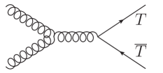
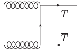
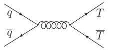
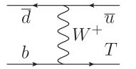
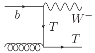
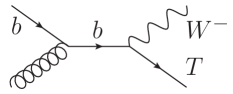
Figure 2: Standard production modes of top partners at the LHC for (a-c) pair production, (d,e) top partner plus jet production, and (f,g) top partner plus $W^{-}$ production. There are conjugate processes for (d-g) that are not shown here.

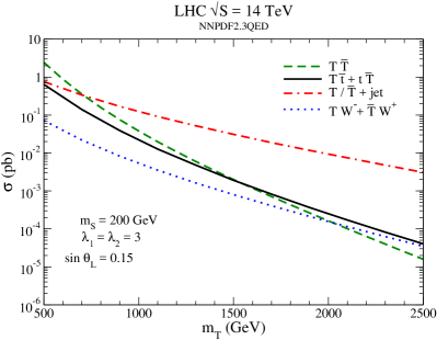
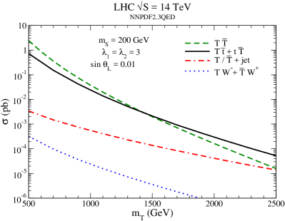
Figure 3: Production cross sections at the $\sqrt{S}=14$ TeV LHC for (green dashed) top partner pair production, (black solid) top partner production in association with a top quark, (red dash-dash-dot) top partner plus jet production, and (blue dotted) top partner plus $W^{\pm}$ production. The parameters are set at a scalar mass $m_{S}=200$ GeV, couplings $\lambda_{1}=\lambda_{2}=3$, and mixing angles (a) $\sin\theta_{L}=0.15$ and (b) $\sin\theta_{L}=0.01$. Factorization, $\mu_{f}$, and renormalization, $\mu_{r}$, scales are set to the sum of the final state particle masses.

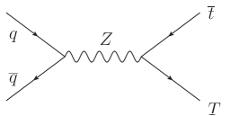
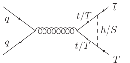
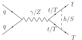
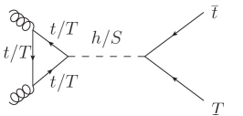
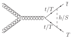
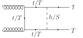
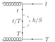
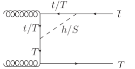
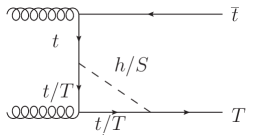
Figure 4: Representative Feynman diagrams for single production of $T$ in association with a top quark for (a) tree level through an $s$-channel $Z$, (b-c) quark-antiquark initial state, and (d-i) gluon fusion. We have not shown the conjugate process, counterterms, off-diagonal self energies of the external top and top partner, or any loops with internal Goldstone bosons, $Z$, or $W^{\pm}$.

There are many possible production channels for top partners. Figure 2 shows the classic tree level mechanisms: (a-c) top partner pair production ($T\overline{T}$), (d,e) top partner plus jet production ($T$+jet), and (f,g) top partner plus $W^{\pm}$ production ($TW$). We collectively refer to final states with a single $T$ produced in association with a SM particle as single top partner production. Although top partner pair production is dominant for much of the parameter region, single top partner plus jet production can become important for very massive $T$ despite the $b$-quark pdf suppression Dolan:2016eki ; Han:2003wu ; Han:2005ru ; Willenbrock:1986cr ; DeSimone:2012fs ; Aguilar-Saavedra:2013qpa ; Backovic:2015bca ; Liu:2016jho . This is mainly due to two effects: the gluon pdf drops precipitously at high mass suppressing the $T\overline{T}$ rate and top partner pair production starts saturating the available LHC phase space at high energies. This can be clearly seen in Fig. 3, which compares the cross sections of various top partner production modes as a function of the top partner mass $m_{T}$. At the $\sqrt{S}=14$ TeV LHC and for a mixing angle of $\sin\theta_{L}=0.15$, Fig. 3, the $T$+jet production becomes larger than that of top partner pair production at a mass around $m_{T}\sim 700$ GeV and $TW$ production is comparable to $T\overline{T}$ production for $m_{T}\sim 2.5$ TeV.

However, for the simplest model where the SM is augmented by a single $SU(2)_{L}$ singlet top partner, single top partner production relies on the $b-W-T$ coupling. This coupling is proportional to the to the $T-t$ mixing angle $\sin\theta_{L}$, as can be seen in Eq. (2.2). Hence, the production cross section is proportional to $\sin^{2}\theta_{L}$ and vanishes as the mixing angle goes to zero. In fact, as shown in Fig. 3, $T\overline{T}$ always dominates $T$+jet and $TW$ for $\sin\theta_{L}=0.01$ at the $\sqrt{S}=14$ TeV LHC for all masses shown.

In the model presented in Sec. 2, in addition to the production modes in Fig. 2, the flavor-off diagonal couplings between the new scalar, top partner, and top quark introduces new loop level production mode: top partner production in association with a top quark ($Tt$). Representative Feynman diagrams with flavor off-diagonal scalar couplings for this process are show in Fig. 4. We do not show the conjugate process; counterterm diagrams; diagrams with Goldstone bosons, $Z$s, or $W^{\pm}$s internal to the loop; or external off-diagonal self-energy diagrams between the top quark and top partner. However, these are included in the calculation. Although $Tt$ production is allowed at tree level for non-zero $\sin\theta_{L}$, as with $T$+jet and $TW$ production, the tree level $Tt$ cross section is proportional to $\sin^{2}\theta_{L}$. Hence, it vanishes as $\sin\theta_{L}$ vanishes. However, the $S-t-T$ and $S-T-T$ couplings do not vanish for $\sin\theta_{L}=0$ and the loop level production survives.

For $m_{S}>m_{T}+m_{t}$, it is possible for the scalar to resonantly decay into the top partner and top through the diagram in Fig. 4. If the scalar is not too heavy, it will be possible to produce it and look for this decay channel at the LHC. This type of signal has been much studied and searched for Fichet:2016xpw ; Greco:2014aza ; Sirunyan:2017bfa ; Dobrescu:2009vz ; Barcelo:2011wu ; Bini:2011zb . However, if the scalar is too heavy it will not be possible to produce it at the LHC. In this case, the EFT presented in Sec. 2.3 is relevant. As can be clearly seen, the production cross section is then suppressed by $1/m_{S}^{4}$. For large scalar masses it is always negligible compared to pair production. Hence, for our discussion of $T$ production we focus on the scenario where $m_{S}<m_{T}+m_{t}$. However, as we will see, for $m_{S}\gg m_{T}$ the decay channels of the top partner are interesting and present a new phenomenology.

The importance of $Tt$ production can be seen in Fig. 3. For $m_{S}=200$ GeV and both $\sin\theta_{L}=0.15$ and $\sin\theta_{L}=0.01$, at the $\sqrt{S}=14$ TeV LHC the top partner plus top production rate is greater than that of top partner pair production for $m_{T}\gtrsim 1.5$ TeV. While for $\sin\theta_{L}=0.15$, $T$+jet production is consistently larger than $Tt$ production, the situation changes drastically for smaller mixing angles. As can be seen by comparing Figs. 3 and 3, the $Tt$ rate does not greatly decrease as $\sin\theta_{L}$ becomes small. Figure 3 shows that $Tt$ is the dominant single top partner production mechanism for small mixing angles.

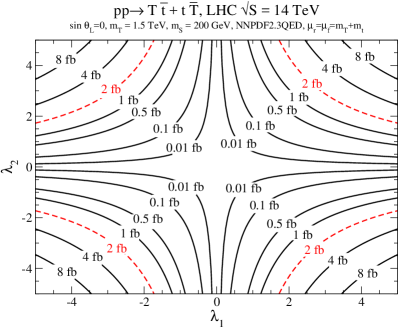
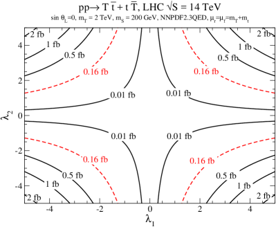
Figure 5: Contours of production cross sections at the $\sqrt{S}=14$ TeV LHC for top partner production in association with a top quark in the $\lambda_{2}-\lambda_{1}$ coupling constant plane for top partner masses (a) $m_{T}=1.5$ TeV and (b) $m_{T}=2$ TeV. The red dashed lines indicate the $T\overline{T}$ production cross section. The other parameters are $m_{S}=200$ GeV and $\sin\theta_{L}=0$. The factorization and renormalization scales are set at $\mu_{r}=\mu_{f}=m_{T}+m_{t}$ for $Tt$ production and $\mu_{r}=\mu_{f}=2m_{T}$ for the $T\overline{T}$ cross section.

In Fig. 5 we show contours of LHC cross sections for top partner plus top production in $\lambda_{1}-\lambda_{2}$ plane in the zero mixing $\sin\theta_{L}=0$ limit. This is presented for both $m_{T}=1.5$ TeV, Fig. 5, and $m_{T}=2$ TeV, Fig. 5. The shapes of the contours can be understood by noting that in the zero mixing limit the $Tt$ production rate is proportional to the coupling constants squared:

$$\sigma(pp\rightarrow T\overline{t}+t\overline{T})\propto\lambda_{1}^{2}\lambda_{2}^{2}$$ (27)

Hence, contours of constant cross section correspond to $|\lambda_{1}|\propto|\lambda_{2}|^{-1}$. For comparison, we also show the top production pair production rate (red dashed lines). As can be seen, there is a significant amount of parameter space for which the $Tt$ rate dominates $T\overline{T}$. Using the simple relation in Eq. (27), for $\sin\theta_{L}=0$ and $m_{S}=200$ GeV, we find that at the $\sqrt{S}=14$ TeV LHC the $Tt$ cross section is larger than the $T\overline{T}$ cross section for

$$\sqrt{|\lambda_{1}\lambda_{2}|} \gtrsim 2.9\quad{\rm for}~{}m_{T}=1.5~{}{\rm GeV~{}and}$$

$$\sqrt{|\lambda_{1}\lambda_{2}|} \gtrsim 2.5\quad{\rm for}~{}m_{T}=2~{}{\rm TeV.}$$ (28)

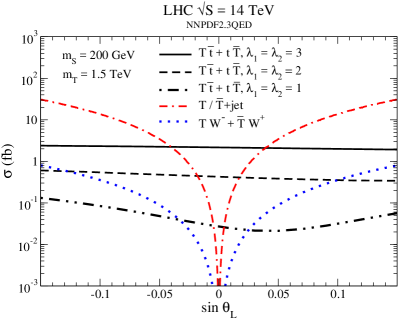
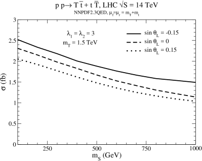
Figure 6: (a) Production cross sections at the $\sqrt{S}=14$ TeV LHC as a function of top partner-top mixing angle $\sin\theta_{L}$ for top partner production in association with a top quark for (black solid) $\lambda_{1,2}=3$, (black dashed) $\lambda_{1,2}=2$, and (black dash-dot-dot) $\lambda_{1,2}=1$. Also shown are (red dash-dash-dot) top partner plus jet production and (blue dotted) top partner plus $W^{\pm}$ production. The top partner mass is $m_{T}=1.5$ TeV and the scalar mass $m_{S}=200$ GeV. (b) Cross sections of top partner production in association with a top partner as a function of the scalar mass $m_{S}$ at the $\sqrt{S}=14$ TeV LHC. The parameters are set at a top partner mass $m_{T}=1.5$ TeV, coupling constants $\lambda_{1,2}=3$, and mixing angle (solid) $\sin\theta_{L}=-0.15$, (dashed) $\sin\theta_{L}=0$, and (dotted) $\sin\theta_{L}=0.15$. For both (a) and (b) the factorization, $\mu_{f}$, and renormalization, $\mu_{r}$, scales are set to the sum of the final state particle masses.

In Fig. 6 we show various single top partner production rates as a function of $\sin\theta_{L}$ for $m_{T}=1.5$ TeV and $m_{S}=200$ GeV. At small mixing angles all the single top partner rates vanish except $Tt$. It is expected that searches for $T$+jet production will limit $\sin\theta_{L}\lesssim 0.02-0.06$ Backovic:2015bca . Hence, this is the parameter region where top partner plus top production is most important. Also, for larger coupling constants $\lambda_{1,2}$, the $Tt$ rate has little dependence on $\sin\theta_{L}$, while for smaller $\lambda_{1,2}$ the dependence is stronger. This can be understood by noting that for non-zero mixing angles, loop diagrams involving the Higgs, $Z$ boson, $W$ boson, and Goldstone bosons contribute to $Tt$. For smaller $\lambda_{1,2}$ these contributions can compete with the scalar $S$ contributions, introducing more $\sin\theta_{L}$ dependence. For larger $\lambda_{1,2}$, the scalar $S$ loops always dominate and mixing angle dependence is milder.

The dependence of the $Tt$ production rate on the scalar mass is shown in Fig. 6 for $\lambda_{1,2}=3$ and $m_{T}=1.5$ TeV. For all mixing angles, the cross section is larger for smaller scalar mass. The dependence of the cross section on $m_{S}$ does not change greatly for different $\sin\theta_{L}$.

3.1.1 Summary

Table 1 summarizes the results of top partner production with $m_{S}=200$ GeV. The left column gives parameter regions for which $Tt$ production is the dominant single top partner production mode. The right column gives parameter regions for which $Tt$ production dominates $T\overline{T}$ double production. For small mixing angles, $Tt$ is the dominant single top production mode, while $Tt$ production dominates $T\overline{T}$ production at large $m_{T}$. Also, $Tt$ production is maximized for smaller scalar masses.

Single Production Double Production $m_{T}=1.5$ TeV, $\lambda_{1,2}=3$, $|\sin\theta_{L}|\lesssim 0.04$ $m_{T}\gtrsim 1.5$ TeV, $\lambda_{1,2}=3$, $\sin\theta_{L}=0$ $m_{T}=1.5$ TeV, $\lambda_{1,2}=2$, $|\sin\theta_{L}|\lesssim 0.02$ $m_{T}=1.5$ TeV, $\sqrt{|\lambda_{1}\lambda_{2}|}\gtrsim 2.9$, $\sin\theta_{L}=0$ $m_{T}=1.5$ TeV, $\lambda_{1,2}=1$, $|\sin\theta_{L}|\lesssim 0.005$ $m_{T}=2$ TeV, $\sqrt{|\lambda_{1}\lambda_{2}|}\gtrsim 2.5$, $\sin\theta_{L}=0$

Table 1: Parameter regions for which $Tt$ production in the dominant single production mode (left column) and $Tt$ production is greater than $T\overline{T}$ pair production (right column) with scalar mass $m_{S}=200$ GeV.

3.2 Top Partner Decay Channels

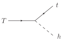
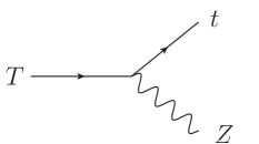
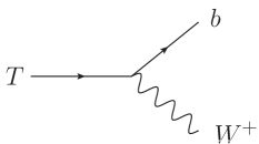
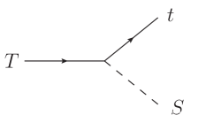
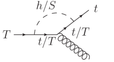
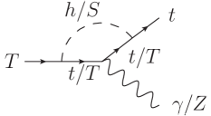
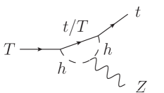
Figure 7: Representative Feynman diagrams for top partner decay at (a-d) tree level and (e-g) one-loop level. Not shown here are external self-energies, external vacuum polarizations, or loops with Goldstone, $W$, or $Z$ bosons.

Figure 7 shows representative Feynman diagrams for top partner decays. Searches for top partners typically rely on the $T\rightarrow th$, $T\rightarrow tZ$, and $T\rightarrow bW$ decays Aaboud:2017zfn ; Aaboud:2017qpr ; Sirunyan:2017pks ; Sirunyan:2017usq as shown in Fig. 7-7. However, in the model presented in Sec. 2, new top partner decay modes are available. For small enough scalar masses, $m_{S}+m_{t}<m_{T}$, there is a new tree level decay $T\rightarrow tS$, as shown in Fig. 7. Additionally, there are possible loop level decays, shown in Figs. 7-7, that are important when the $T\rightarrow tS$ channel is kinematically forbidden and, as we will see, for sufficiently small mixing angle $\sin\theta_{L}$. These new decay channels can change search strategies for fermionic top partners.

Again, in the loop diagrams in Fig. 7, we do not show external self-energies, external vacuum polarizations, loops with $Z$ bosons, loops with $W^{\pm}$ bosons, or loops with Goldstone bosons, although they are included in the calculations. Additionally, we only consider the leading contributions to each decay channel. Hence, $T\rightarrow t\gamma$ and $T\rightarrow tg$ are calculated at one loop. For $T\rightarrow th$ and $T\rightarrow bW$, we only consider tree level decays. While there are loop corrections, for $T\rightarrow th$ they will be dependent on $\lambda_{tt}^{S}$, $\lambda_{TT}^{h}$, $\lambda_{tT}^{h}$, $\lambda_{Tt}^{h}$, $W-b-T$, or the $Z-t-T$ couplings in Eqs. (17-2.2), all of which are proportional to $\sin\theta_{L}$. There is also a diagram proportional to the $S-S-h$ coupling, which we have set to zero. The $S-S-h$ coupling is not technically natural and can be generated through a loop of top quarks and top partners. However, this would would be a two loop contribution to $T\rightarrow th$ and can be safely ignored. Similarly, $T\rightarrow bW$ loop level contributions depend on $\lambda_{tT}^{h}$, $\lambda_{Tt}^{h}$, $\lambda_{TT}^{h}$, $Z-t-T$ or $W-T-b$ couplings in Eqs. (17-2.2), which are also proportional to $\sin\theta_{L}$. Since both the tree and one loop level contributions to $T\rightarrow th$ and $T\rightarrow Wb$ are always proportional to $\sin\theta_{L}$, we expect the tree level diagrams to dominate throughout parameter space and we do not calculate the loop contributions to these decays. The decay $T\rightarrow tZ$ is more complicated. The tree level component vanishes as $\sin\theta_{L}\rightarrow 0$. However, the loop contribution in Fig. 7 does not vanish as $\sin\theta_{L}\rightarrow 0$ since it depends on the $\lambda_{Tt}^{S}$, $\lambda_{TT}^{S}$, and the $Z-T-T$ couplings in Eqs. (18,2.2) which are non-zero for $\sin\theta_{L}=0$. Hence, we calculate tree and loop level diagrams to $T\rightarrow tZ$ so that the dominant contributions are included for all $\sin\theta_{L}$.

3.2.1 $m_{S}<m_{T}-m_{t}$

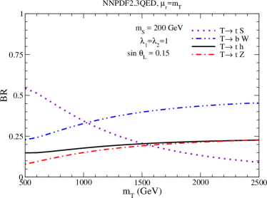
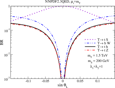
Figure 8: Branching ratios of the top partner as a function of (a) top partner mass and (b) mixing angle $\sin\theta_{L}$ for (violet dotted) $T\rightarrow tS$, (blue dash-dot-dot) $T\rightarrow bW$, (black solid) $T\rightarrow th$, and (red dash-dot) $T\rightarrow tZ$. For (a) the remaining parameters are set at $\lambda_{1,2}=1$, $m_{S}=200$ GeV, and $\sin\theta_{L}=0.15$; while for (b) we have $m_{T}=1.5$ TeV, $m_{S}=200$ GeV, and $\lambda_{1,2}=1$.

We first consider $m_{S}+m_{t}<m_{T}$, where $T\rightarrow tS$ is available. Figure 8 illustrates how the branching ratios of $T$ depend on the top partner mass and mixing angle. Although not shown, we also calculated the branching ratios of $T\rightarrow t\gamma$ and $T\rightarrow tg$, but they are negligible in this regime. As can be seen in Fig. 8, for smaller top partner masses the $T\rightarrow tS$ decay dominates while for larger masses the standard decays $T\rightarrow bW$, $T\rightarrow tZ$, and $T\rightarrow th$ dominate. This can be understood by considering the partial widths in the $m_{T}\gg v,m_{S}$ limit and counting $\sin\theta_{L}\sim m_{t}/m_{T}\sim v/m_{T}$:

$$\Gamma(T\rightarrow tS) = \frac{m_{T}}{32\pi}\left\{\left[\left(\lambda_{tT}^{S}\right)^{2}+\left(\lambda_{Tt}^{S}\right)^{2}\right](1+x_{t}^{2}-x_{S}^{2})+4x_{t}\lambda_{tT}^{S}\lambda_{Tt}^{S}\right\}\lambda^{1/2}(1,x_{t}^{2},x_{S}^{2})$$ (29)

$$\xrightarrow[m_{T}\gg v,m_{S}]{} \frac{\lambda_{1}^{2}m_{T}}{32\pi}$$

$$\Gamma(T\rightarrow th) = \frac{m_{T}}{32\pi}\left\{\left[\left(\lambda_{tT}^{h}\right)^{2}+\left(\lambda_{Tt}^{h}\right)^{2}\right](1+x_{t}^{2}-x_{h}^{2})+4x_{t}\lambda_{tT}^{h}\lambda_{Tt}^{h}\right\}\lambda^{1/2}(1,x_{t}^{2},x_{h}^{2})$$ (30)

$$\xrightarrow[m_{T}\gg v]{} \frac{m_{T}^{3}\sin^{2}\theta_{L}}{32\pi\,v^{2}}$$

$$\Gamma(T\rightarrow tZ) = \frac{g^{2}m_{T}}{512\pi\,c_{W}^{2}}\sin^{2}2\theta_{L}\left\{1+x_{t}^{2}-2\,x_{Z}^{2}+\frac{(1-x_{t}^{2})^{2}}{x_{Z}^{2}}\right\}\lambda^{1/2}(1,x_{t}^{2},x_{Z}^{2})$$ (31)

$$\xrightarrow[m_{T}\gg v]{} \frac{m_{T}^{3}\sin^{2}\theta_{L}}{32\pi\,v^{2}}$$

$$\Gamma(T\rightarrow bW) = \frac{g^{2}m_{T}}{64\pi}\sin^{2}\theta_{L}\left\{1+x_{b}^{2}-2\,x_{W}^{2}+\frac{(1-x_{b}^{2})^{2}}{x_{W}^{2}}\right\}\lambda^{1/2}(1,x_{b}^{2},x_{W}^{2})$$ (32)

$$\xrightarrow[m_{T}\gg v]{} \frac{m_{T}^{3}\sin^{2}\theta_{L}}{16\pi\,v^{2}},$$

where $x_{i}=m_{i}/m_{T}$ and $\lambda(x,y,z)=(x-y-z)^{2}-4\,y\,z$. The decays into SM final states dominate since the partial widths scale as $m_{T}^{3}$ and the partial width $\Gamma(T\rightarrow tS)$ grows as $m_{T}$. This can be understood via the Goldstone Equivalence Theorem and that the $W,Z,h$ couplings are proportional to mass for very heavy $m_{T}$. In fact, the SM decays obey the expectation ${\rm BR}(T\rightarrow bW)\approx 2\,{\rm BR}(T\rightarrow tZ)\approx 2\,{\rm BR}(T\rightarrow th)\approx 50\%$. Of course, allowing mixing between the scalar and Higgs boson will slightly complicate this scenario, since the two mass eigenstate scalars will be superpositions of the gauge singlet scalar and Higgs boson. Since the scalar would then have a component of the Higgs doublet, the parametric dependence of the widths is

$$\Gamma(T\rightarrow tS) \sim \sin^{2}\theta\,\sin^{2}\theta_{L}\frac{m_{T}^{3}}{v^{2}}+\cos^{2}\theta\,\lambda_{1}^{2}m_{T}\quad{\rm and}$$

$$\Gamma(T\rightarrow th) \sim \cos^{2}\theta\sin^{2}\theta_{L}\frac{m_{T}^{3}}{v^{2}}+\sin^{2}\theta\,\lambda_{1}^{2}m_{T},$$ (33)

where $\theta$ is the scalar mixing angle and $m_{T}\gg v,m_{S}$. Then $\Gamma(T\rightarrow tS)$ has a component that grows as $m_{T}^{3}$, but is suppressed by the scalar mixing angle. For simplicity, we are focusing on the scenario where the scalar mixing angle is zero, although, as is clear from Eq. (33), the precise phenomenology will change for non-zero scalar mixing Dolan:2016eki . However, while the branching ratios of the top partner can change, there are no new decay channels for the top partner in the non-zero scalar mixing scenario. Hence, we still capture the major phenomenological aspects of this model.

Precisely when the SM final states dominate will also depend on the coupling constants $\lambda_{1,2}$ and mixing angle $\sin\theta_{L}$. In Fig. 8 we show the dependence of the top partner branching ratios on $\sin\theta_{L}$ for $m_{S}=200$ GeV and $m_{T}=1.5$ TeV. For larger mixing angles $|\sin\theta_{L}|\gtrsim 0.1-0.12$, the decay into bottom quark and $W$ dominates. However, as expected for $\sin\theta_{L}\sim 0$ the branching ratio of $T\rightarrow tS$ is very nearly 100% since the other tree level decay modes vanish.

Figure 9: The scalar $S$ decays into $gg$, $\gamma\gamma$, $\gamma Z$ and $ZZ$ final states through $T$ loop in the zero-mixing limit ($\sin\theta_{L}\rightarrow 0$).

When $T\rightarrow tS$ dominates, search strategies will strongly depend on the decay of the scalar. If $S$ is allowed to have non-negligible mixing with the Higgs boson, the scalar will decay like a heavy Higgs boson. That is, we would expect $S\rightarrow WW$, $S\rightarrow ZZ$, $S\rightarrow tt$, and $S\rightarrow hh$ to be tree level and dominate when they are allowed Dolan:2016eki . If $\lambda_{2}=0$, as-well-as $a_{1}=b_{1}=b_{3}=0$ in Eq. (2), it is possible to apply a $Z_{2}$ symmetry on the top partner and scalar, $T\rightarrow-T$ and $S\rightarrow-S$, while the SM fields are even $SM\rightarrow SM$. The only available decay mode is then $T\rightarrow tS$ and the scalar $S$ is a possible dark matter candidate. Top partners are then pair produced and the signal is $T\bar{T}\rightarrow t\bar{t}+\not{E}_{T}$ Chala:2018qdf . The scenario we consider has no $Z_{2}$ symmetry and sets the scalar-Higgs mixing to zero. Then the only decay channels available to the scalar $S$ are through loops of top quarks and top partners. Depending on the precise mass of the scalar, the decays $S\rightarrow WW$, $S\rightarrow ZZ$, $S\rightarrow\gamma\gamma$, $S\rightarrow Z\gamma$, $S\rightarrow hh$, and $S\rightarrow gg$ will be possible. The $S\rightarrow hh$ and $S\rightarrow WW$ decay rates are mixing angle suppressed since all contributing diagrams are dependent on $\lambda_{Tt}^{h}$, $\lambda_{tT}^{h}$, $\lambda_{TT}^{h}$, $\lambda_{tt}^{S}$, or $W-T-b$ in Eqs. (17-2.2). Hence, in the $\sin\theta_{L}=0$ limit, the scalar $S$ decays to neutral gauge bosons, as shown in Fig. 9, and the branching ratios are determined by the gauge couplings. Then $S\rightarrow gg$ and $T\rightarrow tS\rightarrow tgg$ are by far the dominate decay modes.

3.2.2 $m_{S}>m_{T}-m_{t}$ and Long Lived Top Partners

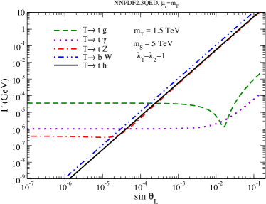
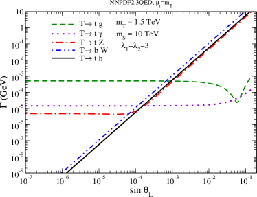
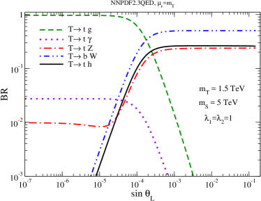
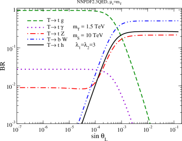
Figure 10: (a,b) Partial widths and (c,d) branching ratios of the top partner for $m_{S}>m_{T}-m_{t}$ for (green dashed) $T\rightarrow tg$, (violet dotted) $T\rightarrow t\gamma$, (red dash-dot) $T\rightarrow tZ$, (blue dash-dot-dot) $T\rightarrow bW$, and (black solid) $T\rightarrow th$. These are shown for top partner mass $m_{T}=1.5$ TeV. The remaining parameters are (a,c) $m_{S}=5$ TeV, $\lambda_{1,2}=1$ and (b,d) $m_{S}=10$ TeV, $\lambda_{1,2}=3$. The renormalization scale is set to the top partner mass.

In Fig. 10 we show the (a,b) total widths and (c,d) branching ratios as a function of mixing angle $\sin\theta_{L}$ for scalar masses larger than top partner mass. The top partner mass is $m_{T}=1.5$ TeV, the scalar masses and couplings are (a,c) $m_{S}=5$ TeV, $\lambda_{1,2}=1$ and (b,d) $m_{S}=10$ TeV, $\lambda_{1,2}=3$. For mixing angle $\sin\theta_{L}\gtrsim 10^{-4}-10^{-3}$, the tree level decays dominate and the partial widths are independent of the scalar mass and couplings. For $\sin\theta_{L}\lesssim 10^{-3}-10^{-4}$ the loop level decay $T\rightarrow tg$ is the main mode. To determine the relative importance of the loop contributions it is useful to look at the $T\rightarrow tZ$ decay channel, since it is the only one for which we include both loop and tree level contributions. At $\sin\theta_{L}\sim 10^{-5}-10^{-4}$ there is a clear transition between a $\Gamma(T\rightarrow tZ)\sim\sin^{2}\theta_{L}$ dependence expected at tree level and a width $\Gamma(T\rightarrow tZ)$ that is relatively independent of $\sin\theta_{L}$. This is the passage between tree level and loop level dominance in $T\rightarrow tZ$.

The dependence of $\Gamma(T\rightarrow tg),\Gamma(T\rightarrow t\gamma),$ and $\Gamma(T\rightarrow tZ)$ on the model parameters at small angles can be understood by noting that for $\sin\theta_{L}\approx 0$, $m_{T}\gg v$, and $m_{S}\gg m_{T}$, the EFT is Eq. (22) is valid. In this EFT, the partial widths are

$$\Gamma_{\rm EFT}(T\rightarrow tg) \approx \frac{\alpha_{s}\,C_{F}\,\lambda_{1}^{2}\lambda_{2}^{2}}{576\,\pi^{4}}\frac{m_{T}^{5}}{m_{S}^{4}}\left(1+\frac{3}{4}\log\frac{m_{T}^{2}}{m_{S}^{2}}\right)^{2}$$ (34)

$$\Gamma_{\rm EFT}(T\rightarrow t\gamma) \approx \frac{\alpha\,\lambda_{1}^{2}\lambda_{2}^{2}}{1296\,\pi^{4}}\frac{m_{T}^{5}}{m_{S}^{4}}\left(1+\frac{3}{4}\log\frac{m_{T}^{2}}{m_{S}^{2}}\right)^{2}$$ (35)

$$\Gamma_{\rm EFT}(T\rightarrow tZ) \approx \frac{\alpha\,\lambda_{1}^{2}\lambda_{2}^{2}\,s_{W}^{2}}{1296\,\pi^{4}\,c_{W}^{2}}\frac{m_{T}^{5}}{m_{S}^{4}}\left(1+\frac{3}{4}\log\frac{m_{T}^{2}}{m_{S}^{2}}\right)^{2}.$$ (36)

Hence, the partial widths are independent of $\sin\theta_{L}$ and all have the same parametric dependence on the top partner mass, scalar mass, and couplings $\lambda_{1,2}$.

The branching ratios of the top partner in the $m_{S}>m_{T}-m_{t}$ regime are shown in Figs. 10 and 10. Although the values of the partial widths depend on the precise model parameters, the branching ratios are largely independent of model parameters for larger $\sin\theta_{L}\gtrsim 10^{-3}$ or small $\sin\theta_{L}\lesssim 10^{-5}$. The behavior of the branching ratios for $\sin\theta_{L}\sim 10^{-5}-10^{-3}$ depends on the relative dominance of the tree level and loop level contribution, and hence the model parameters, as discussed above. For mixing angles $\sin\theta_{L}\gtrsim 10^{-3}$, the tree level decays in to SM EW bosons $T\rightarrow bW$, $T\rightarrow tZ$ and $T\rightarrow th$ dominate and they obey the expected relation ${\rm BR}(T\rightarrow bW)\approx 2\,{\rm BR}(T\rightarrow tZ)\approx 2\,{\rm BR}(T\rightarrow th)\approx 50\%$. This can be understood by noting that in the heavy top partner regime, these partial widths only depend on $\sin\theta_{L}$ and $m_{T}$ and this dependence cancels in the ratios of the widths in Eqs. (30-32).

For $\sin\theta_{L}\lesssim 10^{-4}$ the decay $T\rightarrow tg$ dominates, while for $\sin\theta_{L}\lesssim 10^{-5}$ all loop level decays dominate and the branching ratios are approximately independent of the model parameters. For the EFT, since the partial widths in Eqs. (34-36) have the same parametric dependence, the branching ratios are independent of couplings $\lambda_{1,2}$ and masses $m_{T},m_{S}$. Hence, the branching ratios are largely determined by the gauge coupling constants and weak mixing angle. Then the decay $T\rightarrow tg$ is by far the dominate mode due to the strong coupling constant. There are additional corrections from the Higgs vev to Eq. (22) arising from neglected dimension-6 operators of the form

$$\overline{Q_{L}}\sigma^{\mu\nu}\widetilde{\Phi}T_{R}B_{\mu\nu},\quad\overline{Q_{L}}\sigma^{\mu\nu}\widetilde{\Phi}T^{A}T_{R}G_{\mu\nu}^{A}.$$ (37)

This can explain the $\mathcal{O}(10\%)$ differences between the branching ratios at $m_{S}=5$ TeV and $10$ TeV, as observed in Figs. 10 and 10.

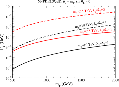
Figure 11: (a) Total width of top partner and (b) decay length of top partner for $\sin\theta_{L}=0$. In both (a,b) the scalar mass is (red) $m_{S}=2.5$ TeV and (black) $m_{S}=10$ TeV. In (a) the coupling constants are (dashed) $\lambda_{1,2}=3$ and (solid) $\lambda_{1,2}=1$. In (b) the coupling constants are (dotted) $\lambda_{1,2}=10^{-3}$, (dashed) $\lambda_{1,2}=10^{-2}$, and (solid) $\lambda_{1,2}=10^{-1}$. The renormalization scale is set to the top partner mass.

For heavy scalars $m_{S}>m_{T}-m_{t}$ and zero mixing angle $\sin\theta_{L}=0$, Fig. 11 shows (a) the total width and (b) the decay length of the top partner for various parameter points. If the decay width of a colored particle is less than $\Lambda_{QCD}\sim 100$ MeV Patrignani:2016xqp , we expect the particle to hadronize and bind with light quarks before it decays. As can be clearly seen, when the loop level decays of the top partner are dominant, we have the total width $\Gamma_{T}<\Lambda_{QCD}$ for the vast majority of parameter space. Hence, the top partner almost always hadronizes before it decays. See for example Ref. Buchkremer:2012dn for a discussion of the phenomenology of top partner hadrons.

At threshold it may be possible for pair produced top partners to bind and form exotic heavy quarkonia, $\eta_{T}=\langle T\overline{T}\rangle$. This will be possible if the decay widths of $T$ and $\eta_{T}$ are less than the binding energy, $E_{b}$, of $\eta_{T}$. If this condition is not satisfied, the lifetime of $\eta_{T}$ will be less than the characteristic orbital time of the constituents and $\eta_{T}$ will not be a resonance. Assuming that the binding force is essentially Coulombic, this condition is Bigi:1986jk ; Kats:2012ym :

$$\Gamma_{T},\Gamma_{\eta_{T}}\lesssim|E_{b}|=\frac{C_{F}^{2}}{4}\alpha_{s}^{2}(m_{T})m_{T}=4~{}{\rm GeV}\left(\frac{\alpha_{s}(m_{T})}{\alpha_{S}(1~{}{\rm TeV})}\right)^{2}\frac{m_{T}}{1~{}\rm TeV},~{}$$ (38)

where $\Gamma_{\eta_{T}}$ is the $\eta_{T}$ decay width. The precise decay pattern of the exotic quarkonia depend on the model parameters. In addition to top partner decays, $\eta_{T}$ has decays into other SM final states. The dominant mode is $\eta_{T}\rightarrow gg$ Buchkremer:2012dn ; Kats:2012ym with partial width $\Gamma(\eta_{T}\rightarrow gg)\sim 1-10$ MeV Barger:1987xg ; Kats:2012ym . Hence, if $\Gamma_{T}\ll\Gamma(\eta_{T}\rightarrow gg)$ the condition to form quarkonia in Eq. (38) is always satisfied. Additionally, we have ${\rm BR}(\eta_{T}\rightarrow gg)\approx 1$ and can employ a typical search for exotic quarkonia Barger:1987xg ; Kats:2012ym ; Buchkremer:2012dn ; Kuhn:1993cp . However, if $|E_{b}|\gtrsim\Gamma_{T}\gtrsim\Gamma(\eta_{T}\rightarrow gg)$, the top partner decays are expected to dominate the $\eta_{T}$ decays. The top partners will decay according to the branching ratios in Fig. 10. For the parameter ranges in Fig. 11, the condition in Eq. (38) is always satisfied.

As can be seen in Fig. 11, for not too small couplings, the decay lengths of the top partners can be significant on the scales of collider experiments. This leads to many exotic phenomena such as displaced vertices Strassler:2006im ; Graham:2012th ; Liu:2015bma , stopped particles Drees:1990yw ; Arvanitaki:2005nq ; Graham:2011ah , and long lived particles Fairbairn:2006gg . The different decay lengths can be categorized as

• Prompt decays: Prompt decays have impact parameters $\lesssim 500~{}\mu$m CMS:2014wda . For $m_{S}=2.5$ TeV, the top partner decays are prompt if $m_{T}\gtrsim$ $200-1000$ GeV and $10^{-1}\gtrsim\lambda_{1,2}\gtrsim 10^{-2}$. For $m_{S}=10$ TeV, the decays are prompt if $m_{T}\gtrsim 300$ GeV and $\lambda_{1,2}\gtrsim 10^{-1}$.

• Displaced vertices: If a particle’s decay length is in the range $\mathcal{O}(1~{}{\rm mm})-\mathcal{O}(1~{}{\rm m})$ it can be reconstructed as a displaced vertex offset from the primary vertex of the proton-proton interaction Liu:2015bma ; CMS:2014wda ; Aad:2015rba ; Khachatryan:2016unx ; Sirunyan:2017jdo ; Aaboud:2017iio ; ATLAS-CONF-2017-026 . The top partner has these decay lengths for the following parameter regions:

  $$\lambda_{1,2} \sim 10^{-3},\quad m_{S}=2.5~{}{\rm TeV},\quad m_{T}\gtrsim 1.5~{}{\rm TeV}$$ (39)

  $$\lambda_{1,2} \sim 10^{-2},\quad m_{S}=2.5~{}{\rm TeV},\quad m_{T}\lesssim 800~{}{\rm GeV}$$ (40)

  $$\lambda_{1,2} \sim 10^{-2},\quad m_{S}=10~{}{\rm TeV},\quad 400~{}{\rm GeV}\lesssim m_{T}\lesssim 2~{}{\rm TeV}$$ (41)

  $$\lambda_{1,2} \sim 10^{-1},\quad m_{S}=10~{}{\rm TeV},\quad m_{T}\lesssim 300~{}{\rm GeV}.$$ (42)

• “Stable” particles: It is possible for charged and colored particles to be stable on collider scales Fairbairn:2006gg . Searches typically look for either high energy deposits in the trackers, measure time of flight with the muon systems, or search for decays in the hadronic calorimeter Aad:2015asa ; ATLAS-CONF-2016-103 ; Chatrchyan:2013oca ; Khachatryan:2016sfv ; ATLAS:2014fka ; Aad:2015qfa ; Aaboud:2016uth . These searches are sensitive to decay lengths of $\mathcal{O}(1~{}{\rm m})-\mathcal{O}(10~{}{\rm m})$ or longer. For both $m_{S}=2.5$ TeV and $10$ TeV, top partners have these decay lengths for $\lambda_{1,2}\lesssim 10^{-3}$ and $m_{T}\lesssim 2$ TeV. For $m_{S}=10$ TeV, top partners also have these decay lengths for $\lambda_{1,2}\sim 10^{-2}$ and $m_{T}\lesssim 400$ GeV.

• Stopped particles: Long lived colored particles hadronize and interact with the detectors, losing energy through ionization Drees:1990yw ; Arvanitaki:2005nq . It is possible for all the energy to be lost and the particles to stop inside the hadronic calorimeter Arvanitaki:2005nq ; Graham:2011ah . For $\mathcal{O}(1~{}{\rm TeV})$ colored particles, nearly 100$\%$ with speeds below $\beta\sim 0.25-0.3$ will stop Arvanitaki:2005nq . If the particle’s lifetime is $\gtrsim~{}\mathcal{O}(100~{}{\rm ns})$, they can be searched for as decays inside the hadronic calorimeter that are out of time with the bunch crossing Graham:2011ah ; Sirunyan:2017sbs ; Khachatryan:2015jha ; Aad:2013gva . For particles to stop in the calorimeter, they must be long lived on collider time scales. Hence, much the same parameter space that gives “stable” particles gives stopped particles.

3.2.3 Summary

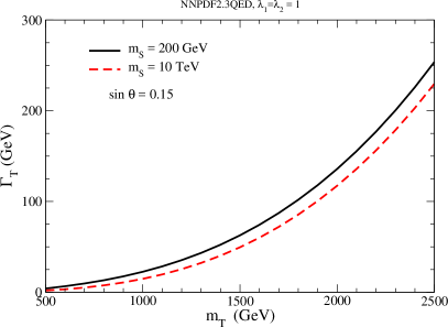
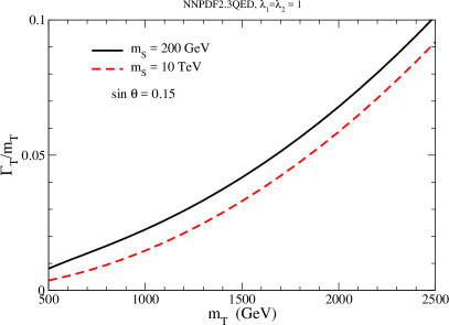
Figure 12: (a) Total width of top partner and (b) width to mass ratio for $\lambda_{1,2}=1$, $\sin\theta_{L}=0.15$, and (black solid) $m_{S}=200$ GeV and (red dashed) $m_{S}=10$ TeV.

In Fig. 12 we show the (a) total width and (b) width to mass ratio for (black solid) $m_{S}=200$ GeV and (red dashed) $m_{S}=10$ TeV with $\sin\theta_{L}=0.15$. For $m_{S}>m_{T}-m_{t}$, the $T\rightarrow St$ decay mode is no longer allowed. However, for non-negligible mixing angle, the tree level $T\rightarrow Wb$, $T\rightarrow tZ$, and $T\rightarrow th$ are still available and growing as $m_{T}^{3}$. The result of decoupling $S$ is to suppress the total width by $\sim 50\%$ for $m_{T}\sim 500$ GeV and $\sim 10\%$ for $m_{T}\sim 2.5$ TeV. For both cases, although the width to Higgs and gauge bosons increases with $m_{T}^{3}$, the width to mass ratio never exceeds $10\%$ and can always be safely regarded as narrow.

$\sin\theta_{L}\sim 0$ $\sin\theta_{L}\sim 0.1$ $m_{S}<m_{T}-m_{t}$ ${\rm BR}(T\rightarrow tS)\approx 1$ ${\rm BR}(T\rightarrow tS)\sim 0.1-0.5\quad{\rm BR}(T\rightarrow bW)\sim 0.25-0.5$ ${\rm BR}(T\rightarrow th)\sim 0.1-0.25\quad{\rm BR}(T\rightarrow tZ)\sim 0.15-0.25$ $m_{S}>m_{T}-m_{t}$ ${\rm BR}(T\rightarrow tg)\approx 1$ ${\rm BR}(T\rightarrow bW)\approx 2\,{\rm BR}(T\rightarrow tZ)\approx 2\,{\rm BR}(T\rightarrow th)\approx 0.5$

Table 2: Branching ratios of dominant top partner decay modes for different mixing angles and mass regions.

$\sin\theta_{L}=0$ $m_{S}=2.5$ TeV $m_{S}=10$ TeV Prompt $\lambda_{1,2}\sim 10^{-1}-10^{-2}$, $m_{T}\gtrsim~{}0.2-1$ TeV $\lambda_{1,2}\gtrsim 10^{-1}$, $m_{T}\gtrsim 300$ GeV Displaced $\lambda_{1,2}\sim 10^{-3}$, $m_{T}\gtrsim 1.5$ TeV $\lambda_{1,2}\sim 10^{-2}$, $400~{}{\rm GeV}\lesssim m_{T}\lesssim 2$ TeV or $\lambda_{1,2}\sim 10^{-2}$, $m_{T}\lesssim 800$ GeV or $\lambda_{1,2}\sim 10^{-1}$, $m_{T}\lesssim 300$ GeV “Stable” $\lambda_{1,2}\lesssim 10^{-3}$, $m_{T}\lesssim 2$ TeV $\lambda_{1,2}\lesssim 10^{-3}$, $m_{T}\lesssim 2$  TeV /Stopped or $\lambda_{1,2}\sim 10^{-2}$, $m_{T}\lesssim 400$ GeV Hadronize Perturbative $\lambda_{1,2}$ Perturbative $\lambda_{1,2}$

Table 3: For $\sin\theta_{L}=0$, Parameter spaces that give us prompt decays, displaced vertices, top partners that are stable on collider time scales, top partners that can stop in the calorimeters, and top partners that hadronize.

We summarize our results for top partner decays in Tables 2 and 3. The possible ranges of the dominant top partner decay modes for different mixing angle and scalar mass ranges are shown in Table 2. In Table 3, we give representative parameter regions that give various collider signatures of long lived top partners.

4 Production and Decay of the Scalar

We now discuss the production and decay of the scalar, $S$, in the model presented in Sec. 2. We focus on the region of parameter space for which the scalar can be produced at the LHC with reasonable rates, i.e. $m_{S}\sim 100s$ GeV and $m_{T}>m_{S}$. As mentioned in the previous section, the scalar can be produced via decays of the top partner. The scalar can also be directly produced through gluon fusion mediated by top quark and top partner loops, similar to the loops in Fig. 9. In Fig. 13, we show the production cross sections for the scalar for various top partner masses and $\lambda_{2}=1$. The scalar-Higgs and top partner-top mixing angles are set to zero. In this limit, only the top partner loops contribute and for $m_{T}\gg m_{S}$ the cross section scales as $\sim\lambda^{2}_{2}/m^{2}_{T}$. Hence, the cross sections for different couplings and top partner masses can be easily obtained by rescaling these results. The cross sections for scalar production are found by rescaling the N³LO scalar gluon fusion production cross sections Anastasiou:2016hlm . That is, we use the relevant Wilson coefficient for the $g-g-S$ contact interaction for $m_{T}\gg m_{S}$.

With $\sin\theta_{L}=0$ and no Higgs-scalar mixing, $S$ can decay into $gg$, $\gamma\gamma$, $\gamma Z$ and $ZZ$ through top partner loops, as shown in Fig. 9. We show the branching ratios of the scalar $S$ in this limit in Fig. 13. For $m_{T}\gg m_{S}$, all partial widths are proportional to $\lambda_{2}^{2}/m^{2}_{T}$. Hence, the branching ratios are independent of the Yukawa coupling $\lambda_{2}$ and the top partner mass, and are determined by ratios of gauge couplings. Due to the strong coupling, the dominant decay mode is into gluons with $\rm{BR}(S\rightarrow gg)\simeq 99\%$.

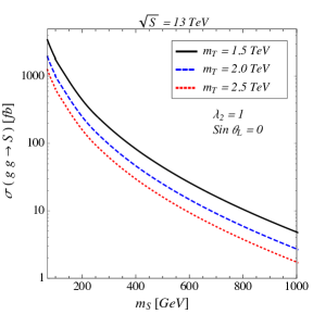
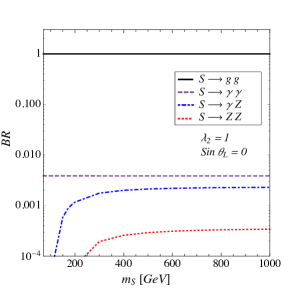
Figure 13: (a) The single $S$ production cross sections via gluon fusion at $\rm{N^{3}LO}$ accuracy in QCD at $\sqrt{S}=13$ TeV for (black solid) $m_{T}=1.5$ TeV, (blue dash) $m_{T}=2$ TeV, and (red dot) $m_{T}=2.5$ TeV. (b) The branching ratios of $S$ decaying into (black solid) $gg$, (violet dash) $\gamma\gamma$, (blue dash-dot) $\gamma Z$, and (red dot) $ZZ$ final states. All plots are made in with zero top partner-top mixing ($\sin\theta_{L}\rightarrow 0$) with $\lambda_{2}=1$.

5 Experimental constraints

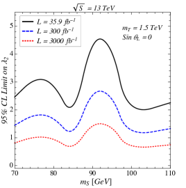
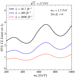
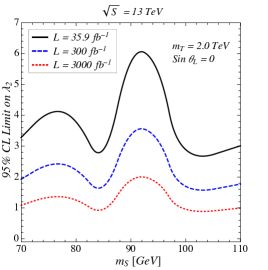
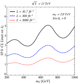
Figure 14: The excluded regions of the parameter space in the (a,c) lower and (b,d) higher mass regions of $S$ for (a,b) $m_{T}=1.5$ TeV and (c,d) $m_{T}=2.0$ TeV. The regions above the black solid line are excluded diphoton searches CMS-PAS-HIG-17-013 ; Aaboud:2017yyg at the 13 TeV LHC. The blue dashed and red dotted curves are the projected exclusions with $300~{}\rm{fb}^{-1}$ and $3000~{}\rm{fb}^{-1}$ luminosities, respectively, via a naive rescaling based on the current limits.

Some of the most constraining limits on colored particles come from QCD pair production shown in Figs. 2-2. The production is mediated by the strong force, and the rate is completely determined by the mass, spin, and color representation of the produced particles. Hence, it is relatively model independent. There have been many searches for top pair production, but their applicability depends on on the precise decay pattern of the top partner. We summarize limits from pair production according to the mass and mixing categories in Table 2:

• $\mathbf{m_{S}>m_{T}-m_{t}}$ and $\mathbf{\sin\theta_{L}\sim 0.1}$: The $T\rightarrow tS$ channel is forbidden, and the classic tree level decays $T\rightarrow th$, $T\rightarrow tZ$, and $T\rightarrow bW$ obey the expected relation ${\rm BR}(T\rightarrow bW)\approx 2\,{\rm BR}(T\rightarrow tZ)\approx 2\,{\rm BR}(T\rightarrow th)\approx 0.5$. For this decay pattern recent studies of ATLAS Aaboud:2017zfn ; Aaboud:2017qpr and CMS Sirunyan:2017pks ; Sirunyan:2017usq excluded $m_{T}\lesssim 1.2-1.3$ TeV.

• $\mathbf{m_{S}<m_{T}-m_{t}}$ and $\mathbf{\sin\theta_{L}\sim 0.1}$: All tree level decays are available: $T\rightarrow tS,\,T\rightarrow th,\,T\rightarrow tZ,$ and $T\rightarrow bW$. The traditional searches for pair produced top partners $T\rightarrow th,\,T\rightarrow tZ$, and $T\rightarrow bW$ Aaboud:2017zfn ; Aaboud:2017qpr ; Sirunyan:2017pks ; Sirunyan:2017usq are then applicable. However, the branching ratios to $th$, $tZ$, and $bW$ do not obey the expected pattern ${\rm BR}(T\rightarrow bW)\approx 2\,{\rm BR}(T\rightarrow tZ)\approx 2\,{\rm BR}(T\rightarrow th)\approx 0.5$, as shown in Table 2 and Fig. 8. Hence, the bounds are weakened. To fill in the gaps, searches for $T\rightarrow tS$ will have to be performed Dolan:2016eki . These will depend on the decay pattern of the scalar $S$, as discussed in Sections 3.2.1 and 4.

• $\mathbf{m_{S}>m_{T}-m_{t}}$ and $\mathbf{\sin\theta_{L}\sim 0}$: All tree level decays are very suppressed, and the loop level decays are relevant: $T\rightarrow tg$, $T\rightarrow t\gamma$, and $T\rightarrow tZ$. A recent CMS analysis Sirunyan:2017yta searched for pair-produced spin 3/2 vector-like excited quarks $T_{3/2}$ which exclusively decays as $T_{3/2}\rightarrow tg$. The lower limit on the mass was found to be $\sim 1.2$ TeV. While ${\rm BR}(T\rightarrow tg)\sim 1$, the pair production rate of $T$ is different from $T_{3/2}$ since $T$ is spin 1/2. We recast the CMS search Sirunyan:2017yta to assess the current constraint on $T$ using NNLO pair production cross section Sirunyan:2017usq ; Czakon:2011xx ; Czakon:2013goa ; Czakon:2012pz ; Czakon:2012zr ; Cacciari:2011hy . The mass bound of this search is then $m_{T}\gtrsim 930$ GeV.

• $\mathbf{m_{S}<m_{T}-m_{t}}$ and $\mathbf{\sin\theta_{L}\sim 0}$: The decay channel $T\rightarrow tS$ dominates with branching ratio ${\rm BR}(T\rightarrow tS)\sim 1$. This decay channel will require new search strategies Dolan:2016eki , which will depend on the decay pattern of the scalar $S$ and whether or not it mixes with the Higgs boson. See Sections 3.2.1 and  4 for a discussion.

To be conservative, we will assume the strongest constraints from pair production and work in the regime $m_{T}\gtrsim 1.2-1.3$ TeV.

An alternative avenue to look for $T$ in the high mass region is the EW single production in association with jets or $W$ Willenbrock:1986cr ; Han:2003wu ; Han:2005ru , as shown in Figs. 2-2. Searches for the single production of $T$ in ATLAS ATLAS-CONF-2016-072 and CMS CMS-PAS-B2G-16-005 ; Sirunyan:2017ynj have excluded $m_{T}\lesssim 1-1.8$ TeV depending on the coupling strengths as well as branching ratios. For the $SU(2)_{L}$ singlet top partner model, this production mechanism vanishes as $\sin\theta_{L}\rightarrow 0$, and the constraints can be avoided.

The most stringent constraints to the mixing between top partners and top quarks comes from EW precision measurements He:2001tp ; Chen:2017hak ; Chen:2014xwa ; Dawson:2012di ; Aguilar-Saavedra:2013qpa . The oblique parameters constrain $|\sin\theta_{L}|\lesssim 0.16$ for $m_{T}=1$ TeV and $|\sin\theta_{L}|\lesssim 0.11$ for $m_{T}=2$ TeV Chen:2017hak ; Dawson:2012di ; Aguilar-Saavedra:2013qpa . The collider bounds are considerably less constraining ATLAS-CONF-2016-072 .

Recent scalar resonance searches at the LHC in the $gg$ CMS-PAS-EXO-16-056 , $\gamma\gamma$ CMS-PAS-HIG-17-013 ; Aaboud:2017yyg , $\gamma Z$ Sirunyan:2017hsb and $ZZ$ Aaboud:2017rel channels can put significant constraints on the scalar mass and couplings. Despite the small branching ratio, the $S\rightarrow\gamma\gamma$ decay channel ($\rm{BR}\simeq 0.4\%$) is the cleanest, setting the most stringent limit on $S$. The experimental results are given for a low mass region $70~{}{\rm GeV}<m_{S}<110~{}{\rm GeV}$ CMS-PAS-HIG-17-013 and a high mass region $200~{}{\rm GeV}<m_{S}$ Aaboud:2017yyg . Figure 14 demonstrates the excluded regions of the parameter space in the (a,c) lower and (b,d) higher $m_{S}$ regions, assuming for (a,b) $m_{T}=1.5$ TeV and (c,d) $m_{T}=2.0$ TeV. Scalar-Higgs and top partner-top mixing angles have been set to zero. The regions above these lines are excluded at the 13 TeV LHC. We show results for the (black solid) current data, and projections to (blue dash) 300 fb^-1 and (red dot) 3 ab^-1. We have assumed both systematic and statistical uncertainties scale as the square root of luminosity. The outlook for the projected limits at the high luminosity-LHC with 3 ab^-1 indicates that $\lambda_{2}$ is expected to be highly constrained $\lambda_{2}\lesssim 1$ for the scalar $S$ mass of $\sim 100-1000$ GeV. The bound can be relaxed as the top partner mass increases, since the cross section decreases as $1/m_{T}^{2}$.

6 Signal Sensitivity at the High Luminosity-LHC

The loop-induced single $T$ production in association with a top quark, as shown in Fig. 4-4, provides an unique event topology, offering useful handles to suppress the SM backgrounds. In this section, we present a detailed collider analysis for the high luminosity-LHC at $\sqrt{S}=14$ TeV with 3 ab^-1 of data, and estimate the sensitivity reach in the final state

$$p~{}p\rightarrow T~{}\overline{t}+t~{}\overline{T}\rightarrow S~{}t~{}\overline{t}\rightarrow g~{}g~{}t~{}\overline{t}\,.$$ (43)

We focus on the $\sin\theta_{L}=0$ limit so that ${\rm BR}(T\rightarrow tS)\approx 1$ and ${\rm BR}(S\rightarrow gg)\approx 1$. Both $gg$- and $q\overline{q}$-initiated processes are taken into account in the analysis. We focus on the semi-leptonic decay of the $t\overline{t}$ system in order to evade a contamination from the QCD multi-jet background.

6.1 Signal Generation

To generate signal events described in Eq. (43), we first implement the EFT in Eq. (22) within the MadGraph5_aMC@NLO Alwall:2014hca framework using FeynRules Christensen:2008py ; Alloul:2013bka . The vertices needed for $T$ and $S$ decays can be conveniently parametrized by the interaction Lagrangian

$$\lambda^{S}_{Tt}S\overline{T}_{L}t_{R}+\lambda^{S}_{tT}S\overline{t}_{L}T_{R}\;+\;\rm{h.c.}$$ (44)

and the effective operator

$$SG^{A}_{\mu\nu}G_{A}^{\mu\nu}.$$ (45)

We use the default NNPDF2.3QED parton distribution function Ball:2013hta with fixed factorization and renormalization scales set to $m_{T}+m_{t}$. At generation level, we require all partons to pass cuts of

$$p_{T}>30~{}{\rm GeV},\quad{\rm and}\quad~{}|\eta|<5,$$ (46)

while leptons are required to have

$$p_{T}^{\ell}>30~{}{\rm GeV}\quad{\rm and}\quad~{}|\eta^{\ell}|<2.5,$$ (47)

where $p_{T}$ are transverse momentum, $\eta$ is rapidity, and $\ell$ indicates leptons. To acquire better statistics in dealing with the SM backgrounds, we demand

$$H_{T}>700{\rm\ GeV},$$ (48)

where $H_{T}$ denotes the scalar sum of the transverse momenta of all final state particles.

We will consider $m_{S}=110~{}{\rm\ GeV}$, $m_{T}=1.5$ TeV and $2$ TeV, and $\sin\theta_{L}=0$. The $\sin\theta_{L}=0$ limit is particularly interesting in this model because the production and decay patterns of the top partner are different from the the traditional approaches, as discussed in Section 3. We use such a small scalar mass so that the production cross section is maximized, as shown in Fig. 6. However, the EFT in Eq. (22) is not valid. Thus, we reweight the matrix element of the EFT by the exact one-loop calculation on an event-by-event basis. We also reweight the events according to the exact branching ratios of the decays $T\rightarrow tS$ and $S\rightarrow gg$. Details of the $T$ production and decay calculation are given in Sections 3.1 and 3.2, respectively, as-well-as the Appendices A and B. Details of the scalar decay can be found in Section 4. The reweighted events are showered and hadronized by PYTHIA6 Sjostrand:2006za and clustered by the FastJet Cacciari:2011ma implementation of the anti-$k_{T}$ algorithm Cacciari:2008gp with a fixed cone size of $r=0.4\;(1.0)$ for a slim (fat) jet. We include simplistic detector effects based on the ATLAS detector performances ATL-PHYS-PUB-2013-004 , and smear momenta and energies of reconstructed jets and leptons according to the value of their energies (see the details in Appendix C).

6.2 Background Generation

Abbreviations	Backgrounds	Matching	$\sigma\cdot{\rm BR(fb)}$
$t\overline{t}$	$t\overline{t}+\rm{jets}$	4-flavor	$2.91\times 10^{3}\;\rm fb$
Single $t$	$tW+\rm{jets}$	5-flavor	$4.15\times 10^{3}\;\rm fb$
	$tq+{\rm jets}$	4-flavor	$77.2\;\rm fb$
$W$	$W+\rm{jets}$	5-flavor	$4.96\times 10^{3}\;\rm fb$
$VV$	$WW+\rm{jets}$	4-flavor	$111\;\rm fb$
	$WZ+\rm{jets}$	4-flavor	$43.5\;\rm fb$

Table 4: The summary of the SM backgrounds after generation level cuts Eqs. (46-48). Matching refers to the either the 4-flavor or 5-flavor MLM matching. $\sigma\cdot\rm BR$ denotes the production cross section (fb) times branching ratios including the top, $W$, and $Z$ decays.

The SM backgrounds are generated by MadGraph5_aMC@NLO at leading order accuracy in QCD at $\sqrt{S}=14$ TeV with the NNPDF2.3QED parton distribution function Ball:2013hta . All events are subject to the cuts in Eqs. (46-48). We use the default variable renormalization and factorization scales. The MLM-matching Mangano:2006rw scheme is used. The matching scales are chosen to be xqcut = 30 GeV and Qcut = 30 GeV for all backgrounds.

The most significant (irreducible) background is semi-leptonic $t\overline{t}+\rm{jets}$ matched up to two additional jets. The relevant EW produced single-top backgrounds are $tW$ and $tq$, where $q$ is a light or $b$-quark. The $tW$-channel is generated with up to three additional jets and one $W$ decays leptonically while the other decays hadronically. The $tq$ channel is generated with up to two additional jets and we only consider a top quark which decays leptonically. Another relevant background includes $W+\rm{jets}$ with up to four additional jets and we only include a leptonically decaying $W$. Much smaller backgrounds include $WW+\rm{jets}$ with up to three additional jets where one $W$ decays leptonically and the other hadronically. Finally, $WZ+\rm{jets}$ sample is generated with up to three additional jets where the $W$ is forced to decay leptonically and the $Z$ hadronically. Although $WW$ and $WZ$ are small compared to the other backgrounds, they are still large compared to the signal. A detailed summary of the backgrounds, the matching schemes, and their cross section after generation level cuts in Eqs. (46-48) is presented in Table. 4. It should be noted that $tW$ is the dominant contribution to single top, whereas Fig. 3 would seem to indicate that $tq$ should be dominant. However, while EW $tq$ is dominant before cuts, the $H_{T}$ cut in Eq. (48) greatly reduces $tq$ and $tW$ becomes the leading contribution.

All background events are fed into PYTHIA6 Sjostrand:2006za for parton showering and hadronization, and then clustered by the FastJet Cacciari:2011ma implementation of the anti-$k_{T}$ algorithm Cacciari:2008gp . We use two cone sizes of $r=0.4$ and $1.0$ for slim and fat jets, respectively. Momenta and energies of reconstructed jets and leptons are smeared in the same way of the signal event to reflect semi-realistic detector resolution effects.

6.3 Signal Selection and Sensitivity

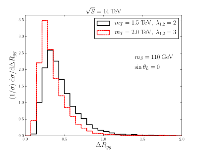
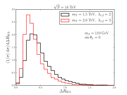
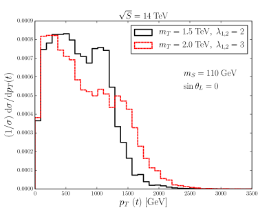
Figure 15: (a) $\Delta R_{gg}$ distribution of the scalar decay products $S\rightarrow gg$. (b) $\Delta R_{Wb}$ distributions between the top quark decay products $t\rightarrow bW$ originating from the top partner decay $T\rightarrow tS$. (c) Transverse momentum distribution of the top quark produced in association with the top partner $pp\rightarrow Tt$. (d) Invariant mass of the top partner and top quark that are produced together $pp\rightarrow Tt$. Distributions are at parton level and for both (black) $m_{T}=1.5$ TeV and (red) $m_{T}=2$ TeV. The other model parameters are set to $m_{S}=110~{}{\rm\ GeV}$ and $\sin\theta_{L}=0$. The coupling constants are $\lambda_{1,2}=2$ for $m_{T}=1.5$ TeV and $\lambda_{1,2}=3$ for $m_{T}=2$ TeV

Since we work in the parameter region that $m_{T}\gg m_{S},m_{t}$, the top quark and $S$ arising from the heavy $T$ decay are kinematically boosted with high $p_{T}$. Hence their decay products are highly collimated. To illustrate this, in Fig. 15 we show $\Delta R_{gg}$ between the two gluons from the $S$ decay, and in Fig. 15 we show $\Delta R_{Wb}$ between the $b$-quark and $W$ from the top quark decay originating from the $T$. These plots are at partonic level before showering, hadronization, or detector effects have been considered. The angular separation $\Delta R_{ij}$ is defined as

$$\Delta R_{ij}=\sqrt{(\Delta\phi_{ij})^{2}+(\Delta\eta_{ij})^{2}},$$ (49)

where $\Delta\phi_{ij}=\phi_{i}-\phi_{j}$ is the difference of the azimuthal angles of particles $i,j$, and $\Delta\eta_{ij}=\eta_{i}-\eta_{j}$ is the difference of the rapidities of the particle $i,j$. As can be seen, the distributions of $\Delta R_{gg}$ and $\Delta R_{Wb}$ peak at $\Delta R_{gg}\sim\Delta R_{Wb}\sim 0.2-0.4$.

The other top quark produced together with $T$ can also acquire a sizable $p_{T}$, as shown in Figs. 15. This can be understood via Fig. 15, where we show the top partner-top invariant mass $m_{Tt}$ distribution at partonic level. In the $\sin\theta_{L}=0$ limit, only loops containing top partners contribute to $pp\rightarrow Tt$. When $m_{Tt}\sim 2m_{T}$, the internal top partners can go on-shell, giving rise to the peaks in the $m_{Tt}$ distributions. These peaks are quite pronounced. Hence, there is a relatively strong Jacobian peak at $p_{T}\sim m_{T}$, causing the shoulder features in Fig. 15.

Since both tops and scalar are all boosted, we require that after showering, hadronization, and detector effects are accounted for that events contain at least one $r=1.0$ fat jet with

$$p_{T}^{j}>400{\rm\ GeV}\quad{\rm and}\quad|\eta^{j}|<2.5.$$ (50)

The variable $r$ describes the cone-size of the anti-$k_{T}$ clustering algorithm Cacciari:2008gp , as described in Sections 6.1 and 6.2. Additionally, our signal consists of one leptonically decaying top $t\rightarrow b\ell\nu$. Hence, we require that our events have missing transverse energy

$$\not{E}_{T}>20{\rm\ GeV},$$ (51)

at least one $r=0.4$ slim jet with

$$p_{T}^{j}>30{\rm\ GeV}\quad{\rm and}\quad|\eta^{j}|<2.5,$$ (52)

and exactly one isolated lepton passing the cuts in Eq. (47) and

$$\mathit{mini-iso}>0.7.$$ (53)

The mini-iso Rehermann:2010vq observable is defined as $p_{T}$ of a lepton divided by the total scalar sum of all charged particles’ transverse energy (including the lepton) with $p_{T}>1{\rm\ GeV}$ in the cone of radius $\Delta R=10{\rm\ GeV}/p_{T}^{\ell}$.

Since both tops are highly boosted the signal contains a fat jet originating from a top quark. Additionally, we have a fat jet originating from the decay of the scalar. Both these fat jets will have unique internal substructures due to the daughter particles. Such events are rare in the SM, and therefore serve as good handles to disentangle the SM backgrounds from our signal events. We use the TemplateTagger v.1.0 Backovic:2012jk implementation of the Template Overlap Method (TOM) Almeida:2010pa ; Backovic:2013bga to tag massive boosted objects. The TOM is based on an overlap $Ov_{i}^{a}$, where $a$ is a parent particle and $i$ is the number of daughter particles inside a fat jet. The closer $Ov_{i}^{a}$ is to one, the more likely that a fat jet originated from the particle $a$. This method is flexible enough to tag any type of heavy object and is weakly susceptible to pileup contamination Backovic:2013bga . A multi-dimensional TOM analysis Backovic:2014ega ; Backovic:2015bca extends its capability to further unravel multiple boosted objects with different internal substructures, and significantly improves a net tagging efficiency of the hadronically-decaying top and scalar $S(\rightarrow gg)$ jets in the same event. For a precise definition see Refs. Almeida:2010pa ; Backovic:2013bga ; Backovic:2012jk . For a $r=1.0$ fat jet to be tagged as the hadronic top, we demand a three-pronged top template overlap score

$$Ov_{3}^{t}>0.6.$$ (54)

We define a fat jet to be an $S$-candidate if it passes a two-pronged $S$ template overlap score and is not tagged as a top-fat jet:

$$Ov_{2}^{S}>0.5\quad{\rm and}\quad Ov_{3}^{t}<0.6.$$ (55)

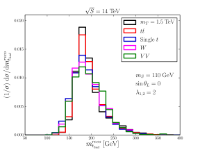
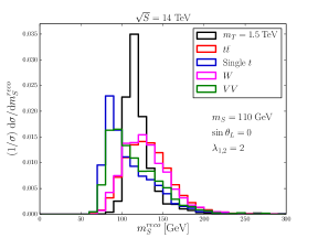
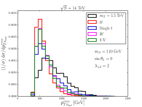
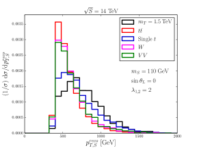
Figure 16: Reconstructed invariant mass distributions of the (a) top-tagged fat jet and (b) scalar-tagged fat jet for $m_{T}=1.5{\rm\ TeV}$. The corresponding $p_{T}$ distributions are shown in (c) and (d) together with background distributions. All plots are generated based on events after showering, hadronization, and detector effects. Our model parameters are $m_{S}=110~{}{\rm\ GeV}$, $\lambda_{1,2}=2$ and $\sin\theta_{L}=0$. Basic cuts in Eqs. (50-53) have been applied.

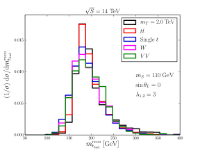
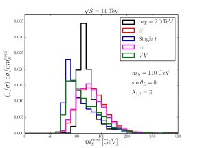
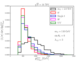
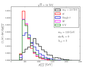
Figure 17: Reconstructed invariant mass distributions of the (a) top-tagged fat jet and (b) scalar-tagged fat jet for $m_{T}=2{\rm\ TeV}$. The corresponding $p_{T}$ distributions are shown in (c) and (d) together with background distributions. All plots are generated based on events after showering, hadronization, and detector effects. Our model parameters are $m_{S}=110~{}{\rm\ GeV}$, $\lambda_{1,2}=3$ and $\sin\theta_{L}=0$. Basic cuts in Eqs. (50-53) have been applied.

Figures 16 and 16 show the resulting reconstructed invariant mass distributions of the top-tagged fat jet, $m_{t_{had}}^{reco}$, and the scalar-tagged fat jet, $m_{S}^{reco}$, respectively, for $m_{T}=1.5{\rm\ TeV}$ for both signal and background. Both the signal and $t\bar{t}$ background $m_{t_{had}}^{reco}$ distributions are highly peaked at the top mass $m_{t}=173$ GeV, while the single top and vector boson backgrounds are not quite as peaked. However, the reconstructed scalar mass $m_{S}^{reco}$ provides more separation from background. For the signal, the $m_{S}^{reco}$ distribution is highly peaked at the scalar mass $m_{S}=110$ GeV, while the background is not. Hence, for $m_{T}=1.5$ TeV we apply the cuts

$$145~{}{\rm GeV}< m_{t_{had}}^{reco} <250~{}{\rm GeV}\quad{\rm and}$$ (56)

$$105~{}{\rm GeV}< m_{S}^{reco} <122~{}{\rm GeV}.$$ (57)

Figures 16 and 16 show the transverse momentum distribution of the top-tagged fat jet and scalar-tagged fat jet, respectively. As can be clearly seen, the signal is harder than the background. For $m_{T}=1.5$ TeV we place the further cut on the reconstructed scalar transverse momentum

$$p^{reco}_{T,S}>540~{}{\rm GeV}.$$ (58)

Finally, since the top-tagged fat jet should contain a $b$-quark, at least one $b$-tagged slim $r=0.4$ jet should be found inside the top-tagged fat jet. We require that exactly one top-tagged fat jet passes the cut in Eq. (56) and has a $b$-tagged slim jet inside, and exactly one scalar-tagged fat jet passes the cuts in Eqs. (57) and (58):

$$N^{1.5}_{t_{had}}=1\quad{\rm and}\quad N^{1.5}_{S}=1,\,{\rm respectively.}$$ (59)

Table 5 is a cut-flow table showing the cumulative effects of cuts on signal and background rates. Relative to the basic cuts in Eqs.(50-53), under the requirement that $N_{t_{had}}^{1.5}=N_{S}^{1.5}=1$, the signal efficiency is $5.8\%$, while the major backgrounds $t\overline{t}$ and single $t$ have efficiencies of $0.085\%$ and $0.057\%$, respectively. The $W$ and $VV$ backgrounds are cut down to $0.0036\%$ and $0.0028\%$, respectively, greatly diminishing the overall size of backgrounds.

For $m_{T}=2$ TeV, the reconstructed invariant mass and transverse momentum distributions for the top-tagged and scalar-tagged fat jets are shown in Fig. 17. The observations for $m_{T}=2$ TeV are largely the same as for $m_{T}=1.5$ TeV, except the $p_{T}$ spectrum of the top-tagged and scalar-tagged fat jets are harder for the signal. Hence, for the targeted $m_{T}=2.0{\rm\ TeV}$ analysis, we slightly tighten the $m_{t_{had}}^{reco}$ mass window

$$155~{}{\rm GeV}<m_{t_{\rm{had}}}^{reco}<250~{}{\rm GeV}.~{}$$ (60)

For the scalar-tagged fat jet we use the same mass window as Eq. (57), but harden the transverse momentum cut:

$$p_{T,S}^{reco}>560~{}{\rm GeV}$$ (61)

However, as the $T$ mass scale increases, we confront the challenge that the signal cross section steeply decreases, weakening our significance. To retain more signal events, we do not require that a $b$-tagged slim jet be found inside the top-tagged fat jet. Hence, for $m_{T}=2$ TeV we require exactly one top-tagged fat jet that passes the cut in Eq. (60) and without the $b$-tagging requirement, and exactly one scalar-tagged fat jet that passes the cuts in Eqs. (57) and (61):

$$N^{2.0}_{t_{had}}=1\quad{\rm and}\quad N^{2.0}_{S}=1,\,{\rm respectively.}$$ (62)

As can be seen in Table 5, due to the relaxation of the $b$-tagging requirement, all efficiencies for background and signal are larger as compared to the $m_{T}=1.5$ TeV case. However, the backgrounds are still efficiently suppressed, especially the backgrounds that do not contain top quarks.

To further separate signal from background, it is useful to fully reconstruct the event. However, this means reconstructing the leptonically decaying top, $t_{lep}$, and the missing neutrino momentum. First, to help reconstruct the top quark, we require that at least one of the slim jets passing the cuts in Eq. (52) is also tagged as a $b$-jet and meets the endpoint criteria

$$m_{b\ell}<153.2+\Gamma{\rm\ GeV}$$ (63)

where $m_{b\ell}$ is the invariant mass of the $b$-tagged slim jet and isolated lepton, and $\Gamma$ is a headroom to take into account effects of parton showering and hadronization. We choose ${\Gamma=20{\rm\ GeV}}$ to keep signal events up to $\sim 90\%$. We then reconstruct the momentum of the missing neutrino following the prescription in Ref. Barger:2006hm ; Gopalakrishna:2010xm . The total transverse momentum of the system is zero, so the transverse momentum of neutrino is just the missing transverse momentum. However, the longitudinal component of the neutrino momentum is still unknown and cannot be determined via momentum conservation since the longitudinal momentum of the initial state is unknown at hadron colliders. We will use the on-shell mass constraints that the invariant mass of the neutrino is $p_{\nu}^{2}=0$ and the invariant mass of the isolated lepton and neutrino satisfy $m^{2}_{\ell\nu}=m^{2}_{W}$. Since these are quadratic equations, there are two possible solutions for the neutrino longitudinal momentum

$$p^{\nu}_{L}=\frac{1}{2~{}(p^{\ell}_{T})^{2}}\Bigg{(}A~{}p^{\ell}_{L}\pm|\vec{p}_{\ell}|~{}\sqrt{A^{2}-4\,\left(p^{\ell}_{T}\right)^{2}\,\not{E}^{2}_{T}}\Bigg{)}\;,$$ (64)

where $A=m^{2}_{W}+2\vec{p}^{\;\ell}_{T}\cdot\vec{\not{E}}_{T}$, $p^{\ell}_{L}$ is the lepton longitudinal momentum, $\vec{p}_{\ell}$ is the lepton’s three-momentum, $\vec{p}_{T}^{\;\ell}$ is the lepton’s transverse momentum vector, and $\vec{\not{E}}_{T}$ is the missing transverse energy vector. To break the two fold-ambiguity of Eq. (64) and to determine which $b$-jet originates from the leptonically decay top, we use the top quark mass constraint. We select the $b$-jet and $p_{L}^{\nu}$ pair that minimizes the quantity

$$|m^{2}_{b\ell\nu}-m^{2}_{t}|$$ (65)

where $m_{b\ell\nu}$ is the invariant mass of a $b$-jet, lepton, and neutrino system. The resulting $b$-jet and neutrino momentum are used to reconstruct the leptonically decaying top, $t_{lep}$. Once we have reconstructed the leptonically decay top, we require that it has the correct mass and has fairly high $p_{T}$:

$$150~{}{\rm GeV}< m^{reco}_{t_{lep}} <210~{}{\rm GeV},\quad p_{T,t_{lep}}^{reco}>500~{}{\rm GeV},\quad{\rm for}\,m_{T}=1.5~{}{\rm TeV},\,{\rm and}$$ (66)

$$150~{}{\rm GeV}< m^{reco}_{t_{lep}} <220~{}{\rm GeV},\quad p_{T,t_{lep}}^{reco}>680~{}{\rm GeV},\quad{\rm for}\,m_{T}=2~{}{\rm TeV}.$$ (67)

As we can see from the fourth rows of Table 5, as compared to the $N_{t_{had}}$ and $N_{S}$ cuts, after $t_{lep}$ reconstruction the vector boson backgrounds are reduced by $2-5$ orders of magnitude, the single top background efficiency is $1-4\%$, and the $t\bar{t}$ efficiency is $1-7\%$. The signal efficiency is $20-40\%$.

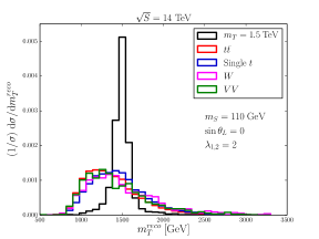
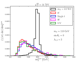
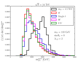
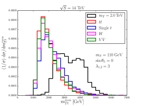
Figure 18: The reconstructed $T$ invariant mass $m_{T}^{reco}$ distributions are shown for (a) $m_{T}=$ 1.5 TeV and (b) 2 TeV. The reconstructed system invariant mass $m_{Tt}^{reco}$ distributions are shown for (c) $m_{T}=$ 1.5 TeV and (d) 2 TeV. All plots are generated based on events after showering, hadronization, and detector effects. The other model parameters are set to $m_{S}=110~{}{\rm\ GeV}$ and $\sin\theta_{L}=0$. The coupling constants are $\lambda_{1,2}=2$ for $m_{T}=1.5$ TeV and $\lambda_{1,2}=3$ for $m_{T}=2$ TeV. Basic cuts in Eqs. (50-53) have been applied.

Although the background is greatly reduced, to suppress it further relative to signal we will use the reconstructed top partner mass $m_{T}^{reco}$ and the total invariant mass of the reconstructed system. While the top quarks and scalar are fully reconstructed, it is not clear yet which top quark originated from the top partner decay. We select the pair $\{S,t_{i}\}$, where $i=had,lep$ denotes either the hadronic or leptonic top, that best reconstructs $T$ by minimizing the mass asymmetry variable

$$\Delta_{m}=\Bigg{|}\frac{m_{T}-m^{reco}_{St_{i}}}{m_{T}+m^{reco}_{St_{i}}}\Bigg{|}~{}\;,$$ (68)

for each mass point $m_{T}=1.5$ and $2~{}{\rm\ TeV}$, where $m^{reco}_{St_{i}}$ stands for the invariant mass of the pair $\{S,t_{i}\}$. The resulting reconstructed top partner invariant mass, $m_{T}^{reco}$, distributions are shown in Figs. 18 and 18 for $m_{T}=1.5$ TeV and $m_{T}=2$ TeV, respectively. They clearly peak at the truth level top partner invariant mass. Hence, we apply the cuts

$$1400~{}{\rm GeV}< m_{T}^{reco} <1550~{}{\rm GeV}\quad{\rm for}\,m_{T}=1.5~{}{\rm TeV}\,{\rm and}$$ (69)

$$1860~{}{\rm GeV}< m_{T}^{reco} <2100~{}{\rm GeV}\quad{\rm for}\,m_{T}=2~{}{\rm TeV}.$$ (70)

One of the compelling features of the loop-induced single production channel is that the reconstructed system invariant mass $m^{reco}_{Tt}$ distribution retains the peak-like structures at high invariant mass. We show this in Figs. 18 and 18 for $m_{T}=1.5$ TeV and $2$ TeV, respectively. Since the backgrounds are peaked at much lower invariant mass, they can be further suppressed with the cuts

$$2865~{}{\rm GeV} < m_{Tt}^{reco}\quad{\rm for}\,m_{T}=1.5~{}{\rm TeV}\,{\rm and},$$ (71)

$$3000~{}{\rm GeV} < m_{Tt}^{reco}\quad{\rm for}\,m_{T}=2~{}{\rm TeV}.$$ (72)

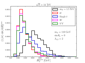
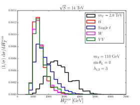
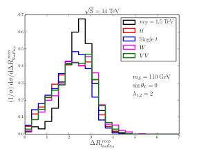
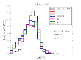
Figure 19: (a,b) $H_{T}^{reco}$, Eq. (73), distributions are shown for (a) $m_{T}=1.5$ TeV and (b) $m_{T}=2$ TeV. (c,d) Distributions of the angular separation between the two reconstructed top quark, $\Delta R^{reco}_{t_{had}t_{lep}}$ are shown for (c) $m_{T}=1.5$ TeV and (d) $m_{T}=2$ TeV. All plots are generated based on events after showering, hadronization, and detector effects. The other model parameters are set to $m_{S}=110~{}{\rm\ GeV}$ and $\sin\theta_{L}=0$. The coupling constants are $\lambda_{1,2}=2$ for $m_{T}=1.5$ TeV and $\lambda_{1,2}=3$ for $m_{T}=2$ TeV. Basic cuts in Eqs. (50-53) have been applied.

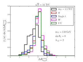
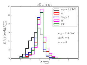
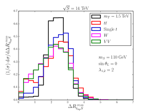
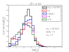
Figure 20: Distributions of the angular separation between (a,b) the reconstructed $S$ and hadronically decaying top, $\Delta R^{reco}_{t_{had}S}$, and (c,d) the reconstructed $S$ and leptonically decaying top, $\Delta R^{reco}_{t_{lep}S}$, for (a,c) $m_{T}=1.5$ TeV and (b,d) $m_{T}=2$ TeV. All plots are generated based on events after showering, hadronization, and detector effects. The other model parameters are set to $m_{S}=110~{}{\rm\ GeV}$ and $\sin\theta_{L}=0$. The coupling constants are $\lambda_{1,2}=2$ for $m_{T}=1.5$ TeV and $\lambda_{1,2}=3$ for $m_{T}=2$ TeV. Basic cuts in Eqs. (50-53) have been applied.

The effects of the the cuts in Eqs. (69-72) on signal and background are shown in the fifth and sixth rows of Table 5. After these cuts the background and signal rates are comparable. However, one final set of cuts is made to increase the significance of the signal. We introduce a variable $H^{reco}_{T}$ defined as the scalar sum of the transverse momenta of the reconstructed top quarks and scalar

$$H^{reco}_{T}=p_{T,t_{had}}^{reco}+p_{T,t_{lep}}^{reco}+p_{T,S}^{reco}\;.$$ (73)

As demonstrated in Figs. 19 and 19 for $m_{T}=$ 1.5 TeV and 2 TeV, respectively, the signal is much harder than the background.

Additionally, individual angular distance variables between the reconstructed tops and scalar $\Delta R^{reco}_{t_{{had}}t_{{lep}}}$, $\Delta R^{reco}_{t_{{had}}S}$ and $\Delta R^{reco}_{t_{{lep}}S}$ deliver additional handles in shaping and controlling the signal region. This is shown in Figs. 19, 19, and 20, where background and signal clearly populate different regions of phase space. Based on these observations, we apply a final set of cuts

$$\left.\begin{aligned} &2050~{}{\rm GeV}<H_{T}^{reco}\\ &\Delta R^{reco}_{t_{had}S}<3.41\\ &1.63<\Delta R_{t_{lep}S}^{reco}\end{aligned}\right\}\quad{\rm for}\,m_{T}=1.5~{}{\rm TeV}\,{\rm and}$$ (74)

$$\left.\begin{aligned} &2050~{}{\rm GeV}<H_{T}^{reco}\\ &1.79<\Delta R^{reco}_{t_{had}t_{lep}}\\ &1.58<\Delta R^{reco}_{t_{had}S}<3.6\\ &1.6<\Delta R_{t_{lep}S}^{reco}<3.1\end{aligned}\right\}\quad{\rm for}\,m_{T}=2~{}{\rm TeV}.$$ (75)

As shown in the last row of the tables in Table 5, these final cuts decrease the background cross section to below the signal rate, with good signal efficiency.

To quantify the observability of our signal at the LHC, we compute a significance ($\sigma$) using the likelihood-ratio method Cowan:2010js

$$\sigma\equiv\sqrt{-2\,\ln\bigg{(}\frac{L(B|Sig\!+\!B)}{L(Sig\!+\!B|Sig\!+\!B)}\bigg{)}}\;\;\;\;\;\text{with}\;\;\;L(x|n)=\frac{x^{n}}{n!}e^{-x}\,,$$ (76)

where $Sig$ and $B$ are the expected number of signal and background events, respectively. All significances in Table 5 are calculated for given luminosity of $3$ ab^-1 and given in the last row. While the cuts from the basic to the reconstructed invariant mass $m_{Tt}^{reco}$ in Eqs. (50-72) decrease background rates until they are comparable to signal, it is the final cuts in Eqs. (74) and (75) that significantly increase the significance. The final signal significance turns out to be $5.0$ for the benchmark parameter point $m_{T}=1.5$ TeV, $\lambda_{1,2}=2$, $m_{S}=110~{}{\rm\ GeV}$ and $\sin\theta_{L}=0$ assuming a luminosity of $3$ ab^-1. Although we can achieve the high significance, only $\sim 1.7$ signal events are expected. While this may be enough to set constraints on the model, it is not enough for discovery. The sensitivity for heavier $T$ mass scales become weaker, where the final signal significance turns out to be $1.9$ for the benchmark parameter point $m_{T}=2.0$ TeV, $\lambda_{1,2}=3$, $m_{S}=110~{}{\rm\ GeV}$ and $\sin\theta_{L}=0$ with the same amount of the luminosity. However, due to relaxation of $b$-tagging inside the hadronically decay top quark fat jet, we actually expect 2.4 signal events, more than $m_{T}=1.5$ TeV.

$m_{T}=1.5$ TeV, $\lambda_{1,2}=2$ Signal [fb] $t\overline{t}$ [fb] Single $t$ [fb] $W$ [fb] $VV$ [fb] $\sigma$ Basic cuts, Eqs. (50-53) $0.055$ $1.3\times 10^{3}$ $2.8\times 10^{3}$ $2.7\times 10^{3}$ $88$ 0.036 $N^{1.5}_{t_{had}}=N^{1.5}_{S}=1$, Eqs. (56-59) $3.2\times 10^{-3}$ 1.11 1.6 0.098 $2.5\times 10^{-3}$ 0.11 Reconstructed $t_{lep}$, Eq. (66) $1.2\times 10^{-3}$ 0.073 0.070 $4.7\times 10^{-4}$ $\ll\mathcal{O}(10^{-5})$ 0.17 $1400~{}{\rm GeV}<m^{reco}_{T}<1550$ GeV, $9.2\times 10^{-4}$ 0.015 $9.4\times 10^{-3}$ $\ll\mathcal{O}(10^{-5})$ $\ll\mathcal{O}(10^{-5})$ 0.32 Eq. (69) $2865{\rm\ GeV}<m_{Tt}^{reco}$, Eq. (71) $6.3\times 10^{-4}$ $1.5\times 10^{-3}$ $7.2\times 10^{-5}$ $\ll\mathcal{O}(10^{-5})$ $\ll\mathcal{O}(10^{-5})$ 0.81 $2050{\rm\ GeV}<H^{\rm reco}_{T}$ $5.8\times 10^{-4}$ $\ll\mathcal{O}(10^{-5})$ $\ll\mathcal{O}(10^{-5})$ $\ll\mathcal{O}(10^{-5})$ $\ll\mathcal{O}(10^{-5})$ 5.0 $\Delta R^{reco}_{t_{{had}}S}<3.41$, Eq. (74) $1.63<\Delta R^{reco}_{t_{{lep}}S}$

$m_{T}=2.0$ TeV, $\lambda_{1,2}=3$ Signal [fb] $t\overline{t}$ [fb] Single $t$ [fb] $W$ [fb] $VV$ [fb] $\sigma$ Basic cuts, Eqs. (50-53) $0.040$ $1.3\times 10^{-3}$ $2.8\times 10^{-3}$ $2.7\times 10^{-3}$ $88$ 0.027 $N_{t_{\rm had}}^{2.0}=N_{S}^{2.0}=1$, Eqs.(57,60-62) $5.4\times 10^{-3}$ 3.0 14 4.3 0.21 0.089 Reconstructed $t_{lep}$, Eq. (67) $1.2\times 10^{-3}$ 0.043 0.096 $8.7\times 10^{-5}$ $6.8\times 10^{-6}$ 0.17 $1860~{}{\rm GeV}<m^{reco}_{T}<2100$ GeV, $1.1\times 10^{-3}$ 0.010 $6.8\times 10^{-3}$ $\ll\mathcal{O}(10^{-5})$ $6.8\times 10^{-6}$ 0.44 Eq. (70) $3000{\rm\ GeV}<m^{reco}_{Tt}$, Eq. (72) $9.4\times 10^{-4}$ $6.9\times 10^{-3}$ $6.8\times 10^{-3}$ $\ll\mathcal{O}(10^{-5})$ $3.4\times 10^{-6}$ 0.43 $2050{\rm\ GeV}<H^{\rm reco}_{T}$ $8.1\times 10^{-4}$ $3.2\times 10^{-4}$ $\ll\mathcal{O}(10^{-5})$ $\ll\mathcal{O}(10^{-5})$ $\ll\mathcal{O}(10^{-5})$ 1.9 $1.79<\Delta R^{reco}_{t_{{had}}t_{{lep}}}$, Eq. (75) $1.58<\Delta R^{reco}_{t_{{had}}S}<3.6$ $1.6<\Delta R^{reco}_{t_{{lep}}S}<3.1$

Table 5: Cumulative cut-flow tables showing the SM background and signal cross sections at two benchmark parameter points (top) $m_{T}=1.5$ TeV and $\lambda_{1,2}=2$ and (bottom) $m_{T}=2.0$ TeV and $\lambda_{1,2}=3$ where we fixed other parameters to $m_{S}=110~{}{\rm\ GeV}$, $\sin\theta_{L}=0$. Significances ($\sigma$) are calculated based on the likelihood-ratio method defined in Eq.(76) for given luminosity of $3$ ab^-1. A summary of the backgrounds can be found in Table 4.

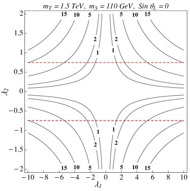
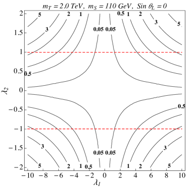
Figure 21: Contours of constant significance, Eq. (76), for two benchmark $T$ mass scales (a) $m_{T}=1.5$ TeV and (b) $m_{T}=2.0$ TeV assuming a luminosity of 3 ab^-1. We set other parameters to $m_{S}=110~{}{\rm\ GeV}$ and $\sin\theta_{L}=0$. The dashed red lines illustrate the bounds coming from the diphoton resonance searches as presented in Fig. 14.

From these results, we can project sensitivities for many coupling constants. For $\sin\theta_{L}=0$, the production cross section is proportional to $\lambda_{1}^{2}\lambda_{2}^{2}$, Eq. (27). Additionally, the branching ratio of $T\rightarrow tS$ is essentially one. Hence, we can simply scale the signal cross sections in Table 5 to determine significances for different coupling constants. In Fig. 21, we summarize the final significance contours for two benchmark $T$ masses (a) $m_{T}=1.5$ TeV and (b) $m_{T}=2.0$ TeV, $m_{S}=110$ GeV, and $\sin\theta_{L}=0$. These are for 3 ab^-1 of data. The solid black lines are contours of constant significance. The dashed red lines illustrate the bounds coming from the diphoton resonance searches as presented in Fig. 14. At $95\%$ confidence level, using this channel the LHC will be able to exclude

$$\sqrt{|\lambda_{1}\lambda_{2}|} \gtrsim 1.35\quad{\rm for}~{}m_{T}=1.5~{}{\rm TeV}\quad{\rm and}$$ (77)

$$\sqrt{|\lambda_{1}\lambda_{2}|} \gtrsim 3.04\quad{\rm for}~{}m_{T}=2~{}{\rm TeV}.$$ (78)

Hence, the search for $Tt$ explores new parameter spaces in this model and is an important channel to consider.

7 Conclusions

We have studied a simple extension of the SM with a $SU(2)_{L}$ singlet fermionic top partner and gauge singlet scalar. These top partners are ubiquitous in composite completions of the SM, and are needed to help make the Higgs natural. Additionally, singlet scalars are present in many SM extensions and can provide a useful laboratory to categorize new physics signatures at the LHC. While there have been many studies and searches for top partners, this model presents a unique phenomenology with many interesting characteristics. At tree level, if the new scalar is light enough, the top partner has a new decay channel $T\rightarrow tS$ that can have a large branching ratio and will require new search strategies at the LHC Dolan:2016eki . In particular, if the mixing angle between the top partner and top quark vanishes $\sin\theta_{L}=0$, then ${\rm BR}(T\rightarrow tS)\approx 1$, when it is kinematically allowed, as discussed in Section 3.2.1. However, the precise decay channel of the scalar $S$ will depend on its mixing with the Higgs boson. If that mixing is non-negligible, we can expect $S$ to decay much like a heavy Higgs, with the additional $S\rightarrow hh$ decay channel. If the scalar-Higgs mixing is zero, $S$ will predominantly decay to gluon $S\rightarrow gg$ through top-partner loops.

Of particular interest to us, this model introduces many new loop induced production and decay modes of the top partner. It is possible to produce the top partner in association with the top quark ($Tt$) through loops as shown in Fig. 4. For the singlet top partner, the typical production mode is $T\overline{T}$ or single top partner production in association with a jet or $W$. These single top partner production modes depend on the $T-b-W$ or $T-t-Z$ couplings, which are suppressed by the top partner-top mixing angle (Eq. (2.2)). In the limit that this mixing angle goes to zero, these production modes vanish. However, the loop induced diagrams for $Tt$ production persist. As the LHC quickly saturates the phase space needed to pair produce the top partner, the $Tt$ channel will become increasingly important. In fact, we found that for reasonable coupling constants, the $Tt$ production rate can overcome the $T\overline{T}$ production rate for top partner masses of $m_{T}\gtrsim 1.5$ TeV, as discussed in Section 3.1. Our results for top partner production are summarized in Table 1.

Loop induced decays can also be quite interesting. For non-negligible top partner-top mixing, the traditional decay modes $T\rightarrow tZ$, $T\rightarrow th$, and $T\rightarrow bW$ dominate. However, similar to single top partner production, these decay modes vanish as top partner-top mixing vanishes. In this limit, the scalar can mediate loop-induced the decay channels $T\rightarrow tg$, $T\rightarrow t\gamma$, and $T\rightarrow tZ$, through the loops shown in Figs. 7-7. These loops do not vanish is the small mixing limit. When $\sin\theta_{L}=0$ and $m_{S}>m_{T}$, these decays dominate. Since the loops are all of a similar form, the branching ratios are determined by the gauge couplings and $T\rightarrow tg$ is the main decay mode. While these decay channels have been searched for Sirunyan:2017yta , in this model they are loop induced and the top partner can be quite long lived, as discussed in Section 3.2.2. In fact, for most of the parameter range the top partner hadronizes before it decays. For not too small couplings, it is possible to search for displaced vertices, “stable” particles, and stopped particles. Our results for top partner decays are summarized in Tables 2 and 3.

Whether $T\rightarrow tS$ dominates, $T\rightarrow tg$ dominates, or the top partner hadronizes and is long lived, new search strategies are needed at the LHC to fully probe the parameter space of this model. To this end we have performed a collider study focusing on the exotic production mode $pp\rightarrow T\overline{t}+t\overline{T}$. We focused on the small scalar mass case, in order to maximize the production rate, as shown in Fig. 6. We also focused on $\sin\theta_{L}=0$, so that other single top partner modes decouple and the exotic $T\rightarrow tS\rightarrow tgg$ decay mode dominates. This mode provided many boosted particles, allowing us to get a good handle on the signal. This is a new production mode that provides an exotic signature at the LHC. With 3 ab^-1 of data, we found that this production and decay mode can probe much of the parameter space inaccessible to other processes, as shown in Fig. 21.

As the LHC continues to gain data and new physics continues to remain elusive, it becomes imperative that we leave no rock unturned. This means we must go beyond the simplest simplified models and search for new signals. The model presented in this paper provides many new signatures of top partners that have not yet been searched for. These included promptly decaying top partners with new decay channels, long live top partners with exotic decay channels, and new production channels for single top partner production. In much of the parameter space, these signatures are available with reasonable masses and coupling constants.

Appendix A Wavefunction and Mass Renormalization of Top Partner

We renormalize the bare Lagrangian of the top sector based on the on-shell wave function renormalization scheme Espriu:2002xv ; Kniehl:2009nz ; Kniehl:2009kk ; Kniehl:2006rc , largely following the method of Ref. Espriu:2002xv . We start with the bare kinetic and mass terms of the top quark and top partner after electroweak symmetry breaking and mass diagonalization:

$$\mathcal{L}^{0}_{kin,mass} = \overline{t}^{0}_{L}i\not{\partial}t^{0}_{L}+\overline{t}^{0}_{R}i\not{\partial}t^{0}_{R}+\overline{T}^{0}_{L}i\not{\partial}T^{0}_{L}+\overline{T}^{0}_{R}i\not{\partial}T^{0}_{R}$$ (79)

$$-m_{t}^{0}(\overline{t}_{L}^{0}t_{R}^{0}+{\rm h.c.})-m_{T}^{0}(\overline{T}_{L}^{0}T_{R}^{0}+{\rm h.c.}),$$

where the superscript $0$ indicates bare quantities. We allow for different wave-function renormalization constants for left- and right-handed fields, as well as for $\psi$ and $\overline{\psi}$:

$$\begin{pmatrix}t^{0}_{\tau}\\ T^{0}_{\tau}\end{pmatrix} = \begin{pmatrix}\sqrt{Z_{tt}^{\tau}}&\sqrt{Z_{tT}^{\tau}}\\ \sqrt{Z_{Tt}^{\tau}}&\sqrt{Z_{TT}^{\tau}}\end{pmatrix}\begin{pmatrix}t_{\tau}\\ T_{\tau}\end{pmatrix}\simeq\begin{pmatrix}1+\frac{1}{2}\delta Z^{\tau}_{tt}&\frac{1}{2}\delta Z^{\tau}_{tT}\\ \frac{1}{2}\delta Z^{\tau}_{Tt}&1+\frac{1}{2}\delta Z^{\tau}_{TT}\end{pmatrix}\begin{pmatrix}t_{\tau}\\ T_{\tau}\end{pmatrix}$$ (80)

$$\begin{pmatrix}\overline{t}^{0}_{\tau}\\ \overline{T}^{0}_{\tau}\end{pmatrix} = \begin{pmatrix}\sqrt{\overline{Z}_{tt}^{\tau}}&\sqrt{\overline{Z}_{tT}^{\tau}}\\ \sqrt{\overline{Z}_{Tt}^{\tau}}&\sqrt{\overline{Z}_{TT}^{\tau}}\end{pmatrix}\begin{pmatrix}\overline{t}_{\tau}\\ \overline{T}_{\tau}\end{pmatrix}\simeq\begin{pmatrix}1+\frac{1}{2}\delta\overline{Z}^{\tau}_{tt}&\frac{1}{2}\delta\overline{Z}^{\tau}_{tT}\\ \frac{1}{2}\delta\overline{Z}^{\tau}_{Tt}&1+\frac{1}{2}\delta\overline{Z}^{\tau}_{TT}\end{pmatrix}\begin{pmatrix}\overline{t}_{\tau}\\ \overline{T}_{\tau}\end{pmatrix}$$

where $\tau=L,R$, $Z^{\tau}_{ij}$ and $\overline{Z}^{\tau}_{ij}$ are renormalization constants, $\delta Z^{\tau}_{ij}$ and $\delta\overline{Z}^{\tau}_{ij}$ are counterterms (CTs), and fields without the $0$ subscript are the physical, renormalized fields. We renormalize the masses via

$$m_{t}^{0}=m_{t}+\delta m_{t}\quad{\rm and}\quad m_{T}^{0}=m_{T}+\delta m_{T}.$$ (81)

To determine the wavefunction and mass CTs, we start with the two-point Feynman rules for the CTs at one-loop

$$= \frac{i}{2}\Bigg{[}\big{(}\not{p}-m_{t}\big{)}\big{(}\delta Z^{L}_{tt}P_{L}+\delta Z^{R}_{tt}P_{R}\big{)}+\big{(}\delta\overline{Z}^{L}_{tt}P_{R}+\delta\overline{Z}^{R}_{tt}P_{L}\big{)}\big{(}\not{p}-m_{t}\big{)}\;-2\delta m_{t}\Bigg{]}$$

$$= \frac{i}{2}\Bigg{[}\big{(}\not{p}-m_{T}\big{)}\big{(}\delta Z^{L}_{TT}P_{L}+\delta Z^{R}_{TT}P_{R}\big{)}+\big{(}\delta\overline{Z}^{L}_{TT}P_{R}+\delta\overline{Z}^{R}_{TT}P_{L}\big{)}\big{(}\not{p}-m_{T}\big{)}-\;2\delta m_{T}\Bigg{]}$$

$$= \frac{i}{2}\Bigg{[}\big{(}\not{p}-m_{t}\big{)}\big{(}\delta Z^{L}_{tT}P_{L}+\delta Z^{R}_{tT}P_{R}\big{)}+\big{(}\delta\overline{Z}^{L}_{Tt}P_{R}+\delta\overline{Z}^{R}_{Tt}P_{L}\big{)}\big{(}\not{p}-m_{T}\big{)}\Bigg{]}$$

$$= \frac{i}{2}\Bigg{[}\big{(}\not{p}-m_{T}\big{)}\big{(}\delta Z^{L}_{Tt}P_{L}+\delta Z^{R}_{Tt}P_{R}\big{)}+\big{(}\delta\overline{Z}^{L}_{tT}P_{R}+\delta\overline{Z}^{R}_{tT}P_{L}\big{)}\big{(}\not{p}-m_{t}\big{)}\Bigg{]},$$ (82)

where the momentum $p$ is moving to the left with particle flow. To calculate renormalization constants, we consider a propagator which mixes different families through radiative corrections

$$iS^{-1}_{ij}(p)=(\not{p}-m_{i})\delta_{ij}-\hat{\Sigma}_{ij}(p)$$ (83)

where $\hat{\Sigma}_{ij}(\not{p})$ is a renormalized self-energy decomposed into all possible Dirac structures

$$\hat{\Sigma}_{ij}(\not{p}) = \not{p}P_{R}\bigg{(}\Sigma^{\gamma R}_{ij}(p^{2})-\frac{1}{2}\delta\overline{Z}^{R}_{ji}-\frac{1}{2}\delta Z^{R}_{ij}\bigg{)}+\not{p}P_{L}\bigg{(}\Sigma^{\gamma L}_{ij}(p^{2})-\frac{1}{2}\delta\overline{Z}^{L}_{ji}-\frac{1}{2}\delta Z^{L}_{ij}\bigg{)}$$ (84)

$$+ P_{R}\bigg{(}\Sigma^{R}_{ij}(p^{2})+\frac{1}{2}\big{(}\delta\overline{Z}^{L}_{ji}m_{j}+\delta Z^{R}_{ij}m_{i}\big{)}\;+\delta m_{i}\delta_{ij}\bigg{)}$$

$$+ P_{L}\bigg{(}\Sigma^{L}_{ij}(p^{2})+\frac{1}{2}\big{(}\delta\overline{Z}^{R}_{ji}m_{j}+\delta Z^{L}_{ij}m_{i}\big{)}\;+\delta m_{i}\delta_{ij}\bigg{)},$$

and $\Sigma_{ij}(\not{p})$ is the one-loop one-particle irreducible unrenormalized two point function:

(85)

Off diagonal wave function renormalization constants can be obtained by using the renormalization conditions that $i-j$ mixing vanishes when either $i$ or $j$ are on-shell:

$$\bar{u}_{i}(p)\widetilde{Re}\bigg{(}\hat{\Sigma}_{ij}(\not{p})\bigg{)}\bigg{\arrowvert}_{p^{2}\;\rightarrow\;m^{2}_{i}}=0$$

$$\widetilde{\rm Re}\bigg{(}\hat{\Sigma}_{ij}(\not{p})\bigg{)}u_{j}(p)\bigg{\arrowvert}_{p^{2}\;\rightarrow\;m^{2}_{j}}=0,$$ (86)

where $\widetilde{Re}$ indicates that the real and complex pieces of the coupling constants are retained, but the absorptive pieces of the loop integrals are dropped Denner:1991kt . The off-diagonal wave-function renormalization constants are then Espriu:2002xv

$$\delta\overline{Z}^{L}_{ji} = \frac{2}{m^{2}_{i}-m^{2}_{j}}\widetilde{Re}\Bigg{(}\bigg{[}m_{i}m_{j}\Sigma^{\gamma R}_{ij}(m^{2}_{i})+m^{2}_{i}\Sigma^{\gamma L}_{ij}(m^{2}_{i})+m_{j}\Sigma^{R}_{ij}(m^{2}_{i})+m_{i}\Sigma^{L}_{ij}(m^{2}_{i})\bigg{]}\Bigg{)}$$

$$\delta\overline{Z}^{R}_{ji} = \frac{2}{m^{2}_{i}-m^{2}_{j}}\widetilde{Re}\Bigg{(}\bigg{[}m_{i}m_{j}\Sigma^{\gamma L}_{ij}(m^{2}_{i})+m^{2}_{i}\Sigma^{\gamma R}_{ij}(m^{2}_{i})+m_{i}\Sigma^{R}_{ij}(m^{2}_{i})+m_{j}\Sigma^{L}_{ij}(m^{2}_{i})\bigg{]}\Bigg{)}$$

$$\delta Z^{L}_{ij} = \frac{2}{m^{2}_{j}-m^{2}_{i}}\widetilde{Re}\Bigg{(}\bigg{[}m_{i}m_{j}\Sigma^{\gamma R}_{ij}(m^{2}_{j})+m^{2}_{j}\Sigma^{\gamma L}_{ij}(m^{2}_{j})+m_{j}\Sigma^{R}_{ij}(m^{2}_{j})+m_{i}\Sigma^{L}_{ij}(m^{2}_{j})\bigg{]}\Bigg{)}$$

$$\delta Z^{R}_{ij} = \frac{2}{m^{2}_{j}-m^{2}_{i}}\widetilde{Re}\Bigg{(}\bigg{[}m_{i}m_{j}\Sigma^{\gamma L}_{ij}(m^{2}_{j})+m^{2}_{j}\Sigma^{\gamma R}_{ij}(m^{2}_{j})+m_{j}\Sigma^{L}_{ij}(m^{2}_{j})+m_{i}\Sigma^{R}_{ij}(m^{2}_{j})\bigg{]}\Bigg{)}.$$ (87)

Now we turn to the diagonal entries of the propagator Eq.(83). We impose three conditions Espriu:2002xv , two of which are the normal pole and residue constraints. These conditions are imposed after explicitly inverting $S^{-1}_{ii}$.

1. The numerator of $S_{ii}$ should not be chiral when the particle is on-shell $p^{2}=m^{2}_{i}$.

2. The propagator $S_{ii}$ should have a pole at $p^{2}=m^{2}_{i}$.

3. When on-shell, the propagator should have unit residue:

   $$\lim_{p^{2}\rightarrow m_{i}^{2}}(\not{p}-m_{i})(S_{ii})=i$$ (88)

See Ref.  Espriu:2002xv for details of the calculation. For completeness, we summarize their results here:

$$\delta m_{i} = -\frac{1}{2}\widetilde{Re}\left[m_{i}\left(\Sigma^{\gamma L}_{ii}(m_{i}^{2})+\Sigma^{\gamma R}_{ii}(m_{i}^{2})\right)+\Sigma^{L}_{ii}(m_{i}^{2})+\Sigma^{R}_{ii}(m_{i}^{2})\right]$$

$$\delta\overline{Z}^{L}_{ii} = \widetilde{Re}\left[\Sigma^{\gamma L}_{ii}(m_{i}^{2})-X-\frac{\alpha_{i}}{2}+D\right]$$

$$\delta\overline{Z}^{R}_{ii} = \widetilde{Re}\left[\Sigma^{\gamma R}_{ii}(m_{i}^{2})+X-\frac{\alpha_{i}}{2}+D\right]$$

$$\delta{Z}^{L}_{ii} = \widetilde{Re}\left[\Sigma^{\gamma L}_{ii}(m_{i}^{2})+X+\frac{\alpha_{i}}{2}+D\right]$$

$$\delta{Z}^{R}_{ii} = \widetilde{Re}\left[\Sigma^{\gamma R}_{ii}(m_{i}^{2})-X+\frac{\alpha_{i}}{2}+D\right],$$ (89)

where

$$D = m_{i}^{2}\left(\Sigma_{ii}^{\gamma L^{\prime}}(m_{i}^{2})+\Sigma_{ii}^{\gamma R^{\prime}}(m_{i}^{2})\right)+m_{i}\left(\Sigma^{L^{\prime}}_{ii}(m_{i}^{2})+\Sigma^{R^{\prime}}_{ii}(m_{i}^{2})\right)$$

$$X = \frac{1}{2m_{i}}\left(\Sigma^{R}_{ii}(m_{i}^{2})-\Sigma_{ii}^{L}(m_{i}^{2})\right),$$ (90)

and the primes indicate derivative with respect to the argument $p^{2}$. The $\alpha_{i}$ are arbitrary constants that reflect that there are not enough renormalization conditions to fully determine the wavefunction and mass CTs. We will choose $\alpha_{i}=0$.

A.1 Off-diagonal Mass Counterterms

When renormalizing, it is possible to have off-diagonal mass CTs as well as the diagonal CTs in Eq. (81). Some literature includes the off-diagonal CTs Kniehl:2009nz ; Kniehl:2009kk ; Kniehl:2006rc , while others do not Espriu:2002xv . The two approaches are equivalent, and it is a choice whether or not to include them. This is because the off-diagonal renormalization conditions in Eq. (A) are insufficient to uniquely solve for both the off-diagonal wave-functions CTs and the off-diagonal mass CTs.

We start by adding off-diagonal mass CTs, and will assume all mass terms are real. Tildes indicate fields in the non-zero mass CT scheme. After mass renormalization, but before wave function renormalization, the mass terms are

$$-\mathcal{L}_{mass} = (m_{T}+\delta m_{T})\overline{\widetilde{T}^{0}}\widetilde{T}^{0}+(m_{t}+\delta m_{t})\overline{\widetilde{t}^{0}}\widetilde{t}^{0}+\delta m^{L}_{tT}\overline{\widetilde{t}^{0}_{R}}\widetilde{T}^{0}_{L}+\delta m^{L}_{Tt}\overline{\widetilde{T}^{0}_{R}}\widetilde{t}^{0}_{L}$$ (91)

$$+\delta m^{R}_{tT}\overline{\widetilde{t}^{0}_{L}}\widetilde{T}^{0}_{R}+\delta m^{R}_{Tt}\overline{\widetilde{T}^{0}_{L}}\widetilde{t}^{0}_{R}.$$

The hermiticity of the mass terms requires that

$$\delta m_{tT}^{L}=\delta m_{Tt}^{R}\quad{\rm and}\quad\delta m_{Tt}^{L}=\delta m_{tT}^{R}.$$ (92)

These mass terms can be diagonalized via the usual bi-unitary transformation

$$\begin{pmatrix}\widetilde{t}^{0}_{\tau}\\ \widetilde{T}^{0}_{\tau}\end{pmatrix}=U_{\tau}\begin{pmatrix}t^{0}_{\tau}\\ T^{0}_{\tau}\end{pmatrix},$$ (93)

where $\tau=L,R$. Writing $U_{\tau}\approx 1+ih_{\tau}$, where $h_{\tau}$ is Hermitian, we find at one-loop order

$$ih_{L,ij} = \frac{-(m_{i}\;\delta m^{L}_{ij}+\delta m^{R}_{ij}\;m_{j})}{m^{2}_{i}-m^{2}_{j}}\;\;\;\;\;\;(\text{when}\;\;\;i\neq j)$$ (94)

$$ih_{R,ij} = \frac{-(m_{i}\;\delta m^{R}_{ij}+\delta m^{L}_{ij}\;m_{j})}{m^{2}_{i}-m^{2}_{j}}\;\;\;\;\;\;(\text{when}\;\;\;i\neq j)$$

$$ih_{R,ii} = ih_{L,ii}=0,$$

where we have chosen $h_{R,ii}=h_{L,ii}=0$ since they are unconstrained by the diagonalization condition.

After diagonalization, the mass terms becomes

$$-\mathcal{L}_{mass} = (m_{T}+\delta m_{T})\overline{T^{0}}T^{0}+(m_{t}+\delta m_{t})\overline{t^{0}}t^{0}.$$ (95)

This is precisely the form that we would have in Section A. Hence, the fields without tildes correspond to the field in Sec. A, as the notation indicates. With this identification, it is possible to to relate the counterterm matrices:

$$\begin{pmatrix}\widetilde{t}^{0}_{\tau}\\ \widetilde{T}^{0}_{\tau}\end{pmatrix} \approx (1+ih_{\tau})\begin{pmatrix}t^{0}_{\tau}\\ T^{0}_{\tau}\end{pmatrix}\approx\left(1+ih_{\tau}+\frac{1}{2}\delta Z^{\tau}\right)\begin{pmatrix}t_{\tau}\\ T_{\tau}\end{pmatrix}$$ (96)

$$\approx \left(1+\frac{1}{2}\delta\widetilde{Z}^{\tau}\right)\begin{pmatrix}t_{\tau}\\ T_{\tau}\end{pmatrix},$$

where $\delta Z^{\tau}$ is the wavefunction CT matrix in Eq. (80) and $\delta\widetilde{Z}^{\tau}$ is an equivalent wavefunction CT matrix with non-zero mass CTs. We have used the fact that after full renormalization the schemes with and without the off-diagonal counterterms have to produce the same renormalized physical fields. That is, whether we diagonalize the mass CT matrix then perform wave-function renormalization or perform wave-function renormalization and find a scheme to determine the off-diagonal mass CTs, the final renormalized fields should be the same. Hence, on the right-hand-side of Eq. (96), the final renormalized fields are the same.

We can then read off the relationship between the wave-function CTs with nonzero or zero mass CTs:

$$\delta\widetilde{Z}^{\tau}=\delta Z^{\tau}+2\,i\,h_{\tau}.$$ (97)

Similarly, the relationship for the renormalization of the barred fields is

$$\delta\overline{\widetilde{Z}}{}^{\tau}=\delta\overline{Z}^{\tau}-2\,i\,h^{*}_{\tau}.$$ (98)

Hence, any scheme to choose the off-diagonal mass CTs is equivalent at one-loop order and Eqs. (97,98) together with the matrix elements in Eq. (94) give the transformation between the different schemes. As previously mentioned, the ambiguity arises because the off-diagonal renormalization conditions in Eq. (A) are insufficient to solve for both the off-diagonal wave-functions CTs and the off-diagonal mass CTs. So we chose $\delta m^{\tau}_{ij}=0$ for simplicity.

Appendix B Vertex Counterterms and Mixing Angle Renormalization

We now turn to renormalization of the interactions between the top partner and top quark. The only interactions that we consider at one-loop and are $T-t-g$, $T-t-\gamma$, and $T-t-Z$. These have the added complication that flavor changing interactions need to be renormalized, including quark mixing Deshpande:1981zq ; Denner:1990yz ; Espriu:2002xv ; Kniehl:2009nz ; Kniehl:2009kk ; Kniehl:2006rc .

Since there are no tree-level interactions between $T-t-g$ and $T-t-\gamma$, the vertex counterterms originate from wavefunction renormalization. For $T-t-g$ the, the counterterms in Sec. A are sufficient. For the $T-t-\gamma$ interaction, the $Z-\gamma$ wavefunction renormalization must also be considered. Following Jegerlehner:1991dq , the counterterms are

$$A^{0}_{\mu} = \sqrt{Z_{\gamma}}A_{\mu}-\frac{1}{2}\left(\delta Z_{\gamma Z}+\Delta_{0}\right)Z_{\mu}\approx\left(1+\frac{1}{2}\delta Z_{\gamma}\right)A_{\mu}-\frac{1}{2}\left(\delta Z_{\gamma Z}+\Delta_{0}\right)Z_{\mu}$$ (99)

$$Z^{0}_{\mu} = \frac{1}{2}\Delta_{0}A_{\mu}+\sqrt{Z_{Z}}Z_{\mu}\approx\frac{1}{2}\Delta_{0}A_{\mu}+\left(1+\frac{1}{2}\delta Z_{Z}\right)Z_{\mu},$$ (100)

where, again, the superscript $0$ indicates unrenormalized quantities. To find $\Delta_{0}$ and $\delta Z_{Z\gamma}$, construct the renormalized two-point function

$$\includegraphics[height=56.37271pt,clip]{FeynDiags/gamZ2pt.pdf},$$ (101)

where $\Pi^{0}_{\gamma Z}$ is the unrenormalized two-point loop functions. Demanding that on-shell the mixing goes to zero

$$\Pi_{\gamma Z}(0)=\Pi_{\gamma Z}(m_{Z}^{2})=0,$$ (102)

the result is

$$\Delta_{0}=-\frac{2\,\Pi_{\gamma Z}^{0}(0)}{m_{Z}^{2}}\quad{\rm and}\quad\delta Z_{\gamma Z}=-\frac{2\,\widetilde{Re}\left[\Pi^{0}_{\gamma Z}(m_{Z}^{2})-\Pi^{0}_{\gamma Z}(0)\right]}{m_{Z}^{2}}.$$ (103)

For $T-t-Z$ we need mixing angle and coupling constant renormalization as-well-as wave-function CTs. The wave-function renormalization $\delta Z_{Z}$ can be determined by the usual requirements that the $Z$-propagator has a pole at $p^{2}=m_{Z}^{2}$ and that it has unit residue:

$$\delta Z_{Z}=\widetilde{Re}\left[\frac{d\Pi^{0}_{ZZ}}{dp^{2}}\right]_{p^{2}=m_{Z}^{2}},$$ (104)

where $\Pi^{0}_{ZZ}(p^{2})$ is an unrenormalized two-point function defined similarly to $\Pi_{\gamma Z}^{0}(p^{2})$ in Eq. 101. The coupling constant and mixing angle CTs are defined as

$$e^{0} = e\left(1+\delta e\right)$$ (105)

$$s_{W}^{0} = s_{W}\left(1+\delta s_{W}\right)$$ (106)

$$c_{W}^{0} = c_{W}\left(1-\delta s_{W}\frac{s_{W}^{2}}{c_{W}^{2}}\right)$$ (107)

$$\frac{e^{0}}{s_{W}^{0}c_{W}^{0}} = \frac{e}{s_{W}c_{W}}\left(1+\delta g_{Z}\right)$$ (108)

$$\delta g_{Z} = 1+\delta e+\delta s_{W}\left(t_{W}^{2}-1\right)$$ (109)

$$\theta_{L}^{0} = \theta_{L}\left(1+\delta\theta_{L}\right),$$ (110)

where $t_{W}=s_{W}/c_{W}$. We refer the reader to Ref. Jegerlehner:1991dq for details on calculating $\delta e$ and $\delta s_{W}$.

The relevant vertex counterterms are then

(111)

(112)

(113)

(114)

(115)

(116)

The final piece needed in the mixing angle CT, $\delta\theta_{L}$. We focus on renormalizing $T\rightarrow tZ$. First, define

$$\frac{1}{2}\sin(2\theta_{L})\delta g_{L} \equiv \frac{1}{4}\sin(2\theta_{L})\left(\delta Z_{Z}+2\delta g_{Z}+4\cot(2\theta_{L})\delta\theta_{L}+\delta\overline{Z}_{tt}^{L}+\delta Z_{TT}^{L}\right)$$ (117)

$$+\left(\frac{1}{2}\cos^{2}\theta_{L}-Q_{t}s^{2}_{W}\right)\delta{Z}_{tT}^{L}+\left(\frac{1}{2}\sin^{2}\theta_{L}-Q_{t}s^{2}_{W}\right)\delta\overline{Z}_{Tt}^{L}.$$

We then calculate $T\rightarrow tZ$ and determine $\delta g_{L}$ in the $\overline{\rm MS}$ scheme. At one loop for $T\rightarrow tZ$ diagrams with the scalar $S$, Higgs, Goldstones, $W$, and $Z$ are included. In this way, all corrections from Yukawa couplings are included in a gauge invariant way. Diagrams with gluons are not included, since they are corrections to the tree level $T\rightarrow tZ$, and so vanish as the tree level $T\rightarrow tZ$ vanishes. In addition, gluons have a separate gauge parameter from the EW sector and are not needed for gauge invariance. We have verified that in the limit $m_{t},m_{Z},\sin\theta_{L}\rightarrow 0$ limit that the Lorentz structure of the EFT in Eq. (22) is recovered.

Appendix C Parameterization of Detector Resolution Effects

We include detector effects based on the ATLAS detector performances ATL-PHYS-PUB-2013-004 . The jet energy resolution is parametrized by noise ($N$), stochastic ($S$), and constant ($C$) terms

$$\frac{\sigma}{E}=\sqrt{\bigg{(}\frac{N}{E}\bigg{)}^{2}+\bigg{(}\frac{S}{\sqrt{E}}\bigg{)}^{2}+C^{2}~{},}$$ (118)

where in our analysis we use $N=5.3$, $S=0.74$ and $C=0.05$ for jets; and $N=0.3$, $S=0.1$, and $C=0.01$ for electrons.

The muon energy resolution is derived by the Inner Detector (ID) and Muon Spectrometer (MS) resolution functions

$$\sigma=\frac{\sigma_{\text{ID}}~{}\sigma_{\text{MS}}}{\sqrt{\sigma^{2}_{\text{ID}}+\sigma^{2}_{\text{MS}}}}~{},$$ (119)

where

$$\sigma_{\text{ID}} = E~{}\sqrt{a^{2}_{1}+(a_{2}~{}E)^{2}}$$ (120)

$$\sigma_{\text{MS}} = E~{}\sqrt{\bigg{(}\frac{b_{0}}{E}\bigg{)}^{2}+b^{2}_{1}+(b_{2}~{}E)^{2}}~{}\;.$$ (121)

We use $a_{1}=0.023035$, $a_{2}=0.000347$, $b_{0}=0.12$, $b_{1}=0.03278$ and $b_{2}=0.00014$ in our study.

References

- (1) K. Agashe, R. Contino and A. Pomarol, The Minimal composite Higgs model, Nucl. Phys. B719 (2005) 165–187, [hep-ph/0412089].
- (2) K. Agashe and R. Contino, The Minimal composite Higgs model and electroweak precision tests, Nucl. Phys. B742 (2006) 59–85, [hep-ph/0510164].
- (3) K. Agashe, R. Contino, L. Da Rold and A. Pomarol, A Custodial symmetry for , Phys. Lett. B641 (2006) 62–66, [hep-ph/0605341].
- (4) R. Contino, L. Da Rold and A. Pomarol, Light custodians in natural composite Higgs models, Phys. Rev. D75 (2007) 055014, [hep-ph/0612048].
- (5) G. F. Giudice, C. Grojean, A. Pomarol and R. Rattazzi, The Strongly-Interacting Light Higgs, JHEP 06 (2007) 045, [hep-ph/0703164].
- (6) A. Azatov and J. Galloway, Light Custodians and Higgs Physics in Composite Models, Phys. Rev. D85 (2012) 055013, [1110.5646].
- (7) J. Serra, Beyond the Minimal Top Partner Decay, JHEP 09 (2015) 176, [1506.05110].
- (8) N. Arkani-Hamed, A. G. Cohen, E. Katz and A. E. Nelson, The Littlest Higgs, JHEP 07 (2002) 034, [hep-ph/0206021].
- (9) N. Arkani-Hamed, A. G. Cohen, T. Gregoire and J. G. Wacker, Phenomenology of electroweak symmetry breaking from theory space, JHEP 08 (2002) 020, [hep-ph/0202089].
- (10) I. Low, W. Skiba and D. Tucker-Smith, Little Higgses from an antisymmetric condensate, Phys. Rev. D66 (2002) 072001, [hep-ph/0207243].
- (11) S. Chang and J. G. Wacker, Little Higgs and custodial SU(2), Phys. Rev. D69 (2004) 035002, [hep-ph/0303001].
- (12) C. Csaki, J. Hubisz, G. D. Kribs, P. Meade and J. Terning, Variations of little Higgs models and their electroweak constraints, Phys. Rev. D68 (2003) 035009, [hep-ph/0303236].
- (13) M. Perelstein, M. E. Peskin and A. Pierce, Top quarks and electroweak symmetry breaking in little Higgs models, Phys. Rev. D69 (2004) 075002, [hep-ph/0310039].
- (14) M.-C. Chen and S. Dawson, One loop radiative corrections to the rho parameter in the littlest Higgs model, Phys. Rev. D70 (2004) 015003, [hep-ph/0311032].
- (15) J. Berger, J. Hubisz and M. Perelstein, A Fermionic Top Partner: Naturalness and the LHC, JHEP 07 (2012) 016, [1205.0013].
- (16) S. S. D. Willenbrock and D. A. Dicus, Production of Heavy Quarks from W Gluon Fusion, Phys. Rev. D34 (1986) 155.
- (17) T. Han, H. E. Logan, B. McElrath and L.-T. Wang, Phenomenology of the little Higgs model, Phys. Rev. D67 (2003) 095004, [hep-ph/0301040].
- (18) T. Han, H. E. Logan and L.-T. Wang, Smoking-gun signatures of little Higgs models, JHEP 01 (2006) 099, [hep-ph/0506313].
- (19) A. De Simone, O. Matsedonskyi, R. Rattazzi and A. Wulzer, A First Top Partner Hunter’s Guide, JHEP 04 (2013) 004, [1211.5663].
- (20) M. Backovic, T. Flacke, J. H. Kim and S. J. Lee, Search Strategies for TeV Scale Fermionic Top Partners with Charge 2/3, JHEP 04 (2016) 014, [1507.06568].
- (21) Y.-B. Liu, Search for single production of the heavy vectorlike quark with and at the high-luminosity LHC, Phys. Rev. D95 (2017) 035013, [1612.05851].
- (22) J. A. Aguilar-Saavedra, R. Benbrik, S. Heinemeyer and M. Pérez-Victoria, Handbook of vectorlike quarks: Mixing and single production, Phys. Rev. D88 (2013) 094010, [1306.0572].
- (23) N. Gutierrez Ortiz, J. Ferrando, D. Kar and M. Spannowsky, Reconstructing singly produced top partners in decays to Wb, Phys. Rev. D90 (2014) 075009, [1403.7490].
- (24) O. Matsedonskyi, G. Panico and A. Wulzer, On the Interpretation of Top Partners Searches, JHEP 12 (2014) 097, [1409.0100].
- (25) N. Liu, L. Wu, B. Yang and M. Zhang, Single top partner production in the Higgs to diphoton channel in the Littlest Higgs Model with -parity, Phys. Lett. B753 (2016) 664–669, [1508.07116].
- (26) M. Backović, T. Flacke, J. H. Kim and S. J. Lee, Discovering heavy new physics in boosted channels: vs , Phys. Rev. D92 (2015) 011701, [1501.07456].
- (27) Y.-J. Zhang, L. Han and Y.-B. Liu, Single production of the top partner in the channel at the LHeC, Phys. Lett. B768 (2017) 241–247.
- (28) Y.-B. Liu and Y.-Q. Li, Search for single production of the vector-like top partner at the 14 TeV LHC, Eur. Phys. J. C77 (2017) 654, [1709.06427].
- (29) L. Lavoura and J. P. Silva, The Oblique corrections from vector - like singlet and doublet quarks, Phys. Rev. D47 (1993) 2046–2057.
- (30) N. Maekawa, Electroweak symmetry breaking by vector - like fermions’ condensation with small S and T parameters, Phys. Rev. D52 (1995) 1684–1692.
- (31) H.-J. He, N. Polonsky and S.-f. Su, Extra families, Higgs spectrum and oblique corrections, Phys. Rev. D64 (2001) 053004, [hep-ph/0102144].
- (32) S. Dawson and E. Furlan, A Higgs Conundrum with Vector Fermions, Phys. Rev. D86 (2012) 015021, [1205.4733].
- (33) S. A. R. Ellis, R. M. Godbole, S. Gopalakrishna and J. D. Wells, Survey of vector-like fermion extensions of the Standard Model and their phenomenological implications, JHEP 09 (2014) 130, [1404.4398].
- (34) C.-Y. Chen, S. Dawson and E. Furlan, Vectorlike fermions and Higgs effective field theory revisited, Phys. Rev. D96 (2017) 015006, [1703.06134].
- (35) V. Barger, P. Langacker, M. McCaskey, M. J. Ramsey-Musolf and G. Shaughnessy, LHC Phenomenology of an Extended Standard Model with a Real Scalar Singlet, Phys. Rev. D77 (2008) 035005, [0706.4311].
- (36) D. O’Connell, M. J. Ramsey-Musolf and M. B. Wise, Minimal Extension of the Standard Model Scalar Sector, Phys. Rev. D75 (2007) 037701, [hep-ph/0611014].
- (37) G. M. Pruna and T. Robens, Higgs singlet extension parameter space in the light of the LHC discovery, Phys. Rev. D88 (2013) 115012, [1303.1150].
- (38) C.-Y. Chen, S. Dawson and I. M. Lewis, Exploring resonant di-Higgs boson production in the Higgs singlet model, Phys. Rev. D91 (2015) 035015, [1410.5488].
- (39) D. Buttazzo, F. Sala and A. Tesi, Singlet-like Higgs bosons at present and future colliders, JHEP 11 (2015) 158, [1505.05488].
- (40) T. Robens and T. Stefaniak, Status of the Higgs Singlet Extension of the Standard Model after LHC Run 1, Eur. Phys. J. C75 (2015) 104, [1501.02234].
- (41) S. Dawson and I. M. Lewis, NLO corrections to double Higgs boson production in the Higgs singlet model, Phys. Rev. D92 (2015) 094023, [1508.05397].
- (42) R. Costa, M. Mühlleitner, M. O. P. Sampaio and R. Santos, Singlet Extensions of the Standard Model at LHC Run 2: Benchmarks and Comparison with the NMSSM, JHEP 06 (2016) 034, [1512.05355].
- (43) S. Kanemura, M. Kikuchi and K. Yagyu, Radiative corrections to the Higgs boson couplings in the model with an additional real singlet scalar field, Nucl. Phys. B907 (2016) 286–322, [1511.06211].
- (44) S. Kanemura, M. Kikuchi and K. Yagyu, One-loop corrections to the Higgs self-couplings in the singlet extension, Nucl. Phys. B917 (2017) 154–177, [1608.01582].
- (45) T. Robens and T. Stefaniak, LHC Benchmark Scenarios for the Real Higgs Singlet Extension of the Standard Model, Eur. Phys. J. C76 (2016) 268, [1601.07880].
- (46) I. M. Lewis and M. Sullivan, Benchmarks for Double Higgs Production in the Singlet Extended Standard Model at the LHC, Phys. Rev. D96 (2017) 035037, [1701.08774].
- (47) S. Kanemura, M. Kikuchi, K. Sakurai and K. Yagyu, H-COUP: a program for one-loop corrected Higgs boson couplings in non-minimal Higgs sectors, 1710.04603.
- (48) S. Dawson and M. Sullivan, Enhanced di-Higgs boson production in the complex Higgs singlet model, Phys. Rev. D97 (2018) 015022, [1711.06683].
- (49) P. J. Fox, D. Tucker-Smith and N. Weiner, Higgs friends and counterfeits at hadron colliders, JHEP 06 (2011) 127, [1104.5450].
- (50) J. Ellis, S. A. R. Ellis, J. Quevillon, V. Sanz and T. You, On the Interpretation of a Possible GeV Particle Decaying into , JHEP 03 (2016) 176, [1512.05327].
- (51) S. D. McDermott, P. Meade and H. Ramani, Singlet Scalar Resonances and the Diphoton Excess, Phys. Lett. B755 (2016) 353–357, [1512.05326].
- (52) A. Falkowski, O. Slone and T. Volansky, Phenomenology of a 750 GeV Singlet, JHEP 02 (2016) 152, [1512.05777].
- (53) A. Anandakrishnan, J. H. Collins, M. Farina, E. Kuflik and M. Perelstein, Odd Top Partners at the LHC, Phys. Rev. D93 (2016) 075009, [1506.05130].
- (54) R. S. Gupta, S. Jäger, Y. Kats, G. Perez and E. Stamou, Interpreting a 750 GeV Diphoton Resonance, JHEP 07 (2016) 145, [1512.05332].
- (55) H. Han, S. Wang and S. Zheng, Scalar Explanation of Diphoton Excess at LHC, Nucl. Phys. B907 (2016) 180–186, [1512.06562].
- (56) S. Knapen, T. Melia, M. Papucci and K. Zurek, Rays of light from the LHC, Phys. Rev. D93 (2016) 075020, [1512.04928].
- (57) N. Craig, P. Draper, C. Kilic and S. Thomas, Shedding Light on Diphoton Resonances, Phys. Rev. D93 (2016) 115023, [1512.07733].
- (58) M. J. Dolan, J. L. Hewett, M. Krämer and T. G. Rizzo, Simplified Models for Higgs Physics: Singlet Scalar and Vector-like Quark Phenomenology, JHEP 07 (2016) 039, [1601.07208].
- (59) K. Nakamura, K. Nishiwaki, K.-y. Oda, S. C. Park and Y. Yamamoto, Di-higgs enhancement by neutral scalar as probe of new colored sector, Eur. Phys. J. C77 (2017) 273, [1701.06137].
- (60) S. W. Ham, Y. S. Jeong and S. K. Oh, Electroweak phase transition in an extension of the standard model with a real Higgs singlet, J. Phys. G31 (2005) 857–871, [hep-ph/0411352].
- (61) S. Profumo, M. J. Ramsey-Musolf and G. Shaughnessy, Singlet Higgs phenomenology and the electroweak phase transition, JHEP 08 (2007) 010, [0705.2425].
- (62) J. R. Espinosa, T. Konstandin and F. Riva, Strong Electroweak Phase Transitions in the Standard Model with a Singlet, Nucl. Phys. B854 (2012) 592–630, [1107.5441].
- (63) J. M. No and M. Ramsey-Musolf, Probing the Higgs Portal at the LHC Through Resonant di-Higgs Production, Phys. Rev. D89 (2014) 095031, [1310.6035].
- (64) D. Curtin, P. Meade and C.-T. Yu, Testing Electroweak Baryogenesis with Future Colliders, JHEP 11 (2014) 127, [1409.0005].
- (65) P. Huang, A. Joglekar, B. Li and C. E. M. Wagner, Probing the Electroweak Phase Transition at the LHC, Phys. Rev. D93 (2016) 055049, [1512.00068].
- (66) P. Huang, A. J. Long and L.-T. Wang, Probing the Electroweak Phase Transition with Higgs Factories and Gravitational Waves, Phys. Rev. D94 (2016) 075008, [1608.06619].
- (67) C.-Y. Chen, J. Kozaczuk and I. M. Lewis, Non-resonant Collider Signatures of a Singlet-Driven Electroweak Phase Transition, JHEP 08 (2017) 096, [1704.05844].
- (68) S. Fichet, G. von Gersdorff, E. Pontón and R. Rosenfeld, The Global Higgs as a Signal for Compositeness at the LHC, JHEP 01 (2017) 012, [1608.01995].
- (69) ATLAS collaboration, M. Aaboud et al., Search for pair production of heavy vector-like quarks decaying to high-pT W bosons and b quarks in the lepton-plus-jets final state in pp collisions at TeV with the ATLAS detector, JHEP 10 (2017) 141, [1707.03347].
- (70) ATLAS collaboration, M. Aaboud et al., Search for pair production of vector-like top quarks in events with one lepton, jets, and missing transverse momentum in TeV collisions with the ATLAS detector, JHEP 08 (2017) 052, [1705.10751].
- (71) CMS collaboration, A. M. Sirunyan et al., Search for pair production of vector-like quarks in the bWW channel from proton-proton collisions at 13 TeV, 1710.01539.
- (72) CMS collaboration, A. M. Sirunyan et al., Search for pair production of vector-like T and B quarks in single-lepton final states using boosted jet substructure in proton-proton collisions at TeV, JHEP 11 (2017) 085, [1706.03408].
- (73) A. De Rujula, L. Maiani and R. Petronzio, Search for Excited Quarks, Phys. Lett. 140B (1984) 253–258.
- (74) J. H. Kuhn and P. M. Zerwas, Excited Quarks and Leptons, Phys. Lett. 147B (1984) 189–196.
- (75) U. Baur, I. Hinchliffe and D. Zeppenfeld, Excited Quark Production at Hadron Colliders, Int. J. Mod. Phys. A2 (1987) 1285.
- (76) U. Baur, M. Spira and P. M. Zerwas, Excited Quark and Lepton Production at Hadron Colliders, Phys. Rev. D42 (1990) 815–824.
- (77) T. Han, I. Lewis and Z. Liu, Colored Resonant Signals at the LHC: Largest Rate and Simplest Topology, JHEP 12 (2010) 085, [1010.4309].
- (78) CMS collaboration, A. M. Sirunyan et al., Search for pair production of excited top quarks in the lepton + jets final state, Phys. Lett. B778 (2018) 349, [1711.10949].
- (79) ATLAS, CMS collaboration, G. Aad et al., Combined Measurement of the Higgs Boson Mass in Collisions at and 8 TeV with the ATLAS and CMS Experiments, Phys. Rev. Lett. 114 (2015) 191803, [1503.07589].
- (80) ATLAS Collaboration collaboration, Measurement of the Higgs boson mass in the and channels with =13TeV collisions using the ATLAS detector, Tech. Rep. ATLAS-CONF-2017-046, CERN, Geneva, Jul, 2017.
- (81) CMS collaboration, A. M. Sirunyan et al., Measurements of properties of the Higgs boson decaying into the four-lepton final state in pp collisions at TeV, JHEP 11 (2017) 047, [1706.09936].
- (82) CMS collaboration, S. Chatrchyan et al., Observation of a new boson at a mass of 125 GeV with the CMS experiment at the LHC, Phys. Lett. B716 (2012) 30–61, [1207.7235].
- (83) ATLAS collaboration, G. Aad et al., Observation of a new particle in the search for the Standard Model Higgs boson with the ATLAS detector at the LHC, Phys. Lett. B716 (2012) 1–29, [1207.7214].
- (84) S. Dawson, E. Furlan and I. Lewis, Unravelling an extended quark sector through multiple Higgs production?, Phys. Rev. D87 (2013) 014007, [1210.6663].
- (85) Particle Data Group collaboration, C. Patrignani et al., Review of Particle Physics, Chin. Phys. C40 (2016) 100001.
- (86) T. Hahn, Generating Feynman diagrams and amplitudes with FeynArts 3, Comput. Phys. Commun. 140 (2001) 418–431, [hep-ph/0012260].
- (87) N. D. Christensen and C. Duhr, FeynRules - Feynman rules made easy, Comput. Phys. Commun. 180 (2009) 1614–1641, [0806.4194].
- (88) A. Alloul, N. D. Christensen, C. Degrande, C. Duhr and B. Fuks, FeynRules 2.0 - A complete toolbox for tree-level phenomenology, Comput. Phys. Commun. 185 (2014) 2250–2300, [1310.1921].
- (89) T. Hahn and M. Perez-Victoria, Automatized one loop calculations in four-dimensions and D-dimensions, Comput. Phys. Commun. 118 (1999) 153–165, [hep-ph/9807565].
- (90) NNPDF collaboration, R. D. Ball, V. Bertone, S. Carrazza, L. Del Debbio, S. Forte, A. Guffanti et al., Parton distributions with QED corrections, Nucl. Phys. B877 (2013) 290–320, [1308.0598].
- (91) A. Buckley, J. Ferrando, S. Lloyd, K. Nordström, B. Page, M. Rüfenacht et al., LHAPDF6: parton density access in the LHC precision era, Eur. Phys. J. C75 (2015) 132, [1412.7420].
- (92) D. Greco and D. Liu, Hunting composite vector resonances at the LHC: naturalness facing data, JHEP 12 (2014) 126, [1410.2883].
- (93) CMS collaboration, A. M. Sirunyan et al., Search for a heavy resonance decaying to a top quark and a vector-like top quark at TeV, JHEP 09 (2017) 053, [1703.06352].
- (94) B. A. Dobrescu, K. Kong and R. Mahbubani, Prospects for top-prime quark discovery at the Tevatron, JHEP 06 (2009) 001, [0902.0792].
- (95) R. Barcelo, A. Carmona, M. Chala, M. Masip and J. Santiago, Single Vectorlike Quark Production at the LHC, Nucl. Phys. B857 (2012) 172–184, [1110.5914].
- (96) C. Bini, R. Contino and N. Vignaroli, Heavy-light decay topologies as a new strategy to discover a heavy gluon, JHEP 01 (2012) .
- (97) A. Freitas, K. Kong and D. Wiegand, Radiative corrections to masses and couplings in Universal Extra Dimensions, 1711.07526.
- (98) B. A. Dobrescu and F. Yu, Exotic Signals of Vectorlike Quarks, 1612.01909.
- (99) N. Bizot, G. Cacciapaglia and T. Flacke, Common exotic decays of top partners, 1803.00021.
- (100) M. Chala, R. Gröber and M. Spannowsky, Searches for vector-like quarks at future colliders and implications for composite Higgs models with dark matter, 1801.06537.
- (101) M. Buchkremer and A. Schmidt, Long-lived heavy quarks : a review, Adv. High Energy Phys. 2013 (2013) 690254, [1210.6369].
- (102) I. I. Y. Bigi, Y. L. Dokshitzer, V. A. Khoze, J. H. Kuhn and P. M. Zerwas, Production and Decay Properties of Ultraheavy Quarks, Phys. Lett. B181 (1986) 157–163.
- (103) Y. Kats and M. J. Strassler, Probing Colored Particles with Photons, Leptons, and Jets, JHEP 11 (2012) 097, [1204.1119].
- (104) V. D. Barger, E. W. N. Glover, K. Hikasa, W.-Y. Keung, M. G. Olsson, C. J. Suchyta, III et al., Superheavy Quarkonium Production and Decays: A New Higgs Signal, Phys. Rev. D35 (1987) 3366.
- (105) J. H. Kuhn and E. Mirkes, Exotic bound state production at hadron colliders, Phys. Lett. B311 (1993) 301–306, [hep-ph/9305231].
- (106) M. J. Strassler and K. M. Zurek, Echoes of a hidden valley at hadron colliders, Phys. Lett. B651 (2007) 374–379, [hep-ph/0604261].
- (107) P. W. Graham, D. E. Kaplan, S. Rajendran and P. Saraswat, Displaced Supersymmetry, JHEP 07 (2012) 149, [1204.6038].
- (108) Z. Liu and B. Tweedie, The Fate of Long-Lived Superparticles with Hadronic Decays after LHC Run 1, JHEP 06 (2015) 042, [1503.05923].
- (109) M. Drees and X. Tata, Signals for heavy exotics at hadron colliders and supercolliders, Phys. Lett. B252 (1990) 695–702.
- (110) A. Arvanitaki, S. Dimopoulos, A. Pierce, S. Rajendran and J. G. Wacker, Stopping gluinos, Phys. Rev. D76 (2007) 055007, [hep-ph/0506242].
- (111) P. W. Graham, K. Howe, S. Rajendran and D. Stolarski, New Measurements with Stopped Particles at the LHC, Phys. Rev. D86 (2012) 034020, [1111.4176].
- (112) M. Fairbairn, A. C. Kraan, D. A. Milstead, T. Sjostrand, P. Z. Skands and T. Sloan, Stable massive particles at colliders, Phys. Rept. 438 (2007) 1–63, [hep-ph/0611040].
- (113) CMS collaboration, V. Khachatryan et al., Search for Long-Lived Neutral Particles Decaying to Quark-Antiquark Pairs in Proton-Proton Collisions at 8 TeV, Phys. Rev. D91 (2015) 012007, [1411.6530].
- (114) ATLAS collaboration, G. Aad et al., Search for massive, long-lived particles using multitrack displaced vertices or displaced lepton pairs in pp collisions at = 8 TeV with the ATLAS detector, Phys. Rev. D92 (2015) 072004, [1504.05162].
- (115) CMS collaboration, V. Khachatryan et al., Search for R-parity violating supersymmetry with displaced vertices in proton-proton collisions at = 8 TeV, Phys. Rev. D95 (2017) 012009, [1610.05133].
- (116) CMS collaboration, A. M. Sirunyan et al., Search for new long-lived particles at 13 TeV, 1711.09120.
- (117) ATLAS collaboration, M. Aaboud et al., Search for long-lived, massive particles in events with displaced vertices and missing transverse momentum in = 13 TeV collisions with the ATLAS detector, 1710.04901.
- (118) ATLAS Collaboration collaboration, Search for long-lived, massive particles in events with displaced vertices and missing transverse momentum in 13 TeV collisions with the ATLAS detector, Tech. Rep. ATLAS-CONF-2017-026, CERN, Geneva, Apr, 2017.
- (119) ATLAS collaboration, G. Aad et al., Search for pair-produced long-lived neutral particles decaying in the ATLAS hadronic calorimeter in collisions at = 8 TeV, Phys. Lett. B743 (2015) 15–34, [1501.04020].
- (120) ATLAS Collaboration collaboration, Search for long-lived neutral particles decaying in the hadronic calorimeter of ATLAS at in of data, Tech. Rep. ATLAS-CONF-2016-103, CERN, Geneva, Sep, 2016.
- (121) CMS collaboration, S. Chatrchyan et al., Searches for long-lived charged particles in pp collisions at =7 and 8 TeV, JHEP 07 (2013) 122, [1305.0491].
- (122) CMS collaboration, V. Khachatryan et al., Search for long-lived charged particles in proton-proton collisions at 13 TeV, Phys. Rev. D94 (2016) 112004, [1609.08382].
- (123) ATLAS collaboration, G. Aad et al., Searches for heavy long-lived charged particles with the ATLAS detector in proton-proton collisions at TeV, JHEP 01 (2015) 068, [1411.6795].
- (124) ATLAS collaboration, G. Aad et al., Search for metastable heavy charged particles with large ionisation energy loss in pp collisions at TeV using the ATLAS experiment, Eur. Phys. J. C75 (2015) 407, [1506.05332].
- (125) ATLAS collaboration, M. Aaboud et al., Search for heavy long-lived charged -hadrons with the ATLAS detector in 3.2 fb-1 of proton–proton collision data at TeV, Phys. Lett. B760 (2016) 647–665, [1606.05129].
- (126) CMS collaboration, A. M. Sirunyan et al., Search for decays of stopped exotic long-lived particles produced in proton-proton collisions at 13 TeV, 1801.00359.
- (127) CMS collaboration, V. Khachatryan et al., Search for Decays of Stopped Long-Lived Particles Produced in Proton-Proton Collisions at , Eur. Phys. J. C75 (2015) 151, [1501.05603].
- (128) ATLAS collaboration, G. Aad et al., Search for long-lived stopped R-hadrons decaying out-of-time with pp collisions using the ATLAS detector, Phys. Rev. D88 (2013) 112003, [1310.6584].
- (129) C. Anastasiou, C. Duhr, F. Dulat, E. Furlan, T. Gehrmann, F. Herzog et al., CP-even scalar boson production via gluon fusion at the LHC, JHEP 09 (2016) 037, [1605.05761].
- (130) CMS Collaboration collaboration, Search for new resonances in the diphoton final state in the mass range between 70 and 110 GeV in pp collisions at 8 and 13 TeV, Tech. Rep. CMS-PAS-HIG-17-013, CERN, Geneva, 2017.
- (131) ATLAS collaboration, M. Aaboud et al., Search for new phenomena in high-mass diphoton final states using 37 fb-1 of proton–proton collisions collected at TeV with the ATLAS detector, Phys. Lett. B775 (2017) 105–125, [1707.04147].
- (132) M. Czakon and A. Mitov, Top++: A Program for the Calculation of the Top-Pair Cross-Section at Hadron Colliders, Comput. Phys. Commun. 185 (2014) 2930, [1112.5675].
- (133) M. Czakon, P. Fiedler and A. Mitov, Total Top-Quark Pair-Production Cross Section at Hadron Colliders Through , Phys. Rev. Lett. 110 (2013) 252004, [1303.6254].
- (134) M. Czakon and A. Mitov, NNLO corrections to top pair production at hadron colliders: the quark-gluon reaction, JHEP 01 (2013) 080, [1210.6832].
- (135) M. Czakon and A. Mitov, NNLO corrections to top-pair production at hadron colliders: the all-fermionic scattering channels, JHEP 12 (2012) 054, [1207.0236].
- (136) M. Cacciari, M. Czakon, M. Mangano, A. Mitov and P. Nason, Top-pair production at hadron colliders with next-to-next-to-leading logarithmic soft-gluon resummation, Phys. Lett. B710 (2012) 612–622, [1111.5869].
- (137) ATLAS Collaboration collaboration, Search for single production of vector-like quarks decaying into in collisions at 13 TeV with the ATLAS detector, Tech. Rep. ATLAS-CONF-2016-072, CERN, Geneva, Aug, 2016.
- (138) CMS Collaboration collaboration, Search for a vectorlike top partner produced through electroweak interaction and decaying to a top quark and a Higgs boson using boosted topologies in the all-hadronic final state, Tech. Rep. CMS-PAS-B2G-16-005, CERN, Geneva, 2016.
- (139) CMS collaboration, A. M. Sirunyan et al., Search for single production of a vector-like T quark decaying to a Z boson and a top quark in proton-proton collisions at sqrt(s) = 13 TeV, 1708.01062.
- (140) C.-Y. Chen, S. Dawson and I. M. Lewis, Top Partners and Higgs Boson Production, Phys. Rev. D90 (2014) 035016, [1406.3349].
- (141) CMS Collaboration collaboration, Searches for dijet resonances in pp collisions at using data collected in 2016., Tech. Rep. CMS-PAS-EXO-16-056, CERN, Geneva, 2017.
- (142) CMS collaboration, A. M. Sirunyan et al., Search for Z resonances using leptonic and hadronic final states in proton-proton collisions at 13 TeV, 1712.03143.
- (143) ATLAS collaboration, M. Aaboud et al., Search for heavy resonances in the and final states using proton proton collisions at TeV with the ATLAS detector, 1712.06386.
- (144) J. Alwall, R. Frederix, S. Frixione, V. Hirschi, F. Maltoni, O. Mattelaer et al., The automated computation of tree-level and next-to-leading order differential cross sections, and their matching to parton shower simulations, JHEP 07 (2014) 079, [1405.0301].
- (145) T. Sjostrand, S. Mrenna and P. Z. Skands, PYTHIA 6.4 Physics and Manual, JHEP 05 (2006) 026, [hep-ph/0603175].
- (146) M. Cacciari, G. P. Salam and G. Soyez, FastJet User Manual, Eur. Phys. J. C72 (2012) 1896, [1111.6097].
- (147) M. Cacciari, G. P. Salam and G. Soyez, The Anti-k(t) jet clustering algorithm, JHEP 04 (2008) 063, [0802.1189].
- (148) Performance assumptions for an upgraded ATLAS detector at a High-Luminosity LHC, Tech. Rep. ATL-PHYS-PUB-2013-004, CERN, Geneva, Mar, 2013.
- (149) M. L. Mangano, M. Moretti, F. Piccinini and M. Treccani, Matching matrix elements and shower evolution for top-quark production in hadronic collisions, JHEP 01 (2007) 013, [hep-ph/0611129].
- (150) D. Chway, R. Dermíšek, T. H. Jung and H. D. Kim, Gluons to Diphotons via New Particles with Half the Signal’s Invariant Mass, Phys. Rev. Lett. 117 (2016) 061801, [1512.08221].
- (151) S. Dawson, A. Ismail and I. Low, What’s in the loop? The anatomy of double Higgs production, Phys. Rev. D91 (2015) 115008, [1504.05596].
- (152) K. Rehermann and B. Tweedie, Efficient Identification of Boosted Semileptonic Top Quarks at the LHC, JHEP 03 (2011) 059, [1007.2221].
- (153) M. Backović and J. Juknevich, TemplateTagger v1.0.0: A Template Matching Tool for Jet Substructure, Comput. Phys. Commun. 185 (2014) 1322–1338, [1212.2978].
- (154) L. G. Almeida, S. J. Lee, G. Perez, G. Sterman and I. Sung, Template Overlap Method for Massive Jets, Phys. Rev. D82 (2010) 054034, [1006.2035].
- (155) M. Backovic, O. Gabizon, J. Juknevich, G. Perez and Y. Soreq, Measuring boosted tops in semi-leptonic events for the standard model and beyond, JHEP 04 (2014) 176, [1311.2962].
- (156) G. Kasieczka, T. Plehn, M. Russell and T. Schell, Deep-learning Top Taggers or The End of QCD?, JHEP 05 (2017) 006, [1701.08784].
- (157) M. Backović, T. Flacke, J. H. Kim and S. J. Lee, Boosted Event Topologies from TeV Scale Light Quark Composite Partners, JHEP 04 (2015) 082, [1410.8131].
- (158) ATLAS Collaboration collaboration, Expected performance for an upgraded ATLAS detector at High-Luminosity LHC, Tech. Rep. ATL-PHYS-PUB-2016-026, CERN, Geneva, Oct, 2016.
- (159) V. Barger, T. Han and D. G. E. Walker, Top Quark Pairs at High Invariant Mass: A Model-Independent Discriminator of New Physics at the LHC, Phys. Rev. Lett. 100 (2008) 031801, [hep-ph/0612016].
- (160) S. Gopalakrishna, T. Han, I. Lewis, Z.-g. Si and Y.-F. Zhou, Chiral Couplings of W’ and Top Quark Polarization at the LHC, Phys. Rev. D82 (2010) 115020, [1008.3508].
- (161) G. Cowan, K. Cranmer, E. Gross and O. Vitells, Asymptotic formulae for likelihood-based tests of new physics, Eur. Phys. J. C71 (2011) 1554, [1007.1727].
- (162) D. Espriu, J. Manzano and P. Talavera, Flavor mixing, gauge invariance and wave function renormalization, Phys. Rev. D66 (2002) 076002, [hep-ph/0204085].
- (163) B. A. Kniehl and A. Sirlin, Novel formulations of CKM matrix renormalization, AIP Conf. Proc. 1182 (2009) 327–330, [0906.2670].
- (164) B. A. Kniehl and A. Sirlin, A Novel Formulation of Cabibbo-Kobayashi-Maskawa Matrix Renormalization, Phys. Lett. B673 (2009) 208–210, [0901.0114].
- (165) B. A. Kniehl and A. Sirlin, Simple On-Shell Renormalization Framework for the Cabibbo-Kobayashi-Maskawa Matrix, Phys. Rev. D74 (2006) 116003, [hep-th/0612033].
- (166) A. Denner, Techniques for calculation of electroweak radiative corrections at the one loop level and results for W physics at LEP-200, Fortsch. Phys. 41 (1993) 307–420, [0709.1075].
- (167) N. G. Deshpande and G. Eilam, FLAVOR CHANGING ELECTROMAGNETIC TRANSITIONS, Phys. Rev. D26 (1982) 2463.
- (168) A. Denner and T. Sack, Renormalization of the Quark Mixing Matrix, Nucl. Phys. B347 (1990) 203–216.
- (169) F. Jegerlehner, Renormalizing the standard model, Conf. Proc. C900603 (1990) 476–590.