Energetics of turbulence generated by chiral MHD dynamos

Abstract

An asymmetry in the number density of left- and right-handed fermions is known to give rise to a new term in the induction equation that can result in a dynamo instability. At high temperatures, when a chiral asymmetry can survive for long enough, this chiral dynamo instability can amplify magnetic fields efficiently, which in turn drive turbulence via the Lorentz force. While it has been demonstrated in numerical simulations that this chiral magnetically driven turbulence exists and strongly affects the dynamics of the magnetic field, the details of this process remain unclear. The goal of this paper is to analyse the energetics of chiral magnetically driven turbulence and its effect on the generation and dynamics of magnetic field using direct numerical simulations. We study these effects for different initial conditions, including a variation of the initial chiral chemical potential and the magnetic Prandtl number, ${\rm Pr}_{{}_{\mathrm{M}}}$. In particular, we determine the ratio of kinetic to magnetic energy, ${\varUpsilon}$, in chiral magnetically driven turbulence. Within the parameter space explored in this study, ${\varUpsilon}$ reaches a value of approximately $0.064$–$0.074$—independently of the initial chiral asymmetry and for ${\rm Pr}_{{}_{\mathrm{M}}}=1$. Our simulations suggest, that ${\varUpsilon}$ decreases as a power law when increasing ${\rm Pr}_{{}_{\mathrm{M}}}$ by decreasing the viscosity. While the exact scaling depends on the details of the fitting criteria and the Reynolds number regime, an approximate result of ${\varUpsilon}({\rm Pr}_{{}_{\mathrm{M}}})=0.1\ {\rm Pr}_{{}_{\mathrm{M}}}^{-0.4}$ is reported. Using the findings from our numerical simulations, we analyse the energetics of chiral magnetically driven turbulence in the early Universe.

1 Introduction

Turbulence and magnetic fields are closely connected in many geophysical and astrophysical flows: Magnetohydrodynamic (MHD) dynamos are often related to turbulence, so, for example, in the cases of the small-scale (Kazantsev, 1968; Kulsrud and Anderson, 1992) and large-scale dynamos, especially those driven by helical turbulent motions causing the $\alpha$ effect (Parker, 1955; Steenbeck et al., 1966). On the other hand, the Lorentz force resulting from magnetic fields can drive turbulent motions. How much magnetic energy can be converted into kinetic energy depends on various properties of the plasma, characterised by the fluid and magnetic Reynolds numbers, and the structure of the magnetic field. Hence, turbulence is a key ingredient for understanding the origin and evolution of cosmic magnetic fields.

Observational constraints on the lower limits on the strength of intergalactic magnetic fields (Neronov and Vovk, 2010; Dermer et al., 2011) challenge theoretical scenarios like the ones including the turbulent dynamo. A theory explaining these possible remains of primordial fields includes the generation of seed fields on small spatial scales, below the co-moving Hubble radius of the early Universe, and a subsequent cascade to larger scales in decaying MHD turbulence either with magnetic helicity (Brandenburg et al., 1996; Biskamp and Müller, 1999; Field and Carroll, 2000; Kahniashvili et al., 2013; Brandenburg et al., 2017a) or without (Zrake, 2014; Brandenburg et al., 2015). Cosmological seed fields, however, are a highly debated topic in modern cosmology; see e.g. Grasso and Rubinstein (2001); Kulsrud and Zweibel (2008); Subramanian (2016). In addition to various generation mechanisms suggested in the literature, seed fields have recently been connected to a microphysical effect that is related to the two opposite handedness of fermions. In the presence of an external magnetic field, the momenta of fermions align along the field lines according to their spin: right-handed fermions are accelerated along the field lines, while left-handed ones are accelerated in the opposite direction. Collisions between particles lead to a constant flow along the field lines, with the direction depending on the handedness. Consequently, an asymmetry in the number density of left- and right-handed charged particles leads to a net current along the magnetic field. This effect is called the chiral magnetic anomaly (Vilenkin, 1980; Redlich and Wijewardhana, 1985; Tsokos, 1985; Alekseev et al., 1998; Fröhlich and Pedrini, 2000, 2002; Kharzeev et al., 2008; Fukushima et al., 2008; Son and Surowka, 2009) and the resulting current can lead to a magnetic dynamo instability (Joyce and Shaposhnikov, 1997). Especially the studies of the chiral inverse magnetic cascade and the evolution of a non-uniform chiral chemical potential by Boyarsky et al. (2012, 2015) who found that a chiral asymmetry can, in principle, survive down to energies of the order of $10\,{\rm MeV}$ ($\approx 10^{11}\,{\rm K}$), made this effect an interesting candidate for cosmological applications.

Recently, a systematic analytical study of the system of chiral MHD equations, including the back-reaction of the magnetic field on the chiral chemical potential, and the coupling to the plasma velocity field has been performed by Rogachevskii et al. (2017). High-resolution numerical simulations, presented in Schober et al. (2018), confirm results from mean-field theory, in particular the existence of a new chiral $\alpha$ effect that is not related to the kinetic helicity, the so-called $\alpha_{\mu}$ effect. Spectral properties of chiral MHD turbulence have been analysed in Brandenburg et al. (2017b). A key result from these direct numerical simulations (DNS) is that turbulence can be magnetically driven by the Lorentz force due to a small-scale chiral dynamo instability. In particular, a new three-stage-scenario of the magnetic field evolution has been found in Schober et al. (2018). The small-scale chiral dynamo instability is followed by a phase in which magnetically produced turbulence triggers a large-scale dynamo instability, which eventually saturates due to the decrease of the chiral chemical potential.

In this paper we extend the work of Schober et al. (2018) to analyse the energetics of chiral magnetically driven turbulence. We explore different initial values of the chiral chemical potential to find the dependence of the ratio of the kinetic energy over the magnetic energy on the initial chiral asymmetry and the magnetic Prandtl number, ${\rm Pr}_{{}_{\mathrm{M}}}\equiv\nu/\eta$, where $\nu$ is the kinematic viscosity and $\eta$ is the magnetic diffusivity. We also determine energy transfer rates between the different energy reservoirs and obtain the dependence of the ratio of kinetic to magnetic energy dissipation rates on the magnetic Prandtl number.

The paper is structured as follows: In section 2, we outline the chiral MHD equations, the growth rates of their instabilities, and the saturation magnetic fields expected from the conservation law in chiral MHD. In this section, we also discuss the different stages of magnetic field evolution and the production of chiral magnetically driven turbulence. The setup of our numerical simulations is described in section 3 and compared with those presented in Schober et al. (2018). We discuss here also the results of the direct numerical simulations related to the dynamics of the velocity and magnetic fields. In section 3.3, we analyse the ratio of kinetic over magnetic energy for different dynamo growth rates and different magnetic Prandtl numbers. Additionally, the transfer of energy from the chiral chemical potential, via magnetic energy, to turbulent kinetic energy is studied by determining the energy production and dissipation rates. In section 4, we estimate the magnetic Prandtl and Reynolds numbers in the relativistic plasma of the early Universe and apply our results on the magnetic Prandtl number dependence.

2 Chiral MHD

2.1 Governing equations

We begin by reviewing the basic equations of chiral MHD, as derived by Rogachevskii et al. (2017). We consider the case of very low microscopic magnetic diffusivity, $\eta$, which is the relevant regime for astrophysical applications. The chiral asymmetry is described by the chiral chemical potential,

$$\mu_{5}=6\,(n_{\rm L}-n_{\rm R})\,{(\hbar c)^{3}\over(k_{\rm B}T)^{2}},$$ (1)

which is proportional to the difference in the number densities of left- and right-chiral fermions, $n_{\mathrm{L}}$ and $n_{\mathrm{R}}$, respectively. Here, $T$ is the temperature, $k_{\rm B}$ is the Boltzmann constant, $c$ is the speed of light, and $\hbar$ is the reduced Planck constant. In an external magnetic field, $\mu_{5}$ gives rise to a current due to the chiral magnetic effect (CME)

$$\bm{J}_{\rm CME}=\frac{\alpha_{\rm em}}{\pi\hbar}\mu_{5}\bm{B},$$ (2)

where $\alpha_{\rm em}\approx 1/137$ is the fine structure constant. This quantum relativistic effect, described by the standard model of particle physics, results in an additional term in the Maxwell equations. Based on these modified Maxwell equations, Boyarsky et al. (2015) and Rogachevskii et al. (2017) derived the following set of chiral MHD equations:

$$\frac{\partial\bm{B}}{\partial t} = \bm{\nabla}\times\left[{\bm{U}}\times{\bm{B}}-\eta\,\left(\bm{\nabla}\times{\bm{B}}-\mu{\bm{B}}\right)\right],$$ (3)

$$\rho{D\bm{U}\over Dt} = (\bm{\nabla}\times{\bm{B}})\times\bm{B}-\bm{\nabla}p+\bm{\nabla}{\bm\cdot}(2\nu\rho\mbox{\boldmath${\sf S}$}{}),$$ (4)

$$\frac{D\rho}{Dt} = -\rho\,\bm{\nabla}\cdot\bm{U},$$ (5)

$$\frac{D\mu}{Dt} = D_{5}\,\Delta\mu+\lambda\,\eta\,\left[{\bm{B}}{\bm\cdot}(\bm{\nabla}\times{\bm{B}})-\mu{\bm{B}}^{2}\right]$$ (6)

where $\bm{U}$ is the fluid velocity, the magnetic field $\bm{B}$ is normalised such that the magnetic energy density is $\bm{B}^{2}/2$ (so the magnetic field in Gauss is $\sqrt{4\pi}\,\bm{B}$), and $D/Dt=\partial/\partial t+\bm{U}\cdot\bm{\nabla}$ is the advective derivative. Further, a normalisation of $\mu_{5}$ is used such that $\mu=(4\alpha_{\rm em}/\hbar c)\mu_{5}$ and the chiral feedback parameter $\lambda$ has been introduced, which characterises the strength of the back-reaction from the electromagnetic field on the evolution of $\mu$. For hot plasmas, when $k_{\rm B}T\gg{\rm max}(|\mu_{L}|,|\mu_{R}|$), it is given by (Boyarsky et al., 2015)

$$\lambda=3\hbar c\left({8\alpha_{\rm em}\over k_{\rm B}T}\right)^{2}.$$ (7)

In equations (3)–(6), $D_{5}$ is a chiral diffusion coefficient, $p$ is the fluid pressure, ${\sf S}_{ij}={\textstyle{1\over 2}}(U_{i,j}+U_{j,i})-{\textstyle{1\over 3}}\delta_{ij}{\bm\nabla}{\bm\cdot}\bm{U}$ are the components of the trace-free strain tensor, where commas denote partial spatial differentiation. For an isothermal equation of state, the pressure $p$ is related to the fluid density $\rho$ via $p=c_{\rm s}^{2}\rho$, where $c_{\rm s}$ is the isothermal sound speed. Flipping reactions between right- and left-handed states of fermions have been neglected in equations (3)–(6). For an overview of the parameters and characteristic scales governing chiral MHD, we refer to table 1.

Table 1: Overview of the parameters in chiral MHD. Units are given in CGS with the corresponding Natural Unit in brackets.

Parameter	Symbol	Unit	Definition
chiral MHD parameters:
chiral chemical potential	$\mu_{5}$	erg  [eV]	$6\,(n_{\rm L}-n_{\rm R})\,{(\hbar c)^{3}/(k_{\rm B}T)^{2}}$
(normalised) ”	$\mu$	$\mathrm{cm}^{-1}$ [eV]	$4\alpha_{\rm em}/(\hbar c)\mu_{5}$
initial value of $\mu$	$\mu_{0}$	$\mathrm{cm}^{-1}$ [eV]
chiral velocity	$v_{\mu}$	-	$\eta\mu_{0}$
chiral Mach number	${\rm Ma}_{\mu}$	-	$v_{\mu}/c_{\mathrm{s}}$
chiral non-linearity parameter	$\lambda$	$\mathrm{s}^{2}\mathrm{g}^{-1}\mathrm{cm}^{-1}$ [$\mathrm{eV}^{-2}$]	$3\hbar c\left(8\alpha_{\rm em}/(k_{\rm B}T)\right)^{2}$
(non-dimensional) ”	$\lambda_{\mu}$	-	$\lambda\eta^{2}\overline{\rho}$
chiral diffusivity	$D_{5}$	$\mathrm{cm}^{2}\mathrm{s}^{-1}$ [$\mathrm{eV}^{-1}$]
chiral diffusion rate	$\epsilon_{\mu}$	$\mathrm{erg}~{}\mathrm{s}^{-1}$ [$\mathrm{eV}^{2}$]	$\langle D_{5}\nabla^{2}\mu\rangle$
classical MHD parameters:
magnetic diffusivity	$\eta$	$\mathrm{cm}^{2}\mathrm{s}^{-1}$ [$\mathrm{eV}^{-1}$]
kinematic viscosity	$\nu$	$\mathrm{cm}^{2}\mathrm{s}^{-1}$ [$\mathrm{eV}^{-1}$]
turbulent diffusivity	$\eta_{{}_{T}}$	$\mathrm{cm}^{2}\mathrm{s}^{-1}$ [$\mathrm{eV}^{-1}$]	$\approx u_{\mathrm{rms}}/(3k_{\mathrm{f}})$
kinetic energy dissipation rate	$\epsilon_{\mathrm{K}}$	$\mathrm{erg}~{}\mathrm{s}^{-1}$ [$\mathrm{eV}^{2}$]	$\langle 2\nu\rho\mbox{\boldmath${\sf S}$}{}^{2}\rangle$
magnetic energy diffusion rate	$\epsilon_{\mathrm{M}}$	$\mathrm{erg}~{}\mathrm{s}^{-1}$ [$\mathrm{eV}^{2}$]	$\langle\eta\bm{J}^{2}\rangle$
” of mean magnetic field	$\tilde{\epsilon}_{\mathrm{M}}$	$\mathrm{erg}~{}\mathrm{s}^{-1}$ [$\mathrm{eV}^{2}$]	$\langle(\eta+\eta_{{}_{T}})\overline{\mbox{\boldmath$J$}}{}^{2}\rangle$
characteristic wavenumbers:
small-scale chiral instability	$k_{\mu}$	$\mathrm{cm}^{-1}$ [eV]	$\mu_{0}/2$
$\alpha_{\mu}$ instability	$k_{\alpha}$	$\mathrm{cm}^{-1}$ [eV]	$|\overline{v}_{\mu}+\alpha_{\mu}|/(2\eta+\,2\eta_{{}_{T}})$
saturation	$k_{\lambda}$	$\mathrm{cm}^{-1}$ [eV]	$\sqrt{\overline{\rho}\lambda C_{\mu}/C_{\lambda}}\,\eta\mu_{0}$
box size	$k_{1}$	$\mathrm{cm}^{-1}$ [eV]	$1/L$
characteristic growth rates:
small-scale chiral instability	$\gamma_{\mu}$	$\mathrm{s}^{-1}$ [eV]	$\eta\mu_{0}^{2}/4$
$\alpha_{\mu}$ instability	$\gamma_{\alpha}$	$\mathrm{s}^{-1}$ [eV]	$(\overline{v}_{\mu}+\alpha_{\mu})^{2}/(4(\eta+\,\eta_{{}_{T}}))$
characteristic field strengths:
initial value	$B_{0}$	G [$\mathrm{eV}^{2}$]
transition: laminar to turbulent	$B_{\mathrm{rms}}^{1\to 2}$	G [$\mathrm{eV}^{2}$]	$\approx\left(C_{\mu}\overline{\rho}/2\right)^{1/2}\mu_{0}\eta$
dynamo saturation	$B_{\mathrm{sat}}$	G [$\mathrm{eV}^{2}$]	$\approx\left(\overline{\rho}\eta^{2}C_{\mu}C_{\lambda}/\lambda\right)^{1/4}\mu_{0}$
dimension less parameters:
energy ratio	${\varUpsilon}$	-	$\rho u_{\mathrm{rms}}^{2}/B_{\mathrm{rms}}^{2}$
ratio of production rates	${\varPhi}$	-	$\langle\bm{U}\cdot(\bm{J}\times\bm{B})\rangle/(|v_{\mu}\bm{B}\cdot\bm{J}|)$

The system of equations is determined by several non-dimensional parameters. In terms of chiral MHD dynamos, the most relevant ones are the chiral Mach number

$${\rm Ma}_{\mu}=\frac{\eta\mu_{0}}{c_{\mathrm{s}}}\equiv\frac{v_{\mu}}{c_{\mathrm{s}}},$$ (8)

where $\mu_{0}$ is the initial value of $\mu$, and the dimensionless chiral nonlinearity parameter:

$$\lambda_{\mu}=\lambda\eta^{2}\overline{\rho}.$$ (9)

The parameter ${\rm Ma}_{\mu}$ measures the relevance of the chiral term in the induction equation (3) and determines the growth rate of the small-scale chiral dynamo instability. The nonlinear back reaction of the magnetic field on the chiral chemical potential $\mu$ is characterised by $\lambda_{\mu}$, which affects the strength of the saturation magnetic field and the strength of the magnetically driven turbulence. In this paper we consider only cases with $\lambda_{\mu}\ll 1$, i.e., when turbulence is produced efficiently due to strong magnetic fields generated by the small-scale chiral dynamo instability. The turbulent cascade properties have previously been studied by Brandenburg et al. (2017b) in the range $2\times 10^{-6}\leq\lambda_{\mu}\leq 200$, Schober et al. (2018) in the range $10^{-9}\leq\lambda_{\mu}\leq 10^{-5}$.

The illustration in figure 1 shows how energy is converted from a chiral chemical potential, to magnetic energy, further to turbulent kinetic energy, and finally to energy of the large-scale magnetic field. The relevant transport terms are indicated in the sketch together with the diffusion terms, $\epsilon_{\mu}\equiv\langle D_{5}\nabla^{2}\mu\rangle$, $\epsilon_{\mathrm{M}}\equiv\langle\eta\bm{J}^{2}\rangle$, $\epsilon_{\mathrm{K}}\equiv\langle 2\nu\rho\mbox{\boldmath${\sf S}$}{}^{2}\rangle$, and $\tilde{\epsilon}_{\mathrm{M}}\equiv\langle(\eta+\eta_{{}_{T}})\overline{\mbox{\boldmath$J$}}{}^{2}\rangle$. Here, $\bm{J}$ and $\overline{\mbox{\boldmath$J$}}{}$ are the total and mean values of the electric current, respectively, and $\eta_{{}_{T}}$ is the turbulent magnetic diffusivity. The latter is defined as $\eta_{{}_{T}}=u_{\mathrm{rms}}/(3k_{\mathrm{f}})$, where $u_{\mathrm{rms}}$ is the rms velocity and $k_{\mathrm{f}}$ integral length scale of turbulence.

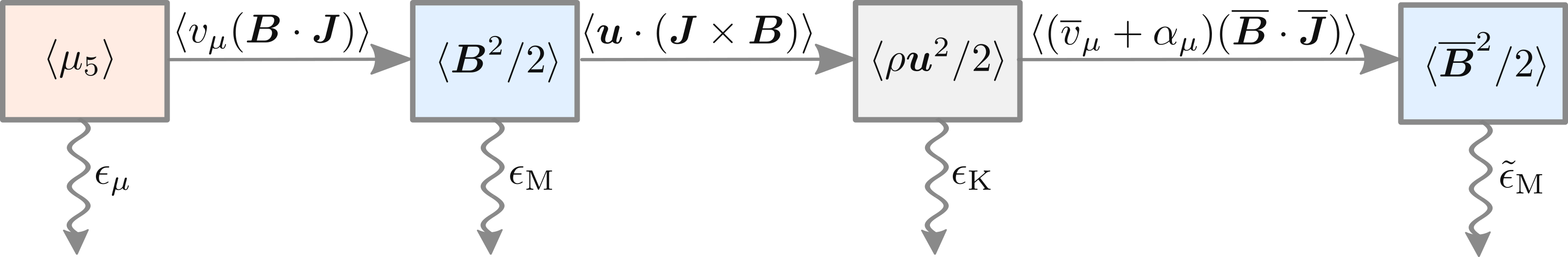
Figure 1: Illustration of energy transfer from the chiral chemical potential $\langle\mu_{5}\rangle$, to magnetic energy $\langle\bm{B}^{2}/2\rangle$, further to turbulent kinetic energy, $\langle\rho\bm{u}^{2}/2\rangle$ and finally to energy of the large-scale magnetic field, $\overline{\mbox{\boldmath$B$}}{}^{2}/2$. Losses via microscopic magnetic diffusion and kinematic viscosity are indicated by curled arrows. (colour online)

2.2 Analogy with the $\alpha$ effect in mean-field MHD

Readers familiar with mean-field MHD (see Moffatt, 1978; Krause and Rädler, 1980, mfMHD) will have readily noticed the analogy between $v_{\mu}=\mu\,\eta$ in chiral MHD and the kinetic part of the $\alpha$ effect, $\alpha_{\rm K}$, in mfMHD. For $\eta\to 0$, the analogy goes further in that even the evolution equation (6) for $\mu$ corresponds to an analogous one for the magnetic part of the $\alpha$ effect, $\alpha_{\rm M}$, proportional to the magnetic helicity, in what is known as the dynamical quenching formalism (Kleeorin and Ruzmaikin, 1982; Kleeorin et al., 1995).

Exploiting the analogy between chiral MHD and dynamical quenching can be beneficial in two ways. First, there is a considerable body of work on dynamical quenching that can improve our intuition in chiral MHD (e.g. Kleeorin et al., 2000; Blackman and Brandenburg, 2002). Second, numerical approaches have been developed for dynamical quenching that can directly be utilised in chiral MHD. The purpose of this section is to elaborate on this analogy, which was never mentioned before. Readers unfamiliar with dynamical quenching may skip forward to section 2.3.

In chiral MHD, dynamical quenching means that the total chirality, i.e., the sum of magnetic helicity and fermion chirality, is conserved. In mfMHD, in the absence of magnetic helicity fluxes, it implies that the total magnetic helicity is conserved, i.e., the sum of the magnetic helicity of the mean-field and that of the fluctuating field, the latter of which constitutes an additional time-dependent contribution to the $\alpha$ effect. The other contribution to the $\alpha$ effect in mfMHD, $\alpha_{\rm K}$, is proportional to the kinetic helicity, which was here assumed to be constant in time, so we can write (see equation 18 of Blackman and Brandenburg, 2002)

$$\frac{\partial\alpha}{\partial t}=\lambda_{\rm mfMHD}\,\eta\left[\eta_{{}_{T}}{\overline{\mbox{\boldmath$B$}}{}}{\bm\cdot}(\bm{\nabla}\times{\overline{\mbox{\boldmath$B$}}{}})-\alpha{\overline{\mbox{\boldmath$B$}}{}}^{2}\right]-{\varGamma}_{\rm mfMHD}\,(\alpha-\alpha_{\rm K}),$$ (10)

where $\alpha=\alpha_{\rm K}+\alpha_{\rm M}$. In mfMHD, the coupling coefficient is given by $\lambda_{\rm mfMHD}=2\eta_{{}_{T}}k_{\rm f}^{2}/(\eta B_{\rm eq}^{2})$ and ${\varGamma}_{\rm mfMHD}=2\eta k_{\rm f}^{2}$, where $k_{\rm f}$ is the wavenumber of the energy-carrying eddies and $B_{\rm eq}$ is the equipartition field strength.

The applications of chiral MHD carry over to decaying MHD turbulence with finite initial large-scale or small-scale magnetic helicity (Kemel et al., 2011). During the decay, some of the magnetic helicity is transferred between the large- and small-scale fields, which leads to a change in the $\alpha$ effect that in turn results in a slow-down of the decay.

2.3 Review of the three stages of the magnetic field evolution

Recent simulations by Schober et al. (2018) have demonstrated the existence of three distinct stages characterising the growth and saturation of the magnetic field in different kinds of chiral dynamos:
Phase 1: a laminar phase of small-scale chiral dynamo instability;
Phase 2: a large-scale dynamo instability, caused by chiral magnetically produced turbulence;
Phase 3: termination of growth of the large-scale magnetic field and reduction of $\mu$ according to the conservation law in chiral MHD.
With no further energy input, dynamo saturation is followed by decaying helical MHD turbulence, where the magnetic field decreases with time as a power law like $|\bm{B}|\sim t^{-1/3}$ (Biskamp and Müller, 1999; Kahniashvili et al., 2013).

In this section, the dynamics of chiral magnetically driven turbulence is shortly reviewed for the case of a chiral plasma in an infinite domain (see figure 2). In section 2.4, we will discuss the potential discrepancies in this picture arising from the effect of a finite computational domain (see figure 3).

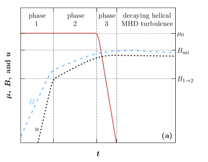
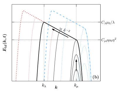
Figure 2: Schematic overview of the evolution of a plasma in an infinite box with an initially weak magnetic field in the presence of a chiral chemical potential. For a detailed discussion see section 2.3. (a): The time evolution of $\mu$ (red solid line), $\bm{u}$ (black dotted line), and $\bm{B}$ (blue dashed line). The values of $\mu_{0}$ and $B_{\mathrm{sat}}$ are indicated as horizontal dotted lines. The transitions between individual phases of the evolution are marked by vertical dashed-dotted lines. (b): Evolution of magnetic energy spectra with inverse transfer from $k_{\mu}$ to $k_{\lambda}$. The blue lines correspond to a larger $\mu_{0}$ in comparison with the case shown by the black lines (but for the same $\lambda$), while the red lines correspond to a smaller $\lambda$ in comparison with the case indicated by the black lines (but for the same $\mu_{0}$). (colour online)

2.3.1 Amplification of magnetic fields by chiral dynamos

In phase 1, the velocity field is negligible and a small-scale laminar dynamo operates. The growth rate found from the linearised equation (3) has a maximum value of (Joyce and Shaposhnikov, 1997)

$$\gamma_{\mu}=\frac{v_{\mu}^{2}}{4\eta}$$ (11)

being attained at

$$k_{\mu}=\frac{|\mu_{0}|}{2}.$$ (12)

While the magnetic field grows with a rate $\gamma_{\mu}$, turbulence is driven by the Lorentz force with the rms velocity increasing at a rate of approximately $2\gamma_{\mu}$.

In phase 2, the turbulent velocity has become so large that it affects the evolution of the magnetic field. It has been shown by Brandenburg et al. (2017b) that the peak of the magnetic energy spectrum reaches a value of

$$E_{\mathrm{M}}^{1\to 2}=C_{\mu}\overline{\rho}\mu_{0}\eta^{2}$$ (13)

with $C_{\mu}\approx 16$ at the transition from phase 1 to phase 2. This moment coincides with the beginning of the inverse transfer, when the $k^{-2}$ spectrum starts to build up, i.e. when the peak of the magnetic energy spectrum moves from $k_{\mu}$ to smaller wavenumbers. The corresponding transition field strength can be estimated as

$$B_{\mathrm{rms}}^{1\to 2}\approx\left(E_{\mathrm{M}}^{1\to 2}k_{\mu}\right)^{1/2}\approx\left(\frac{C_{\mu}\overline{\rho}}{2}\right)^{1/2}\mu_{0}\eta.$$ (14)

At this stage, the chiral magnetically produced turbulence causes excitation of a large-scale magnetic field by the chiral $\alpha_{\mu}$ effect. This chiral large-scale dynamo, studied by Rogachevskii et al. (2017), occurs at the maximum growth rate

$$\gamma_{\alpha}={(\overline{v}_{\mu}+\alpha_{\mu})^{2}\over 4(\eta+\,\eta_{{}_{T}})}={(\overline{v}_{\mu}+\alpha_{\mu})^{2}\over 4\eta\,(1+\,{\rm Re}_{{}_{\mathrm{M}}}/3)},$$ (15)

where $\overline{v}_{\mu}\equiv\eta\overline{\mu}$ and $\overline{\mu}$ is the mean chiral chemical potential. Despite the contribution from the chiral $\alpha_{\mu}$ effect, given by the term $\alpha_{\mu}=-{2\over 3}\overline{v}_{\mu}\ln{\rm Re}_{{}_{\mathrm{M}}}$, the overall growth rate is reduced as compared to the laminar chiral dynamo. Here, ${\rm Re}_{{}_{\mathrm{M}}}$ is the magnetic Reynolds number defined by ${\rm Re}_{{}_{\mathrm{M}}}=u_{\mathrm{rms}}/(\eta k_{\mathrm{f}})=3\eta_{{}_{T}}/\eta$ The maximum growth rate of the chiral large-scale dynamo is attained at the wavenumber $k_{\alpha}=|\overline{v}_{\mu}+\alpha_{\mu}|/(2\eta+\,2\eta_{{}_{T}})$.

2.3.2 Saturation of the chiral large-scale dynamo

Saturation of the chiral large-scale dynamo, phase 3, is controlled by the conservation law following from equations (3)–(6), which implies that the total chirality

$$\frac{\lambda}{2}\overline{\mbox{\boldmath$A\cdot B$}}{}+\bar{\mu}=\mu_{0}=\mathrm{const},$$ (16)

is a conserved quantity; see Rogachevskii et al. (2017) for more details. Here, $\overline{\mbox{\boldmath$A\cdot B$}}{}$ is the spatially averaged value of the magnetic helicity. According to the conservation law (16), the magnetic field reaches $B_{\mathrm{sat}}=\left(\mu_{0}/(\lambda\xi_{\mathrm{M}})\right)^{1/2}$, where $\xi_{\mathrm{M}}$ is the correlation length of the magnetic field.

The magnetic energy spectrum $E_{\rm M}(k,t)$ in chiral MHD turbulence has been studied in Brandenburg et al. (2017b). In particular, it was found that $E_{\rm M}$ is proportional to $k^{-2}$ between the wavenumber

$$k_{\lambda}=\sqrt{\overline{\rho}\lambda\frac{C_{\mu}}{C_{\lambda}}}\,\eta\mu_{0},$$ (17)

with $C_{\mu}\approx 16$, $C_{\lambda}\approx 1$, and $k_{\mu}$ given by equation (12). We note that the only case considered here is $\lambda_{\mu}\ll 1$, which implies $k_{\lambda}\ll k_{\mu}$. Using dimensional arguments and numerical simulations, Brandenburg et al. (2017b) found that for chiral magnetically driven turbulence, the saturation magnetic energy spectrum $E_{\rm M}(k,t)$ obeys

$$E_{\rm M}(k,t)=C_{\mu}\,\overline{\rho}\mu_{0}^{3}\eta^{2}k^{-2}$$ (18)

in $k_{\lambda}<k<\mu_{0}$. Here, $E_{\rm M}(k,t)$ is normalised such that the mean magnetic energy density is $\langle\bm{B}^{2}\rangle/2=\int E_{\rm M}(k)\,\mathrm{d}k$. It was also confirmed numerically by Brandenburg et al. (2017b) that the magnetic energy spectrum $E_{\rm M}(k)$ is limited from above by $C_{\lambda}\mu_{0}/\lambda$. The magnetic field strength at dynamo saturation can be estimated as

$$B_{\mathrm{sat}}\approx\left(E_{\rm M}(k_{\lambda})k_{\lambda}\right)^{1/2}=\left(\frac{\overline{\rho}\eta^{2}C_{\mu}C_{\lambda}}{\lambda}\right)^{1/4}\mu_{0}.$$ (19)

In figure 2(a) the effect of changing $\mu_{0}$ and $\lambda$ on the final energy spectrum is illustrated. Here, intermediate spectra are shown as thin lines, while thick lines indicate the magnetic energy spectrum at saturation with an inertial range where $E_{\mathrm{M}}\propto k^{-2}$ between $k_{\lambda}$ and $k_{\mu}$. The black lines present a case with a certain $\mu_{\mathrm{black}}$ and $\lambda_{\mathrm{black}}$. If $\lambda$ is decreased, $k_{\lambda}$ also decreases, and the $k^{-2}$ spectrum spans over a larger range of wavenumbers. This is illustrated by the red lines, where $\mu_{\mathrm{red}}=\mu_{\mathrm{black}}$ and $\lambda_{\mathrm{red}}<\lambda_{\mathrm{black}}$. In this case, the final magnetic field strength is higher than in the case with $\mu_{\mathrm{black}}$ and $\lambda_{\mathrm{black}}$. The same final field strength can, however, also be reached by increasing $\mu_{0}$, as $B_{\mathrm{sat}}\propto\mu_{0}/\lambda^{1/4}$. Schematic spectra illustrating the latter case are shown as blue curves in figure 2, where $\mu_{\mathrm{blue}}>\mu_{\mathrm{black}}$ and $\lambda_{\mathrm{blue}}=\lambda_{\mathrm{black}}$.

2.4 Effects of the finite numerical domain

Due to a finite simulation domain, the evolution of the magnetic field and the turbulent velocity is slightly modified in comparison to the case discussed in section 2.3. The evolution of the chiral chemical potential, the magnetic field strength, the rms velocity, and the time evolution of the magnetic energy spectra in finite box simulations are illustrated in figure 3.

First of all, the chiral chemical potential, does not vanish at dynamo saturation, but reaches a finite value, which is equal to the minimum wavenumber possible in the box, $k_{1}$. The magnetic field reaches the saturation value given by equation (19). However, the evolution of the magnetic energy spectrum differs compared to that anticipated for an infinite system. In the laminar chiral dynamo phase, we expect an instability at wavenumber $k_{\mu}$, as predicted by theory; see the black curves in figure 3(b). With the production of turbulence, the peak of the magnetic energy spectrum moves to larger spatial scales through inverse transfer. As discussed above, we expect a scaling of the magnetic energy spectrum proportional to $k^{-2}$; see equation (18). Once the peak reaches the size of the box, however, we observe a steepening of the spectrum, as indicated in the schematic figure 3, if $k_{\lambda}<k_{1}$. This steepening is caused by the growth of the magnetic field on the smallest possible wavenumber, until the spectrum reaches its saturation value $C_{\lambda}\mu_{0}/\lambda$. For large values of $\mu_{0}$, the initial chiral dynamo instability occurs at smaller spatial scales, i.e., at larger wavenumbers $k$, and thus the $k^{-2}$ spectrum can extend over a larger range; see the blue curves in figure 3(b). In this paper, we present also a run with $k_{\lambda}\approx k_{1}$, run B, which has a resolution of $1216^{3}$. Large parameter scans, and cases with larger scale separation, $k_{\lambda}\gg k_{1}$, are computationally too expensive.

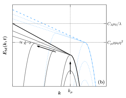
Figure 3: Same as figure 2 but including effects of a finite box. (colour online)

3 Chiral magnetically driven turbulence in direct numerical simulations

3.1 Numerical setup

We solve equations (3)–(6) in a three-dimensional periodic domain of size $L^{3}=(2\pi)^{3}$ with the Pencil Code. This code is well suited for MHD studies; it employs a third-order accurate time-stepping method of Williamson (1980) and sixth-order explicit finite differences in space (Brandenburg and Dobler, 2002; Brandenburg, 2003). The smallest wavenumber covered in the numerical domain is $k_{1}=2\pi/L=1$ and the resolution is varied between $480^{3}$ and $1216^{3}$. For comparison, we also show some simulations that have previously been presented (Schober et al., 2018), but we now include additional runs for ${\rm Pr}_{{}_{\mathrm{M}}}\neq 1$. The sound speed in the simulations is set to $c_{\rm s}=1$ and the mean fluid density to $\overline{\rho}=1$. If not indicated otherwise, the magnetic Prandtl number is $1$, i.e. the magnetic diffusivity equals the viscosity. However, we do consider cases between ${\rm Pr}_{{}_{\mathrm{M}}}=0.5$ and ${\rm Pr}_{{}_{\mathrm{M}}}=10$, where the value of $\eta$ is fixed and $\nu$ changes. No external forcing is applied to drive turbulence in these simulations, i.e., the velocity field is then driven entirely by magnetic fields. All runs are initialised with a weak seed magnetic field in the form of Gaussian noise, with constant $\mu$, and vanishing velocity. The main input parameters of all simulations presented in this paper are summarised in table 2.

Table 2: Overview of the input parameters of all simulations discussed in this paper. We list the values of the non-dimensional chiral parameters, ${\rm Ma}_{\mu}$ and $\lambda_{\mu}$, see equations (8) and (9), respectively, as well as the characteristic wavenumbers, $k_{\mu}$ and $k_{\lambda}$, see equations (12) and (17), normalized by the minimum wavenumber corresponding to the finite numerical domain, $k_{1}$. Runs D, F, G and H have been performed with different magnetic Prandtl numbers, i.e., run D05 with ${\rm Pr}_{{}_{\mathrm{M}}}=0.5$, run D1 with ${\rm Pr}_{{}_{\mathrm{M}}}=1$, up to run D10 with ${\rm Pr}_{{}_{\mathrm{M}}}=10$. Reference runs are highlighted by bold font.

simulation	resolution	${\rm Ma}_{\mu}$	$\lambda_{\mu}$	$(\mu_{0}/\lambda)^{1/2}$	$k_{\mu}/k_{1}$	$k_{\lambda}/k_{1}$	${\rm Pr}_{{}_{\mathrm{M}}}$
Run A	$\mathbf{576^{3}}$	$\mathbf{2\times 10^{-3}}$	$\mathbf{2\times 10^{-7}}$	$\mathbf{1.00}$	$\mathbf{10}$	$\mathbf{0.036}$	$\mathbf{1.0}$
Run B	$1216^{3}$	$6.6\times 10^{-3}$	$9\times 10^{-6}$	$0.12$	$44$	$1.1$	$1.0$
Run C	$480^{3}$	$1.5\times 10^{-3}$	$5\times 10^{-6}$	$0.12$	$15$	$0.27$	$1.0$
Runs D05…10	$\mathbf{480^{3}}$	$\mathbf{2\times 10^{-3}}$	$\mathbf{5\times 10^{-6}}$	$\mathbf{0.14}$	$\mathbf{20}$	$\mathbf{0.36}$	$\mathbf{0.5...10}$
Run E	$480^{3}$	$2.5\times 10^{-3}$	$5\times 10^{-6}$	$0.16$	$25$	$0.45$	$1.0$
Runs F1…10	$576^{3}$	$3\times 10^{-3}$	$5\times 10^{-6}$	$0.17$	$30$	$0.54$	$0.5...10$
Runs G05…10	$480^{3}$	$4\times 10^{-3}$	$2\times 10^{-5}$	$0.14$	$20$	$0.72$	$0.5...10$
Runs H05…10	$480^{3}$	$8\times 10^{-3}$	$2\times 10^{-5}$	$0.28$	$20$	$0.72$	$0.5...10$

3.2 Reference run for chiral magnetically driven turbulence

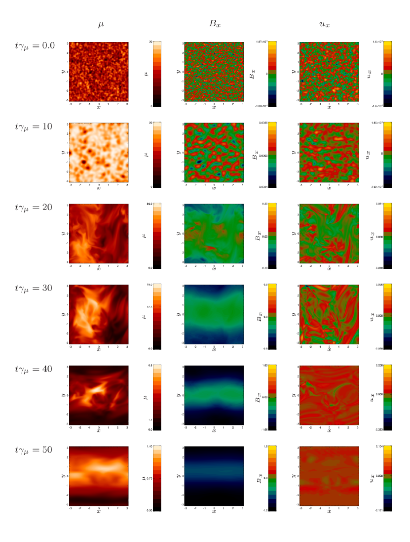
Figure 4: Cross sections of the chiral chemical potential ($\mu$, left column), as well as the $x$ components of the magnetic field ($B_{x}$, middle column), and the velocity field ($u_{x}$, right column) in the $xy$ plane. From top to bottom the time increases from $0$ to $50~{}\gamma_{\mu}^{-1}$, during which the chiral MHD dynamo generates a large-scale magnetic field and a velocity field.

The generation of the magnetic field by the laminar chiral dynamo, and after that by the chiral mean-field dynamo, can be seen in figure 4, where we present snapshots of $\mu$ (left column), $B_{x}$ (middle column), and $u_{x}$ (right column) for run A. As indicated on the left, from top to bottom the time increases from $t=0$ to $t\gamma_{\mu}=50$. In the following, we summarise the quantitative analysis of run A, but we refer to section 4 of Schober et al. (2018) for a more detailed discussion of this simulation.

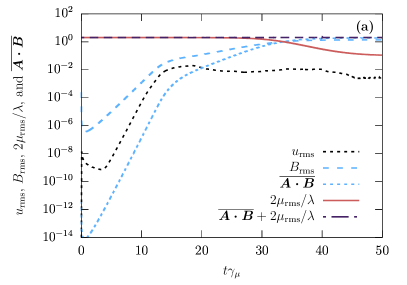
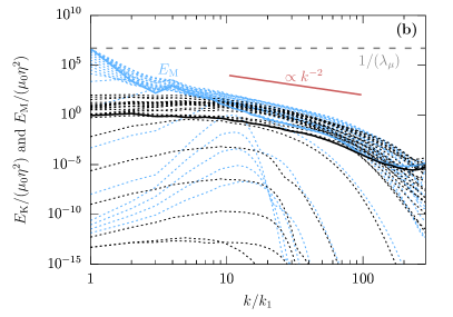
Figure 5: (a) The time evolution of the most relevant parameters in the reference run A. This run has been discussed in greater detail in section 4 of Schober et al. (2018), where this plot is shown in the top panel of their figure 9. (b) Normalized energy and helicity spectra for the reference run A. The time intervals between two spectra are equidistant and the last spectra are presented by solid lines. This plot is equivalent to figure 10 of Schober et al. (2018). (colour online)

The time evolution of the key quantities for the reference run A is shown in figure 5. As can be seen in figure 5(a), $B_{\mathrm{rms}}$ (blue dashed line) increases exponentially by over $4$ orders of magnitude before the growth rate decreases due to the produced turbulence. Saturation of the magnetic field growth occurs at $t\gamma_{\mu}\approx 40$. Both, the velocity $u_{\mathrm{rms}}$ (black dotted line) and the magnetic helicity $\overline{\mbox{\boldmath$A\cdot B$}}{}$ (blue dotted line) increase at a rate twice the one of $B_{\mathrm{rms}}$. The value of $\mu_{\mathrm{rms}}$ (orange solid line), here shown with a constant factor $2/\lambda$, decreases only above $t\gamma_{\mu}\approx 30$, switching off the chiral dynamo instability. In accordance with the conservation law (16), the sum $\overline{\mbox{\boldmath$A\cdot B$}}{}+2\mu_{\mathrm{rms}}/\lambda$ (purple dashed-dotted line) is constant throughout the simulation time.

In figure 5(b), the evolution of the magnetic (blue lines) and kinetic (black lines) energy spectra for run A are presented. It can be seen that the laminar chiral dynamo injects energy at the wavenumber $k_{\mu}$, as given in equation (12). Once turbulence has been produced, the magnetic correlation length moves to smaller wavenumbers due to mode coupling, similarly to what has been seen previously in dynamos driven by the Bell instability (Rogachevskii et al., 2012). Eventually, the energy accumulates on $k=k_{1}$; see the final spectra in the simulation which are plotted with solid lines.

3.3 Turbulence in different scenarios

In chiral MHD, energy is transformed from the chiral chemical potential, to magnetic energy, and later to turbulent kinetic energy; see figure 1. For a quantification of this energy transfer, it is useful to compare the production rate of turbulent kinetic energy, $\langle\bm{U}\cdot(\bm{J}\times\bm{B})\rangle$, with the one of the magnetic field, $|v_{\mu}\bm{B}\cdot\nabla\times\bm{B}|$. Therefore, we define the dimensionless ratio

$${\varPhi}\equiv\frac{\langle\bm{U}\cdot(\bm{J}\times\bm{B})\rangle}{|v_{\mu}\bm{B}\cdot\nabla\times\bm{B}|},$$ (20)

where we have assumed that $\bm{B}\cdot\nabla\times\bm{B}\approx k_{\mathrm{M}}B_{\mathrm{rms}}^{2}$ with the inverse magnetic correlation length, $k_{\mathrm{M}}^{-1}$.

Furthermore, it is useful to determine the value of turbulent kinetic energy that can be produced in chiral MHD without external forcing of turbulence. In the analysis of run A, we have seen that the kinetic energy reaches a certain percentage of the magnetic energy. With the onset of the large-scale dynamo phase, phase 2, the ratio

$${\varUpsilon}\equiv\frac{\rho u_{\mathrm{rms}}^{2}/2}{B_{\mathrm{rms}}^{2}/2}$$ (21)

stays approximately constant and decreases as soon as the peak of the magnetic energy spectrum reaches the box wavenumber $k_{1}$. Afterwards, turbulence is not driven by the Lorentz force anymore and the velocity field decays.

In this section, we explore how the details of this scenario are affected by the properties of the plasma. In particular, we perform a parameter scan, varying the chiral parameters as well as the magnetic Prandtl number.

3.3.1 Dependence on the chiral parameters $\mathrm{Ma}_{\mu}$ and $\lambda_{\mu}$

The time evolution of the ratio ${\varUpsilon}$ is presented in figure 6(a) for runs with different values of $\mathrm{Ma}_{\mu}$ and $\lambda_{\mu}$. Time is normalised here by the inverse of the laminar dynamo growth rate (11), allowing comparison between runs with different $v_{\mu}$. The evolution of ${\varUpsilon}$ in all runs is similar up to $t\approx 12\,\gamma_{\mu}^{-1}$, except for a minor time delay of run A. This can be explained by the effect of magnetic diffusivity which is larger than the one in run C by a factor of two. Phase 2, when turbulence affects the evolution of the magnetic field, begins approximately at $t\approx(12$–$14)~{}\gamma_{\mu}^{-1}$ for the runs considered here. The onset of phase 2 is weakly dependent on $\eta$ and, in principle, also on the initial value of the magnetic field strength, which is the same for all runs presented in this paper. During phase 2, the ratio ${\varUpsilon}$ is comparable for all three runs considered here, even though $\mathrm{Ma}_{\mu}$ and $\lambda_{\mu}$ are different. Once the chiral large-scale dynamo phase begins, we obtain the ratio ${\varUpsilon}\lesssim 0.1$.

Run A, the reference run discussed in the previous section, has the lowest value of $\lambda$ in our sample, leading to a small value of $k_{\lambda}$ in comparison to the maximum wavenumber in the box: $k_{\lambda}\approx 0.036k_{1}$. This implies that $k_{1}$ is reached early, much before dynamo saturation, and the kinetic energy decays. As long as $k_{\mathrm{M}}>k_{1}$, a solid line style is used in figure 6, while for late times, the time evolution is presented with dashed lines to indicate the finite box effect. Here, $k_{\mathrm{M}}$ has been determined as the peak of the energy spectra. To observe a scenario in which the complete inverse cascade takes place inside the box, so that the kinetic energy does not decay within phase 2, we have performed run B. The choice of the parameters for this run, listed in table 2, can be justified as follows: As for all of the runs presented in this paper, the ratio between $k_{\mu}$ and $k_{\lambda}$ needs to be large, in order to observe a chiral large-scale dynamo phase (phase 2). Using equations (12) and (17), we see that

$$\frac{k_{\mu}}{k_{\lambda}}=\left(\frac{C_{\lambda}}{4C_{\mu}}\frac{1}{\overline{\rho}\eta^{2}\lambda}\right)^{1/2}=\left(\frac{C_{\lambda}}{4C_{\mu}}\frac{1}{\lambda_{\mu}}\right)^{1/2},$$ (22)

which is independent of $\mu_{0}$. However, $\mu_{0}$ needs to be chosen high enough to ensure that $k_{\lambda}>k_{1}$. In run B, we use $\mu_{0}/k_{1}=88$, which implies that the laminar dynamo instability occurs on small spatial scales and a high numerical resolution is required. Run B is presented in figure 6(a) as a grey solid line, for which the ratio ${\varUpsilon}$ remains approximately constant for times larger than $\approx 12~{}\gamma_{\mu}^{-1}$.

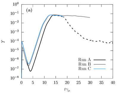
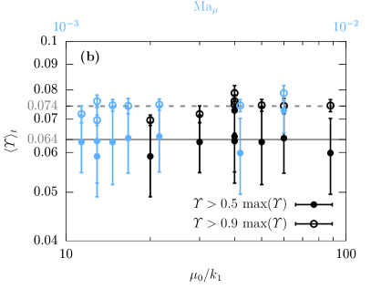
Figure 6: (a) The ratio of kinetic over magnetic energy, ${\varUpsilon}$, as a function of time, normalized by $\gamma_{\mu}^{-1}$, for runs A–C; see table 2. The time during which $k_{\mathrm{M}}$ is inside the numerical box, i.e., $k_{\mathrm{M}}>k_{1}$, is marked by solid line style. For $k_{\mathrm{M}}<k_{1}$, the lines are dashed. (b) The time averaged ratio ${\varPhi}$ as a function of $\mu_{0}/k_{1}$ (lower abscissa, black symbols) and a function of $\mathrm{Ma}_{\mu}$ (upper abscissa, blue symbols) for all runs with ${\rm Pr}_{{}_{\mathrm{M}}}=1$. For the results shown as filled dots, the average has been performed for the time interval for which ${\varUpsilon}$ is at least 50% of its maximum value. For open dots, the time average is taken for all ${\varUpsilon}>0.9~{}\mathrm{max}({\varUpsilon})$. The solid grey line shows the mean value of $\langle\varUpsilon\rangle_{t}$ resulting from the first time averaging condition and the dashed grey for the latter condition. (colour online)

In figure 6(b), we show the time averaged ratio $\langle\varUpsilon\rangle_{t}$ for all our runs with ${\rm Pr}_{{}_{\mathrm{M}}}=1$ as a function of $\mu_{0}/k_{1}$ as black symbols. The blue symbols refer to the upper $x$ axes and indicate the corresponding value of $\mathrm{Ma}_{\mu}$. For the time averaging procedure, we consider two different criteria: For solid symbols the time average is performed for all values of ${\varUpsilon}$ larger than 50% of its maximum value. The open dots are obtained by using all values for which ${\varUpsilon}>0.9~{}\mathrm{max}({\varUpsilon})$, which obviously results in a larger average value. Error bars represent the standard deviation of $\langle\varUpsilon\rangle_{t}$. There is no significant dependence of $\langle\varUpsilon\rangle_{t}$ on the values of $\mu_{0}$ and $\mathrm{Ma}_{\mu}$ for the parameter space explored here: When averaging over all ${\varUpsilon}>0.5~{}\mathrm{max}({\varUpsilon})$, we find a mean $\langle\varUpsilon\rangle_{t}\approx 0.064$, and when employing the criterion ${\varUpsilon}>0.9~{}\mathrm{max}({\varUpsilon})$, we find $\langle\varUpsilon\rangle_{t}\approx 0.074$.

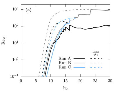
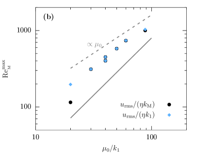
Figure 7: (a) The magnetic Reynolds number ${\rm Re}_{{}_{\mathrm{M}}}$ as a function of time for runs A–C. The solid lines indicate the result using $k_{\mathrm{M}}$ as the integral scale of turbulence and dashed lines show the result using $k_{1}$. At late times $k_{\mathrm{M}}=k_{1}$ in our DNS, which are confined within a finite box. (b) The maximum magnetic Reynolds number found in our simulations versus $\mu_{0}/k_{1}$, for both cases ${\rm Re}_{{}_{\mathrm{M}}}=u_{\mathrm{rms}}/(\eta k_{1})$ (black dots) and ${\rm Re}_{{}_{\mathrm{M}}}=u_{\mathrm{rms}}/(\eta k_{\mathrm{M}})$ (blue diamonds). The solid line indicates the scaling $\mu_{0}^{3/2}$ which is expected for finite box simulations with $k_{1}>k_{\lambda}$. (colour online)

To estimate the magnetic Reynolds number, we need to determine the amount of turbulent kinetic energy that can be produced by the Lorentz force. The value of ${\rm Re}_{{}_{\mathrm{M}}}$ is determined by the rms velocity, the magnetic diffusivity, and the correlation length of the magnetic field, $k_{\mathrm{M}}^{-1}$. In numerical simulations, both $u_{\mathrm{rms}}$ and $k_{\mathrm{M}}$ can be limited by the size of the box, while $\eta$ is an input parameter. We have seen that $\langle\varUpsilon\rangle_{t}$ has an approximately fixed value in the mean-field dynamo phase for ${\rm Pr}_{{}_{\mathrm{M}}}=1$ and as long as $k_{\mathrm{M}}>k_{1}$. This implies that the value of $u_{\mathrm{rms}}$ is proportional to $B_{\mathrm{rms}}$ and reaches a maximum at the time $t_{\mathrm{box}}$, which is defined as the time when the peak of the energy spectrum reaches the size of the box, i.e., when $k_{\mathrm{M}}=k_{1}$. The energy spectrum at this time, described by equation (18), reaches a maximum $E_{\mathrm{M}}(k_{1},t_{\mathrm{box}})=C_{\mu}\overline{\rho}\eta^{2}\mu_{0}^{3}/2$. The magnetic field strength corresponding to this energy spectrum can be estimated as $[E_{\mathrm{M}}(k_{1},t_{\mathrm{box}})k_{1}]^{1/2}=(C_{\mu}\overline{\rho}/2)^{1/2}\eta\mu_{0}^{3/2}$. Hence we expect a scaling of the maximum velocity in our simulations $\propto\eta\mu_{0}^{3/2}$. The magnetic Reynolds number, ${\rm Re}_{{}_{\mathrm{M}}}=u_{\mathrm{rms}}/(\eta k_{\mathrm{M}})$ with $k_{\mathrm{M}}=k_{1}$ at late times, is thus independent of $\eta$ and scales as $\mu_{0}^{3/2}$. This scaling is observed in our simulations; see figure 7(b). The Reynolds number as a function of time for runs with different $\mu_{0}/k_{1}$ is presented in figure 7(a). Here, we show two different ratios, $u_{\mathrm{rms}}/(\eta k_{\mathrm{M}})$ and $u_{\mathrm{rms}}/(\eta k_{1})$. For the first case, $k_{\mathrm{M}}$ is measured as a function of time using the magnetic energy spectra. At late times, once the peak of the magnetic energy spectrum has reached the box wavenumber, $k_{\mathrm{M}}=k_{1}$, and the dashed and solid curves for individual runs coincide.

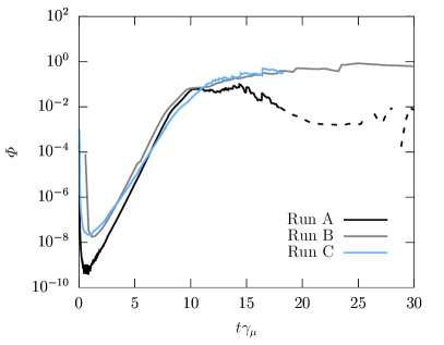
Figure 8: Same as figure 6(a), but for the ratio of the production rate of kinetic energy over the production rate of magnetic energy, ${\varPhi}$. (colour online)

The ratio of the production rate of kinetic energy over the production rate of magnetic energy, ${\varPhi}$, is presented in figure 8. For runs A, B, C, it can be seen how ${\varPhi}$ increases exponentially with a rate $\approx 2\gamma_{\mu}$ like the velocity field. In phase 2, the growth rate decreases, and ${\varPhi}$ seems to converge to a value of $\approx 1$ at dynamo saturation, implying that the transfer rate from the chiral chemical potential to magnetic energy and the transfer rate from magnetic energy to kinetic energy become comparable. Again, run A differs from runs B and C, due to the fact that the magnetic correlation length reaches the size of the domain at $t\gamma_{\mu}\approx 17$, which is well before dynamo saturation. In order to perform a quantitative analysis of the dependence of ${\varPhi}$ on the plasma parameters, it would be necessary to run the numerical simulations for a much longer time, i.e., until dynamo saturation, and to increase the size of the simulation domain to ensure $k_{1}<k_{\mathrm{M}}$. This is, however, too expensive and beyond the scope of this paper.

3.3.2 Dependence on the magnetic Prandtl number

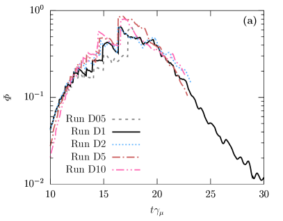
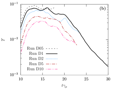
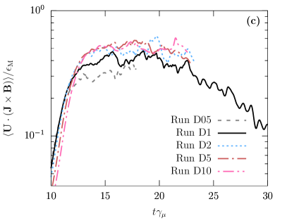
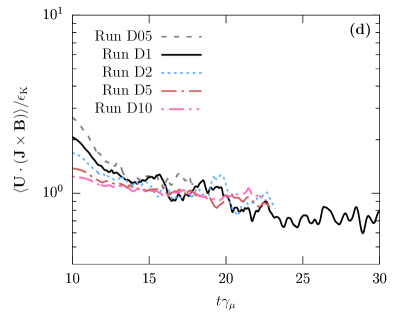
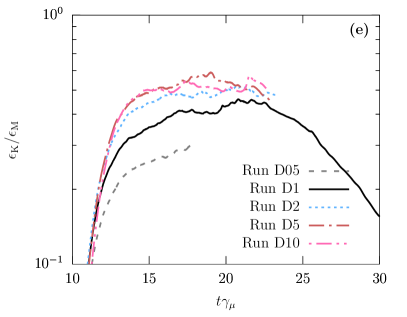
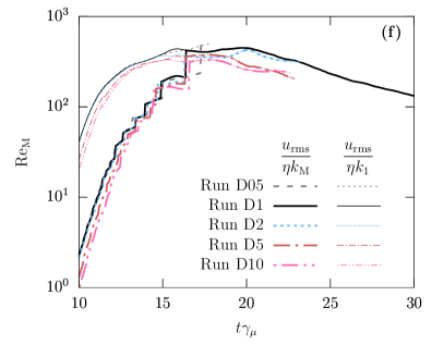
Figure 9: Time series of the ratio of (a) energy transfer rates ${\varPhi}$, (b) the energy ratio ${\varUpsilon}$, (c) $\langle\bm{U}\cdot(\bm{J}\times\bm{B})\rangle/\epsilon_{\mathrm{M}}$, (d) $\langle\bm{U}\cdot(\bm{J}\times\bm{B})\rangle/\epsilon_{\mathrm{K}}$, (e) $\epsilon_{\mathrm{K}}/\epsilon_{\mathrm{M}}$, and (f) ${\rm Re}_{{}_{\mathrm{M}}}$ for series D; see table 2. (colour online)

We have performed a series of runs with different magnetic Prandtl numbers by changing the value of $\nu$, in order to explore trends in the conversion of magnetic to kinetic energy. The time series of the most relevant quantities are discussed here exemplary for the runs of series D, where ${\rm Pr}_{{}_{\mathrm{M}}}$ varies between $0.5$ and $10$ while all other run parameters are unchanged; see table 2. It should be noted that low ${\rm Pr}_{{}_{\mathrm{M}}}$ are difficult to obtain in DNS at fixed $\eta$, as an increase of resolution is required when decreasing $\nu$, making a quantitative study of the low Prandtl number regime inaccessible to our current simulations.

In figure 9(a), ${\varPhi}$ is presented as a function of time. It should be noted, that the magnetic correlation length reaches $k_{1}^{-1}$ at a time of $t\gamma_{\mu}\approx 20$. Later times should not be discussed due to numerical artefacts discussed before. Up to $t\gamma_{\mu}\approx 20$, we do not observe a significant ${\rm Pr}_{{}_{\mathrm{M}}}$-dependence of ${\varPhi}$. The ratio ${\varUpsilon}$, presented in figure 10(b), on the other hand decreases significantly with increasing ${\rm Pr}_{{}_{\mathrm{M}}}$.

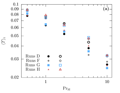
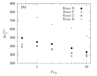
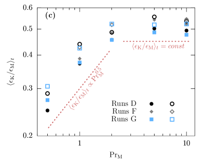
Figure 10: (a) The time averaged value of ${\varUpsilon}$ for different run series. Filled symbols represent the result from an time averaging of all data points with ${\varUpsilon}>0.5~{}\mathrm{max}({\varUpsilon})$ and open symbols averaging is performed for all data with ${\varUpsilon}>0.9~{}\mathrm{max}({\varUpsilon})$. Errors are of the the order of 10% for the filled symbols and 5% for the open symbols, but not presented in the figure for better visualization. (b) The maximum magnetic Reynolds number in the different DNS as a function of ${\rm Pr}_{{}_{\mathrm{M}}}$. (c) The time averaged ratio of viscous over Joule dissipation, $\langle\epsilon_{\mathrm{K}}/\epsilon_{\mathrm{M}}\rangle_{t}$, as a function of ${\rm Pr}_{{}_{\mathrm{M}}}$. Again, for filled symbols, the average of $\epsilon_{\mathrm{K}}/\epsilon_{\mathrm{M}}$ is calculated for all values $\epsilon_{\mathrm{K}}/\epsilon_{\mathrm{M}}>0.5~{}\mathrm{max}(\epsilon_{\mathrm{K}}/\epsilon_{\mathrm{M}})$ and for open symbols, averaging is performed for $\epsilon_{\mathrm{K}}/\epsilon_{\mathrm{M}}>0.9~{}\mathrm{max}(\epsilon_{\mathrm{K}}/\epsilon_{\mathrm{M}})$. (colour online)

In the middle panels (c),(d) of figure 9, we present the time evolution of additional characteristics describing the transfer from kinetic to magnetic energy. We find that both, the work done by the Lorentz force, $\langle\mathbf{U}\cdot(\mathbf{J}\times\mathbf{B})\rangle$, and the ratio of viscous over Joule dissipation, $\epsilon_{\mathrm{K}}/\epsilon_{\mathrm{M}}$ depend on ${\rm Pr}_{{}_{\mathrm{M}}}$. The latter dissipation ratio is expected to increase with ${\rm Pr}_{{}_{\mathrm{M}}}$ for large-scale and small-scale dynamos in classical MHD; see Brandenburg (2014). This trend of $\epsilon_{\mathrm{K}}/\epsilon_{\mathrm{M}}$ with ${\rm Pr}_{{}_{\mathrm{M}}}$ is also observed in our DNS of chiral large-scale dynamos; see also figure 10(c). However, we do observe a power-law scaling of $\langle\epsilon_{\mathrm{K}}/\epsilon_{\mathrm{M}}\rangle_{t}$ with ${\rm Pr}_{{}_{\mathrm{M}}}$ only below ${\rm Pr}_{{}_{\mathrm{M}}}\approx 2$. For larger Prandtl numbers the ratio becomes constant.

The maximum magnetic Reynolds numbers, ${\rm Re}_{{}_{\mathrm{M}}}^{\mathrm{max}}$, obtained in series D, are presented figure 10(b). It can be seen that a dependence of ${\rm Re}_{{}_{\mathrm{M}}}^{\mathrm{max}}$ on ${\rm Pr}_{{}_{\mathrm{M}}}$ is caused by the decrease of $u_{\mathrm{rms}}$ with increasing ${\rm Pr}_{{}_{\mathrm{M}}}$. As discussed in the previous section, a change of ${\rm Re}_{{}_{\mathrm{M}}}$ in DNS with $k_{\lambda}<k_{1}$ can only be achieved by changing $\mu_{0}$.

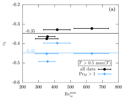
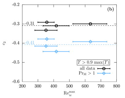
Figure 11: The slope resulting from a fit of the function $\langle\varUpsilon\rangle_{t}=c_{1}{\rm Pr}_{{}_{\mathrm{M}}}^{c_{2}}$ to the data points presented in figure 10(a) as a function of the range of maximum magnetic Reynolds numbers found in simulations shown in figure 10(b). The horizontal bars indicate the range of ${\rm Re}_{{}_{\mathrm{M}}}^{\mathrm{max}}$, which decreases from small to large ${\rm Pr}_{{}_{\mathrm{M}}}$. Results for the fitting to all data are shown as black symbols and results for using ${\rm Pr}_{{}_{\mathrm{M}}}>1$ as blue diamonds. Horizontal lines indicate the average values of the slopes. (a) $\langle\varUpsilon\rangle_{t}$ has been obtained using all data with ${\varUpsilon}>0.5~{}\mathrm{max}({\varUpsilon})$. (b) $\langle\varUpsilon\rangle_{t}$ has been obtained using all data with ${\varUpsilon}>0.9~{}\mathrm{max}({\varUpsilon})$. (colour online)

We now check if a power-law fit, $\langle\varUpsilon\rangle_{t}=c_{1}{\rm Pr}_{{}_{\mathrm{M}}}^{c_{2}}$, is consistent with the data of the fit parameters $c_{1}$ and $c_{2}$. Both averaging conditions, using all data points for which ${\varUpsilon}>0.5~{}\mathrm{max}({\varUpsilon})$ and ${\varUpsilon}>0.9~{}\mathrm{max}({\varUpsilon})$, are considered. The results for the full range of ${\rm Pr}_{{}_{\mathrm{M}}}$ as well as for ${\rm Pr}_{{}_{\mathrm{M}}}>1$ can be found in the appendix in table 3. Additionally, we present the slopes $c_{2}$ as a function of the corresponding range of $\mathrm{Re}_{\mathrm{M,max}}$ in figure 11. Fit results to the ${\varUpsilon}>0.5~{}\mathrm{max}({\varUpsilon})$ condition are shown in figure 11(a) and the case of ${\varUpsilon}>0.9~{}\mathrm{max}({\varUpsilon})$ in figure 11(b). The obtained value of $c_{2}$ is presented for fitting to all available data as black symbols and for ${\rm Pr}_{{}_{\mathrm{M}}}>1$ as blue ones. We do not find a clear dependence of $c_{2}$ on the Reynolds number range. When using data for the full ${\rm Pr}_{{}_{\mathrm{M}}}$ regime explored in this paper, we find mean slopes between $c_{2}=-0.31$ and $-0.35$. The slope of the function $\langle\varUpsilon\rangle_{t}({\rm Pr}_{{}_{\mathrm{M}}})$ becomes steeper with values between $c_{2}=-0.41$ and $c_{2}=-0.45$, when fitting only to data with ${\rm Pr}_{{}_{\mathrm{M}}}>1$. The latter should be a better description for the large Prandtl number regime, since the scaling of $\langle\varUpsilon\rangle_{t}$ might change in the transition from ${\rm Pr}_{{}_{\mathrm{M}}}<1$ to ${\rm Pr}_{{}_{\mathrm{M}}}>1$.

4 Chiral magnetically driven turbulence in the early Universe

The findings from DNS presented above can be leveraged to estimate the turbulent velocities and the Reynolds number in the early Universe. As we have seen in the previous section, the ratio of kinetic to magnetic energy depends on the magnetic Prandtl number. Hence, as a first step we estimate the value of ${\rm Pr}_{{}_{\mathrm{M}}}$ in the early Universe. Afterwards we estimate $u_{\mathrm{rms}}$ and the magnetic Reynolds number for chiral magnetically driven turbulence.

4.1 Magnetic Prandtl number

The magnetic Prandtl number has been defined before as the ratio of viscosity over magnetic diffusivity. Hence it measures the relative strength of these two transport coefficients. The derivation of transport coefficients in weakly coupled high temperature gauge theories has been presented in Arnold et al. (2000) for various matter field content.

For the electric conductivity, Arnold et al. (2000) found a leading term (converted from natural to cgs units)

$$\sigma_{\mathrm{el}}=\frac{\kappa_{\sigma}}{4\pi\,\alpha_{\rm em}\log\left((4\pi\alpha_{\rm em})^{-1/2}\right)}\frac{k_{\rm B}T}{\hbar}$$ (23)

with $\kappa_{\sigma}=11.9719$ for the largest number of species considered. The magnetic resistivity in the early Universe follows as

$$\eta(T)=\frac{c^{2}}{4\pi\,\sigma_{\mathrm{el}}}=\frac{\alpha_{\rm em}}{\kappa_{\sigma}}\log\left((4\pi\alpha_{\rm em})^{-1/2}\right)\frac{\hbar c^{2}}{k_{\rm B}T}\approx 7.3\times 10^{-4}\frac{\hbar c^{2}}{k_{\rm B}T}\approx{4.3\times 10^{-9}}~{}T_{100}^{-1}\,{\rm cm}^{2}\,{\rm s}^{-1}.$$ (24)

Here, $T_{100}\equiv 1.2\times 10^{15}\,{\rm K}$, so that $k_{\rm B}T_{100}=100\,{\rm GeV}$.

For the shear dynamic viscosity, $\tilde{\nu}_{\mathrm{shear}}$, Arnold et al. (2000) report

$$\tilde{\nu}_{\mathrm{shear}}=\frac{\kappa_{\mathrm{shear}}}{\alpha_{\rm em}^{2}\log\left(\alpha_{\rm em}^{-1}\right)}\frac{(k_{\rm B}T)^{3}}{\hbar^{2}c^{3}}$$ (25)

with $\kappa_{\mathrm{shear}}\approx 147.627$ for the largest number of species considered. The kinematic viscosity is determined by $\nu=\tilde{\nu}_{\mathrm{shear}}/\overline{\rho}$ with the mean density in the early Universe being

$$\overline{\rho}=\frac{\pi^{2}}{30}\,g_{*}\frac{(k_{\rm B}T)^{4}}{\hbar^{3}c^{5}}\approx 7.6\times 10^{26}g_{100}T_{100}^{4}\,{\rm g}\,{\rm cm}^{-3},$$ (26)

where $g_{100}\equiv g_{*}/100$ and $g_{*}=106.75$ is the effective number of degrees of freedom at $T\approx 100\,{\rm GeV}$ in the Standard Model. Dividing equation (25) by (26) we find the kinematic viscosity

$$\nu=\frac{30\kappa_{\mathrm{shear}}}{\pi^{2}g_{*}\alpha_{\rm em}^{2}\log\left(\alpha_{\rm em}^{-1}\right)}\frac{\hbar c^{2}}{k_{\rm B}T}\approx 1.6\times 10^{4}\frac{\hbar c^{2}}{k_{\rm B}T}\approx{9.4\times 10^{-2}}~{}T_{100}^{-1}\,{\rm cm}^{2}\,{\rm s}^{-1}.$$ (27)

The ratio of equations (27) and (24) yields the magnetic Prandtl number

$${\rm Pr}_{{}_{\mathrm{M}}}=\frac{\nu}{\eta}\approx 2.2\times 10^{7}.$$ (28)

We should clarify in this context that this is the microphysical magnetic Prandtl number and not the turbulent one, which is always of the order of unity (Kleeorin and Rogachevskii, 1994; Yousef et al., 2003; Jurčišinová et al., 2011) and independent of the physical conditions.

4.2 Magnetic Reynolds number

Assuming that the kinetic energy reaches a fraction ${\varUpsilon}({\rm Pr}_{{}_{\mathrm{M}}})$ of the magnetic energy at dynamo saturation, it is customary to estimate in physical units

$$u_{\mathrm{rms}}\approx\left({\varUpsilon}({\rm Pr}_{{}_{\mathrm{M}}})\frac{B_{\mathrm{sat}}}{4\pi\overline{\rho}}\right)^{1/2}.$$ (29)

The mean density in the early Universe is given in equation (26) and the value of $B_{\mathrm{sat}}$ depends on the chiral nonlinearity parameter

$$\lambda=3\hbar c\,\left({8\alpha_{\rm em}\over k_{\rm B}T}\right)^{2}\approx 1.3\times 10^{-17}\,T_{100}^{-2}\,\,{\rm cm}\,{\rm erg}^{-1}$$ (30)

and the initial chiral chemical potential $\mu_{0}$. Since the latter is unknown, we estimate it via the thermal energy density:

$$\mu_{0}=\vartheta~{}4\alpha_{\rm em}~{}\frac{k_{\rm B}T}{\hbar c}\approx 1.5\times 10^{14}~{} \vartheta~{}T_{100}\,{\rm cm}^{-1}.$$ (31)

Due to the uncertainties in $\mu_{0}$ we introduce the free parameter $\vartheta$, allowing us to explore different initial conditions. The magnetic field produced by chiral dynamos as discussed in this paper reaches a maximum value of

$$B_{\mathrm{sat}}=\left(4\pi\frac{\mu_{0}k_{\lambda}}{\lambda}\right)^{1/2}\approx 6.2\times 10^{21}~{}\vartheta~{}T_{100}^{2}\,{\rm G},$$ (32)

where we use equation (17) for the inverse magnetic correlation length, that results in

$$k_{\lambda}\approx 2.6\times 10^{11}~{}\vartheta~{}T_{100}\,{\rm cm}^{-1}.$$ (33)

Following equation (29), the magnetic field drives turbulence with an rms velocity of

$$u_{\mathrm{rms}}=6.1\times 10^{7}{\varUpsilon}({\rm Pr}_{{}_{\mathrm{M}}})^{1/2}\vartheta\,{\rm cm}\,{\rm s}^{-1}.$$ (34)

Finally, using equations (34), (33), and (24), we find the following value for the magnetic Reynolds number in the early Universe:

$${\rm Re}_{{}_{\mathrm{M}}}\approx\frac{u_{\mathrm{rms}}}{k_{\lambda}\eta}\approx 5.5\times 10^{4}~{}{\varUpsilon}({\rm Pr}_{{}_{\mathrm{M}}})^{1/2}.$$ (35)

Note, that the magnetic Reynolds number is based on the wavenumber $k_{\lambda}$ which determines the maximum scale of turbulent motions. We also stress that the size of the inertial range is independent of $\vartheta$, and hence of $\mu_{0}$. This is because both, the forcing scale $k_{\lambda}$ and the initial energy input scale $k_{\mu}$, scale linear with $\mu_{0}$. Combining the estimate given by equation (35) together with the the extrapolation of ${\varUpsilon}({\rm Pr}_{{}_{\mathrm{M}}})\approx 0.08\,{\rm Pr}_{{}_{\mathrm{M}}}^{-0.4}$ found in DNS, see section 3.3.2, we find ${\rm Re}_{{}_{\mathrm{M}}}=\mathrm{O}(10^{3})$ when using ${\rm Pr}_{{}_{\mathrm{M}}}=\mathrm{O}(10^{7})$.

5 Conclusions

In this paper we analyse the energetics of the chiral magnetically driven turbulence. This type of turbulence is produced by the chiral dynamo instability that originates from an asymmetry between left- and right-handed fermions. This magnetic field instability is formally similar to the classical $\alpha^{2}$ dynamo. However, while the classical $\alpha^{2}$ dynamo requires an energy input by turbulence, the chiral dynamo creates turbulence via the Lorentz force. By solving the set of chiral MHD equations in numerical simulations, we explore the dependence of chiral magnetically driven turbulence on initial chiral asymmetries and the magnetic Prandtl number.

Our main findings from DNS may be summarized as follows:

• For a large range of parameters, it has been shown that the chiral magnetic instability generates turbulence. In this paper we have focused on the case of small chiral nonlinearity parameters $\lambda_{\mu}$, defined in equation (9), where turbulence becomes strong enough to affect the evolution of the magnetic field.

• The transfer of energy from the chiral chemical potential via magnetic energy to kinetic energy has been analysed in DNS. In particular, we found that the ratio of the production rate of kinetic energy over the production rate of magnetic energy, ${\varPhi}$, increases exponentially in time during the chiral dynamo phase. At dynamo saturation, ${\varPhi}$ appears to approach unity, when the magnetic correlation length remains inside the numerical domain.

• A central parameter explored in our simulations is ${\varUpsilon}$, the ratio of kinetic over magnetic energy; see definition in equation (21). Due to the Lorentz force, the velocity field grows at a rate that is twice the one of the magnetic field strength. As a result, ${\varUpsilon}$ increases initially exponentially. Once there is a back reaction of the velocity field on the magnetic field, ${\varUpsilon}$ stays approximately constant, see e.g. figure 6(a).

• For magnetic Prandtl numbers ${\rm Pr}_{{}_{\mathrm{M}}}=1$, the time average of ${\varUpsilon}$, taken after its exponential growth phase and referred to here as $\langle\varUpsilon\rangle_{t}$, has been determined to be between $0.06$ and $0.07$. This value seems to be independent of the initial chiral asymmetry.

• For ${\rm Pr}_{{}_{\mathrm{M}}}>1$, the parameter ${\varUpsilon}$ decreases. With our DNS we find a scaling of approximately ${\varUpsilon}({\rm Pr}_{{}_{\mathrm{M}}})=0.1\,{\rm Pr}_{{}_{\mathrm{M}}}^{-0.4}$.

• We do not find a change of the function ${\varUpsilon}({\rm Pr}_{{}_{\mathrm{M}}})$ for different regimes of ${\rm Re}_{{}_{\mathrm{M}}}$, however, only a small variation of ${\rm Re}_{{}_{\mathrm{M}}}$ has been considered and this might change when increasing the statistics and the extending the range of ${\rm Re}_{{}_{\mathrm{M}}}$.

A chiral dynamo instability and hence chiral magnetically driven turbulence can only occur in extreme astrophysical environments, because a high temperature is required for the existence of a chiral asymmetry. At low energies chiral flipping reactions destroy any difference in number density between left- and right handed fermions. As an astrophysically relevant regime, we have discussed the plasma of the early Universe. Our findings from DNS allow to estimate the magnetic Reynolds number in the early Universe. In particular, a value of ${\rm Re}_{{}_{\mathrm{M}}}=\mathrm{O}(10^{3})$ can be expected for chiral magnetically driven turbulence, if the chiral asymmetry is generated by thermal processes.

Appendix A Table of fit results

Table 3: Fit results for $\langle\varUpsilon\rangle_{t}=c_{1}{\rm Pr}_{{}_{\mathrm{M}}}^{c_{2}}$.

Series	$c_{1}$ (all ${\rm Pr}_{{}_{\mathrm{M}}}$)	$c_{2}$ (all ${\rm Pr}_{{}_{\mathrm{M}}}$)	$c_{1}$ (${\rm Pr}_{{}_{\mathrm{M}}}>1$)	$c_{2}$ (${\rm Pr}_{{}_{\mathrm{M}}}>1$)
D (using ${\varUpsilon}>0.5~{}\mathrm{max}({\varUpsilon})$)	0.06	$-0.33$	0.07	$-0.40$
D (using ${\varUpsilon}>0.9~{}\mathrm{max}({\varUpsilon})$)	0.07	$-0.31$	0.09	$-0.44$
F (using ${\varUpsilon}>0.5~{}\mathrm{max}({\varUpsilon})$)	0.07	$-0.37$	0.07	$-0.45$
F (using ${\varUpsilon}>0.9~{}\mathrm{max}({\varUpsilon})$)	0.08	$-0.33$	0.09	$-0.42$
G (using ${\varUpsilon}>0.5~{}\mathrm{max}({\varUpsilon})$)	0.06	$-0.36$	0.08	$-0.49$
G (using ${\varUpsilon}>0.9~{}\mathrm{max}({\varUpsilon})$)	0.07	$-0.29$	0.08	$-0.38$
H (using ${\varUpsilon}>0.5~{}\mathrm{max}({\varUpsilon})$)	0.07	$-0.32$	0.08	$-0.45$
H (using ${\varUpsilon}>0.9~{}\mathrm{max}({\varUpsilon})$)	0.07	$-0.30$	0.08	$-0.39$
mean (using ${\varUpsilon}>0.5~{}\mathrm{max}({\varUpsilon})$)	0.07	$-0.35$	0.08	$-0.45$
mean (using ${\varUpsilon}>0.9~{}\mathrm{max}({\varUpsilon})$)	0.07	$-0.31$	0.09	$-0.41$

References

- Alekseev et al. (1998) Alekseev, A.Y., Cheianov, V.V. and Fröhlich, J., Universality of transport properties in equilibrium, the Goldstone theorem, and chiral anomaly. Phys. Rev. Lett. 1998, 81, 3503–3506.
- Arnold et al. (2000) Arnold, P., Moore, G.D. and Yaffe, L.G., Transport coefficients in high temperature gauge theories (I): leading-log results. J. High Energy Phys. 2000, 11, 001.
- Biskamp and Müller (1999) Biskamp, D. and Müller, W.C., Decay laws for three-dimensional magnetohydrodynamic turbulence. Phys. Rev. Lett. 1999, 83, 2195–2198.
- Blackman and Brandenburg (2002) Blackman, E.G. and Brandenburg, A., Dynamic nonlinearity in large-scale dynamos with shear. ApJ 2002, 579, 359–373.
- Boyarsky et al. (2012) Boyarsky, A., Fröhlich, J. and Ruchayskiy, O., Self-Consistent Evolution of magnetic fields and chiral asymmetry in the early Universe. Phys. Rev. Lett. 2012, 108, 031301.
- Boyarsky et al. (2015) Boyarsky, A., Fröhlich, J. and Ruchayskiy, O., Magnetohydrodynamics of chiral relativistic fluids. Phys. Rev. D 2015, 92, 043004.
- Brandenburg (2014) Brandenburg, A., Magnetic Prandtl number dependence of the kinetic-to-magnetic dissipation ratio. ApJ 2014, 791, 12.
- Brandenburg and Dobler (2002) Brandenburg, A. and Dobler, W., Hydromagnetic turbulence in computer simulations. Comp. Phys. Comm. 2002, 147, 471–475.
- Brandenburg et al. (1996) Brandenburg, A., Enqvist, K. and Olesen, P., Large-scale magnetic fields from hydromagnetic turbulence in the very early Universe. Phys. Rev. D 1996, 54, 1291–1300.
- Brandenburg et al. (2017a) Brandenburg, A., Kahniashvili, T., Mandal, S., Pol, A.R., Tevzadze, A.G. and Vachaspati, T., Evolution of hydromagnetic turbulence from the electroweak phase transition. Phys. Rev. D 2017a, 96, 123528.
- Brandenburg et al. (2015) Brandenburg, A., Kahniashvili, T. and Tevzadze, A.G., Nonhelical inverse transfer of a decaying turbulent magnetic field. Phys. Rev. Lett. 2015, 114, 075001.
- Brandenburg et al. (2017b) Brandenburg, A., Schober, J., Rogachevskii, I., Kahniashvili, T., Boyarsky, A., Fröhlich, J., Ruchayskiy, O. and Kleeorin, N., The turbulent chiral-magnetic cascade in the early Universe. ApJ 2017b, 845, L21.
- Brandenburg (2003) Brandenburg, A., Computational aspects of astrophysical MHD and turbulence; in Advances in Nonlinear Dynamics, edited by A. Ferriz-Mas and M. Núñez, 2003, pp. 269–344.
- Dermer et al. (2011) Dermer, C.D., Cavadini, M., Razzaque, S., Finke, J.D., Chiang, J. and Lott, B., Time delay of cascade radiation for TeV blazars and the measurement of the intergalactic magnetic field. ApJ 2011, 733, L21.
- Field and Carroll (2000) Field, G.B. and Carroll, S.M., Cosmological magnetic fields from primordial helicity. Phys. Rev. D 2000, 62, 103008.
- Fröhlich and Pedrini (2000) Fröhlich, J. and Pedrini, B., New applications of the chiral anomaly; in Mathematical Physics 2000, edited by A.S. Fokas, A. Grigoryan, T. Kibble and B. Zegarlinski, International Conference on Mathematical Physics 2000, Imperial college (London), 2000.
- Fröhlich and Pedrini (2002) Fröhlich, J. and Pedrini, B., Axions, quantum mechanical pumping, and primeval magnetic fields; in Statistical Field Theory, edited by A. Cappelli and G. Mussardo, 2002.
- Fukushima et al. (2008) Fukushima, K., Kharzeev, D.E. and Warringa, H.J., The chiral magnetic effect. Phys. Rev. D 2008, 78, 074033.
- Grasso and Rubinstein (2001) Grasso, D. and Rubinstein, H.R., Magnetic fields in the early Universe. Phys. Rep. 2001, 348, 163–266.
- Joyce and Shaposhnikov (1997) Joyce, M. and Shaposhnikov, M., Primordial magnetic fields, right electrons, and the Abelian anomaly. Phys. Rev. Lett. 1997, 79, 1193–1196.
- Jurčišinová et al. (2011) Jurčišinová, E., Jurčišin, M. and Remecký, R., Turbulent magnetic Prandtl number in kinematic magnetohydrodynamic turbulence: Two-loop approximation. Phys. Rev. E 2011, 84, 046311.
- Kahniashvili et al. (2013) Kahniashvili, T., Tevzadze, A.G., Brandenburg, A. and Neronov, A., Evolution of primordial magnetic fields from phase transitions. Phys. Rev. D 2013, 87, 083007.
- Kazantsev (1968) Kazantsev, A.P., Enhancement of a magnetic field by a conducting fluid. J. Exp. Theor. Phys. 1968, 26, 1031.
- Kemel et al. (2011) Kemel, K., Brandenburg, A. and Ji, H., Model of driven and decaying magnetic turbulence in a cylinder. Phys. Rev. E 2011, 84, 056407.
- Kharzeev et al. (2008) Kharzeev, D.E., McLerran, L.D. and Warringa, H.J., The Effects of topological charge change in heavy ion collisions: ’Event by event P and CP violation’. Nucl. Phys. 2008, A803, 227–253.
- Kleeorin et al. (2000) Kleeorin, N., Moss, D., Rogachevskii, I. and Sokoloff, D., Helicity balance and steady-state strength of the dynamo generated galactic magnetic field. A&A 2000, 361, L5–L8.
- Kleeorin and Rogachevskii (1994) Kleeorin, N. and Rogachevskii, I., Effective Ampère force in developed magnetohydrodynamic turbulence. Phys. Rev. E 1994, 50, 2716–2730.
- Kleeorin et al. (1995) Kleeorin, N., Rogachevskii, I. and Ruzmaikin, A., Magnitude of the dynamo-generated magnetic field in solar-type convective zones. A&A 1995, 297, 159–167.
- Kleeorin and Ruzmaikin (1982) Kleeorin, N. and Ruzmaikin, A., Dynamics of the average turbulent helicity in a magnetic field. Magnetohydrodynamics No. 2, 1982, 2, 17–24.
- Krause and Rädler (1980) Krause, F. and Rädler, K.H., Mean-field magnetohydrodynamics and dynamo theory, 1980 (Pergamon, Oxford).
- Kulsrud and Anderson (1992) Kulsrud, R.M. and Anderson, S.W., The spectrum of random magnetic fields in the mean field dynamo theory of the Galactic magnetic field. ApJ 1992, 396, 606–630.
- Kulsrud and Zweibel (2008) Kulsrud, R.M. and Zweibel, E.G., On the origin of cosmic magnetic fields. Rep. Prog. Phys. 2008, 71, 046901.
- Moffatt (1978) Moffatt, H.K., Magnetic field generation in electrically conducting fluids, 1978 (Cambridge, England, Cambridge University Press).
- Neronov and Vovk (2010) Neronov, A. and Vovk, I., Evidence for strong extragalactic magnetic fields from Fermi observations of TeV blazars. Science 2010, 328, 73–75.
- Parker (1955) Parker, E.N., Hydromagnetic dynamo models. ApJ 1955, 122, 293–314.
- Redlich and Wijewardhana (1985) Redlich, A.N. and Wijewardhana, L.C.R., Induced Chern-Simons terms at high temperatures and finite densities. Phys. Rev. Lett. 1985, 54, 970–973.
- Rogachevskii et al. (2017) Rogachevskii, I., Ruchayskiy, O., Boyarsky, A., Fröhlich, J., Kleeorin, N., Brandenburg, A. and Schober, J., Laminar and turbulent dynamos in chiral magnetohydrodynamics-I: Theory. ApJ 2017, 846, 153.
- Rogachevskii et al. (2012) Rogachevskii, I., Kleeorin, N., Brandenburg, A. and Eichler, D., Cosmic ray current-driven turbulence and mean-field dynamo effect. ApJ 2012, 753, 6.
- Schober et al. (2018) Schober, J., Rogachevskii, I., Brandenburg, A., Boyarsky, A., Fröhlich, J., Ruchayskiy, O. and Kleeorin, N., Laminar and turbulent dynamos in chiral magnetohydrodynamics. II. Simulations. ApJ 2018, 858, 124.
- Son and Surowka (2009) Son, D.T. and Surowka, P., Hydrodynamics with triangle anomalies. Phys. Rev. Lett. 2009, 103, 191601.
- Steenbeck et al. (1966) Steenbeck, M., Krause, F. and Rädler, K.H., Berechnung der mittleren Lorentz-Feldstärke für ein elektrisch leitendes Medium in turbulenter, durch Coriolis-Kräfte beeinflußter Bewegung. Zeitschrift Naturforschung Teil A 1966, 21, 369–-376.
- Subramanian (2016) Subramanian, K., The origin, evolution and signatures of primordial magnetic fields. Rep. Prog. Phys. 2016, 79, 076901.
- Tsokos (1985) Tsokos, K., Topological mass terms and the high temperature limit of chiral gauge theories. Phys. Lett. B 1985, 157, 413–415.
- Vilenkin (1980) Vilenkin, A., Equilibrium parity violating current in a magnetic field. Phys. Rev. D 1980, 22, 3080–3084.
- Williamson (1980) Williamson, J.H., Low-storage Runge-Kutta schemes. J. Comp. Phys. 1980, 35, 48–56.
- Yousef et al. (2003) Yousef, T.A., Brandenburg, A. and Rüdiger, G., Turbulent magnetic Prandtl number and magnetic diffusivity quenching from simulations. A&A 2003, 411, 321–327.
- Zrake (2014) Zrake, J., Inverse cascade of nonhelical magnetic turbulence in a relativistic fluid. ApJ 2014, 794, L26.