Generalized thermodynamics of Motility-Induced Phase Separation: Phase equilibria, Laplace pressure, and change of ensembles.

Abstract

Motility-induced phase separation (MIPS) leads to cohesive active matter in the absence of cohesive forces. We present, extend and illustrate a recent generalized thermodynamic formalism which accounts for its binodal curve. Using this formalism, we identify both a generalized surface tension, that controls finite-size corrections to coexisting densities, and generalized forces, that can be used to construct new thermodynamic ensembles. Our framework is based on a non-equilibrium generalization of the Cahn-Hilliard equation and we discuss its application to active particles interacting either via quorum-sensing interactions or directly through pairwise forces.

One of the most surprising collective behaviors of active particles is probably the emergence of cohesive active matter in the absence of cohesive forces [1, 2, 3, 4, 5, 6, 7, 8, 9, 10, 11, 12, 13, 14, 15, 16, 17, 18, 19, 20, 21]. The underlying linear instability leading to Motility-Induced Phase Separation (MIPS) is by now well understood [18]: active particles accumulate where they move more slowly, while repulsive interactions or steric hindrance slow down active particles at high density. Active particles thus tend to accumulate where they are already denser. MIPS has been studied extensively in many idealized minimal models [1, 2, 3, 4, 5, 6, 8]. Most experimental systems, on the other hand, are too slow or too dilute, so that only a higher propensity to clustering has been reported in most cases [9, 7], with some notable exceptions [22, 23].

While the aforementioned linear instability is well understood, and can be used to define a spinodal region, what controls the coexisting densities resulting from MIPS has been the topic of a long-standing debate. Although the phase coexistence has been mapped to an equilibrium one [1, 24, 13, 25], this constitutes an ad-hoc approximation that leaves out the nonequilibrium contributions specific to MIPS. These have been shown to invalidate the equilibrium thermodynamic constructions [11, 17, 20] and thus affect the phase diagram.

Here we present, complete and extend a recent thermodynamic construction for MIPS [26] starting from a non-equilibrium generalization of the Cahn-Hilliard equation [27, 28] for which we are able to compute the coexisting densities analytically. In particular, we extend our framework to define a generalized surface tension and account for finite-size corrections to coexisting densities. Furthermore, our formalism allows us to identify the relevant thermodynamic state variables (or generalized forces) which can be used to build new thermodynamic ensembles, as we illustrate here considering the isobaric ensemble. The macroscopic approach described in this article highlights the importance of interfacial contributions, which are essential to understand the phase diagram, as opposed to the equilibrium case. Moreover, our framework should actually be useful beyond MIPS and apply for a larger class of non-equilibrium systems exhibiting phase-separation without net mass current in the steady state.

The structure of the paper is as follows. First, we consider in Section 1 a phenomenological hydrodynamic description of active systems whose sole hydrodynamic mode is a diffusive conserved density field. For such systems, we show that the steady-state configurations—and in particular the phase-separated profiles—correspond to the extrema of a generalized free energy functional which we can compute explicitly. As a result, the binodals are determined at this level from a common tangent construction on a generalized free energy density. Furthermore, we show how our formalism predicts Laplace-pressure-like corrections to the coexisting densities for finite systems and define a corresponding generalized surface tension.

In Section 2, we then consider models in which MIPS arises from an explicit density-dependence of the propulsion speed $v(\rho)$ [1, 2, 10]. This can be thought of as modeling the way bacteria and other cells adapt their dynamics to the local density measured through the concentration of signaling molecules; we refer to such particles as ‘quorum-sensing active particles’ (QSAPs). We also allow for anisotropic sensing of the local density field in QSAPs, something that would be relevant for, e.g., visual cues rather than chemical ones. We show how, for such models, we can construct a hydrodynamic description that fits within the framework of Section 1. The latter can then be used to predict quantitatively the phase diagram of QSAPs and its finite-size corrections.

In Section 3 we then turn to active particles with constant propulsion forces interacting via isotropic, repulsive pairwise forces (pairwise force active particles, or PFAPs) [3, 4, 5, 6]. For these models, the slowdown triggering MIPS is due to collisions. Contrary to QSAPs, there is no method in the literature allowing to map the hydrodynamics of PFAPs onto the general framework of Section 1. Nevertheless, we show that we can still account for the phase equilibria of PFAPs following the ideas presented in Section 1.

Finally, we show in Section 4 how the generalized thermodynamic variables identified using our formalism play the role of generalized forces when changing ensembles. In particular, we show that using an externally imposed mechanical pressure, i.e., considering an isobaric ensemble, only leads to a Gibbs phase rule when mechanical and generalized pressures coincide.

1 Phase equilibria of a phenomenological hydrodynamic description of MIPS

1.1 General framework

We consider a continuum description of non-aligning active particles with isotropic interactions. The vectorial degrees of freedom corresponding to the particle orientations are then fast degrees of freedom and do not enter a hydrodynamic description. The sole hydrodynamic field is thus the conserved density $\rho(\mathbf{r},t)$, obeying $\dot{\rho}=-\nabla\cdot{\bf J}$. By symmetry, the current ${\bf J}$ vanishes in homogeneous phases. Its expansion in gradients of the density involves only odd terms under space reversal. At third order, we use:

$$\dot{\rho} = \nabla\cdot(M\nabla g[\rho]),$$ (1)

$$g[\rho] = g_{0}(\rho)+g_{1}[\rho]\qquad\mbox{where}\qquad g_{1}=\lambda(\rho)(\nabla\rho)^{2}-\kappa(\rho)\Delta\rho.$$

Note that for general $\kappa(\rho)$ and $\lambda(\rho)$, $g[\rho]$ cannot be written as the derivative of a free energy. Eq. (1) is perhaps the simplest generalization of the Cahn-Hilliard equation out of equilibrium and has been argued to be relevant for the phase separation of active particles in the past [1, 6, 29, 11, 26]. For a non-constant $M[\rho]$, it allows for circulating currents with non-zero curls. A generic third order expansion

$${\bf J}=\alpha\nabla\rho-\kappa\nabla\Delta\rho+\lambda\nabla(\nabla\rho)^{2}+[\beta(\nabla\rho)^{2}+\zeta\Delta\rho]\nabla\rho$$ (2)

is formally equivalent to (1), at this order in the gradient expansion, using for instance $M=1+(\frac{\beta}{\alpha}-\frac{\lambda^{\prime}}{\alpha})(\nabla\rho)^{2}+(\frac{\zeta}{\alpha}+\frac{\kappa^{\prime}}{\alpha})\Delta\rho$ and $g_{0}$ such that $g_{0}^{\prime}(\rho)=\alpha(\rho)$, where the prime denotes a derivative with respect to $\rho$. Such choices, however, can lead to a change of sign or a divergence of $M$ so that, in what follows, we restrict ourselves to dynamics of the form (1) with positive definite $M$. Such a restriction does not matter when considering fully-phase separated profiles in the macroscopic limit but was recently proved important when describing curved interfaces [30] where generic currents of the form (2) may lead to a richer phenomenology than that of Eq. (1).

The spinodal region of a phase-separating system can easily be predicted from Eq. (1). A homogeneous profile of density $\rho_{0}$ is indeed linearly unstable whenever $g_{0}^{\prime}(\rho_{0})<0$ and the sign of $g_{0}^{\prime}(\rho_{0})$ hence defines the spinodal region.

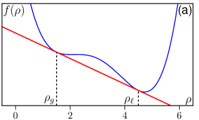
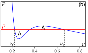
Figure 1: Illustration of the thermodynamic constructions of coexisting densities. (a): Common tangent construction on the free energy density $f(\rho)$. (b): Maxwell equal-area construction on the pressure. In both panels, we used a double-well potential for illustrative purpose.

1.2 Warm-up exercise: the equilibrium limit

Before deriving the binodal curve predicted by Eq. (1) in its most general form, it is illuminating to first review the corresponding equilibrium limit, i.e., the standard Cahn-Hilliard equation [27, 28] which corresponds to $2\lambda+\kappa^{\prime}=0$ [26]. In this case, the dynamics (1) corresponds to a steepest descent in a free energy landscape ${\cal F}[\rho]$:

$$\dot{\rho}=\nabla\cdot\left[M\nabla\frac{\delta{\cal F}}{\delta\rho}\right]\qquad\mbox{where}\qquad{\cal F}[\rho]=\int F[\rho]d{\bf r}=\int\Big{[}f(\rho)+\frac{\kappa(\rho)}{2}(\nabla\rho)^{2}\Big{]}d{\bf r}\;.$$ (3)

$g$ of Eq. (1) is then the chemical potential, defined as the functional derivative of ${\cal F}$ with respect to $\rho$:

$$g=\frac{\delta{\cal F}}{\delta\rho({\bf r})}=g_{0}(\rho)+g_{1}[\rho]\;,$$ (4)

where

$$g_{0}(\rho)=f^{\prime}(\rho)\qquad\mbox{and}\qquad g_{1}[\rho]=-\frac{\kappa^{\prime}(\rho)}{2}(\nabla\rho)^{2}-\kappa(\rho)\Delta\rho\;.$$ (5)

The free energy functional ${\cal F}$ is extensive so that, in a macroscopic phase-separated system, the contribution of the interfaces is sub-dominant. The term $\frac{1}{2}\kappa(\rho)(\nabla\rho)^{2}$ in ${\cal F}$ can then be neglected and the phase equilibria can be determined from the bulk free energy density $f(\rho)$: The coexisting densities $\rho_{g}$ and $\rho_{\ell}$ in the gas and liquid phases are the one minimizing the free energy under the constraint that the average density $\rho_{0}$ is fixed. They are obtained through a common tangent construction on $f(\rho)$ or, equivalently, as the densities satisfying the equalities of chemical potential $f^{\prime}(\rho_{g})=f^{\prime}(\rho_{\ell})=\bar{\mu}$ and pressure $P(\rho_{g})=P(\rho_{\ell})=\bar{P}$, with the pressure $P$ defined as $P(\rho)=\rho f^{\prime}(\rho)-f(\rho)$. Alternatively, the coexisting densities can be constructed using a Maxwell equal area construction

$$\int_{\nu_{\ell}}^{\nu_{g}}\left[{P(\nu)-\bar{P}}\right]d\nu=0$$ (6)

where $\nu\equiv 1/\rho$ is the volume per particle, $\nu_{g/\ell}\equiv 1/\rho_{g/\ell}$. The two thermodynamic constructions are illustrated in Fig. 1.

Note that, instead of relying on a free energy, the equality of pressures and chemical potentials between coexisting phases can also be derived directly from the dynamics (1). First the vanishing of the flux $\mathbf{J}$ in Eq. (1) immediately imposes a uniform chemical potential $g$, which is thus equal between coexisting phases: $g_{0}(\rho_{\ell})=g_{0}(\rho_{g})$. To derive the equality of pressures, we rewrite Eq. (1) as

$$\dot{\rho}=-\nabla\cdot\left[\frac{M}{\rho}\nabla\cdot{\boldsymbol{\sigma}}\right],$$ (7)

where ${\boldsymbol{\sigma}}$ is the stress tensor, whose expression in Cartesian coordinates is

$$\sigma_{\alpha\beta}=-\delta_{\alpha\beta}\left[P(\rho)-\frac{\rho\kappa^{\prime}+\kappa}{2}(\nabla\rho)^{2}-\rho\kappa\Delta\rho\right]-\kappa(\partial_{\alpha}\rho)(\partial_{\beta}\rho)\;.$$ (8)

Note that, similar to $g$, ${\boldsymbol{\sigma}}$ is related to the free-energy functional through [31]:

$${\sigma}_{\alpha\beta}=\delta_{\alpha\beta}\left[F-\rho\frac{\delta{\cal F}}{\delta\rho}\right]-\frac{\partial F}{\partial(\partial_{\beta}\rho)}\partial_{\alpha}\rho.$$ (9)

In fully phase-separated, flux-free steady states, one can get the equality of pressure between coexisting homogeneous phases from Eqs. (7)-(8). For finite systems, Eq. (7) can also be used to derive the finite-size corrections to the binodals due to Laplace pressure [28].

1.3 Generalized thermodynamic variables

For generic functions $\lambda(\rho)$ and $\kappa(\rho)$, which do not satisfy $2\lambda(\rho)+\kappa^{\prime}(\rho)=0$, the free energy structure breaks down because the gradient terms in $g$ cannot be written as a functional derivative:

$$g_{1}[\rho]=\lambda(\rho)(\nabla\rho)^{2}-\kappa(\rho)\Delta\rho\neq\frac{\delta{\cal F}}{\delta\rho}.$$ (10)

A common tangent construction on a free energy density defined through $f^{\prime}(\rho)=g_{0}(\rho)$ then does not lead to the correct coexisting densities [11, 26]. However, as we show below, $g$ can be written as the functional derivative of a generalized free energy ${\cal G}$ with respect to a non-trivial new variable $R$, which depends on the functional forms of $\kappa$ and $\lambda$. Although the dynamics (1) are a priori out of equilibrium, its steady states correspond to extrema of this generalized free energy and, as we show below, we recover the full structure of the equilibrium case described above. We now derive this mapping and show in Section 1.4 how it can be used to compute the binodals of Eq. (1) exactly. Finally, we turn to their finite-size corrections in Section 1.5.

To proceed, we consider the one-to-one mapping $R(\rho)$ defined by

$$\kappa R^{\prime\prime}=-(2\lambda+\kappa^{\prime})R^{\prime}\;,$$ (11)

where the derivatives are taken with respect to $\rho$. Direct inspection shows that $g$ can now be written as a functional derivative with respect to $R$ [26]:

$$g=\frac{\delta{\cal G}}{\delta R}$$ (12)

with

$${\cal G}=\int d{\mathbf{r}}\,G[R]\equiv\int d{\mathbf{r}}\left[\phi(R)+\frac{\kappa}{2R^{\prime}}(\nabla R)^{2}\right]$$ (13)

where we have defined a generalized free energy density $\phi(R)$ such that

$$\frac{d\phi}{dR}=g_{0}\;\qquad\mbox{or alternatively}\qquad\phi=\int^{\rho}g_{0}(\hat{\rho})R^{\prime}(\hat{\rho})d\hat{\rho}\;.$$ (14)

The dynamics of $\rho$ is now written as the derivative of a generalized free energy functional:

$$\dot{\rho}=\nabla\cdot\left[M[\rho]\nabla\frac{\delta{\cal G}}{\delta R}\right]\;.$$ (15)

Note, however, that the structure of (15) differs from the equilibrium case (4) since the functional derivative is taken with respect to $R$ instead of $\rho$. Nevertheless, the steady-state solutions of (15) correspond to extrema of ${\cal G}$ with respect to $R$ .

Comparing Eq. (15) to the equilibrium case (3), we note that the former can be seen as driven by gradients of a generalized chemical potential $g=\frac{\delta{\cal G}}{\delta R}$. Similarly to the equilibrium case, we now show that the dynamics (15) can also be written so as to appear driven by the divergence of a generalized stress tensor. Specifically, the current $\mathbf{J}$ can be rewritten as

$$\mathbf{J}=-M\nabla g=\frac{M}{R}\nabla\cdot\boldsymbol{\sigma}$$ (16)

with a tensor $\boldsymbol{\sigma}$ reading in Cartesian coordinates

$$\sigma_{\alpha\beta} = -\left[h_{0}+Rg_{1}-\frac{\kappa R^{\prime}}{2}(\nabla\rho)^{2}\right]\delta_{\alpha\beta}-\kappa R^{\prime}(\partial_{\alpha}\rho)(\partial_{\beta}\rho)\;,$$ (17)

where we have defined 

$$h_{0}=R\frac{d\phi}{dR}-\phi\;.$$ (18)

Once again, the generalized stress tensor can be deduced from the generalized free energy through

$$\sigma_{\alpha\beta}=\delta_{\alpha\beta}\left[G-R\frac{\delta{\cal G}}{\delta R}\right]-\frac{\partial G}{\partial(\partial_{\beta}R)}\partial_{\alpha}R\;.$$ (19)

In the following, we identify the diagonal coefficients of ${\boldsymbol{\sigma}}$, the normal stresses, with generalized (potentially anisotropic) pressures. Again, we split $h=-\sigma_{xx}$ into a local function and an interfacial contribution:

$$h=h_{0}(\rho)+h_{1}[\rho]\qquad\mbox{where}\qquad h_{1}=Rg_{1}-\frac{\kappa R^{\prime}}{2}(\nabla\rho)^{2}+\kappa R^{\prime}(\partial_{x}\rho)^{2}\;.$$ (20)

We emphasize here that $\boldsymbol{\sigma}$ and $h$ need not have any connection to mechanics and momentum transfer.

Finally, we stress that the equilibrium case is easily recovered using $2\lambda+\kappa^{\prime}=0$: Eq. (11) then implies that $R=\rho$ (up to multiplicative and additive constants that play no role in phase equilibria and can thus be discarded). All our generalized quantities then reduce to their equilibrium counterparts.

Before we turn to the derivation of the binodal curve, we first note that

$$\frac{d^{2}\phi}{dR^{2}}=\frac{g_{0}^{\prime}(\rho)}{R^{\prime}(\rho)}\;.$$ (21)

The spinodal region, defined as $g_{0}^{\prime}(\rho)<0$, thus corresponds to the region in which the generalized free energy density is concave, $\frac{d^{2}\phi}{dR^{2}}<0$, provided $R^{\prime}$ is chosen positive. Furthermore, from Eq. (18) one finds that

$$h_{0}^{\prime}(\rho)=Rg_{0}^{\prime}(\rho)$$ (22)

so that the spinodal region can equivalently be defined from $h_{0}^{\prime}(\rho)<0$. Finally, we note that, contrary to the generalized free energy density $\phi$ which depends on $\lambda$ and $\kappa$ through $R$, the spinodal region is unaffected by the gradient terms in $g$.

We now show how the above results directly yield the binodal curve of our generalized Cahn-Hilliard equation by considering fully phase-separated systems. We then discuss in Section 1.5 the corrections to the binodal curve for finite-size systems.

Figure 2: Schematic representation of the mean density field of a fully phase-separated system in 2d. We consider the density profile connecting gas and liquid phases along a horizontal cut so that the interface is oriented along ${\bf\hat{y}}$ (center). In the macroscopic limit, the interface is locally flat in the transverse direction $\bf\hat{y}$ (left) and the problem simplifies into an effectively 1d domain wall computation for the density profile (right).

1.4 Phase coexistence in the large system size limit

A macroscopic droplet of, say, the dense phase has an infinite radius of curvature in the large system size limit, so that curvature effects are negligible. As in equilibrium, computing the coexisting densities reduces to studying a one-dimensional domain-wall profile perpendicular to the interface [28], whatever the original number of spatial dimensions. To do so, we consider a flat interface, orthogonal to $\mathbf{\hat{x}}$, between coexisting gas and liquid phases at densities $\rho_{g}$ and $\rho_{\ell}$ (see Fig. 2).

For such a profile, any derivative with respect to a direction normal to $\hat{\mathbf{x}}$ vanishes so that Eq. (16) directly implies that $g$ and $\sigma_{xx}$ are constant. For coexisting homogeneous phases, this leads directly to

$$g_{0}(R_{\ell})=g_{0}(R_{g})\qquad\mbox{and}\qquad h_{0}(R_{\ell})=h_{0}(R_{g})$$ (23)

where $R_{\ell,g}\equiv R(\rho_{\ell,g})$. These two constraints thus fully determine the coexisting densities and are equivalent to a common tangent construction on $\phi(R)$ since $g_{0}=\frac{d\phi}{dR}$ and $h_{0}=R\frac{d\phi}{dR}-\phi$.

In stark contrast to equilibrium liquid-gas phase separation, the interfacial terms $g_{1}$ or $h_{1}$ affect the coexisting densities through the definition of $R$, Eq. (11), which depends on $\lambda(\rho)$ and $\kappa(\rho)$. Note that the sole knowledge of the dynamics in Eq. (1) allows us to determine the coexisting densities using the constructions above, without the need to solve for the full density profile at the interface. The common-tangent construction on $\phi$ leads to coexisting densities which are independent of the mean density $\rho_{0}$. The lever rule for determining the phase volumes $V_{\ell}$ and $V_{g}$ therefore still applies: $\rho_{\ell}V_{\ell}+\rho_{g}V_{g}=\rho_{0}V$. Note that this lever rule applies to $\rho$ and not to $R$ since the latter is not a conserved quantity.

The Maxwell construction. As in equilibrium, the common tangent construction on $\phi$ is equivalent to a Maxwell construction on $h_{0}$. We now derive the latter because it will be useful when considering PFAPs, and also since it provides a simpler numerical route to computing the binodal curve from the expression of $h$.

As we shall do for PFAPs, we start from a current given by Eq. (16) so that the flux free condition in a situation as depicted in Fig. 2 implies that the generalized pressure is constant, recalling that the curvature of the interface is negligible:

$$h=h_{0}+h_{1}=\bar{h}$$ (24)

Then, we introduce the generalized volume per particle

$$\upupsilon=\frac{1}{R}$$ (25)

and compute the integral

$$\int_{\upupsilon_{\ell}}^{\upupsilon_{g}}(h_{0}-\bar{h})d\upupsilon=-\int_{x_{g}}^{x_{\ell}}(h_{0}-\bar{h})\partial_{x}\upupsilon dx=\int_{x_{g}}^{x_{\ell}}h_{1}\partial_{x}\upupsilon dx$$ (26)

where the spatial integral is computed along the direction normal to the interface. After some algebra, $h_{1}$ can be rewritten as

$$h_{1}=\frac{1}{R^{\prime}}\left[\left(\kappa-\frac{R\kappa^{\prime}}{R^{\prime}}\right)\frac{(\partial_{x}R)^{2}}{2}-R\kappa\partial_{xx}R\right]+\frac{R\kappa R^{\prime\prime}}{2(R^{\prime})^{3}}(\partial_{x}R)^{2}.$$ (27)

This allows us, after some algebra, to show that $h_{1}\partial_{x}\upupsilon$ is a total derivative

$$h_{1}\partial_{x}\upupsilon=\partial_{x}\left[\frac{\kappa(\partial_{x}R)^{2}}{2RR^{\prime}}\right]\;.$$ (28)

In turn, this leads to a generalized Maxwell construction on $h_{0}$:

$$\int_{\upupsilon_{\ell}}^{\upupsilon_{g}}(h_{0}-\bar{h})d\upupsilon=0\;.$$ (29)

1.5 Finite size effects

Let us now consider what happens if one takes into account the finite curvature of the phase-separated domains. Again, thanks to our mapping, the derivation below resembles closely the one done in equilibrium for the Cahn-Hilliard equation [28]. We consider a radial cut along the interface of a circular domain in 2D, as in Fig 2. By symmetry, the current $\mathbf{J}$ vanishes in steady state. Eq. (16) then immediately gives $\nabla g=0$ so that one still has an equality of generalized chemical potentials between the two phases: $g_{0}(\rho_{g})=g_{0}(\rho_{\ell})$. On the other hand, $\nabla\cdot\boldsymbol{\sigma}=\mathbf{0}$ does not lead to a uniform $\sigma_{xx}$ in this circular geometry, which highlights the different behaviors of the generalized chemical potential and the generalized stress tensor for finite systems.

To proceed, we integrate the radial component of $\nabla\cdot\boldsymbol{\sigma}$ along the path depicted in Fig. 2. To highlight the spherical geometry, we parametrize this path as $r\mathbf{\hat{r}}$. Using the expression for the divergence of a tensor in spherical coordinates (polar in 2D) leads to

$$\int_{r_{\ell}}^{r_{g}}(\nabla\cdot\boldsymbol{\sigma})\cdot\mathbf{\hat{r}}dr=0=\int_{r_{\ell}}^{r_{g}}\left[\partial_{r}\sigma_{rr}+\frac{1}{r}(\sigma_{rr}-\sigma_{\theta\theta})\right]dr$$ (30)

Using the expression (17) of $\boldsymbol{\sigma}$ in this geometry then leads to

$$\sigma_{rr}(r_{\ell})-\sigma_{rr}(r_{g})=h_{0}(\rho_{g})-h_{0}(\rho_{\ell})=-\int_{r_{\ell}}^{r_{g}}\left[\frac{R^{\prime}}{r}\kappa(\partial_{r}\rho)^{2}dr\right]\;,$$ (31)

where we have used that the isotropic terms in $\boldsymbol{\sigma}$ cancel and derivatives with respect to $\theta$ vanish by symmetry.

When the width of the interface is small compared to the droplet radius $r_{d}$, expanding $r$ around $r_{d}$ and using that $(\partial_{r}\rho)^{2}$ vanishes outside the interface leads to

$$\Delta h_{0}\equiv h_{0}(\rho_{\ell})-h_{0}(\rho_{g})\simeq\frac{\gamma}{r_{d}}\;,$$ (32)

where we have introduced a generalized surface tension $\gamma$:

$$\gamma=\int^{r_{g}}_{r_{\ell}}R^{\prime}\kappa(\partial_{r}\rho)^{2}dr\;.$$ (33)

Note that, as for $h_{0}$ and $\sigma$, $\gamma$ need not have any mechanical interpretation for generic phase-separating active matter systems. To leading order in $1/r_{d}$, $\gamma$ can be computed across a flat interface (using a slab geometry as in Fig. 2). For an interface perpendicular to the $x$-axis, it then reads

$$\gamma=\int_{x_{g}}^{x_{\ell}}(\sigma_{yy}-\sigma_{xx})dx=\int_{x_{g}}^{x_{\ell}}R^{\prime}\kappa(\partial_{x}\rho)^{2}dx.$$ (34)

Finally, let us comment on the sign of $\gamma$ which has recently attracted interest since it has been measured negative for PFAPs [32] (see Section 3.4 for a discussion of that case). Here, since $\kappa$ need to be positive for stability reasons, we see from Eq. (34) that $\gamma$ has the sign of $R^{\prime}$. Starting from the dynamics in Eq. (1), the sign of $R^{\prime}$ is arbitrary, corresponding to an integration constant when solving Eq. (11). The generalized surface tension $\gamma$ can then be either positive or negative, although with different expressions for the generalized pressure $h_{0}(\rho)$. On the other hand, starting from an expression for the stress tensor in Eq. (17), as will be the case for PFAPs in Section 3, $R^{\prime}$ is fixed by the expression for $\boldsymbol{\sigma}$ and can take either sign. Our framework thus supports both positive and negative $\gamma$.

1.6 Illustration of our general framework for a scalar active matter model

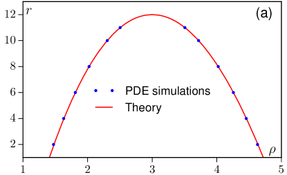
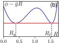
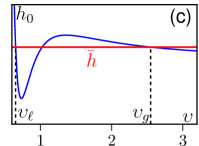
Figure 3: (a): Binodals measured in 2d simulations of Eq. (1) with the coefficients of Eq. (35) compared to the theoretical predictions of Eq. (23). (b): Common tangent construction on $\phi(R)$ for $r=2$. (c): Maxwell construction on $h_{0}(\upupsilon)$, Eq. (29) for $r=2$. Eq. (1) was integrated with a precision of $dx=1$ in space and a time step $dt=2.5\times 10^{-4}$ for a system size of $100\times 20$.

In this section we show on a particular example that our generalized thermodynamic construction predicts exactly the phase equilibria of our nonequilibrium Cahn-Hilliard equation (1) through Eq. (23). To this end, we numerically integrate this equation in 2d for the particular (and rather arbitrary) choice:

$$g_{0}(\rho)=r(\rho-\rho_{0})-12(\rho-\rho_{0})^{2}+4(\rho-\rho_{0})^{3}\,;\quad M=1\,;\quad\kappa(\rho)=\rho\,;\quad\lambda=0.$$ (35)

To check the theory, we first numerically solve Eqs. (1) and (35) using a semi-spectral integration scheme (linear terms are computed in Fourier space, non-linear terms in real space) with Euler time stepping. For each value of $r$, we start from a phase-separated state with two arbitrarily chosen densities ($\rho_{g}=1$ and $\rho_{\ell}=5$) and measure the coexisting densities once the system has relaxed to its steady state.

To compare with the theoretical predictions for the binodals, we first determine the function $R(\rho)$ using Eq. (11), which (up to two unimportant integration constants) gives $R(\rho)=\log\rho$. We then use either the common tangent construction on $\phi(R)$ or the Maxwell construction on $h_{0}(\upupsilon)$, shown in Fig. 3(b,c), as described in the previous section. The comparison with the coexistence densities measured in the simulations of Eq. (1) is shown in Fig. 3(a): the difference between theory and simulations is found to be smaller than $0.5$% for every point, thus confirming that the dynamics does indeed yield the stationary state analyzed in Section 1.

These numerical results are obtained in systems where a straight band of liquid coexists with a dilute gas phase so that finite-size curvature effects are negligible. On the contrary, when finite-size liquid droplets coexist with a gaseous background, the coexisting densities differ from those predicted by Eq. (23) due to the finite-size corrections discussed in Section 1.5. In this case, a jump of the generalized pressure through the interface is indeed measured numerically, and found to be given quantitatively by the generalized surface tension (33) (See Fig. 4a). Similarly, there are density shifts in each of the phases which scale as $1/r_{d}$ as shown in Fig. 4b.

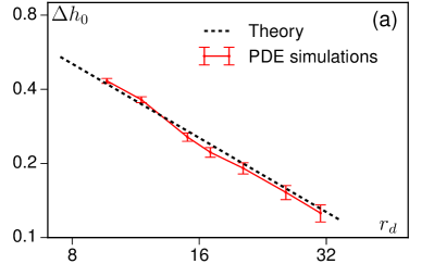
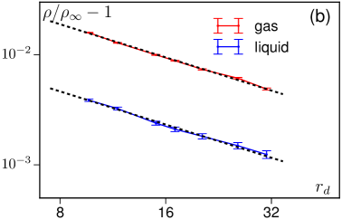
Figure 4: Finite size effects measured in 2d simulations of Eqs. (1) and (35) with $r=2$. (a): Difference in the generalized pressure $h_{0}$ between the two phases. The dashed line is the predicted leading order behavior $\gamma/r_{d}$ with the effective surface tension $\gamma=4.06$ measured independently from a straight interface using Eq. (33). (b): Corrections to the coexisting densities. The dashed lines are fits to $c_{g,\ell}/r_{d}$ with $c_{g,\ell}$ a phase dependent constant. The system size is $80\times 80$, and the other parameters as in Fig. 3.

2 QSAPs.

We now turn to a microscopic model for QSAPs, for which we derive a hydrodynamic description and compare the predictions of our formalism with direct numerical simulations of the microscopic model. We consider particles labeled by $i=1\dots N$, moving at speed $v$ along body-fixed directions $\mathbf{u}_{i}$ which undergo both continuous rotational diffusion with diffusivity $D_{r}$ and complete randomization with tumbling rate $\alpha$. The equations of motion are given by the Langevin dynamics

$$\dot{{\bf r}}_{i} =v\left[\tilde{\rho}({\bf r}_{i}+\varepsilon{\bf u}_{i})\right]{\bf u}_{i}+\sqrt{2D_{t}}\boldsymbol{\eta}_{i}$$ (36)

$$\dot{\theta}_{i} =\sqrt{2D_{r}}\xi_{i}+\sum_{j}\delta(t-t_{j})\delta\theta_{j}$$

where $\boldsymbol{\eta}$ and $\xi$ are delta-correlated Gaussian white noises of appropriate dimensionality. In addition to continuous angular diffusion, we have included in (36) a non-Gaussian noise accounting for tumbling events: the $t_{i}$ are Poisson distributed with a rate $\alpha$ and the $\delta\theta_{j}$’s are drawn from a uniform distribution between $0$ and $2\pi$. Each particle adapts its speed, $v[\tilde{\rho}(\mathbf{r}_{i}+\varepsilon\mathbf{u}_{i})]$, to a local measurement of the density:

$$\tilde{\rho}(\mathbf{r}+\varepsilon\mathbf{u}_{i})=\int d\mathbf{r}^{\prime}K(\mathbf{r}+\varepsilon\mathbf{u}_{i}-\mathbf{r}^{\prime})\hat{\rho}(\mathbf{r}^{\prime})d\mathbf{r}^{\prime}$$ (37)

with $K(\mathbf{r})$ an isotropic coarse-graining kernel, and $\hat{\rho}(\mathbf{r})=\sum_{i}\delta(\mathbf{r}-\mathbf{r}_{i})$ the microscopic particle density. Note that the local density is measured with an offset $\varepsilon\mathbf{u}_{i}$ which allows for anisotropic quorum sensing. This effect, which does not create alignment interactions, captures a slowdown of particles that would arise, for instance, due to a large density of particles in front of them. This can thus model, say, a visual quorum-sensing or steric hindrance. In a different context, anisotropic sensing has been shown to lead to a rich phenomenology for aligning active particles [33].

2.1 Hydrodynamic description of QSAPs.

Deriving hydrodynamic equations from microscopics is generally difficult, even in equilibrium [34]. For QSAPs we can follow the path of [1, 24, 35], taking a mean-field approximation of their fluctuating hydrodynamics. We first assume a smooth density field and a short-range anisotropy so that the velocity can be expanded as

$$v(\tilde{\rho})\simeq v(\rho)+\varepsilon v^{\prime}(\rho)\nabla\rho\cdot\mathbf{u}_{i}+\ell^{2}v^{\prime}(\rho)\Delta\rho+{\cal O}(\varepsilon^{2},\nabla^{3})$$ (38)

where $\rho$ is evaluated at ${\bf r}_{i}$ and $\ell^{2}=\int r^{2}K(\mathbf{r})d\mathbf{r}$. Following [24, 35], the fluctuating hydrodynamics of QSAPs, derived in A, is then given by:

$$\dot{\rho}=\nabla\cdot(M\nabla g+\sqrt{2M\rho}{\bf\Lambda})$$ (39)

with ${\bf\Lambda}$ a unit Gaussian white noise vector and

$$g_{0}(\rho)=\log(\rho v)+\frac{\varepsilon}{\tau v};\quad M=\rho\frac{\tau v(\tilde{\rho})^{2}}{d};\quad\kappa(\rho)=-\ell^{2}\frac{v^{\prime}}{v}\left(1-\frac{\varepsilon}{\tau v}\right);\quad\lambda(\rho)=0\;,$$ (40)

where $d$ is the number of spatial dimensions. Here, $\tau\equiv[(d-1)D_{r}+\alpha]^{-1}$ is the orientational persistence time. The mean-field hydrodynamic equation of QSAPs is then Eq. (1) with the coefficients in Eq. (40). As mentioned earlier, the spinodal region is defined from the criterion $g_{0}^{\prime}(\rho)<0$, which leads here to a modification of the standard linear instability criterion for QSAPs [1]:

$$\frac{v^{\prime}(\rho)}{v(\rho)}\left(1-\frac{\varepsilon}{\tau v}\right)<-\frac{1}{\rho}\;.$$ (41)

To construct the phase diagram for a given choice of $v(\rho)$, using the generalized thermodynamic procedure, we first solve for $R(\rho)$ using Eq. (11) and from it obtain both $\phi(R)$ and $h_{0}(R)$. The binodals then follow via a common-tangent construction on $\phi(R)$ or, equivalently, by setting equal values of $h_{0}$ and $g_{0}$ in coexisting phases. Note that since $2\lambda+\kappa^{\prime}\neq 0$ one has $R\neq\rho$. The phase diagram thus cannot be found by globally minimizing a free energy density $f(\rho)$ defined from $f^{\prime}(\rho)=g_{0}(\rho)$ as discussed before [1, 24]. Indeed, such a procedure correctly captures the equality of $g_{0}$ in both phases but predicts a common tangent construction on $f$ which is violated. We now turn to describe the numerical simulations of microscopic models of QSAPs.

2.2 Comparison between theory and numerics.

In what follows we study models where the density $\tilde{\rho}$ is computed according to Eq. (37) with the bell-shaped kernel

$$K(r)=\frac{\Theta(r_{0}-r)}{Z}\exp\left(-\frac{r_{0}^{2}}{r_{0}^{2}-r^{2}}\right)\;.$$ (42)

Here $\Theta$ is the Heaviside function, $Z$ a normalization constant and we used an interaction radius of $r_{0}=1$. In addition we take the velocity to be

$$v(\rho)=v_{0}+\frac{v_{1}-v_{0}}{2}\left[1+\tanh\left(2\frac{\rho}{\rho_{m}}-2\right)\right]\;.$$ (43)

This interpolates smoothly between a high velocity $v_{0}$ at low density ($\rho\ll\rho_{m}$) and a low velocity $v_{1}$ at high density ($\rho\gg\rho_{m}$). In addition to the 2d continuous space model described above, we also conducted simulations of QSAPs in 1d on lattice [2]. In this case, we consider run-and-tumble particles (RTPs): particle $i$ has a direction of motion $u_{i}=\pm 1$ which is flipped at rate $\alpha/2$. It then jumps on the lattice site in direction $u_{i}$ with rate $v[\tilde{\rho}(x_{i}+\varepsilon u_{i})]$.

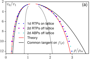
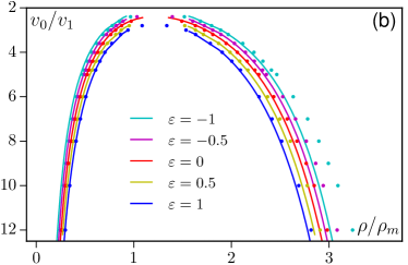
Figure 5: Phase diagrams of QSAPs. (a) Symmetric sensing ($\varepsilon=0$). The solid lines correspond to common tangent constructions on $\phi(R)$ (red) or $f(\rho)$ (black). Dashed lines correspond to the spinodals $d^{2}\phi/dR^{2}=d^{2}f/d\rho^{2}=0$. Data points are from simulations of RTPs ($\alpha=1,\,D_{r}=0$) and ABPs ($\alpha=0,\,D_{r}=1$), either in 1d on lattice (system size $L=2000$ lattice sites) or in a 2d continuous space (system size $50\times 50$). (b) Asymmetric sensing ($\varepsilon\neq 0$) for 1d RTPs on lattice: Solid lines show the predicted binodals computed by common tangent constructions on $\phi(R)$, and symbols denote simulation results obtained with systems of size $L=2000$ lattice sites. For all plots, we used $\rho_{m}=200$, $v_{1}=5$, $\tau=1$.

Fig. 5a shows the phase diagrams predicted by our generalized thermodynamics and those measured in QSAP simulations for a symmetric sensing of the density ($\varepsilon=0$). Overall, the agreement between predicted and measured binodals is excellent, in contrast to the common tangent construction on $f(\rho)$. It is remarkable that, for QSAPs, we can quantitatively predict the phase diagram of a microscopic model without any fitting parameters, something rare even for equilibrium models.

Fig. 5b shows the binodals measured in 1d simulations on lattice with $\varepsilon\neq 0$ together with the corresponding theoretical predictions. The dependence of the binodals on the asymmetry $\varepsilon$ is apparent in both cases. It results from the explicit dependence of $g_{0}(\rho)$ on $\varepsilon$ established in Eq. (40). This dependence probably explains why run-and-tumble particles hopping on lattices with excluded-volume interactions [2] are not well described by the coarse-grained theory proposed so far for QSAPs which did not account for any asymmetric sensing [1]. We can see that our theoretical predictions are more accurate for small $\varepsilon$, as expected from the derivation of the hydrodynamic equation given in A.

Our theoretical predictions for the phase diagram of QSAPs rely on two different approximations. First, we use a mean-field approximation to derive the specific expression (40) for $g[\rho]$. For our choice of $v(\rho)$, MIPS occurs only at large densities so that this approximation works very well except in the small and numerically unresolved Ginzburg interval close to the critical point. Second, our general theory disregards higher order gradient terms in Eq. (1). This probably explains why the hydrodynamic description works best fairly close to the critical point, where interfaces are smoothest and the gradient expansion, Eq. (38), most accurate. The quantitative limitations of our gradient expansion highlights that gradient terms directly influence the coexisting densities through Eq. (11), unlike the equilibrium case.

In addition to giving quantitative predictions for the phase diagrams, our approach sheds light on the observed universality of the MIPS in QSAPs. For example, the phase diagram does not depend on the exact shape of the kernel $K$, which enters Eq. (40) through $\ell^{2}$ which then cancels in the nonlinear transform $R(\rho)$. Similarly, Fig. 5 also shows lattice simulations of QSAPs in $1d$ where complete phase separation is replaced by alternating domains (with densities given by the predicted binodal values). This confirms the equivalence of continuous (ABP) and discrete (RTP) angular relaxation dynamics for QSAPs [24, 35]. Our results, however, also expose sensitivity to other microscopic parameters such as the fore-aft asymmetry $\varepsilon$ which enters $g_{0}$ and therefore affects the binodals. This might explain the different collective behaviors seen in swarms of robots that adapt their speeds to the density sampled in either the forward or the backward direction [36].

2.3 Finite-size corrections.

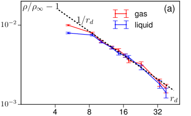
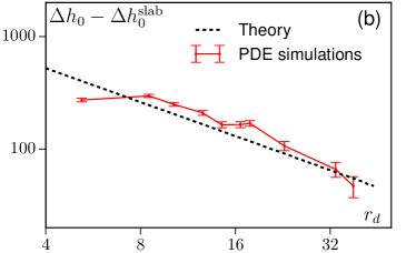
Figure 6: Finite size effects in phase-separated QSAPs, measured in 2d off-lattice simulations of QSAPs with symmetric sensing ($\varepsilon=0$). (a): Correction to the coexisting densities. The dashed line shows a scaling proportional to $1/r_{d}$. (b): Correction to the generalized pressure $h_{0}$. The dashed line is the predicted leading order behavior $\gamma/r_{d}$ with the effective surface tension $\gamma$ measured independently across a straight interface using Eq. (33). $\Delta h_{0}^{\rm slab}$ accounts for the small pressure jump due to Eq. (40) not being exact, as described in the text. The simulation parameters are $\rho_{m}=50$, $v_{0}=30$, $v_{1}=5$, $\tau=1$ and a system size $100\times 100$.

Similar to the scalar active model of Section 1.6, we expect finite size corrections when a liquid droplet is formed in a finite system: for a droplet of radius $r_{d}$, we expect to leading order in the droplet radius an effective pressure jump across the interface (32):

$$\Delta h_{0}(r_{d})\simeq\frac{1}{r_{d}}\int^{r_{g}}_{r_{\ell}}\frac{\kappa}{R^{\prime}}(\partial_{r}R)^{2}dr\;.$$ (44)

Accordingly, one expect the finite-size corrections to the co-existing densities to decay as $\propto 1/r_{d}$. In Fig. 6a, we show that the measured binodals indeed converge towards their asymptotic values in a manner consistent with a $1/r_{d}$ decay.

A quantitative check of (44) is difficult since, first, our derivation of $h_{0}(R(\rho))$ is based on a number of approximations, and, second, our numerical measurements of the binodals are necessarily noisy. To proceed, we measure $\rho_{g}(r_{d})$ and $\rho_{\ell}(r_{d})$ and construct $\Delta h_{0}(r_{d})=h_{0}(\rho_{\ell}(r_{d}))-h_{0}(\rho_{g}(r_{d}))$. $\Delta h_{0}(r_{d})$ does not vanish exactly in the large system size limit, nor in a slab geometry in which we measure a small correction $\Delta h_{0}^{\rm slab}/h_{0}(\rho_{\ell})\approx 0.1\%$. This systematic error can stem from several origins, from the gradient expansion to the mean-field approximation, through limitations in the numerical accuracy of the density measurement. Though very small, this error becomes comparable to the Laplace pressure jump for radii $r_{d}\apprge 20$, highlighting the numerical challenges in measuring these finite-size effects. Nevertheless we show in Fig. 6b that $\Delta h_{0}(r_{d})-\Delta h_{0}^{\rm slab}$ converges to its asymptotic value consistently with a $1/r_{d}$ decay. Furthermore, the prediction of Eq. (44) can be checked by measuring the prefactor $\gamma\equiv\int_{r_{g}}^{r_{\ell}}\frac{\kappa}{R^{\prime}}(\partial_{r}R)^{2}dr$ of this decay in a slab geometry. The corresponding prediction is shown as a dashed line in Fig. 6b and agrees semi-quantitatively with our numerical results, without any fitting parameters.

To understand why we observe a quasi-quantitative agreement despite relatively small values of $r_{d}$, it is useful to explicitly expand Eq. (31) as

$$\Delta h_{0}\simeq\frac{1}{r_{d}}\int_{r_{\ell}}^{r_{g}}drR^{\prime}\kappa(\partial_{r}\rho)^{2}\left(1-\frac{r-r_{d}}{r_{d}}+\frac{(r-r_{d})^{2}}{r_{d}^{2}}\right)\;.$$ (45)

The first order correction to $\Delta h_{0}=\frac{\gamma}{r_{d}}$ is thus given by

$$\Delta h_{0}-\frac{\gamma}{r_{d}}=-\frac{1}{r_{d}^{2}}\int_{r_{\ell}}^{r_{g}}drR^{\prime}\kappa(\partial_{r}\rho)^{2}(r-r_{d}).$$ (46)

Using that, from the definition (11), $(R^{\prime}\kappa)^{\prime}=-2\lambda R^{\prime}$, the prefactor $R^{\prime}\kappa$ can then be expanded around $r=r_{d}$ as

$$R^{\prime}[\rho(r)]\kappa[\rho(r)]\simeq R^{\prime}[\rho(r_{d})]\kappa[\rho(r_{d})]-2\partial_{r}\rho(r_{d})(r-r_{d})\lambda[\rho(r_{d})]\kappa^{\prime}[\rho(r_{d})].$$ (47)

Since $\lambda=0$ for QSAPs, we are left with

$$\Delta h_{0}-\frac{\gamma}{r_{d}}=-\frac{R^{\prime}[\rho(r_{d})]\kappa[\rho(r_{d})]}{r_{d}^{2}}\int_{r_{\ell}}^{r_{g}}dr(\partial_{r}\rho)^{2}(r-r_{d}),$$ (48)

which is zero for a symmetric interface so that in that case

$$\Delta h_{0}=\frac{\gamma}{r_{d}}\left[1+{\cal O}\left(\frac{1}{r_{d}^{2}}\right)\right].$$ (49)

For our choice of $v(\rho)$, the density profile is indeed very close to a hyperbolic tangent (data not shown) and the lack of first order corrections for such profiles probably explains the semiquantitative agreement of our numerical results with the $1/r_{d}$ behaviour.

3 PFAPs.

We now consider the case of self-propelled particles interacting via pairwise forces, which has attracted considerable interest over the past few years [3, 4, 29, 8, 37, 25, 17, 38]. We define the model in Section 3.1 and construct its hydrodynamic description in Section 3.2. Contrary to QSAPs, there is no available method to derive accurate estimates of the coefficients $\lambda(\rho)$ and $\kappa(\rho)$ or to rule out the existence of other terms [30]. We discuss in Section 3.3 how we can nevertheless follow the path laid out using our generalized thermodynamic formalism to understand how coexistence densities are selected in PFAPs. Finally, finite-size effects are considered in Section 3.4.

3.1 Model.

We consider $N$ self-propelled particles in two dimensions interacting via the repulsive, pairwise additive, Weeks-Chandler-Andersen potential:

$$V(r)=4\epsilon\!\left[\left(\frac{\sigma}{r}\right)^{12}-\left(\frac{\sigma}{r}\right)^{6}\right]\!+\epsilon$$ (50)

with an upper cut-off at $r=2^{1/6}\sigma$, beyond which $V=0$. Here $\sigma$ defines the particle diameter, $\epsilon$ determines the interaction strength, and $r$ is the center-to-center separation between two particles. Particle $i$ evolves in two dimensions, with periodic boundary conditions, according to the Langevin equations:

$$\dot{{\bf r}}_{i}=-\mu\sum_{j}\nabla_{i}V(|{\bf r}_{i}-{\bf r}_{j}|)+\sqrt{2D_{t}}{\boldsymbol{\xi}}_{i}+v_{0}{\bf u}_{i};\qquad\dot{\theta}_{i}=\sqrt{2D_{r}}\eta_{i}.$$ (51)

Here, ${\bf u}_{i}=(\cos\theta_{i},\sin\theta_{i})$ indicates the direction of self-propulsion and $\eta_{i},{\boldsymbol{\xi}}_{i}$ are unit Gaussian white noises. For simplicity, we only include continuous rotational diffusion but our results are expected to extend to run-and-tumble dynamics since these two types of orientational noise have been shown to lead to the same phase diagram [35].

The full phenomenology of this model requires scanning a three-parameter phase diagram, parametrized for instance by the Péclet number ${\rm Pe}=3v_{0}/(\sigma D_{r})$ , the packing fraction $(\pi/4)\sigma^{2}\rho$ and the potential stiffness $\mu\epsilon/(v_{0}\sigma)$. Here, we focus on the onset of MIPS as the Péclet number and the packing fraction are varied, disregarding the role of the potential stiffness [3, 4, 5, 39]. In practice, we fix $\epsilon=1,\sigma=1,v_{0}=24,\mu=1$ and vary $D_{r}$ and $\rho$. MIPS then occurs at high enough densities when the run-length $v_{0}/D_{r}$ is much larger than the particle size $\sigma$, namely when ${\rm Pe}$ exceeds a threshold value ${\rm Pe}_{c}\approx 50$ [3, 4, 5, 6].

3.2 Hydrodynamic description.

Following [40, 17], we start from the exact Itō-Langevin equation for the microscopic density of particles $\hat{\psi}({\bf r},\theta)=\sum_{i=1}^{N}\delta({\bf r}-{\bf r}_{i})\delta(\theta-\theta_{i})$ at position ${\bf r}$ with orientation $\theta$

$$\partial_{t}\hat{\psi}=-\nabla\cdot\left[v_{0}\mathbf{u}\hat{\psi}+\hat{\mathbf{I}}^{(\theta)}-D_{t}\nabla\hat{\psi}+\sqrt{2D_{t}\hat{\psi}}\boldsymbol{\eta}\right]+\partial_{\theta}\left[D_{r}\partial_{\theta}\hat{\psi}+\sqrt{2D_{r}\hat{\psi}}\xi\right]$$ (52)

where $\hat{\mathbf{I}}^{(\theta)}(\mathbf{r},\theta)=-\int d\mathbf{r}^{\prime}\mu\nabla V(|\mathbf{r}^{\prime}-\mathbf{r}|)\hat{\rho}(\mathbf{r}^{\prime})\hat{\psi}(\mathbf{r},\theta)$, $\hat{\rho}({\bf r})=\int\hat{\psi}(\mathbf{r},\theta)d\theta$ is the fluctuating density, and $\boldsymbol{\eta}$ and $\boldsymbol{\xi}$ are unit-variance Gaussian white noises of appropriate dimensionality. Denoting averages over noise realizations by angular brackets we define $\rho(\mathbf{r})=\langle\hat{\rho}(\mathbf{r})\rangle$, $\mathbf{m}(\mathbf{r})=\langle\hat{\mathbf{m}}(\mathbf{r})\rangle$ and $\mathds{Q}({\bf r})=\langle\hat{\mathds{Q}}({\bf r})\rangle$. Here $\hat{\mathbf{m}}(\mathbf{r})=\int d\theta\mathbf{u}\hat{\psi}(\mathbf{r},\theta)$, is the orientation vector, $\hat{\mathds{Q}}({\bf r})=\int d\theta\left({\bf u}:{\bf u}-\mathds{1}/2\right)\hat{\psi}(\mathbf{r},\theta)$, is the nematic tensor, and $\mathds{1}$ the identity matrix.

Integrating Eq. (52) over $\theta$ and averaging over noise realizations, the dynamics of $\rho(\mathbf{r},t)$ reads

$$\partial_{t}\rho=-\nabla\cdot\mathbf{J};\quad\mathbf{J}=v_{0}\mathbf{m}+\mathbf{I}^{(0)}-D_{t}\nabla\rho$$ (53)

with

$$\mathbf{I}^{(0)}(\mathbf{r})=\left\langle\int d\theta\hat{\mathbf{I}}^{(\theta)}(\mathbf{r},\theta)\right\rangle=-\int d\mathbf{r}^{\prime}\mu\nabla V(|\mathbf{r}-\mathbf{r}^{\prime}|)\langle\hat{\rho}({\bf r})\hat{\rho}({\bf r}^{\prime})\rangle\;.$$ (54)

The dynamics of $\mathbf{m}$ is then obtained similarly by multiplying Eq. (52) by ${\bf u}$ and integrating over $\theta$. This yields, with an implied summation over repeated indices,

$$\partial_{t}m_{\alpha}=-\partial_{\beta}\left[v_{0}\left(\mathds{Q}_{\alpha\beta}+\frac{\rho\delta_{\alpha\beta}}{2}\right)+\mathds{I}^{(1)}_{\alpha\beta}-D_{t}\partial_{\beta}m_{\alpha}\right]-D_{r}m_{\alpha}$$ (55)

where the last term is obtained by integration by parts and we have defined

$$\mathds{I}^{(1)}_{\alpha\beta}=-\int d\mathbf{r}^{\prime}\mu\partial_{\beta}V(|\mathbf{r}-\mathbf{r}^{\prime}|)\langle\hat{\rho}(\mathbf{r}^{\prime})\hat{m}_{\alpha}(\mathbf{r})\rangle\;.$$ (56)

We stress that, so far, Eq. (52) and (55) are exact, although they are not closed since they feature $\mathds{Q}$ and the microscopic correlators in $\mathbf{I}^{(0)}$ and $\mathds{I}^{(1)}$ which depend on higher moments of $\hat{\psi}$.

As a first approximation, we use that, contrary to $\rho(\mathbf{r},t)$, $\mathbf{m}$ is a fast mode decaying at a rate $D_{r}$. On time scales much larger than $D_{r}^{-1}$, one can thus assume that $m_{\alpha}$ relaxes locally to

$$m_{\alpha}=-\frac{1}{D_{r}}\partial_{\beta}\left[v_{0}\left(\mathds{Q}_{\alpha\beta}+\frac{\rho\delta_{\alpha\beta}}{2}\right)+\mathds{I}^{(1)}_{\alpha\beta}-D_{t}\partial_{\beta}m_{\alpha}\right].$$ (57)

The current in Eq. (53) is then given by

$$J_{\alpha}=-\left[D_{t}+\frac{v_{0}^{2}}{2D_{r}}\right]\partial_{\alpha}\rho-\frac{v_{0}}{D_{r}}\partial_{\beta}\mathds{I}^{(1)}_{\alpha\beta}+I^{(0)}_{\alpha}-\frac{v_{0}^{2}}{D_{r}}\partial_{\beta}\mathds{Q}_{\alpha\beta}+\frac{D_{t}v_{0}}{D_{r}}\partial_{\beta\beta}m_{\alpha}\;.$$ (58)

Interestingly, Eq. (58) can be rewritten as the divergence of a stress tensor

$$J_{\alpha}=\mu\partial_{\beta}\sigma_{\alpha\beta}$$ (59)

with

$$\sigma_{\alpha\beta}=-\left[\frac{D_{t}}{\mu}+\frac{v_{0}^{2}}{2\mu D_{r}}\right]\rho\delta_{\alpha\beta}-\frac{v_{0}}{\mu D_{r}}\mathds{I}^{(1)}_{\alpha\beta}+\sigma^{\rm IK}_{\alpha\beta}-\frac{v_{0}^{2}}{\mu D_{r}}\mathds{Q}_{\alpha\beta}+\frac{D_{t}v_{0}}{\mu D_{r}}\partial_{\beta}m_{\alpha}$$ (60)

where we have followed Irving and Kirkwood [41] (and Ref.[31] in a similar context) and write $I^{(0)}_{\alpha}=\mu\partial_{\beta}\sigma^{\rm IK}_{\alpha\beta}$ with

$$\sigma^{\rm IK}_{\alpha\beta}({\bf r})=\frac{1}{2}\int d{\bf r}^{\prime}\frac{({\bf r}-{\bf r}^{\prime})_{\alpha}({\bf r}-{\bf r}^{\prime})_{\beta}}{|{\bf r}-{\bf r}^{\prime}|}\frac{dV(|{\bf r}-{\bf r}^{\prime}|)}{d|{\bf r}-{\bf r}^{\prime}|}\int_{0}^{1}d\lambda\langle\hat{\rho}({\bf r}+(1-\lambda){\bf r}^{\prime})\hat{\rho}({\bf r}-\lambda{\bf r}^{\prime})\rangle\;.$$ (61)

We now turn to relate these results to the formalism derived previously.

Generalized pressure and equation of state.

The resulting dynamics for $\rho$, with the current given by Eq. (59), should be compared to the generalized Cahn-Hilliard equation of Section 1 with the current driven by the generalized stress tensor as in Eq. (16). We see that PFAPs correspond to the special case $M/R=\mu$, the microscopic mobility. This has important consequences for the mechanical interpretation of $\boldsymbol{\sigma}$. Indeed, one can see that imposing an external potential $U$ on the particles leads to

$$\mathbf{J}=\mu\nabla\cdot\boldsymbol{\sigma}-\mu\rho\nabla U\;.$$ (62)

In a flux free steady state, $\mathbf{J}=\mathbf{0}$ and Eq. (62) becomes a force balance. Integrating (62) from a point in the bulk to infinity shows the normal component of $\boldsymbol{\sigma}$ to be equal to the total force per unit area exerted on a boundary. Indeed, the normal component of $\boldsymbol{\sigma}$ exactly coincides in homogeneous phases with the equation of state (EOS) found previously for the mechanical pressure $P$ of PFAPs [17]. Generalized and mechanical pressure thus coincide for PFAPs and we note, following Section 1.1

$$h\equiv-{\sigma}_{xx}=\frac{D_{t}}{\mu}\rho+P^{A}(x)+P^{D}(x)+\frac{v_{0}^{2}}{\mu D_{r}}\mathds{Q}_{xx}-\frac{D_{t}v_{0}}{\mu D_{r}}\partial_{x}m_{x}$$ (63)

where we have defined, following earlier notation [17], the “active” contribution to the pressure $P^{A}$ and a “direct” passive-like part $P^{D}$:

$$P^{A}=\frac{v_{0}^{2}}{2\mu D_{r}}\rho+\frac{v_{0}}{\mu D_{r}}\mathds{I}^{(1)}_{xx};\qquad P^{D}=-\sigma^{\rm IK}_{xx}.$$ (64)

Note that $P^{A}$ is sometimes also called “swim pressure” [12], even though neglecting the pressure of the surrounding fluid to describe the phase separation of actual swimmers is problematic.

The value of the pressure in a homogeneous phase of density $\rho_{0}$ is then given by

$$h\left[\rho(x)=\rho_{0}\right]\equiv h_{0}(\rho_{0})=\rho_{0}\frac{D_{t}}{\mu}+P^{A}_{0}+P^{D}_{0}\;,$$ (65)

where $P^{A}_{0}$ and $P^{D}_{0}$ are the values taken by $P^{A}$ and $P^{D}$ in homogeneous disordered phases of density $\rho_{0}$. This allows us to identify, in analogy with Eq. (20),

$$h=h_{0}(\rho(x))+h_{1}([\rho],x)\;.$$ (66)

Note that while the structure is similar to Eq. (20), there is no gradient expansion taken here – $h_{1}$ is exact, formally containing gradients of all orders. Its expression is given by

$$h_{1}=P^{A}_{1}[\rho]+P^{D}_{1}[\rho]+\frac{v_{0}^{2}}{\mu D_{r}}{\mathds{Q}_{xx}}-\frac{D_{t}v_{0}}{\mu D_{r}}\partial_{x}m_{x}.$$ (67)

where $P^{A/D}_{1}\equiv P^{A/D}-P^{A/D}_{0}$ contains the interfacial contributions to the active and the direct pressures. The terms in $m_{x}$ and $\mathds{Q}_{xx}$ are purely interfacial since they vanish in the (disordered) bulk phases. We now show that the phase equilibria in PFAPs can be understood using these results with the ideas of Section 1.

3.3 Phase equilibria in PFAPs.

One way forward would be to construct an explicit gradient expansion for $h$ in terms of $\rho$ and obtain closed expressions for $h_{0}$ and $h_{1}$. This would then allow us to find $R(\rho)$ and $\phi(R)$ analytically as was done for QSAPs in Section 2. Despite the extensive literature on PFAPs, such a gradient expansion has not yet been presented, but could be accomplished for instance by using a low-density virial approximation. Such a route would possibly lead to qualitative predictions for the phase diagram, but our goal here is to show that our formalism quantitatively accounts for the phase equilibria of PFAPs, and we thus do not want to rely on such approximations. We thus proceed differently, using an approach where we instead measure the gradient terms to quantitatively verify the validity of our formalism for PFAPs.

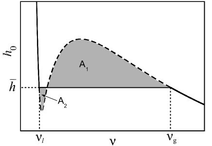
Figure 7: Schematic picture of the violation of the Maxwell equal area construction. The black non-monotonic line shows the equation of state $h_{0}(\nu)$, dashed in the part where homogeneous systems are unstable with respect to phase separation. The violation of the Maxwell equal-area construction is quantified by $\Delta A=A_{1}-A_{2}\neq 0$.

As with the other systems, we first consider the case of a macroscopically phase separated system, for which the liquid-gas interface is locally flat and perpendicular to $\mathbf{\hat{x}}$. As in Section 1.4, in a flux-free steady state, $h=\bar{h}$ is constant across the interface so that the pressure is equal in coexisting phases

$$h_{0}(\rho_{g})=h_{0}(\rho_{\ell})=\bar{h}.$$ (68)

To construct the phase diagram, we need to complement this equality by a second constraint. Since we do not have any closed expression for the interfacial terms $h_{1}$, we cannot use a Maxwell construction in the $(h_{0},\upupsilon=R^{-1})$ plane as was done in Section 1.4. Instead, we measure the violation of the equilibrium Maxwell construction in the $(h_{0},\nu\equiv\rho^{-1})$ plane, schematically depicted in Fig. 7, with $\nu=1/\rho$ the free volume per particle:

$$\int_{\nu_{\ell}}^{\nu_{g}}(h_{0}(\nu)-\bar{h})d\nu=\int_{x_{g}}^{x_{\ell}}h_{1}\,\partial_{x}\nu\,dx\equiv\Delta A\;.$$ (69)

Here $h_{0}(\nu)$ is the pressure-volume EOS, $\bar{h}$ is the pressure of coexisting phases and $\Delta A\neq 0$ directly quantifies the violation of the Maxwell construction for PFAPs [17].

Given the value of $\Delta A$, Eqs (68) and (69) are two independent constraints satisfied by $\rho_{\ell}$ and $\rho_{g}$. A fully predictive theory would thus evaluate $\Delta A$ analytically and then solve (68) and (69) to obtain the values of the binodals and the coexisting pressure $\bar{h}$. Here, instead, we use a numerical measurement of $\Delta A$ to construct the phase diagram. Although less predictive than knowing $h_{0}$ and $h_{1}$ analytically, our method clearly illustrates how the violation of the Maxwell construction, due to the role played by the interfaces, selects the binodals.

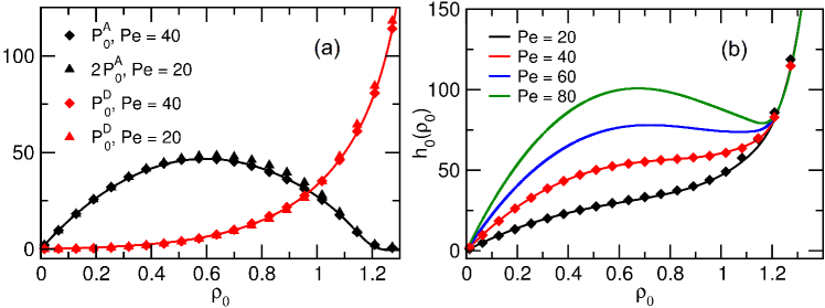
Figure 8: Construction of the equation of state for the pressure of PFAPs. (a) $P^{A}$ and $P^{D}$ (symbols) as a function of the average density $\rho_{0}$ measured in simulations of homogeneous systems ($\mathrm{Pe}<\mathrm{Pe}_{c}$). The solid lines show fits to the data at ${\rm Pe}=40$ using the functional forms $P_{0}^{A}$ and $P_{0}^{D}$ detailed in B.3. As seen from the rescaling, $P^{A}_{0}$ scales linearly with ${\rm Pe}$ while $P^{D}_{0}$ is independent of ${\rm Pe}$. We use this scaling to extrapolate the equation of state to the region where the system phase separates ($\mathrm{Pe}>\mathrm{Pe}_{c}$). (b) The full equation of state (solid lines) for the pressure $h_{0}=P_{0}^{A}+P_{0}^{D}$, with symbols denoting numerical measurements. The curves for ${\rm Pe}=60$ and ${\rm Pe}=80$ are extrapolated from measurements at ${\rm Pe}=40$ using the above scaling arguments.

Numerical strategy and results

To numerically construct the phase diagram, we first derive an approximation to the bulk equation of state $h_{0}(\rho)$. Then, we measure $h(x)$ numerically via Eq. (63) from which we subtract $h_{0}(\rho(x))$ to obtain $h_{1}$, which is integrated to obtain the numerical value of $\Delta A$. The right hand side of Eq. (69) is then held constant at this value, and the binodals are determined as the intersect between the EOS $h_{0}(\nu)$ and a horizontal line of ordinate $\bar{h}$ whose value is adjusted until it satisfies Eq. (69). Note that, for the parameter range of interest here, the two contributions to $h$ proportional to $D_{t}$ are negligible and we thus discard them hereafter.

1. We first construct an analytical approximation for the pressure $h_{0}(\rho_{0})$ by measuring the active and direct pressures from an ABP simulation in the homogeneous region (${\rm Pe}<{\rm Pe}_{\rm c}$) using Eqs. (64). Following the route proposed in [17]: we then apply scaling arguments to extrapolate the EOS into the two-phase region ${\rm Pe}>{\rm Pe}_{c}$. Fig. 8 explains and verifies the proposed scaling in the low-Péclet region and shows the resulting EOS for $P^{A}_{0}$ and $P^{D}_{0}$. Details about the numerical procedure (refined with respect to Ref. [17]) can be found in B.3.

2. The next step is to numerically determine $h_{1}$ using Eq. (67) and, through it, the value of $\Delta A$. In numerical simulations of phase-separated systems in a slab geometry (see Fig. 9a), we thus measure the profiles $\rho(x)$, $P^{A}(x)$, $P^{D}(x)$ and $\mathds{Q}_{xx}(x)$ across the interface (see Fig. 9b-c). Using the EOS $P^{A}_{0}(\rho)$ and $P^{D}_{0}(\rho)$ from (i) together with the measured density profile $\rho(x)$ we obtain the gradient contributions to the active and direct pressures as $P_{1}^{A/D}(x)=P^{A/D}(x)-P^{A/D}_{0}(\rho(x))$ (Fig. 9d). Together with $\mathds{Q}_{xx}(x)$, this directly provides $h_{1}(x)$ and hence the value of $\Delta A$ in Eq. (69).

   

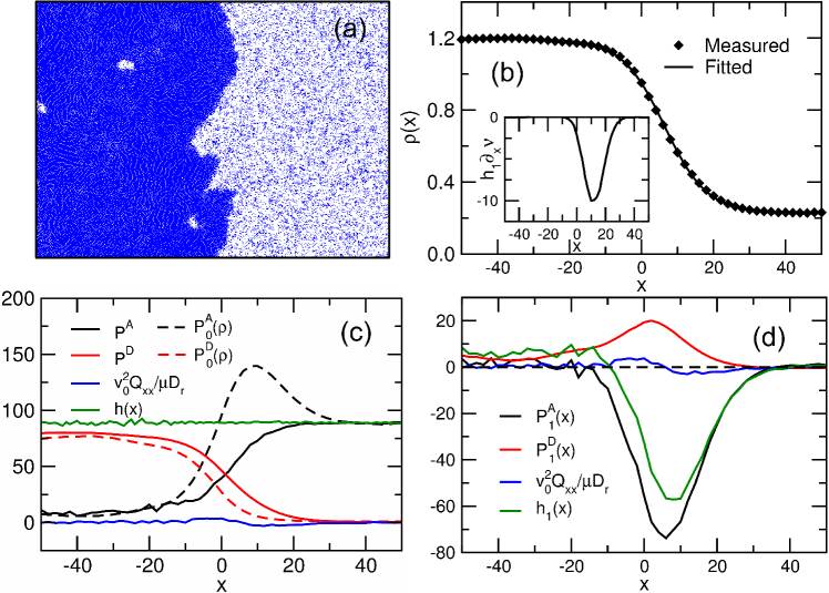
   Figure 9: (a) Close-up of a snapshot showing the interfacial region in a phase-separated system at ${\rm Pe}=120$. (b) Density field $\rho(x)$ across the interface in (a), averaged over $t$ and $y$. The solid line is a fit to a hyperbolic tangent function. Inset: Plot of $h_{1}\partial_{x}\nu$ across the interface. The area under the curve quantifies the violation $\Delta A$ of the Maxwell construction (69). (c) Profiles of the total pressure $h(x)$ and its three non-negligible components $P^{A}$, $P^{D}$ and $v_{0}^{2}\mathds{Q}_{xx}/\mu D_{r}$ (solid lines). The dashed lines correspond to the local contributions $P^{A}_{0}(\rho(x))$ and $P^{D}_{0}(\rho(x))$ that are predicted by the equation of state for a homogeneous system at density $\rho(x)$. (d) The interfacial contributions to the pressure, entering $h_{1}$ in Eq. (67).

3. Using the equation of state $h_{0}(\nu)$, we now adjust $\bar{h}$ in Eq. (69) until $\Delta A$ matches the value computed in step (ii) as shown in Fig. 10a. The resulting $\bar{h}$ and the corresponding two values of $\nu_{g}$ and $\nu_{\ell}$ constitute our prediction for the pressure at coexistence and the binodals.

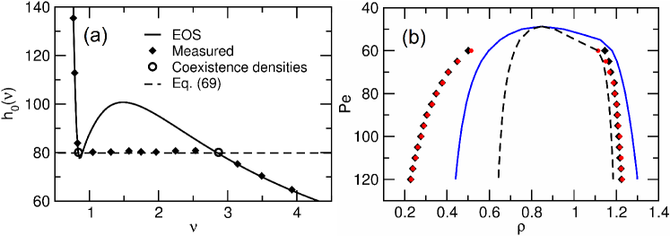
Figure 10: (a) Unequal-area construction on the equation of state $h_{0}(\nu)$ (solid lines) at Pe = 80, using the value of $\Delta A$ obtained by measuring the gradient terms. Open circles correspond to the measured binodals, and filled diamonds correspond to the pressures measured in the numerics. Note that the generalized pressure remains constant along the tie line. Dashed lines indicate pressures predicted by the unequal-area construction across the tie line. (b) Phase diagrams of PFAPs, measured numerically (diamonds), through our prediction Eq. (69) (red circles), and from the equilibrium Maxwell construction with $\Delta A=0$ (blue line). The dashed line corresponds to the boundaries of the spinodal region $h_{0}^{\prime}(\rho)<0$.

As seen in Fig. 10b, the predicted coexistence densities match very well the measured ones. We stress again that this is not a first principle prediction, since we do not use an analytic expression for the gradient terms, which thus have to be measured numerically. Nevertheless, the excellent agreement confirms the scenario proposed in Section 1 for MIPS: unlike in equilbrium, the interfacial contributions are essential in fixing the coexistence densities. Indeed, the equilibrium Maxwell construction (equivalent to taking $\Delta A=0$ in Eq. (69)) clearly fails to account for the phase diagram of PFAPs, as shown in Fig. 10b. Therefore, the interfacial contributions have to be accounted for, either by defining an effective density as in Sections 1, 1.6 and 2, or by quantifying the violation of the equilibrium constructions, as demonstrated here.

We finally note that the behavior of the interfacial terms $P^{A}_{1}$ and $P^{D}_{1}$ in Fig. 9d can be qualitatively understood as arising from the polarization of the gas-liquid interface. Since a particle at the interface is on average oriented towards the (denser) liquid phase, i.e., up the density gradient, it experiences a more efficient collisional slow-down than it would in an isotropic environment at the same local density. Since $P^{A}[\rho]$ is proportional to the effective swim-speed $v$, this will yield a lower $P^{A}$ than in the isotropic phase, and thus a negative $P_{1}^{A}$. Conversely, as $P^{D}$ is proportional to the amount of repulsive particle contacts experienced by the particle, the same argument will lead to a positive interfacial contribution $P^{D}_{1}$ to the direct pressure, confirming the observations in Fig. 9d. Since these two terms give the dominant contributions to $h_{1}$, we thus conclude that, at the microscopic level, the phase coexistence densities in PFAPs is controlled by the polar ordering of particles at the gas-liquid interface.

3.4 Finite-size corrections.

We now turn to study the finite-size corrections to the phase equilibria of PFAPs. As previously, we consider a circular droplet of radius $r_{d}$ (see Fig. 2). Following Section 1.5, the pressure jump across the interface is given at leading order in $1/r_{d}$ by

$$\Delta h_{0}=\frac{\gamma}{r_{d}};\qquad\gamma=\int_{x_{\ell}}^{x_{g}}(\sigma_{yy}-\sigma_{xx})dx,$$ (70)

where the surface tension $\gamma$ is measured across a planar interface perpendicular to $\mathbf{\hat{x}}$. We follow the same route as for QSAPs and measure independently $\Delta h_{0}$ and $\gamma$ in numerical simulations to characterize the finite-size corrections to the phase coexistence.

To understand the different contributions to $\gamma$, we introduce the difference between the $xx$ and $yy$ components for each term in the stress tensor (60) (recall that the terms proportional to $D_{t}$ are negligible):

$$\delta P_{A} = \frac{v_{0}}{\mu D_{r}}(\mathds{I}_{xx}^{(1)}-\mathds{I}_{yy}^{(1)})$$ (71)

$$\delta P_{D} = -\sigma^{\rm IK}_{xx}+\sigma^{\rm IK}_{yy}$$ (72)

$${\delta\mathds{Q}} = \mathds{Q}_{xx}-\mathds{Q}_{yy}\;.$$ (73)

The surface tension is then given by

$$\gamma=\int_{x_{\ell}}^{x_{g}}\left(\delta P_{A}+\delta P_{D}+\frac{v_{0}^{2}}{\mu D_{r}}\delta\mathds{Q}\right)dx,$$ (74)

These three contributions and their sum, $\sigma_{yy}-\sigma_{xx}$, are plotted in Fig. 11, as measured across a flat (on average) interface; the resulting integral yields the estimate $\gamma\approx-140$ in the units of our simulations. Interestingly, the contribution of the direct term $\delta P_{D}$ is completely negligible, in contrast to the equilibrium case in which the phase separation is due to attractive forces, which also determine the surface tension. Here, the main contributions stem from the anisotropy of the active pressure in the interface, as well as from the anisotropic nematic order of the particles in the interfacial region.

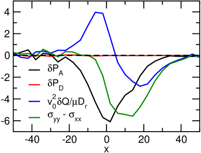
Figure 11: The three contributions to the difference between the tangential and normal stress components as defined in Eqs. (71)–(73), measured from a simulation in slab geometry at ${\rm Pe}=100$. The integral of the total stress difference $\sigma_{yy}-\sigma_{xx}$ across the interface is the effective “surface tension” $\gamma$ defined in Eq. (70).

We furthermore note that the resulting value of the surface tension is negative, which confirms the finding of Ref.[32] and can be rationalized following [42] by considering the escape angle of an active particle exiting a curved interface.

We now evaluate the effective Laplace pressure $\Delta h_{0}$ for curved droplets of different radii. Although this quantity is in principle directly measurable in simulations, it is numerically challenging due to the large fluctuations in the local pressure. We thus instead proceed similarly as for QSAPs, by first accurately measuring the coexisting densities in finite systems in which a liquid droplet of radius $r_{d}$ coexists with a vapor background. These are shown in Fig. 12a, showing that the liquid phase is effectively depleted for finite $r_{d}$, hence confirming the heuristic argument given in [42]. The correction to the coexistence densities is again found to be compatible with a $1/r_{d}$ decay. The pressure jump can then be computed using the equation of state and the measured densities as $\Delta h_{0}=h_{0}(\rho_{\ell})-h_{0}(\rho_{g})$, shown in Fig. 12b. To extract the leading order behavior in $1/r_{d}$, we fit $\Delta h_{0}(r_{d})$ with two parameters, using a function $c_{1}/r_{d}+c_{2}/r_{d}^{2}$. The second-order term is necessary because the width of the liquid-vapor interface is large ($\approx 40$, see Fig. 9b) so that the assumption of large $r_{d}$ does not hold. The leading-order coefficient from the fit in Fig. 12 corresponds to a value of $\gamma\approx-230$, to be compared to $\gamma=-140$ measured across the straight interface in Fig. 11. The sign and order of magnitude are thus correctly captured, in spite of the many approximations and numerical difficulties inherent in these measurements.

We stress that the procedure we detail above retains all the gradient terms entering $\boldsymbol{\sigma}$ through $h_{1}$, and hence accounts for the negative value of $\gamma$. As explained before, we have not, however, carried out explicitly a gradient expansion of $\boldsymbol{\sigma}$. Therefore, we do not know whether PFAPs can be quantitatively described by Eq. (16) and (17). We have shown that, in the formalism of Section 1, phase-separated solutions are compatible with a negative $\gamma$. However, the finite size corrections derived in Section 1.5 are constrained by the equality of generalized chemical potential in the two phases which imposes that the density correction $\rho-\rho_{\infty}$ take the same sign in the two phases. This is at odds with the observation of Fig. 12(a), thereby suggesting that PFAPs are not fully described by our generalized Cahn-Hilliard equation. A promising suggestion is that the finite size effects of PFAPs are best described by a more general gradient expansion which would imply the analogue of a Laplace pressure jump for the chemical potential [30].

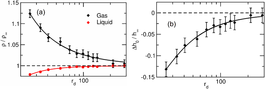
Figure 12: (a) Coexisting densities measured numerically as a function of the droplet radius for ${\rm Pe}=100$, normalized with the corresponding densities $\rho_{\infty}$ in the slab geometry (i.e., $r_{d}=\infty$). The solid lines indicate fits to the measured data using the function $\rho/\rho_{\infty}=1+c_{1}/r_{d}+c_{2}/r_{d}^{2}$, with $c_{1}$ and $c_{2}$ fitting parameters. Note that these measurements are very sensitive to the definition of coexisting densities, e.g. using the positions of the peaks of maximum probability in the distribution $P(\rho)$ of local density $\rho$ vs using the average of such peaks, so that we can expect at best semiquantitative agreement with theory. The droplet radii $r_{d}$ are estimated from the phase volumes obtained from the integral of the respective peaks in $P(\rho)$. (b) The corresponding difference in coexistence pressure $\Delta h_{0}$, obtained from the densities in (a) using the numerical EOS, and normalized with the pressure $h_{\infty}$ for a flat interface. Solid lines show fits to $\Delta h_{0}/h_{\infty}=c_{1}/r_{d}+c_{2}/r_{d}^{2}$, where the fitting parameter $c_{1}h_{\infty}\approx-230$ is an estimation for the surface tension $\gamma$.

4 Change of ensembles

One powerful aspect of equilibrium thermodynamics is that it relates the physical states of a system under different environmental constraints. Beyond its engineering value, the existence of several ensembles provides useful theoretical tools to study phase transitions [43]. Similar developments for non-equilibrium systems have however proven difficult [44, 45, 46]. Interestingly, our formalism allows some progress.

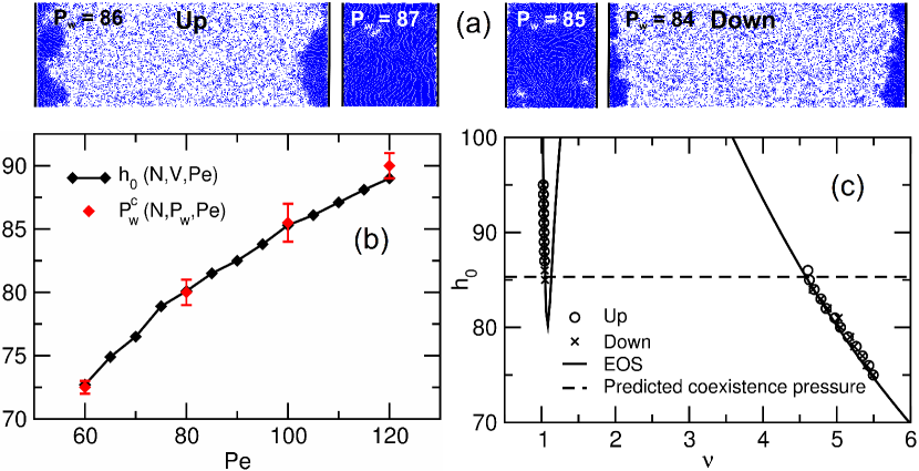
Figure 13: PFAPs in the isobaric $N,P_{w},{\rm Pe}$ ensemble. (a): Snapshots from PFAP simulations with a mobile wall imposing a pressure $P_{w}$ at ${\rm Pe}=100$ during a slow upwards (left) and downwards (right) pressure ramp (for movies, see [47]). In the isobaric ensemble, the phase transition becomes discontinuous, in contrast to the phase coexistence observed in constant-volume simulations. (b): For each Péclet number, the discontinuous phase transition (red symbols) occurs when the imposed pressure $P_{w}^{c}$ equals the mechanical pressure of coexisting gas and liquids in the isochoric ensemble (black symbols). (c): When ramping the imposed pressure slowly up or down across the transition, the measured phase densities (symbols) fall on the pressure equation of state (solid black line), with a small hysteresis loop centered around the coexistence pressure (horizontal dashed line).

We adapt our previous constant volume (isochoric) simulations to consider an isobaric (constant pressure) ensemble. PFAPs or QSAPs are now confined by mobile harmonic walls, subject to a constant force density $P_{w}$ which imposes a mechanical pressure $P=P_{w}$ (see Fig. 13a and movies in [47]). Since $P=h_{0}$ is a generalized thermodynamic variable for PFAPs, we expect, as in equilibrium, that the coexistence region of the isochoric ($N,V,{\rm Pe}$) ensemble collapses onto a coexistence line in the isobaric ($N,P,{\rm Pe}$) case, corresponding to the pressure at coexistence in the isochoric ensemble (see Fig 13b). Inposed-pressure loops carried out by slowly ramping up and down $P_{w}$ then lead to small hysteresis loops around the value of $P_{w}$ corresponding to coexistence. These loops would vanish in the large system size limit for quasi-static ramping of $P_{w}$ (see Fig 13c).

In contrast, for QSAPs the mechanical pressure $P$ is unrelated to either of the generalized variables $g_{0},h_{0}$. The same value of $P_{w}$ may thus lead to different states of the system depending on its history: the Gibbs phase rule does not apply for QSAPs in this ensemble. This translates into large hysteresis loops when slowly cycling $P_{w}$, as shown in Fig 14.

On a fundamental level, the different relationship between thermodynamical and mechanical observables can be related to the presence or absence of an effective momentum conservation in the steady state [48]. From a more practical point of view, this can be traced back to the fact that adding an external potential $U$ to PFAPs gives a simple force balance equation in a flux-free steady state

$$\rho{\nabla U}=\nabla\cdot\boldsymbol{\sigma}.$$ (75)

This makes the mechanical pressure a state variable for PFAPs while the more complicated relationship between $g_{0},h_{0}$ and $U$ for QSAPs breaks this link [1]. This explains the different roles of pressure in these two systems when considering change of ensembles.

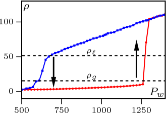
Figure 14: For QSAPs, the volume (or here the density at fixed particle number $N=150000$) is not single-valued in the imposed mechanical pressure $P_{w}$, leading to large hysteresis loops. Note that the mechanical pressures $P_{w}$ corresponding to liquid and gas binodals are different, as expected. Parameters: $\rho_{m}=25$, $v_{0}=20$, $v_{1}=5$, $\tau=1$, vertical size $L_{y}=50$.

5 Conclusion

In this article, we have shown how to derive the phase equilibria of MIPS for a number of different systems. At the hydrodynamic scale, the simple gradient terms that drive Active Model B [11] out of equilibrium still allow for the construction of a generalized thermodynamics, which leads to the definition of generalized chemical potential, pressure and surface tension. Using this formalism, we account quantitatively for the binodal curve of fully-phase separated systems as well as for its finite-size corrections.

For quorum-sensing active particles, we have shown how to build a hydrodynamic description that fits within our generalized thermodynamic framework, using a combination of a local mean-field approximation and a gradient expansion. Despite these approximations, our formalism accounts quantitatively for the phase diagram of QSAPs. For particles interacting via repulsive pairwise forces, no closed hydrodynamics description including the relevant gradient terms exist in the literature. We thus followed an alternative route and showed how the binodals are selected by an equality of mechanical pressure complemented by a violation of the equilibrium Maxwell construction due to interfacial contributions.

Our identification of the relevant intensive variables governing the phase equilibrium of MIPS is important to define thermodynamic ensembles, which we have illustrated by considering the isobaric ensemble for QSAPs and PFAPs. We hope that our approach will pave the way towards a more general definition of intensive thermodynamic parameters [44, 45, 46] for active systems. Building a thermodynamic of active matter would further improve our understanding and control of these intriguing systems and has become a central question in the field [1, 49, 12, 37, 13, 11, 35, 17, 50, 51, 25, 32, 52, 53, 54, 20].

Acknowledgments: APS and JS contributed equally to this work. We thank M. Kardar and H. Touchette for discussions. APS acknowledges funding through a PLS fellowship from the Gordon and Betty Moore foundation. JS is funded by a Project Grant from the Swedish Research Council (2015-05449). JT & AS ackownledge the hospitality of MLB Center for Theoretical Physics. MEC is funded by the Royal Society. This work was funded in part by EPSRC Grant EP/J007404. YK is supported by an I-CORE Program of the Planning and Budgeting Committee of the Israel Science Foundation and an Israel Science Foundation grant. JT is funded by ANR Baccterns. JT & YK acknowledge support from a joint CNRS-MOST grant. The PFAP simulations were performed on resources provided by the Swedish National Infrastructure for Computing (SNIC) at LUNARC.

Appendix A Hydrodynamics of QSAPs

In this section we derive the hydrodynamic equations of QSAPs interacting via a density-dependent velocity. In the hydrodynamic description, we consider only smooth density profiles, slowly varying in space and time, so that we can expand the self-propulsion speed as

$$v[\tilde{\rho}(\mathbf{r}_{i}+\varepsilon\mathbf{u}_{i})]\simeq v[\tilde{\rho}(\mathbf{r}_{i})]+\varepsilon\mathbf{u}_{i}\cdot\nabla v[\tilde{\rho}(\mathbf{r}_{i})]$$ (76)

Furthermore, for a system of size $L$, the (diffusive) relaxation time $\tau_{D}$ of the density profile scales as $L^{2}$ and is much larger than the microscopic orientational persistence time $\tau=(\alpha+(d-1)D_{r})^{-1}$. To construct the large-scale dynamics of QSAPs, we first coarse-grain their dynamics on time scales such that $\tau\ll t\ll\tau_{D}\sim L^{2}$, following the method detailed in [24, 35]. In practice, we first construct a diffusive approximation to the dynamics of QSAPs on a time scale over which their density field does not relax so that the propulsion velocity of a single particle depends on its position and orientation through a function $v(\mathbf{r}_{i},\mathbf{u}_{i})$ which is constant in time.

A.1 Diffusion-drift approximation

The probability $\psi(\mathbf{r},\mathbf{u})$ of finding a given particle at position $\mathbf{r}$ with an orientation $\mathbf{u}$ evolves according to:

$$\dot{\psi}=-\nabla\cdot\left[v(\mathbf{r},\mathbf{u})\mathbf{u}\psi-D_{t}\nabla\psi\right]+D_{r}\Delta_{u}\psi-\alpha\psi+\frac{\alpha}{\Omega}\int d\Omega^{\prime}\psi$$ (77)

$\psi$ can be expanded in spherical (3d) or Fourier (2d) harmonics:

$$\psi(\mathbf{r},\mathbf{u})=\varphi+\mathbf{p}\cdot\mathbf{u}+Q:M+\Theta[\psi]$$ (78)

where $M_{ab}=u_{a}u_{b}-\delta_{ab}/d$, and $\varphi$, $\mathbf{p}$, and $Q$ solely depend on $\mathbf{r}$. $\Theta[\psi]$ is the projection of $\psi$ on higher order harmonics, which plays no role in the following. We furthermore introduce the scalar product

$$\langle f,\,g\rangle=\int d\mathbf{u}f(\mathbf{u})g(\mathbf{u})$$ (79)

where the integration is over the unit sphere. The components of $\psi$ in the expansion (78) are then obtained from

$$\langle 1,\,\psi\rangle=\Omega\varphi;\qquad\langle\mathbf{u},\psi\rangle=\frac{\Omega}{d}\mathbf{p};\qquad\langle M_{ab},\psi\rangle=\tilde{\Omega}Q_{ab}$$ (80)

where $\Omega$ is the area of the unit sphere and $\tilde{\Omega}\equiv\frac{2\Omega}{d(d+2)}$. Projecting Eq. (77) onto 1, $\mathbf{u}$ and $M$ yields the dynamics of $\varphi$, $\mathbf{p}$ and $Q$:

$$\dot{\varphi} = -\big{\langle}\frac{1}{\Omega},\nabla\cdot v\mathbf{u}\psi\big{\rangle}+\nabla\cdot(D_{t}\nabla\varphi)$$ (81)

$$\dot{\mathbf{p}} = -\big{\langle}\frac{d\mathbf{u}}{\Omega},\nabla\cdot v\mathbf{u}\psi\big{\rangle}+\nabla\cdot(D_{t}\nabla\mathbf{p})-\frac{\mathbf{p}}{\tau}$$ (82)

$$\dot{Q} = -\big{\langle}\frac{M}{\tilde{\Omega}},\nabla\cdot v\mathbf{u}\psi\big{\rangle}+\nabla\cdot(D_{t}\nabla Q)-\frac{Q}{\tau_{Q}}$$ (83)

where $\tau_{Q}^{-1}=2dD_{r}+\alpha$ is the relaxation time of the second harmonic $Q$. Similar equations could also be derived for higher order harmonics. However, the structure of Eqs. (81-83) immediately shows that $\varphi$ is the sole hydrodynamic field since all higher order harmonics relax on times of order ${\cal O}(1)$ ($\tau$ for $\mathbf{p}$ and $\tau_{Q}$ for $Q$). Consequently, one can assume that $\dot{\mathbf{p}}$ and $\dot{Q}$ vanish, as would the time derivative of higher order harmonics. The structure of Eqs. (82-83) then shows that all harmonics beyond $\varphi$ are at least of order ${\cal O}(\nabla)$ in the gradient expansion.

Going further than Refs. [24, 35], we now also expand $v$ in spherical harmonics. Under (76), only the first two harmonics matter and we use:

$$v(\mathbf{r},\mathbf{u})\equiv v^{0}(\mathbf{r})+\mathbf{v}^{1}(\mathbf{r})\cdot\mathbf{u}$$ (84)

where $\mathbf{v}^{1}$ will be of order ${\cal O}(\nabla)$ in the gradient expansion. Eq. (83) then gives for $Q$:

$$\dot{Q}_{ab} = -\frac{d+2}{2}\left(\partial_{c}(v^{0}p_{d}+v^{1}_{d}\varphi)B_{abcd}+\partial_{c}v^{1}_{d}Q_{ef}C_{abcdef}\right)$$ (85)

$$\qquad+\partial_{c}D_{t}\partial_{c}Q_{ab}-\tau_{Q}^{-1}Q_{ab}+\partial_{c}\chi^{Q}_{abc}$$

where the constant tensors $B$ and $C$ are defined as

$$B_{abcd}\equiv\frac{d}{\Omega}\langle M_{ab},M_{cd}\rangle,\quad C_{abcdef}\equiv\frac{d}{\Omega}\langle M_{ab},u_{c}u_{d}M_{ef}\rangle$$

and $\chi_{abc}^{Q}\equiv\langle M_{ab},u_{c}v\Theta[\psi]\rangle/\tilde{\Omega}$ stems from higher order harmonics. Since $\dot{Q}\simeq 0$ on hydrodynamic time and space scales, one finds at first order in gradients

$$Q_{ab}\simeq O(\nabla^{2})$$ (86)

Similarly, the dynamics of $\dot{p}$ is given by

$$\dot{p}_{a} = -\partial_{a}v^{0}\varphi-\frac{2}{d+2}\partial_{b}v^{0}Q_{ab}+\frac{1}{d+2}(\partial_{b}v^{1}_{b}p_{a}$$

$$\;+\partial_{b}v^{1}_{a}p_{b}+\partial_{a}v^{1}_{b}p_{b})+\partial_{b}D_{t}\partial_{b}p_{a}-\tau p_{a}+\partial_{b}\chi_{ab}^{p}$$

where $\chi_{ab}^{p}=d\langle u_{a},u_{b}v\Theta[\psi]\rangle/\Omega$. Again, using $\dot{\mathbf{p}}\simeq 0$, one finds at first order in gradients

$$p_{a}=-\tau\partial_{a}v^{0}\varphi+O(\nabla^{2})$$ (88)

Finally, the dynamics of $\varphi$ reads

$$\dot{\varphi}=-\frac{1}{d}\partial_{a}(v^{0}p_{a}+v^{1}_{a}\varphi)-\frac{2}{d(d+2)}\partial_{a}v^{1}_{b}Q_{ab}+D_{t}\partial_{a}^{2}\varphi.$$ (89)

Using Eq. (88) and $Q_{ab}=O(\nabla^{2})$, the dynamics of $\varphi$ at diffusion-drift level reduces to the Fokker-Planck equation

$$\dot{\varphi}=-\nabla\cdot\left[\mathbf{V}\varphi-D\nabla\varphi\right]$$ (90)

with

$$\mathbf{V}=\frac{\varepsilon\nabla v}{d}-\frac{\tau v\nabla v}{d};\qquad D=D_{t}+\frac{\tau v^{2}}{d}$$ (91)

A.2 Hydrodynamic equation

The Fokker-Planck equation (90) for $\varphi$ is equivalent to an Itō-Langevin dynamics for the position of the QSAP. From there, one can derive the collective dynamics of $N$ QSAPs using Itō calculus, as was done many times in simpler settings [55, 1, 35]. For simplicity, we consider here the case $D_{t}=0$. One then finds the coarse-grained $N$-body density of QSAPs to follow the stochastic dynamics

$$\dot{\rho}=\nabla\cdot\Big{[}\rho D(\tilde{\rho})\nabla\big{[}\log\rho v(\tilde{\rho})+\frac{\varepsilon}{\tau v(\tilde{\rho})}\big{]}+\sqrt{2\rho D(\tilde{\rho})}\boldsymbol{\eta}\Big{]},\\$$ (92)

We can now expand $\tilde{\rho}(\mathbf{r})$ in gradients of the density field

$$\tilde{\rho}\simeq\rho+\frac{1}{2}\ell^{2}\Delta\rho+{\cal O}(\nabla^{3})$$ (93)

with $\ell^{2}=\int r^{2}K(\mathbf{r})d\mathbf{r}$. In turn, this implies for the propulsion speed

$$v[\tilde{\rho}(\mathbf{r})]\simeq v(\rho)+\ell^{2}v^{\prime}(\rho)\Delta\rho+{\cal O}(\nabla^{3})$$ (94)

Finally one finds the self-consistent dynamics for $\rho$:

$$\dot{\rho}=\nabla\cdot\left[\rho D(\tilde{\rho})\nabla\left(\frac{\delta\mathcal{F}}{\delta\rho}-\kappa(\rho)\Delta\rho\right)+\sqrt{2\rho D(\tilde{\rho})}\boldsymbol{\eta}\right],\\$$ (95)

where ${\cal F}[\rho]=\int d\mathbf{r}f[\rho(\mathbf{r})]$ and

$$f^{\prime}(\rho)=\log[\rho v(\rho)]+\frac{\varepsilon}{\tau v(\rho)};\,\,\kappa(\rho)=-\ell^{2}\frac{v^{\prime}(\rho)}{v(\rho)}\left(1-\frac{\varepsilon}{\tau v(\rho)}\right)$$ (96)

As hinted before [1, 11, 35], the non-locality of the density sampling results in a ‘surface tension generating’ term $\kappa(\rho)$. Interestingly, the asymmetric sensing $\varepsilon$ affects both the free energy density $f(\rho)$ and the gradient terms $\kappa(\rho)$.

Appendix B PFAPs

B.1 Constant-volume simulations

Simulations in the isochoric (constant-volume) ensemble were carried out in rectangular boxes of size $L_{x}\times L_{y}$ with periodic boundary conditions using a modified version of the LAMMPS molecular dynamics package[56]. For simulations in slab geometry at coexistence, we chose $L_{x}=500$, $L_{y}=300$, and $N=$ 115,000 particles. In order to ensure a stable, flat (on average) interface spanning the $\hat{\mathbf{y}}$-direction, these simulations were initiated by first equilibrating the particles in a smaller box of size $300\times 300$ with $v_{0}=0$, yielding a near-close-packed phase. After this initial equilibration, the box was expanded in the $\hat{\mathbf{x}}$-direction and the activity was turned on, after which the system relaxed towards a phase-separated steady state. The simulations were run for a time $t=1000$, the data being collected over the second half of this time.

We compute binodal densities by coarse-graining the local density using a weighting function $w(r)\propto\exp[-r^{2}_{\mathrm{cut}}/(r^{2}_{\mathrm{cut}}-r^{2})]$, where $r$ is the distance between the particle and the measuring point, and $r_{\mathrm{cut}}$ is a cut-off distance. Histograms of the density then show two peaks that we identify as the coexisting densities.

In order to handle the relatively large fluctuations in the position of the interface, the density and pressure profiles measured on each timestep was translated to a common origin. This point was taken to be the point where the density (averaged over $y$) has fallen below $\rho=0.95$.

B.2 Constant-pressure simulations

Here, we used a simulation box with $L_{y}=100$, $N=10000$ and periodic boundary conditions in the vertical direction only. In the $x$-direction, the system was confined by two walls modeled by harmonic potentials:

$$V_{w}^{R}(x) = k(x-x_{R})^{2}\Theta(x-x_{R})$$ (97)

$$V_{w}^{L}(x) = k(x-x_{L})^{2}\Theta(x_{L}-x)$$ (98)

where $k$ controls the stiffness of the walls (we take $k=5$). The right wall is fixed at $x=x_{R}$, while the position $x_{L}$ of the left wall obeys the deterministic overdamped dynamics:

$$\dot{x}_{L}=\gamma\Big{(}P_{w}L_{y}-\sum_{i=1}^{N}\frac{\partial V^{\ell}_{w}}{\partial x_{i}}\Big{)}$$ (99)

where $x_{i}$ is the abscissa of particle $i$, $P_{w}$ the pressure externally imposed on the wall and $\gamma$ its mobility, taken to be $\gamma=0.1$. The dynamics is integrated by Euler time stepping, with the same time step as for the particles. To compute the phase diagram in the isobaric ($N,P_{w},{\rm Pe}$) ensemble, we ramp $P_{w}$ up and down very slowly. For each ${\rm Pe}$, the system was first equilibrated at a starting pressure $P_{w}$, which was then incremented or decremented in steps of $\pm 1$ every $10^{8}$ time steps.

B.3 Construction of the equation of state

In order to separate the gradient contributions from the bulk contributions to $P_{A}$ and $P_{D}$, one needs an accurate EOS for the full phase-separated parameter region – something which is not known a priori. In order to obtain an approximate EOS, we adopt a refined version of the strategy followed in [17]: we (i) measure $P^{0}_{A}(\rho)$ and $P^{0}_{D}(\rho)$ for $\mathrm{Pe}<\mathrm{Pe}_{c}$, where homogeneous systems are stable for all densities, and (ii) apply scaling arguments to extend the validity of the EOS to $\mathrm{Pe}>\mathrm{Pe}_{c}$.

We start from the exact expression of the active pressure in a homogeneous system [17]

$$\mu P^{0}_{A}(\rho)=\frac{v_{0}}{2D_{r}}v(\rho)\rho,$$ (100)

where $v(\rho)$ is the density-dependent single-particle swim velocity projected along its orientation [17]

$$v(\rho)\equiv v_{0}+2\mathds{I}_{xx}/\rho=v_{0}+\langle\mathbf{u}(\theta_{i})\!\cdot\!\sum_{j\neq i}\mathbf{F}(\mathbf{r}_{j}-\mathbf{r}_{i})\rangle=\langle\dot{\bf r}_{i}\cdot{\bf u}_{i}\rangle\;.$$ (101)

As has been shown several times before [3, 7, 6, 29, 17], $v(\rho)$ is accurately described by a linearly decreasing function up to near-close-packed densities. However, as the details of the high-density region of the EOS are very important for the accuracy of the predicted binodals, we furthermore include a quadratic term in $\rho$ and a switching function which ensures a smooth transition to $v\rightarrow 0$:

$$v(\rho)=\frac{v_{0}}{2}(1-s_{1}\rho+s_{2}\rho^{2})(1-\tanh(s_{3}(\rho-s_{4}))),$$ (102)

where $s_{1}-s_{4}$ are fitting parameters which are found to be essentially independent of $D_{r}$ (see Fig. 8) as long as we remain in the ${\rm Pe}<{\rm Pe}_{c}$ region. The local EOS for $P_{A}^{0}$ is then given by (100) with (102).

We now consider the local EOS for the direct pressure. For the values of $v_{0}$ and $\epsilon$ used in this study, which control the effective stiffness of the WCA potential, $P_{D}$ is found to be independent of $D_{r}$ (see Fig. 8). For Pe= 40, we find that $P^{0}_{D}(\rho)$ is accurately fitted by a biexponential function:

$$P^{0}_{D}(\rho)=d_{1}\left(\exp(d_{2}\rho)-1\right)+d_{3}\left(\exp(d_{4}\rho)-1\right),$$ (103)

where $d_{1}-d_{4}$ are fitting parameters.

References

- [1] Tailleur J and Cates M 2008 Phys. Rev. Lett. 100 218103
- [2] Thompson A, Tailleur J, Cates M and Blythe R 2011 J. Stat. Mech. Theory Exp. 2011 P02029
- [3] Fily Y and Marchetti M C 2012 Phys. Rev. Lett. 108 235702
- [4] Redner G S, Hagan M F and Baskaran A 2013 Phys. Rev. Lett. 110 055701
- [5] Bialké J, Löwen H and Speck T 2013 EPL 103 30008
- [6] Stenhammar J, Tiribocchi A, Allen R J, Marenduzzo D and Cates M E 2013 Phys. Rev. Lett. 111 145702
- [7] Buttinoni I, Bialké J, Kümmel F, Löwen H, Bechinger C and Speck T 2013 Phys. Rev. Lett. 110 238301
- [8] Wysocki A, Winkler R G and Gompper G 2014 EPL 105 48004
- [9] Theurkauff I, Cottin-Bizonne C, Palacci J, Ybert C and Bocquet L 2012 Phys. Rev. Lett. 108 268303
- [10] Soto R and Golestanian R 2014 Phys. Rev. E 89 012706
- [11] Wittkowski R, Tiribocchi A, Stenhammar J, Allen R J, Marenduzzo D and Cates M E 2014 Nat. Commun. 5 4351
- [12] Takatori S C, Yan W and Brady J F 2014 Phys. Rev. Lett. 113 028103
- [13] Speck T, Bialké J, Menzel A M and Löwen H 2014 Phys. Rev. Lett. 112 218304
- [14] Matas-Navarro R, Golestanian R, Liverpool T B and Fielding S M 2014 Phys. Rev. E 90 032304
- [15] Zöttl A and Stark H 2014 Phys. Rev. Lett. 112 118101
- [16] Suma A, Gonnella G, Marenduzzo D and Orlandini E 2014 EPL 108 56004
- [17] Solon A P, Stenhammar J, Wittkowski R, Kardar M, Kafri Y, Cates M E and Tailleur J 2015 Phys. Rev. Lett. 114 198301
- [18] Cates M E and Tailleur J 2015 Annu. Rev. Condens. Matter Phys. 6 219–244
- [19] Redner G S, Wagner C G, Baskaran A and Hagan M F 2016 Phys. Rev. Lett. 117 148002
- [20] Paliwal S, Rodenburg J, van Roij R and Dijkstra M 2018 New. J. Phys. 20 015003
- [21] Whitelam S, Klymko K and Mandal D 2017 arXiv:1709.03951
- [22] Liu C, Fu X, Liu L, Ren X, Chau C K, Li S, Xiang L, Zeng H, Chen G, Tang L H et al. 2011 Science 334 238–241
- [23] Liu G, Patch A, Bahar F, Yllanes D, Welch R D, Marchetti M C, Thutupalli S and Shaevitz J W 2017 arXiv:1709.06012
- [24] Cates M E and Tailleur J 2013 EPL 101 20010
- [25] Takatori S C and Brady J F 2015 Phys. Rev. E 91 032117
- [26] Solon A P, Stenhammar J, Cates M E, Kafri Y and Tailleur J 2018 Phys. Rev. E 97 020602(R)
- [27] Cahn J W and Hilliard J E 1958 The Journal of chemical physics 28 258–267
- [28] Bray A J 2002 Adv. Phys. 51 481–587
- [29] Stenhammar J, Marenduzzo D, Allen R J and Cates M E 2014 Soft Matter 10 1489–1499
- [30] Tjhung E, Nardini C and Cates M E 2018 arXiv:1801.07687
- [31] Krüger M, Solon A, Démery V, Rohwer C M and Dean D S 2017 arXiv:1712.05160
- [32] Bialké J, Siebert J T, Löwen H and Speck T 2015 Phys. Rev. Lett. 115 098301
- [33] Chen Q S, Patelli A, Chaté H, Ma Y Q and Shi X Q 2017 Phys. Rev. E 96 020601
- [34] Kipnis C and Landim C 2013 Scaling limits of interacting particle systems vol 320 (Springer Science & Business Media)
- [35] Solon A, Cates M and Tailleur J 2015 Eur. Phys. J. Spec. Top. 224 1231–1262
- [36] Mijalkov M, McDaniel A, Wehr J and Volpe G 2016 Phys. Rev. X 6 011008
- [37] Yang X, Manning M L and Marchetti M C 2014 Soft Matter 10 6477–6484
- [38] Levis D, Codina J and Pagonabarraga I 2017 Soft Matter 13 8113–8119
- [39] Levis D and Berthier L 2014 Phys. Rev. E 89 062301
- [40] Farrell F, Marchetti M, Marenduzzo D and Tailleur J 2012 Phys. Rev. Lett. 108 248101
- [41] Irving J and Kirkwood J G 1950 J. Chem. Phys. 18 817–829
- [42] Lee C F 2017 Soft Matter 13 376–385
- [43] Binder K 1987 Rep. Prog. Phys. 50 783
- [44] Bertin E, Dauchot O and Droz M 2006 Phys. Rev. Lett. 96 120601
- [45] Bertin E, Martens K, Dauchot O and Droz M 2007 Phys. Rev. E 75 031120
- [46] Dickman R 2016 New. J. Phys. 18 043034
- [47] See Supplemental Material at [URL to be inserted by editor] for movies showing PFAP simulations in the isobaric ensemble.
- [48] Fily Y, Kafri Y, Solon A, Tailleur J and Turner A 2017 J. Phys. A: Math. Theor. 51 044003
- [49] Palacci J, Cottin-Bizonne C, Ybert C and Bocquet L 2010 Phys. Rev. Lett. 105 088304
- [50] Solon A P, Fily Y, Baskaran A, Cates M, Kafri Y, Kardar M and Tailleur J 2015 Nat. Phys. 11 673–678
- [51] Ginot F, Theurkauff I, Levis D, Ybert C, Bocquet L, Berthier L and Cottin-Bizonne C 2015 Phys. Rev. X 5 011004
- [52] Farage T F, Krinninger P and Brader J M 2015 Phys. Rev. E 91 042310
- [53] Marconi U M B and Maggi C 2015 Soft Matter 11 8768–8781
- [54] Fodor E, Nardini C, Cates M E, Tailleur J, Visco P and van Wijland F 2016 Phys. Rev. Lett. 117 038103
- [55] Dean D S 1996 J. Phys. A: Math. Gen. 29 L613
- [56] Plimpton S 1995 J. Comp. Phys. 117 1–19