Rotor Spectra and Berry Phases in the
Chiral Limit of QCD on a Torus

Abstract

We consider the finite-volume spectra of QCD in the chiral limit of massless up and down quarks and massive strange quarks in the baryon number sectors $B=0$ and $B=1$ for different values of the isospin. Spontaneous symmetry breaking gives rise to rotor spectra, as the chiral order parameter precesses through the vacuum manifold. Baryons of different isospin influence the motion of the order parameter through non-trivial Berry phases and associated abstract monopole fields. Our investigation provides detailed insights into the dynamics of spontaneous chiral symmetry breaking in QCD on a torus. It also sheds new light on Berry phases in the context of quantum field theory. Interestingly, the Berry gauge field resulting from QCD solves a Yang-Mills-Chern-Simons equation of motion on the vacuum manifold $SU(2)=S^{3}$.

1 Introduction

Nowadays lattice QCD calculations are performed close to the physical point, i.e. with realistic quark masses. Very interesting effects also arise in the chiral limit of exactly massless up and down quarks, where lattice QCD doesn’t work so efficiently. In this paper, we focus our theoretical study on this somewhat academic limit in order to gain a deeper understanding of the dynamics of spontaneous chiral symmetry breaking in a finite volume. In the absence of any explicit breaking of chiral symmetry, in the infinite volume QCD has infinitely many degenerate vacuum states, among which one is selected spontaneously. In a finite volume, on the other hand, all vacuum states coexist, but they are no longer exactly degenerate. Instead their energies split into a rotor spectrum with energy differences that are inversely proportional to the spatial volume. The rotor spectrum in the vacuum sector of QCD in the chiral limit was first derived by Leutwyler in [1]. The dynamics of the chiral order parameter then reduces to the quantum mechanical motion of a rotor in the vacuum manifold. The rotor spectrum in the baryon number $B=1$ and isospin $I=\frac{1}{2}$ sector has been investigated in [2]. The presence of a nucleon influences the precession of the chiral order parameter and leaves an imprint on the corresponding rotor spectrum. This manifests itself by a non-Abelian Berry phase and an abstract monopole field in the vacuum manifold. In this way, the Berry phase [3, 4], which is familiar from quantum mechanics, arises even in the context of QCD. It should be noted that the nucleon mass, which originates from spontaneous chiral symmetry breaking, remains non-zero in the chiral limit in a finite volume. This is the case even when all vacuum states are sampled by the precessing order parameter, such that, at least in a naive sense, chiral symmetry is no longer spontaneously broken. In this paper, we extend the previous studies to baryon sectors with general isospin $I$. Again, non-trivial Berry phases and monopole fields explain the resulting rotor spectra.

Similar situations also arise in $(2+1)$-d antiferromagnets of finite volume with a spontaneously broken $SU(2)_{s}$ spin symmetry. Considering a quadratic periodic volume, the quantum mechanical rotor spectrum of the precessing staggered magnetization order parameter was first calculated by Hasenfratz and Niedermayer in [5]. While the analog of the Goldstone pions in QCD are massless spinwaves (or magnons) in an antiferromagnet, the condensed matter analog of protons and neutrons are holes or electrons doped into an antiferromagnet. In this case, again Berry phases and corresponding monopole fields describe how a doped hole or electron influences the rotor spectrum associated with the precessing staggered magnetization [2]. Interestingly, the Berry gauge field that arises in this case is the same as the one associated with the rotation of diatomic molecules [6, 7, 8]. In this paper, we concentrate entirely on QCD, and leave the investigation of condensed matter analogs for future study.

In QCD we encounter a Berry gauge field that is defined on the group manifold of the $SU(2)$ flavor group. Remarkably, while the Berry gauge field is just a geometric object, it turns out to be a classical solution of a Yang-Mills-Chern-Simons equation of motion. The covariantly conserved Chern-Simons current then provides a source for the non-Abelian Berry field strength. This is similar to the problem addressed in [9]. In that case, the Berry gauge field corresponds to a Bogomolnyi-Prasad-Sommerfield (BPS) monopole solution of a Yang-Mills-Higgs equation of motion. There an adjoint Higgs field, which plays the role of a “Berry matter field”, gives rise to a conserved current.

The rest of this paper is organized as follows. Section 2 summarizes baryon chiral perturbation theory for non-relativistic baryons. In order to make the paper self-contained, Sections 3 and 4 summarize the derivation of the rotor spectrum in the vacuum (i.e. for baryon number $B=0$) and in the nucleon sector (with $B=1$ and isospin $I=\frac{1}{2}$), respectively. We also provide further details that go beyond the presentation in [2]. Section 5 provides the major new results of this work, by addressing baryon sectors of general isospin. In Section 6 we investigate the nature of the Berry gauge field, in particular, as a solution of a classical Yang-Mills-Chern-Simons equation of motion on the $SU(2)$ group manifold. Finally, Section 7 contains our conclusions.

2 Baryon Chiral Perturbation Theory

In this section we review baryon chiral perturbation theory for non-relativistic baryons [11, 12, 13, 14], which is an appropriate tool to address the low-energy physics of the precessing chiral order parameter in the presence of a baryon. We consider the chiral limit of massless up and down quarks ($m_{u}=m_{d}=0$), but we treat the strange quark as massive ($m_{s}\neq 0$). The chiral symmetry group of QCD then is $G=SU(2)_{L}\times SU(2)_{R}\times U(1)_{B}$, which is spontaneously broken to the subgroup $H=SU(2)_{L=R}\times U(1)_{B}$, where $SU(2)_{L=R}$ and $U(1)_{B}$ are the unbroken isospin and baryon number symmetries, respectively. As a consequence of chiral symmetry breaking, there are three massless Goldstone pion fields $\pi^{a}(x)$ which are described by

$$U(x)=\exp[i\pi^{a}(x)\tau_{a}/F_{\pi}]\in G/H=SU(2)\ ,$$ (2.1)

where $x=(\vec{x},t)$ is a point in Euclidean space-time, $F_{\pi}$ is the pion decay constant, and the Pauli matrices $\tau_{a}$ are the generators of $SU(2)$. The spatial zero-mode of $U(x)$ describes the orientation of the chiral order parameter in the vacuum manifold $SU(2)$, while non-zero modes correspond to pion excitations.

Under global chiral rotations, the field $U(x)$ transforms as

$$U(x)^{\prime}=LU(x)R^{\dagger}\ ,\quad L\in SU(2)_{L}\ ,\ R\in SU(2)_{R}\ ,$$ (2.2)

while under charge conjugation $C$ and parity $P$ it transforms as

$${}^{C}U(x)=U(x)^{\sf T}\ ,\quad^{P}U(\vec{x},t)=U(-\vec{x},t)^{\dagger}\ .$$ (2.3)

In order to couple the chiral order parameter field $U(x)$ to baryon fields, we first introduce the field $u(x)=U(x)^{1/2}\in SU(2)$. In order to fix the sign ambiguity of the square-root, it is important to take $U(x)^{1/2}$ at the midpoint of the shortest geodesic in the $SU(2)$ group manifold that connects $U(x)$ with the unit-element ${{\mathbbm{1}}}$ [15]. Next, we use $u(x)$ to construct a non-Abelian $SU(2)$ gauge field $v_{\mu}(x)$ and a “charged” axial-vector field $a_{\mu}(x)$ as

$$v_{\mu}(x)=\frac{1}{2}[u(x)^{\dagger}\partial_{\mu}u(x)+u(x)\partial_{\mu}u(x)^{\dagger}]=iv_{\mu}^{a}(x)\tau_{a}\ ,$$

$$a_{\mu}(x)=\frac{i}{2}[u(x)^{\dagger}\partial_{\mu}u(x)-u(x)\partial_{\mu}u(x)^{\dagger}]=a_{\mu}^{a}(x)\tau_{a}\ .$$ (2.4)

Under chiral rotations these fields transforms as

$$u(x)^{\prime}=Lu(x)V(x)^{\dagger}=V(x)u(x)R^{\dagger}\ ,$$

$$v_{\mu}(x)^{\prime}=V(x)[v_{\mu}(x)+\partial_{\mu}]V(x)^{\dagger}\ ,$$

$$a_{\mu}(x)^{\prime}=V(x)a_{\mu}(x)V(x)^{\dagger}\ .$$ (2.5)

Interestingly, the global chiral rotations $L$ and $R$ give rise to the local transformation

$$V(x)=R[R^{\dagger}LU(x)]^{1/2}[U(x)^{1/2}]^{\dagger}=L[L^{\dagger}RU(x)^{\dagger}]^{1/2}U(x)^{1/2}\ ,$$ (2.6)

for which $v_{\mu}(x)$ acts as a composite $SU(2)$ isospin “gauge” field.

Under charge conjugation and parity the fields $u(x)$, $v_{\mu}(x)$, and $a_{\mu}(x)$ transform as

$${}^{C}u(x)=u(x)^{\sf T}\ ,\qquad^{P}u(\vec{x},t)=u(-\vec{x},t)^{\dagger}\ ,$$ (2.7)

$${}^{C}v_{\mu}(x)=v_{\mu}(x)^{*}\ ,\qquad^{P}v_{i}(\vec{x},t)=-v_{i}(-\vec{x},t)\ ,\quad^{P}v_{t}(\vec{x},t)=v_{t}(-\vec{x},t)\ ,$$

$${}^{C}a_{\mu}(x)=a_{\mu}(x)^{*}\ ,\qquad^{P}a_{i}(\vec{x},t)=a_{i}(-\vec{x},t)\ ,\quad^{P}a_{t}(\vec{x},t)=-a_{t}(-\vec{x},t)\ .$$

Here the index $i$ denotes a spatial direction and $t$ denotes Euclidean time.

In addition to the chiral order parameter field $U(x)$ we consider non-relativistic baryon fields $\Psi(x)$ and $\Psi^{\dagger}(x)$ which are 2-component Pauli spinors associated with spin $\frac{1}{2}$. In QCD these form the baryon octet consisting of the nucleons $N$, as well as the $\Sigma$, $\Lambda$, and $\Xi$ baryons, with isospin $\frac{1}{2}$, 1, 0, and $\frac{1}{2}$, respectively. Under parity, the non-relativistic baryon fields transform as

$${}^{P}\Psi(\vec{x},t)=\Psi(-\vec{x},t)\ ,\quad^{P}\Psi^{\dagger}(\vec{x},t)=\Psi^{\dagger}(-\vec{x},t)\ .$$ (2.8)

Under charge conjugation, these fields would transform into anti-baryon fields which we are not considering in our non-relativistic approach.

Until now we have constructed the $SU(2)$ matrix $u(x)$ and the corresponding algebra-valued fields $v_{\mu}(x)$ and $a_{\mu}(x)$ that act on the $I=\frac{1}{2}$ representation. These can be used to couple the chiral order parameter to nucleon and $\Xi$ baryon fields. The nucleon field is a 2-component isospinor

$$N(x)=\left(\begin{array}[]{c}p(x)\\ n(x)\end{array}\right)\ ,\quad N^{\dagger}(x)=(p^{\dagger}(x),n^{\dagger}(x))\ ,$$ (2.9)

consisting of proton and neutron fields $p(x)$ and $n(x)$, which transforms under chiral rotations as

$$N(x)^{\prime}=V(x)N(x)\ ,\quad N^{\dagger}(x)^{\prime}=N^{\dagger}(x)V(x)^{\dagger}\ .$$ (2.10)

Chirally invariant terms can then be constructed with covariant derivatives

$$D_{\mu}N(x)=(\partial_{\mu}+v_{\mu}(x))N(x)\ ,\quad D_{\mu}N(x)^{\prime}=V(x)D_{\mu}N(x)\ .$$ (2.11)

Since $\Xi$ baryons also have isospin $\frac{1}{2}$, they transform in the same way as the nucleon fields.

$\Sigma$ baryons, on the other hand, have isospin 1 and can be represented as

$$\Sigma(x)=\left(\begin{array}[]{cc}\Sigma_{0}(x)&\sqrt{2}\Sigma_{+}(x)\\ \sqrt{2}\Sigma_{-}(x)&-\Sigma_{0}(x)\end{array}\right)\ ,$$ (2.14)

$$\Sigma^{\dagger}(x)=\left(\begin{array}[]{cc}\Sigma_{0}^{\dagger}(x)&\sqrt{2}\Sigma_{-}^{\dagger}(x)\\ \sqrt{2}\Sigma_{+}^{\dagger}(x)&-\Sigma_{0}^{\dagger}(x)\end{array}\right)\ .$$ (2.17)

They transform in the adjoint representation of $SU(2)$ isospin, i.e.

$$\Sigma(x)^{\prime}=V(x)\Sigma(x)V(x)^{\dagger}\ ,$$ (2.18)

and the corresponding covariant derivative takes the form

$$D_{\mu}\Sigma(x)=\partial_{\mu}\Sigma(x)+[v_{\mu}(x),\Sigma(x)]\ ,\quad D_{\mu}\Sigma(x)^{\prime}=V(x)\Sigma(x)V(x)^{\dagger}\ .$$ (2.19)

In order to facilitate a generalization to baryons with arbitrary isospin, let us now rewrite the $\Sigma$ baryon field explicitly as an isovector $\vec{\Sigma}(x)$ such that

$$\Sigma(x)=\vec{\Sigma}(x)\cdot\vec{\tau}=(\Sigma_{1}(x),\Sigma_{2}(x),\Sigma_{3}(x))\cdot\vec{\tau}\ ,$$

$$\Sigma_{\pm}(x)=\frac{1}{\sqrt{2}}(\Sigma_{1}(x)\mp i\Sigma_{2}(x))\ ,\ \Sigma_{0}(x)=\Sigma_{3}(x)\ .$$ (2.20)

In this representation, the covariant derivative takes the form

$$D_{\mu}\vec{\Sigma}(x)=\partial_{\mu}\vec{\Sigma}(x)+\vec{v}_{\mu}(x)\times\vec{\Sigma}(x)\ ,$$ (2.21)

and the field transforms under global chiral rotations as

$$\vec{\Sigma}(x)^{\prime}={\cal V}(x)\vec{\Sigma}(x)\ ,\quad D_{\mu}\vec{\Sigma}(x)^{\prime}={\cal V}(x)D_{\mu}\vec{\Sigma}(x)\ .$$ (2.22)

Here ${\cal V}(x)$ is an orthogonal $3\times 3$ matrix that is related to $V(x)$ (cf. eq.(2.6)) by

$${\cal V}_{ab}(x)=\frac{1}{2}\mbox{Tr}[V(x)^{\dagger}\tau_{a}V(x)\tau_{b}]\ ,$$ (2.23)

i.e. ${\cal V}(x)\in SO(3)$ is the adjoint representation version of the original transformation $V(x)\in SU(2)$ that acts in the fundamental representation.

Because it is mathematically feasible, we will now consider baryons with arbitrary isospin, even if they don’t exist in QCD. We generalize the construction to baryon fields of arbitrary isospin $I$ with the generators $T_{a}$ of the $(2I+1)$-dimensional representation. First we introduce the Goldstone boson field

$$O(x)=\exp[2i\pi^{a}T_{a}/F_{\pi}]\ ,$$ (2.24)

which replaces the field $U(x)\in SU(2)$ of eq.(2.1) that acts in the fundamental representation for which $T_{a}=\frac{1}{2}\tau_{a}$. For the adjoint $I=1$ representation, one then obtains

$$O_{ab}(x)=\frac{1}{2}\mbox{Tr}[U(x)^{\dagger}\tau_{a}U(x)\tau_{b}]\ .$$ (2.25)

We now use the parametrization

$$U(x)=\exp[i\vec{\pi}(x)\cdot\vec{\tau}/F_{\pi}]=\cos\alpha(x){\mathbbm{1}}+i\sin\alpha(x)\vec{e}_{\alpha}(x)\cdot\vec{\tau}\ ,$$ (2.26)

where $\alpha(x)=|\vec{\pi}(x)|/F_{\pi}$ and $\vec{e}_{\alpha}(x)$ is the unit-vector pointing in the direction of $\vec{\pi}(x)$. The map from the fundamental to the adjoint representation can also be expressed as

$$O(x)=\exp[2i\vec{\pi}(x)\cdot\vec{T}/F_{\pi}]={\mathbbm{1}}+2i\cos\alpha(x)\sin\alpha(x)\vec{e}_{\alpha}(x)\cdot\vec{T}-2\sin^{2}\alpha(x)(\vec{e}_{\alpha}(x)\cdot\vec{T})^{2}\ .$$ (2.27)

For isospin $I=\frac{3}{2}$ (with $(4\times 4)$-matrix generators $T_{a}$) one obtains

$$O(x) = \left(\frac{3}{2}-\frac{1}{2}\cos^{2}\alpha(x)\right)\cos\alpha(x){\mathbbm{1}}+i\left(2+\frac{1}{3}\sin^{2}\alpha(x)\right)\sin\alpha(x)\vec{e}_{\alpha}(x)\cdot\vec{T}$$ (2.28)

$$- 2\cos\alpha(x)\sin^{2}\alpha(x)(\vec{e}_{\alpha}(x)\cdot\vec{T})^{2}-\frac{4}{3}i\sin^{3}\alpha(x)(\vec{e}_{\alpha}(x)\cdot\vec{T})^{3}\ .$$

Similar expressions exist for higher values of the isospin.

For general isospin, under global chiral rotations the field $O(x)$ transforms as

$$O(x)^{\prime}={\cal L}O(x){\cal R}^{\dagger}\ .$$ (2.29)

As for the fundamental representation, we now define $o(x)=O(x)^{1/2}$, which transforms as

$$o(x)^{\prime}={\cal L}o(x){\cal V}(x)^{\dagger}={\cal V}(x)o(x){\cal R}^{\dagger}\ ,$$ (2.30)

where the matrix ${\cal V}(x)$ is given by

$${\cal V}(x)={\cal R}[{\cal R}^{\dagger}{\cal L}O(x)]^{1/2}[O(x)^{1/2}]^{\dagger}={\cal L}[{\cal L}^{\dagger}{\cal R}O(x)^{\dagger}]^{1/2}O(x)^{1/2}\ .$$ (2.31)

In analogy to eq.(2), the corresponding vector and axial-vector fields now take the form

$$\nu_{\mu}(x)=\frac{1}{2}[o(x)^{\dagger}\partial_{\mu}o(x)+o(x)\partial_{\mu}o(x)^{\dagger}]=2iv_{\mu}^{a}(x)T_{a}\ ,$$

$$\alpha_{\mu}(x)=\frac{i}{2}[o(x)^{\dagger}\partial_{\mu}o(x)-o(x)\partial_{\mu}o(x)^{\dagger}]=2a_{\mu}^{a}(x)T_{a}\ ,$$ (2.32)

which under the global chiral rotations transform as

$$\nu_{\mu}(x)^{\prime}={\cal V}(x)[\nu_{\mu}(x)+\partial_{\mu}]{\cal V}(x)^{\dagger}\ ,$$

$$\alpha_{\mu}(x)^{\prime}={\cal V}(x)\alpha_{\mu}(x){\cal V}(x)^{\dagger}\ .$$ (2.33)

It is important to point out that $v_{\mu}^{a}(x)$ and $a_{\mu}^{a}(x)$ in eq.(2) are the same fields as in eq.(2), independent of the representation, which enters $\nu_{\mu}(x)$ and $\alpha_{\mu}(x)$ only via the generators $T_{a}$. Under charge conjugation $C$ and parity $P$ the fields $\nu_{\mu}(x)$ and $\alpha_{\mu}(x)$ transform exactly like $v_{\mu}(x)$ and $a_{\mu}(x)$ (cf. eq.(2.7)).

A baryon field $\Psi(x)$ with general isospin $I$ (i.e. a $(2I+1)$-dimensional isospinor with spin $\frac{1}{2}$) then transforms just like $\vec{\Sigma}(x)$ for $I=1$ (cf. eq.(2.22)), i.e.

$$\Psi(x)^{\prime}={\cal V}(x)\Psi(x)\ ,\quad\Psi^{\dagger}(x)^{\prime}=\Psi^{\dagger}(x){\cal V}(x)\ ,$$ (2.34)

and the corresponding covariant derivative is given by

$$D_{\mu}\Psi(x)=(\partial_{\mu}+\nu_{\mu}(x))\Psi(x)\ ,\quad D_{\mu}\Psi(x)^{\prime}={\cal V}(x)D_{\mu}\Psi(x)\ .$$ (2.35)

3 Rotor Spectrum in the $B=0$ Vacuum Sector

In this section we consider the QCD spectrum in a periodic spatial volume $V=L^{3}$ in the vacuum sector, i.e. for baryon number $B=0$. In the chiral limit of massless up and down quarks, as a consequence of spontaneously broken $SU(2)_{L}\times SU(2)_{R}$ chiral symmetry, there are infinitely many exactly degenerate ground states, at least in an infinite volume. In a finite periodic volume, the energies of these states split into a rotor spectrum, which was first derived in [1] in the so-called $\delta$-regime of chiral perturbation theory [10]. As a preparation for the $B\neq 0$ case, and in order to make this paper self-contained, here we review the $B=0$ case.

The low-energy dynamics of the chiral order parameter field $U(\vec{x},t)\in SU(2)$ is governed by the Euclidean action

$$S[U]=\int_{V}d^{3}x\int dt\ \frac{F_{\pi}^{2}}{4}\mbox{Tr}[\partial_{\mu}U^{\dagger}\partial_{\mu}U]\ .$$ (3.1)

Since we consider the chiral limit in a finite volume, we are in the $\delta$-regime of chiral perturbation theory, in which the dynamics are dominated by the spatially-independent zero-mode $U(t)$ of the order parameter field. After integrating out the spatial non-zero modes of $U(\vec{x},t)$, the dynamics reduces to the quantum mechanical motion of the zero-mode $U(t)$ and one obtains

$$S[U]=\int dt\ \frac{\Theta}{4}\mbox{Tr}[\partial_{t}U^{\dagger}\partial_{t}U]\ .$$ (3.2)

Here $\Theta$ is the moment of inertia of a quantum rotor that precesses in the vacuum manifold $SU(2)$. At tree level, it takes the value $\Theta=F_{\pi}^{2}L^{3}$. Higher-order 1- and 2-loop corrections were worked out in [16, 17] for the $O(N)$ model in $(2+1)$ and $(3+1)$ dimensions. They also apply to $(3+1)$-d QCD with two flavors because the chiral symmetry group is then given by $SU(2)_{L}\times SU(2)_{R}=O(4)$.

Parametrizing the 3-sphere $S^{3}=SU(2)$ as

$$U(t)=\cos\alpha(t)+i\sin\alpha(t)\vec{e}_{\alpha}(t)\cdot\vec{\tau}\ ,$$

$$\vec{e}_{\alpha}(t)=\left(\sin\theta(t)\cos\varphi(t),\sin\theta(t)\sin\varphi(t),\cos\theta(t)\right)\ ,$$

$$\vec{e}_{\theta}(t)=\left(\cos\theta(t)\cos\varphi(t),\cos\theta(t)\sin\varphi(t),-\sin\theta(t)\right)\ ,$$

$$\vec{e}_{\varphi}(t)=\left(-\sin\varphi(t),\cos\varphi(t),0\right)\ ,$$ (3.3)

the corresponding Lagrange function takes the form

$$L(\alpha,\partial_{t}\alpha;\theta,\partial_{t}\theta;\varphi,\partial_{t}\varphi)=\frac{\Theta}{2}\left[(\partial_{t}\alpha)^{2}+\sin^{2}\alpha\left((\partial_{t}\theta)^{2}+\sin^{2}\theta(\partial_{t}\varphi)^{2}\right)\right]\ .$$ (3.4)

The momenta canonically conjugate to $\alpha$, $\theta$, and $\varphi$ then are

$$p_{\alpha}=\frac{\delta L}{\delta\partial_{t}\alpha}=\Theta\partial_{t}\alpha\ ,$$

$$p_{\theta}=\frac{\delta L}{\delta\partial_{t}\theta}=\Theta\sin^{2}\alpha\partial_{t}\theta\ ,$$

$$p_{\varphi}=\frac{\delta L}{\delta\partial_{t}\varphi}=\Theta\sin^{2}\alpha\sin^{2}\theta\partial_{t}\varphi\ .$$ (3.5)

After canonical quantization, the resulting Hamilton operator is the Laplacian on the sphere $S^{3}$

$$H=-\frac{1}{2\Theta}\left\{\frac{1}{\sin^{2}\alpha}\partial_{\alpha}[\sin^{2}\alpha\partial_{\alpha}]+\frac{1}{\sin^{2}\alpha\sin\theta}\partial_{\theta}[\sin\theta\partial_{\theta}]+\frac{1}{\sin^{2}\alpha\sin^{2}\theta}\partial_{\varphi}^{2}\right\}\ .$$ (3.6)

In terms of the $SU(2)_{L}$ and $SU(2)_{R}$ generators, this is equal to

$$H=\frac{1}{\Theta}\left(\vec{L}^{2}+\vec{R}^{2}\right)=\frac{1}{2\Theta}\left(\vec{J}^{2}+\vec{K}^{2}\right)\ ,$$ (3.7)

where

$$\vec{L}=\frac{1}{2}(\vec{J}-\vec{K})\ ,\qquad\vec{R}=\frac{1}{2}(\vec{J}+\vec{K})\ ,$$

$$J_{\pm}=\exp(\pm i\varphi)(\pm\partial_{\theta}+i\cot\theta\partial_{\varphi})\ ,$$

$$J_{3}=-i\partial_{\varphi}\ ,$$

$$K_{\pm}=\exp(\pm i\varphi)\left(i\sin\theta\partial_{\alpha}+i\cot\alpha\cos\theta\partial_{\theta}\mp\frac{\cot\alpha}{\sin\theta}\partial_{\varphi}\right)\ ,$$

$$K_{3}=i\left(\cos\theta\partial_{\alpha}-\cos\alpha\sin\theta\partial_{\theta}\right)\ .$$ (3.8)

Since $SU(2)_{L}\times SU(2)_{R}$ has rank 2, there are two Casimir operators, $\vec{L}^{2}$ and $\vec{R}^{2}$, or alternatively

$$C_{1}=\vec{R}^{2}+\vec{L}^{2}=\frac{1}{2}(\vec{J}^{2}+\vec{K}^{2})\ ,\qquad C_{2}=\vec{R}^{2}-\vec{L}^{2}=\vec{J}\cdot\vec{K}\ .$$ (3.9)

The Casimir operator $C_{1}$ determines the spectrum of the Hamiltonian eq.(3.7) as

$$E_{j_{L},j_{R}}=\frac{1}{\Theta}[j_{L}(j_{L}+1)+j_{R}(j_{R}+1)]\ ,$$ (3.10)

where $j_{L}$ and $j_{R}$ are integer or half-integer. It is important to note that not all combinations of $j_{L}$ and $j_{R}$ are allowed. Using the explicit expressions for $\vec{J}$ and $\vec{K}$ of eq.(3), it is straightforward to show that $C_{2}=\vec{J}\cdot\vec{K}=0$, which implies $j_{L}=j_{R}$. Introducing $j=j_{L}+j_{R}\in\{0,1,2,\dots\}$, the energy spectrum then takes the form

$$E_{j}=\frac{j(j+2)}{2\Theta}\ ,$$ (3.11)

and each state is $(2j_{L}+1)(2j_{R}+1)=(j+1)^{2}$-fold degenerate. The scaling of the energy $E_{j}$ with the Casimir operator eigenvalue $C_{1}=\frac{1}{2}j(j+2)$ persists even at the 2-loop level of chiral perturbation theory [16, 17]. Tiny corrections proportional to $C_{1}^{2}$, which arise at the 3-loop level, were identified in [18]. Explicit chiral symmetry breaking effects due to non-zero up and down quark masses have been discussed in [19]. Low-temperature effects in the $\delta$-regime as well as the transition to the $\varepsilon$-regime were considered in [20].

It is interesting to confront the analytic results for $E_{j}$ with lattice QCD Monte Carlo data. Performing lattice QCD simulations directly in the chiral limit is very challenging, because the standard hybrid Monte Carlo algorithm then no longer works efficiently. Still, partly by extrapolating lattice data from the p-regime into the $\delta$-regime, reasonable agreement with the analytic results has been obtained in [21, 22, 23].

4 Rotor Spectrum in the Presence of a Nucleon

In this section we consider the effect of a nucleon on the rotor spectrum, i.e. we consider the baryon number $B=1$, isospin $I=\frac{1}{2}$ sector. This was first investigated in [2]. As a preparation for the case of general isospin $I$, which will be discussed in Section 5, here we review the derivation for $I=\frac{1}{2}$ and add further details that were not discussed explicitly in [2]. The treatment is based on baryon chiral perturbation theory for non-relativistic baryons [11, 12, 13, 14] as outlined in Section 2.

When a single nucleon of momentum $\vec{p}=|\vec{p}|\vec{e}_{p}$ ($\vec{p}=2\pi/L\vec{n}$ with $\vec{n}\in{\mathbb{Z}}^{3}$) is added to the system, the finite-volume low-energy effective Lagrange function takes the form

$$L=\frac{\Theta}{4}\mbox{Tr}[\partial_{t}U^{\dagger}\partial_{t}U]+N^{\dagger}\left[E(\vec{p})-i\partial_{t}-iv_{t}-i\lambda\vec{\sigma}\cdot\vec{e}_{p}a_{t}\right]N\ .$$ (4.1)

Here $E(\vec{p})=M+{\vec{p}}^{2}/2M$, $M$ is the nucleon mass, and $\lambda=g_{A}|\vec{p}|/M$, where $g_{A}$ is the nucleon’s axial-vector coupling. Proton and neutron are distinguished by a flavor index of the Pauli spinor $N(t)$. The spin of the nucleon is $\frac{\vec{\sigma}}{2}$ and its isospin is represented by $\frac{\vec{\tau}}{2}$.

Then, by applying the parametrization of eq.(3) to eq.(2), one obtains

$$v_{t}=i\sin^{2}\frac{\alpha}{2}(\partial_{t}\theta\vec{e}_{\varphi}-\sin\theta\partial_{t}\varphi\vec{e}_{\theta})\cdot\vec{\tau}\ ,$$

$$a_{t}=\left(\frac{\partial_{t}\alpha}{2}\vec{e}_{\alpha}+\sin\alpha\frac{\partial_{t}\theta}{2}\vec{e}_{\theta}+\sin\alpha\sin\theta\frac{\partial_{t}\varphi}{2}\vec{e}_{\varphi}\right)\cdot\vec{\tau}\ ,$$ (4.2)

and the Lagrange function takes the form

$$L = \Theta\left[(\partial_{t}\alpha)^{2}+\sin^{2}\alpha\left((\partial_{t}\theta)^{2}+\sin^{2}\theta(\partial_{t}\varphi)^{2}\right)\right]$$ (4.3)

$$+ N^{\dagger}\sin^{2}\frac{\alpha}{2}(\partial_{t}\theta\vec{e}_{\varphi}-\sin\theta\partial_{t}\varphi\vec{e}_{\theta})\cdot\vec{\tau}N$$

$$- N^{\dagger}i\lambda(\vec{\sigma}\cdot\vec{e}_{p})\left(\frac{\partial_{t}\alpha}{2}\vec{e}_{\alpha}+\sin\alpha\frac{\partial_{t}\theta}{2}\vec{e}_{\theta}+\sin\alpha\sin\theta\frac{\partial_{t}\varphi}{2}\vec{e}_{\varphi}\right)\cdot\vec{\tau}N\ .$$

The canonically conjugate momenta to $\alpha$, $\theta$, and $\varphi$ are given by

$$p_{\alpha}=\frac{\delta L}{\delta\partial_{t}\alpha}=\Theta\partial_{t}\alpha+iA_{\alpha}\ ,$$

$$p_{\theta}=\frac{\delta L}{\delta\partial_{t}\theta}=\Theta\sin^{2}\alpha\partial_{t}\theta+iA_{\theta}\ ,$$

$$p_{\varphi}=\frac{\delta L}{\delta\partial_{t}\varphi}=\Theta\sin^{2}\alpha\sin^{2}\theta\partial_{t}\varphi+iA_{\varphi}\ ,$$ (4.4)

with the anti-Hermitean non-Abelian vector potential given by

$$A_{\alpha}=i\frac{\lambda}{2}(\vec{\sigma}\cdot\vec{e}_{p})\vec{e}_{\alpha}\cdot\vec{\tau}\ ,$$

$$A_{\theta}=i\left(\sin^{2}\frac{\alpha}{2}\vec{e}_{\varphi}+\frac{\lambda}{2}(\vec{\sigma}\cdot\vec{e}_{p})\sin\alpha\vec{e}_{\theta}\right)\cdot\vec{\tau}\ ,$$

$$A_{\varphi}=i\left(-\sin^{2}\frac{\alpha}{2}\sin\theta\vec{e}_{\theta}+\frac{\lambda}{2}(\vec{\sigma}\cdot\vec{e}_{p})\sin\alpha\sin\theta\vec{e}_{\varphi}\right)\cdot\vec{\tau}\ .$$ (4.5)

The corresponding Hamiltonian takes the form

$$H = -\frac{1}{2\Theta}\Bigg{\{}\frac{1}{\sin^{2}\alpha}(\partial_{\alpha}+A_{\alpha})[\sin^{2}\alpha(\partial_{\alpha}+A_{\alpha})]$$ (4.6)

$$+ \frac{1}{\sin^{2}\alpha\sin\theta}(\partial_{\theta}+A_{\theta})[\sin\theta(\partial_{\theta}+A_{\theta})]+\frac{1}{\sin^{2}\alpha\sin^{2}\theta}{(\partial_{\varphi}+A_{\varphi})}^{2}\Bigg{\}}\ .$$

The non-Abelian vector potential (4) enters the Hamiltonian as a Berry connection with the associated field strength

$$F_{\alpha\theta}=i\frac{(1-\lambda^{2})}{2}\sin\alpha\vec{e}_{\varphi}\cdot\vec{\tau}\ ,$$

$$F_{\theta\varphi}=i\frac{(1-\lambda^{2})}{2}\sin^{2}\alpha\sin{\theta}\vec{e}_{\alpha}\cdot\vec{\tau}\ ,$$

$$F_{\varphi\alpha}=i\frac{(1-\lambda^{2})}{2}\sin\alpha\sin\theta\vec{e}_{\theta}\cdot\vec{\tau}\ .$$ (4.7)

In the presence of the nucleon the generators of the chiral rotations take the form

$$J_{\pm} = \exp(\pm i\varphi)(\pm\partial_{\theta}+i\cot\theta\partial_{\varphi})+\frac{\tau_{\pm}}{2}\ ,$$

$$J_{3} = -i\partial_{\varphi}+\frac{\tau_{3}}{2}\ ,$$

$$K_{\pm} = \exp(\pm i\varphi)\Bigg{(}i\sin\theta\partial_{\alpha}+i\cot\alpha\cos\theta\partial_{\theta}\mp\frac{\cot\alpha}{\sin\theta}\partial_{\varphi}$$

$$\mp \frac{i}{2}\tan\frac{\alpha}{2}\vec{e}_{\theta}\cdot\vec{\tau}+\frac{1}{2}\tan\frac{\alpha}{2}\cos\theta\vec{e}_{\varphi}\cdot\vec{\tau}\Bigg{)}\ ,$$

$$K_{3} = i\left(\cos\theta\partial_{\alpha}-\cos\alpha\sin\theta\partial_{\theta}\right)-\frac{1}{2}\tan\frac{\alpha}{2}\sin\theta\vec{e}_{\varphi}\cdot\vec{\tau}\ .$$ (4.8)

For $\lambda=0$ the Hamiltonian can then be written as

$$H(0)=\frac{1}{2\Theta}\left(\vec{J}^{2}+\vec{K}^{2}-\frac{3}{4}\right)+E(\vec{p})\ .$$ (4.9)

As in the vacuum sector, not all representations of $SU(2)_{L}\times SU(2)_{R}$ are actually realized. In the presence of a nucleon, the Casimir operators are constrained by

$$C_{2}^{2}-\frac{1}{2}C_{1}-\frac{3}{16}=0\ .$$ (4.10)

This follows directly from the explicit form of $\vec{J}$ and $\vec{K}$ in eq.(4). This constraint can be satisfied only if $j_{L}=j_{R}\pm\frac{1}{2}$, which implies that the rotor spectrum takes the form

$$E_{j}(0)=\frac{1}{2\Theta}\left[j(j+2)-\frac{1}{2}\right]+E(\vec{p})\ .$$ (4.11)

Here $j=j_{L}+j_{R}\in\{\frac{1}{2},\frac{3}{2},\dots\}$ and each state is $2(j+\frac{1}{2})(j+\frac{3}{2})$-fold degenerate.

For $\lambda\neq 0$ the Hamiltonian takes the form

$$H(\lambda)=H(0)+\frac{1}{2\Theta}\left(\lambda C+\frac{3}{4}\lambda^{2}\right)\ ,$$ (4.12)

where

$$C=i(\vec{\sigma}\cdot\vec{e}_{p})\left(\vec{e}_{\alpha}\partial_{\alpha}+\frac{1}{\sin\alpha}\vec{e}_{\theta}\partial_{\theta}+\frac{1}{\sin\alpha\sin\theta}\vec{e}_{\varphi}\partial_{\varphi}-\tan{\frac{\alpha}{2}}\vec{e}_{\alpha}\right)\cdot\vec{\tau}\ .$$ (4.13)

One can convince oneself that $[C,\vec{J}]=[C,\vec{K}]=0$, which shows that $H(\lambda)$ is still $SU(2)_{L}\times SU(2)_{R}$ invariant. One can check explicitly that

$$C=2(\vec{\sigma}\cdot\vec{e}_{p})\vec{J}\cdot\vec{K}\ .$$ (4.14)

Finally, one obtains the energy spectrum for $\lambda\neq 0$ as

$$E_{j}(\lambda)=\frac{1}{2\Theta}\left[j^{\prime}(j^{\prime}+2)+\frac{\lambda^{2}-1}{2}\right]+E(\vec{p})\ ,$$ (4.15)

where $j^{\prime}=j\pm\frac{\lambda}{2}$. Now we have two groups of $(j+\frac{1}{2})(j+\frac{3}{2})$-fold degenerate states, one for $j^{\prime}=j+\frac{\lambda}{2}$ and the other for $j^{\prime}=j-\frac{\lambda}{2}$. The energy spectrum as a function of $\lambda$ is illustrated in Fig.1.

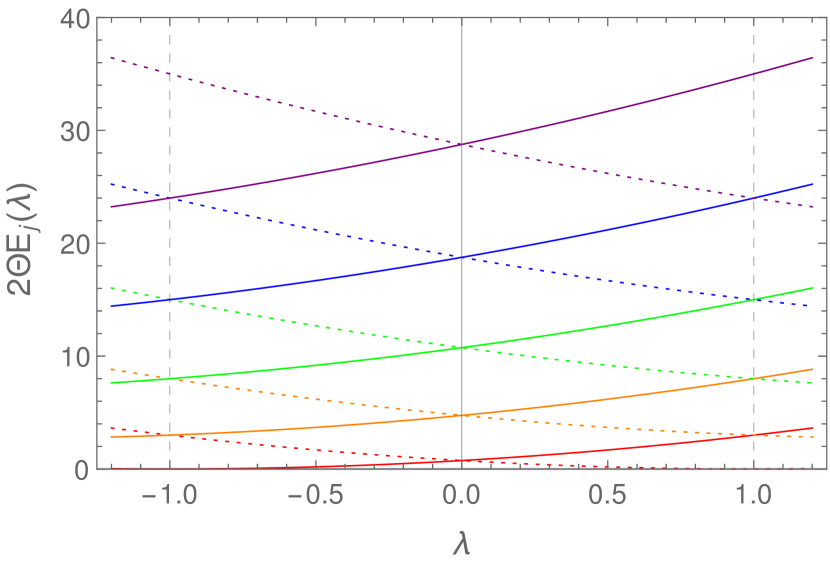
Figure 1: $\lambda$-dependence of the rotor spectrum in the presence of a nucleon (with $I=\frac{1}{2}$ and putting $E(\vec{p})=0$). The states, which are characterized by $j_{L}$ and $j_{R}=j_{L}-\frac{1}{2}$ (solid lines) or $j_{R}=j_{L}+\frac{1}{2}$ (dotted lines), are $(2j_{L}+1)(2j_{R}+1)$-fold degenerate. The solid and dotted lines that intersect at $\lambda=0$ have the same $j=j_{L}+j_{R}\in\{\frac{1}{2},\frac{3}{2},\dots\}$, with $j$ increasing by 1 as one progresses from one energy $E_{j}(0)$ to the next. Interestingly, the solid and dotted lines also intersect at $\lambda=\pm 1$, now with the corresponding $j$ values differing by 1.

5 Rotor Spectrum in the Presence of a Baryon
with Arbitrary Isospin

In this section, we consider baryons of arbitrary isospin, but still with spin $\frac{1}{2}$, which includes the $I=1$ $\Sigma$ baryon in QCD. We extend the mathematical analysis to arbitrarily large values of the isospin, even if corresponding baryons are not present in the QCD spectrum. The physical $\Sigma$ baryon is stable against strong decays, e.g. into a $\Lambda$ baryon and a pion, which is energetically forbidden. In the chiral limit of massless up and down quarks (but still with a massive strange quark), on the other hand, the pions are massless and the decay becomes possible. In a periodic volume, the decay process is affected by momentum quantization [24, 25]. For the moment, we neglect the decay channel $\Sigma\rightarrow\Lambda\pi$, and concentrate entirely on how the precession of the chiral order parameter is influenced by a baryon of arbitrary isospin $I$.

Following the construction in Section 2, for general isospin $I$ the Lagrange function takes the form

$$L=\frac{3\Theta}{8I(I+1)(2I+1)}\mbox{Tr}[\partial_{t}O^{\dagger}\partial_{t}O]+\Psi^{\dagger}\left[E(\vec{p})-i\partial_{t}-i\nu_{t}-i\lambda\vec{\sigma}\cdot\vec{e}_{p}\alpha_{t}\right]\Psi\ .$$ (5.1)

The relation

$$\mbox{Tr}[T_{a}T_{b}]=\frac{I(I+1)(2I+1)}{3}\delta_{ab}$$ (5.2)

gives rise to the prefactor of the term proportional to $\Theta$, where

$$\frac{I(I+1)(2I+1)}{3}=\sum_{I_{3}=-I}^{I}I_{3}^{2}\ .$$ (5.3)

In analogy to the $I=\frac{1}{2}$ case, it is straightforward to derive a Hamiltonian from the Lagrange function of eq.(5.1). The result is very simple: the Hamiltonian as well as the generators $\vec{L}$ and $\vec{R}$ of chiral rotations retain the same form as in the isospin $\frac{1}{2}$ case, except that $\frac{1}{2}\vec{\tau}$ is replaced by the corresponding isospin $I$ representation $\vec{T}$. For $\lambda=0$ the Hamiltonian then takes the form

$$H(0)=\frac{1}{2\Theta}\left(\vec{J}^{2}+\vec{K}^{2}-I(I+1)\right)+E(\vec{p})\ .$$ (5.4)

The resulting energy spectrum is thus given by

$$E_{j_{L},j_{R}}(0)=\frac{1}{\Theta}\left(j_{L}(j_{L}+1)+j_{R}(j_{R}+1)-\frac{1}{2}I(I+1)\right)+E(\vec{p})\ .$$ (5.5)

In the vacuum case, we had $I=0$ and $j_{L}=j_{R}$, while for the nucleon (with isospin $I=\frac{1}{2}$) we had $j_{L}=j_{R}\pm\frac{1}{2}$. For arbitrary isospin, we have $j_{L}=j_{R}+\Delta$, where $\Delta\in\{-I,-I+1,\dots,I\}$. These restrictions follow from relations between the two Casimir operators $C_{1}$ and $C_{2}$. For the vacuum case (with $I=0$) we had $C_{2}=0$, and for the nucleon (with $I=\frac{1}{2}$) we had $C_{2}^{2}-\frac{1}{2}C_{1}-\frac{3}{16}=0$. For $I=1$ the allowed values of $\Delta$ are $0$ and $\pm 1$. In this case, the constraint on $\Delta$ follows from the relation

$$C_{2}(C_{2}^{2}-2C_{1})=0\ ,$$ (5.6)

which is possible (but somewhat tedious) to verify explicitly. When $C_{2}=0$ (which was the constraint in the $I=0$ case), one obtains $\Delta=0$. When $C_{2}^{2}-2C_{1}=0$, on the other hand, one obtains $\Delta=\pm 1$. In order to satisfy eq.(5.6), one of these two constraints must be satisfied, and hence, for $I=1$, we indeed obtain $\Delta\in\{-1,0,1\}$. Similarly, for $I=\frac{3}{2}$ the two Casimir operators are related by

$$\left(C_{2}^{2}-\frac{1}{2}C_{1}-\frac{3}{16}\right)\left(C_{2}^{2}-\frac{9}{2}C_{1}+\frac{45}{16}\right)=0\ ,$$ (5.7)

which is again non-trivial to verify explicitly. We identify the first bracket as the constraint for isospin $\frac{1}{2}$ (which yields $\Delta=\pm\frac{1}{2}$), while $\Delta=\pm\frac{3}{2}$ when the second bracket vanishes. As a result, for $I=\frac{3}{2}$ eq.(5.7) indeed implies $\Delta\in\{-\frac{3}{2},-\frac{1}{2},\frac{1}{2},\frac{3}{2}\}$. In the $I=2$ case this story continues and the constraint now takes the form

$$C_{2}(C_{2}^{2}-2C_{1})(C_{2}^{2}-8C_{1}+12)=0\ .$$ (5.8)

We identify the first two factors as the constraints that give rise to $\Delta=0,\pm 1$, while $\Delta=\pm 2$ when the third factor vanishes. This implies that $\Delta\in\{-2,-1,\dots,2\}$ for $I=2$. Finally, for arbitrary integer isospin $I$, $\Delta\in\{-I,-I+1,\dots,I\}$ follows from the constraint

$$C_{2}\prod_{\Delta\in\{1,2,\dots,I\}}[C_{2}^{2}-\Delta^{2}(2C_{1}+1-\Delta^{2})]=0\ ,$$ (5.9)

while for half-integer isospin the constraint takes the form

$$\prod_{\Delta\in\{\frac{1}{2},\frac{3}{2},\dots,I\}}[C_{2}^{2}-\Delta^{2}(2C_{1}+1-\Delta^{2})]=0\ ,$$ (5.10)

Again using $j=j_{L}+j_{R}$ the corresponding energy spectrum for arbitrary isospin is given by

$$E_{j}(0)=\frac{1}{2\Theta}\left[j(j+2)+\Delta^{2}-I(I+1)\right]+E(\vec{p})\ .$$ (5.11)

For $\lambda\neq 0$ the Hamiltonian takes the form

$$H(\lambda)=H(0)+\frac{1}{2\Theta}\left(\lambda C+\lambda^{2}I(I+1)\right)\ ,$$ (5.12)

and again $C=2(\vec{\sigma}\cdot\vec{e}_{p})\vec{J}\cdot\vec{K}$. Hence, the energy spectrum now results as

$$E_{j}(\lambda)=\frac{1}{2\Theta}\left[j^{\prime}(j^{\prime}+2)+(\lambda^{2}-1)[I(I+1)-\Delta^{2}]\right]\ ,$$ (5.13)

where $j^{\prime}=j+\lambda\Delta$. The $\lambda$-dependence of the spectrum is illustrated in Fig.2 for $I=1$ and in Fig.3 for $I=\frac{3}{2}$.

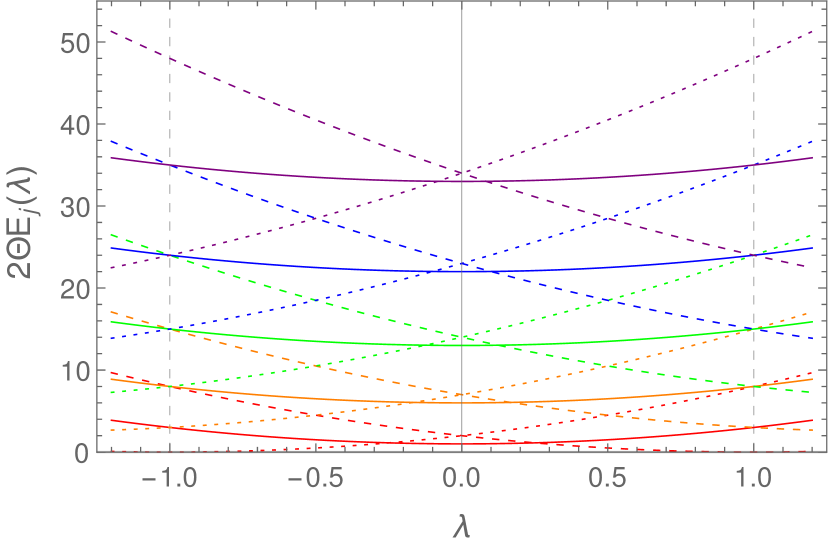
Figure 2: $\lambda$-dependence of the rotor spectrum in the presence of a $\Sigma$ baryon (with $I=1$, putting $E(\vec{p})=0$). The states, which are characterized by $j_{L}$ and $j_{R}=j_{L}$ (solid lines), $j_{R}=j_{L}-1$ (dotted lines), or $j_{R}=j_{L}+1$ (dashed lines), are $(2j_{L}+1)(2j_{R}+1)$-fold degenerate. The dashed and dotted lines that intersect at $\lambda=0$ as well as the solid line below them have the same value $j=j_{L}+j_{R}\in\{1,2,\dots\}$, with $j$ increasing by 1 as one progresses from one set of three lines to the next. As before, the lines intersect again at $\lambda=\pm 1$.

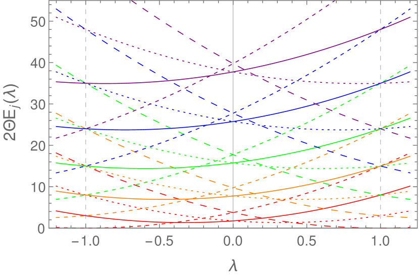
Figure 3: $\lambda$-dependence of the rotor spectrum in the presence of a baryon with $I=\frac{3}{2}$ (putting $E(\vec{p})=0$). The states, which are characterized by $j_{L}$ and $j_{R}=j_{L}-\frac{3}{2}$ (short-dashed lines), $j_{R}=j_{L}-\frac{1}{2}$ (solid lines), $j_{R}=j_{L}+\frac{1}{2}$ (dotted lines), or $j_{R}=j_{L}+\frac{3}{2}$ (long-dashed lines), are $(2j_{L}+1)(2j_{R}+1)$-fold degenerate. The solid and dotted lines that intersect at $\lambda=0$ as well as the short- and long-dashed lines that intersect above them all have the same value $j=j_{L}+j_{R}\in\{\frac{3}{2},\frac{5}{2},\dots\}$, with $j$ increasing by 1 as one progresses from one set of four lines to the next. As before, the lines intersect again at $\lambda=\pm 1$.

6 Nature of the Berry Gauge Field

Let us inspect the Berry gauge field in some detail. First of all, although it is not a dynamical field, we investigate its Yang-Mills action

$$S_{YM}[A]=-\int_{S^{3}}d\alpha d\theta d\varphi\sqrt{|g|}\frac{1}{4}\mbox{Tr}[F_{ij}F^{ij}]\ ,$$

$$\sqrt{|g|}=\sin^{2}\alpha\sin\theta\ ,$$ (6.1)

where $|g|$ is the determinant of the metric on the 3-sphere $S^{3}$ (the $SU(2)$ group manifold) with

$$g^{ij}=\mbox{diag}(g^{\alpha\alpha},g^{\theta\theta},g^{\varphi\varphi})=\mbox{diag}\left(1,\frac{1}{\sin^{2}\alpha},\frac{1}{\sin^{2}\alpha\sin^{2}\theta}\right)\ .$$ (6.2)

We read off the Yang-Mills Lagrange density

$${\cal L}_{YM}=-\frac{1}{4}\sqrt{|g|}\mbox{Tr}[F_{ij}F^{ij}]=-\frac{1}{4}\sqrt{|g|}\mbox{Tr}[F_{ij}g^{ik}g^{jl}F_{kl}]=\frac{3}{4}(1-\lambda^{2})^{2}\sin^{2}\alpha\sin\theta\ ,$$ (6.3)

which is constant over $S^{3}$, because it is proportional to the measure factor $\sin^{2}\alpha\sin\theta$. The Yang-Mills action of the Berry gauge field then takes the value $S_{YM}[A]=\frac{3\pi^{2}}{2}(1-\lambda^{2})^{2}$.

Let us also consider the Chern-Simons action

$$S_{CS}[A]=-2\lambda(\vec{\sigma}\cdot\vec{e}_{p})\int_{S^{3}}d\alpha d\theta d\varphi\sqrt{|g|}\frac{1}{8\pi^{2}}\tilde{\varepsilon}^{ijk}\mbox{Tr}\left[A_{i}\partial_{j}A_{k}+\frac{2}{3}A_{i}A_{j}A_{k}\right],$$

$$\tilde{\varepsilon}^{ijk}=\frac{\varepsilon^{ijk}}{\sqrt{|g|}}\ .$$ (6.4)

Here $\tilde{\varepsilon}^{ijk}$ is the antisymmetric tensor that transforms covariantly under general coordinate transformations, while $\varepsilon^{ijk}\in\{0,\pm 1\}$ is the ordinary antisymmetric Levi-Civita symbol. Just as in eq.(6.3), the trace in eq.(6) refers only to isospin but not to spin. Therefore, the expression for the Chern-Simons action still involves the matrix-valued prefactor $(\vec{\sigma}\cdot\vec{e}_{p})$. While this may seem strange, it is mathematically and physically fully consistent in this context. In particular, if we quantize the baryon’s spin in the direction $\vec{e}_{p}$ of its momentum vector, $(\vec{\sigma}\cdot\vec{e}_{p})$ reduces to a simple sign $\pm 1$ that characterizes the baryon’s helicity. We now read off the Chern-Simons Lagrange density

$${\cal L}_{CS} = -2\lambda(\vec{\sigma}\cdot\vec{e}_{p})\frac{1}{8\pi^{2}}\varepsilon^{ijk}\mbox{Tr}\left[A_{i}\partial_{j}A_{k}+\frac{2}{3}A_{i}A_{j}A_{k}\right]$$ (6.5)

$$= \lambda^{2}\frac{1}{8\pi^{2}}\left((1-\lambda^{2})\sin^{2}\alpha+2\sin^{2}\frac{\alpha}{2}\right)\sin\theta\ .$$

Since the Berry vector potential itself also contains the matrix-valued term $(\vec{\sigma}\cdot\vec{e}_{p})$, and since $(\vec{\sigma}\cdot\vec{e}_{p})^{2}={\mathbbm{1}}$, the actual value of the Chern-Simons term is proportional to the unit-matrix in spin space. The value of the Chern-Simons action for the Berry gauge field is given by $S_{CS}[A]=\frac{\lambda^{2}}{4}(3-\lambda^{2})$.

Remarkably, the Berry gauge field solves the Yang-Mills-Chern-Simons classical equations of motion on the curved “space-time” $S^{3}$

$$D_{j}\left(\sqrt{|g|}F^{ij}\right)=\partial_{j}\left(\sqrt{|g|}F^{ij}\right)+\sqrt{|g|}[A_{j},F^{ij}]=J^{i}\ ,$$

$$J^{i}=-2\lambda(\vec{\sigma}\cdot\vec{e}_{p})\varepsilon^{ijk}F_{jk}\ .$$ (6.6)

Here $D_{j}$ is a covariant derivative and $J^{i}$ is the current induced by the Chern-Simons term. The Chern-Simons term itself is not gauge invariant. It changes by $2\lambda(\vec{\sigma}\cdot\vec{e}_{p})$ times the integer winding number

$$n[\Omega] = \frac{1}{24\pi^{2}}\int_{S^{3}}d\alpha d\theta d\varphi\sqrt{|g|}\tilde{\varepsilon}^{ijk}\mbox{Tr}\left[(\Omega\partial_{i}\Omega^{\dagger})(\Omega\partial_{j}\Omega^{\dagger})(\Omega\partial_{k}\Omega^{\dagger})\right]$$ (6.7)

$$= \frac{1}{24\pi^{2}}\int_{S^{3}}d\alpha d\theta d\varphi\varepsilon^{ijk}\mbox{Tr}\left[(\Omega\partial_{i}\Omega^{\dagger})(\Omega\partial_{j}\Omega^{\dagger})(\Omega\partial_{k}\Omega^{\dagger})\right]$$

$$\in \Pi_{3}[S^{3}]={\mathbb{Z}}\ ,$$

of the gauge transformation function $\Omega\in SU(2)$. Although the Chern-Simons action is not invariant under large gauge transformations, the resulting classical equation of motion is gauge covariant. It is important to point out that, in this context, the prefactor of the Chern-Simons term need not be quantized, because the Berry gauge field is not a dynamical quantum field. Under a gauge transformation the various fields transform as

$$A_{i}^{\prime}=\Omega(A_{i}+\partial_{i})\Omega^{\dagger}\ ,\quad F_{ij}^{\prime}=\Omega F_{ij}\Omega^{\dagger}\ ,\quad J_{i}^{\prime}=\Omega J_{i}\Omega^{\dagger}\ .$$ (6.8)

The current $J^{i}$ is covariantly conserved, i.e.

$$D_{i}J^{i}=0\ ,$$ (6.9)

as a consequence of the non-Abelian Bianchi identity

$$\varepsilon^{ijk}D_{i}F_{jk}=0\ ,$$ (6.10)

which is automatically satisfied for any non-Abelian field strength $F_{ij}=\partial_{i}A_{j}-\partial_{j}A_{i}+[A_{i},A_{j}]$.

While the term proportional to $(\lambda^{2}-1)$ in eq.(6.5) is constant over the 3-sphere, the other term is not, because it is not just proportional to the measure factor $\sin^{2}\alpha\sin\theta$. This term, which is proportional to $\sin^{2}\frac{\alpha}{2}\sin\theta$, is even singular at $\alpha=\pi$, which corresponds to the south-pole of the 3-sphere. Since the Yang-Mills Lagrange density of eq.(6.3) is constant, this singularity is just a gauge artifact, which can be attributed to a Dirac string that passes through the south-pole of $S^{3}$. The Dirac string emanates from the origin of ${\mathbb{R}}^{4}$ in which we can embed $S^{3}$. In this sense, the Berry gauge field configuration is reminiscent of a “magnetic monopole” at the center of the 3-sphere. However, unlike the usual Dirac monopole, this object lives in 4 instead of 3 “spatial” dimensions. In any case, since the Berry gauge field is not a physical object in space-time, it does not make too much sense to discuss its physical nature as a “monopole”. Still, we find it remarkable that the Berry gauge field is the solution of a classical equation of motion on $S^{3}$. Interestingly, in another context a Berry gauge field has been identified as the BPS monopole solution of a Yang-Mills theory coupled to an adjoint Higgs field [9]. In that case, besides the Berry gauge field, the states of the quantum mechanical system also give rise to an adjoint Higgs field as a “Berry matter field” which provides a covariantly conserved current in the Yang-Mills-Higgs equation of motion. In our case, instead of “Berry matter” the Chern-Simons term of the Berry gauge field provides a conserved current. While it would be interesting to further investigate the Berry gauge field of eq.(4) in a dynamical context, for our present purposes the above characterization of its geometrical and topological features is sufficient.

7 Conclusions

We have investigated the rotor spectrum of QCD with two massless and one massive flavor in a periodic volume in the baryon number 1 sector, for different values of the isospin $I=\frac{1}{2},1,\frac{3}{2},2,\dots$, thus generalizing the $I=\frac{1}{2}$ results of [2]. The presence of a baryon manifests itself by a Berry gauge field in the effective rotor Hamiltonian. Interestingly, the Berry gauge field solves an abstract Yang-Mills-Chern-Simons equation of motion in the group space $S^{3}$ of $SU(2)$.

It would be interesting to further investigate the QCD spectrum in the chiral limit. In particular, the single-pion states also belong to a tower of rotor states, presumably again with a non-trivial Berry gauge field. In addition, it would be interesting to incorporate transitions between baryons of different isospin, such as $\Sigma\rightarrow\Lambda\pi$, induced by pion emission and absorption, and study the corresponding effects on the Berry gauge field. Furthermore, one can consider QCD with three massless flavors and investigate the precession of the chiral order parameter in the corresponding $SU(3)$ vacuum manifold. In all these cases, one can ask whether the resulting Berry gauge fields again solve a classical equation of motion.

In principle, our analytic results can have an impact on the analysis of lattice QCD data, which, however, are difficult to obtain in the chiral limit. In order to make contact with lattice QCD, it would therefore be interesting to extend the analytic calculations by including explicit chiral symmetry breaking effects due to non-zero up and down quark masses. While our results in the strict chiral limit are mostly of academic interest, they shed new light on the concept of Berry gauge fields and its manifestation in non-trivial quantum field theories including QCD.

References

[1]
H. Leutwyler, Phys. Lett. B189 (1987) 197.
[2]
S. Chandrasekharan, F.-J. Jiang, M. Pepe, and U.-J. Wiese, Phys. Rev. D78
(2008) 077901.
[3]
M. Berry, Proc. Roy. Soc. London, Ser. A392 (1984) 45.
[4]
B. Simon, Phys. Rev. Lett. 51 (1983) 2167.
[5]
P. Hasenfratz and F. Niedermayer, Z. Phys. B92 (1993) 91.
[6]
G. Herzberg and H. C. Longuet-Higgins, Discuss. Faraday Soc. 35 (1963) 77.
[7]
C. Mead, Chem. Phys. 49 (1980) 23; 33.
[8]
J. Moody, A. Shapere, and F. Wilczek, Phys. Rev. Lett. 56 (1986) 893.
[9]
J. Sonner and D. Tong, Phys. Rev. Lett. 102 (2009) 191801.
[10]
J. Gasser and H. Leutwyler, Nucl. Phys. B250 (1985) 465.
[11]
J. Gasser, M. E. Sainio, and A. Svarc, Nucl. Phys. B307 (1988) 779.
[12]
E. Jenkins and A. Manohar, Phys. Lett. B255 (1991) 558.
[13]
E. Jenkins, Nucl. Phys. B368 (1992) 190.
[14]
V. Bernard, N. Kaiser, J. Kambor, and U.-G. Meissner, Nucl. Phys. B388
(1992) 315.
[15]
S. Chandrasekharan, M. Pepe, F. Steffen, and U.-J. Wiese, JHEP 0312 (2003)
035.
[16]
P. Hasenfratz, Nucl. Phys. B828 (2010) 201.
[17]
F. Niedermayer and C. Weiermann, Nucl. Phys. B842 (2011) 248.
[18]
F. Niedermayer and P. Weisz, arXiv:1801.06858 [hep-th].
[19]
M. Weingart, PoS LATTICE2010 (2010) 094; arXiv:1006.5076 [hep-lat].
[20]
M. E. Matzelle and B. C. Tiburzi, Phys. Rev. D93 (2016) 034506.
[21]
A. Hasenfratz, P. Hasenfratz, F. Niedermayer, D. Hierl, and
A. Schäfer, PoS LATTICE2006 (2006) 178.
[22]
W. Bietenholz, M. Göckeler, R. Horsley, Y. Nakamura, D. Pleiter,
P. E. L. Rakow, G. Schierholz, and J. M. Zanotti,
Phys. Lett. B687 (2010) 410.
[23]
W. Bietenholz, N. Cundy, M. Göckeler, R. Horsley, Y. Nakamura,
D. Pleiter, P. E. L. Rakow, G. Schierholz, and J. M. Zanotti,
J. Phys. Conf. Ser. 287 (2011) 012016.