Abstract

Applying the Born-Infeld Anti de Sitter charged black hole metric we calculate holographic entanglement entropy (HEE) by regarding the proposal of Ryu and Takanayagi. To do so we assume that time dependence of the black hole mass and charge to be as step function. Our work is restricted to small subregions where a collapsing null shell dose not penetrate the black holes horizon. To calculate time dependent HEE we use perturbation method for small subregions where turning point is much smaller than local equilibrium point of black hole. We choose two shape functions for entangled regions on the boundary which are the strip and the ball regions. There is a saturation time at which the null shell grazes the turning point and the HEE reaches to its maximum value. In general, this work satisfies result of the works presented by Camelio et al and Zeng et al. We must point out that they used equal time two-point correlation functions and Wilson loops instead of the entanglement entropy (EE) as non-local observable to study this thermalization by applying the numerical method.

1 Introduction

Duality correspondence between an Anti de Sitter spacetime in bulk and boundary conformal field theory (AdS/CFT) is a conjecture where a gravity theory defined on the AdS bulk space time corresponds to a quantum field theory defined on its asymptotic boundary region [1,2]. In fact the AdS/CFT duality relates quantum physics of strongly coupled many-body systems to the classical dynamics of a gravitational model which lives in one higher dimension. It is a suitable way to understand and to study quantum gravity [3], because one can argue unknown quantum gravity which is described entirely by a topological quantum field theory, in which all physical degrees of freedom are projected onto the boundary. The entanglement entropy (EE) or von Neumann entropy of quantum microstates of boundary CFT behaves as a non-local observable same as the equal time Wightman two-point correlation functions [4,5] and Wilson loops [6]. The EE is a very important quantity to understand the physical nature of thermalization of a non-equilibrium quantum system [7-17], superconducting phase transition [18-26] and cosmological singularity [27,28]. Geometrizing EE can be possible by applying the holographic approach. In this prescription the EE obtained from the field theory under consideration corresponds to a minimal surface defined in the bulk geometry which is anchored to the entangled region. The holographic approach presented by Ryu and Takayanagi leads to similarity between the Bekenstein-Hawking entropy of static AdS black holes and the EE of microstates of the dual boundary time-independent quantum conformal fields [29] (see also [30]). To calculate time dependent EE the Takayanagi et al proposal is given in ref. [31] for time dependent AdS/CFT correspondence where minimal surface evaluates versus the time until equilibrates. With the above conditions, the minimal surface can penetrate into the event horizon and gives information from the black hole structure to the observer far from the horizon without exhibits the black hole singularity. Evolving the EE and the dynamical process in the bulk is described by a global quantum quench on the boundary. Actually the initial static background in the pure AdS state is perturbed by a time-dependent disturbance which is produced by injecting uniform energy density at the initial time. These global quenches on the boundary are modeled by a collapsing null shell of matter which initially are located on the boundary and causes to form a black hole at the center of the AdS space time [32,33,34]. If the energy density injection occurs instantaneously, then the corresponding disturbance will be sharp which is in accord to collapse of a very thin shell, while smooth perturbations read to specified thickness shell.
Entanglement evolution obtained from global quantum quench is studied in [35] for a transverse Ising spin chain in 1+1-dimensional CFT in which the EE grows linearly versus the time $\Delta S(t)\approx t$ and is proportional to final thermal entropy density at saturation time $t_{sat}$. The saturation time is particular time where the system reaches to an equilibrium state and so EE does not evolve more. Its maximum value is proportional to the size of entangled region. In general, rate of EE growth means speed of time evolution of the EE which is defined by $\Re(t)\sim\frac{d}{dt}\Delta S(t).$ In fact $\Re(t)$ maybe take on numerical values $\Re(t)\leq 1$ which satisfies causality constraint condition of the holographic system [36,37] while there maybe are situations for which the causality constraint condition breaks and maximum value of the HEE velocity raises to some values bigger that the light velocity. In tsunami picture in which the evolution of EE is pictured as an inward moving from the boundary with ‘tsunami‘ velocities $\Re(t)\leq 1$ and we can see for the large subsystems in [14, 51]. The situation is different in small subsystems which we will consider here. First we define $t_{theq}$ as characteristic time of thermal equilibrium state of the small subsystem. Now due to the size of the entangled region is much smaller than the thermal excitations $t_{sat}\ll t_{theq},$ therefore the interactions counterpart become negligible and so the system takes on its saturate state before the thermal excitations can affect.
Camilo et al studied holographic thermalization of the Born-Infeld AdS black hole in the presence of a chemical potential (the electric charge effect) [38]. They used equal time two-point correlation functions and expectation values of Wilson loop operators as the non-local observable to probe the black hole thermalization. They used numerical method to calculate the dynamical equations and the HEE of the system. They showed that as the charge and the Born Infeld parameter grow, the thermalization time bears an increase and decrease, respectively. They obtained similar result by applying the HEE as the other non-local observable instead of the Wilson loop and two point correlation function. They exhibited existence of a phase transition point which is depended to numerical values of the charge $Q$ and the Born-Infeld parameter $b$. This point divides the thermalization process into an accelerating and a decelerating phase. As non-local observable the two point correlation function and the HEE are used also to study phase transition of the AdS Born-Infeld black hole by Zeng et al [39]. They obtained that it is happened for $bQ>0.5$ but not for $bQ<0.5.$ In the latter case there is a new branch for the infinitesimally small black hole so that a pseudo phase transition emerges besides the original Hawking-Page phase transition. At last they can infer that the phase structure of the non-local observable is similar to that of the thermal entropy regardless of the size of the boundary region in the field theory.
Here we explore the bulk geometry by applying the Non-linear Maxwell-Einstein (Born-Infeld) gravity theory [40,41]. Then we calculate HEE of a Born-Infeld charged AdS black hole made from null shell collapsing matter. This null shell matter is assumed to be originated from injection of a matter field on the CFT side of the AdS space as suddenly. It must be noticed that the time dependence null shell profiles which we consider here, vanishes any non-monotonic behaviors during the quench [61], and could get our calculation as simple and lead to a neat result containing all of issues which we seek them. To do so the time dependence for the mass and the charge of the black hole is assumed to have a step function form. This means that the matter source is injected suddenly at the initial time into the vacuum AdS space time to make a black hole. To calculate the HEE we should choose a shape function for a subregion on the holographic side. In usual way we choose the strip and the ball shape for the subregions. We calculate the HEE and its evolution rate $\Re(t)$ for different values of the dimensionless Born-Infeld coupling constant $b$.
Layout of the paper is as follows. In section 2 we introduce AdS Einstein-Born-Infeld gravity theory, and corresponding spherically symmetric static black hole metric solution [40,41,42]. We use infinite volume limit proposed by Witten [43] to calculate the effective counterpart of the spherically symmetric static Born-Infeld black hole metric. It is useful to obtain its asymptotically AdS form. Then we calculate the corresponding Hawking temperature. We will use Eddington-Finkelstein coordinates system to obtain the perturbed metric of the bulk AdS space time via a collapsing null shell in the presence of nonlinear electromagnetic field. At last we calculate the location of turning point $z_{t}$ with respect to the black hole horizon $z_{h}$, mass of the collapsing thin shell $M$, the Born-Infeld coupling constant $b$ and the AdS radius $L$. For small subregions we have $z_{t}\ll z_{h}$ which makes us capable to use perturbation method to calculate the HEE. In section 3 we use Takayanagi et al proposal to obtain a perturbation series solution for the time dependent HEE of the Born-Infeld AdS black hole. Section 4 denotes to conclusion of the work and some outlooks which we consider for the future work.

2 AdS-Einstein-Born-Infeld gravity

Let us we start with a non-linear Maxwell action minimally coupled with the Einstein-Hilbert gravity action in the presence of a cosmological constant described in a 4D curved space time as follows [40,41].

$$S=\int d^{4}x\sqrt{-g}\bigg{[}\frac{R_{\mu}^{\mu}-2\Lambda}{16\pi G}+4b^{2}\bigg{(}1-\sqrt{1+\frac{2F}{b^{2}}}\bigg{)}\bigg{]},$$ (2.1)

where $R_{\mu}^{\mu}$ is Ricci scalar, $F=\frac{1}{4}F_{\mu\nu}F^{\mu\nu}$ is the Maxwell electromagnetic field lagrangian density and $b$ is the Born-Infeld parameter. $G$ is Newton‘s coupling constant and $\Lambda$ is the cosmological constant which relates to radius of the 4D-AdS space time $L$ as $\Lambda=-\frac{3}{L^{2}}$ [41]. One can infer for $b\to\infty$ the last term of the above action leads to $4b^{2}[1-\sqrt{1+2F/b^{2}}]\sim-4F+O(b^{-2})$ and so the total action reduces to the well known Einstein-Maxwell model. Author of the ref. [41] obtained a spherically symmetric static charged black hole metric of the model (2.1) as follows.

$$ds^{2}=-f(r)dt^{2}+\frac{dr^{2}}{f(r)}+r^{2}d\Omega_{2}^{2},$$ (2.2)

where $d\Omega_{2}^{2}=(d\theta^{2}+\sin^{2}\theta d\phi^{2})$ denotes to the unit 2-sphere metric $\mathbb{S}^{2}$, and $f(r)=1+g(r)$ for which

$$g(r)=-\frac{2M}{r}+\frac{r^{2}}{L^{2}}+\frac{2b^{2}r^{2}}{3}\bigg{(}1-\sqrt{\frac{Q^{2}}{b^{2}r^{4}}+1}\bigg{)}+\frac{4Q^{2}}{3r^{2}}~{}{}_{2}F_{1}\bigg{(}\frac{1}{4},\frac{1}{2},\frac{5}{4};-\frac{Q^{2}}{b^{2}r^{4}}\bigg{)}.$$ (2.3)

${}_{2}F_{1}(r)$ given in the above metric potential is hypergeometric function, $M$ and $Q$ are constants of integral. They have related to the black hole mass and the electric charge respectively. It is simple to calculate asymptotically behavior of the metric potential $f(r)$ at infinity $r\to\infty$ as $f(r)\sim 1-\frac{2M}{r}+\frac{Q^{2}}{r^{2}}+\frac{r^{2}}{L^{2}}-\frac{Q^{4}}{20b^{2}r^{6}}$ which leads to a Reissner-Nordström AdS black hole in limits $b\to\infty$ [41]. One can obtain nonzero component of the electromagnetic field of the system as $F^{rt}=\frac{b}{\sqrt{1+b^{2}r^{4}/Q^{2}}}.$ It is equivalent with the vector potential gauge field $A_{\mu}(r)=(A_{t}(r),0,0,0)$ as $F^{rt}(r)=-\frac{dA_{t}(r)}{dr}.$ We can integrate it to obtain $A_{t}(r)=\frac{Q}{r}{}_{2}F_{1}(\frac{1}{4},\frac{1}{2},\frac{4}{4};-\frac{Q^{2}}{b^{2}r^{4}})-\Phi$ in which $\Phi$ is a constant of integral. It is really electrostatic potential difference between the horizon and infinity of the charged Born-Infeld black hole. $A_{t}(r)$ is a gauge field and so we can set $A_{t}(r_{h})=0$ on the black hole horizon $r_{h}$ obtained from $f(r_{h})=0$ (see [38,41] for more details.) By applying the latter boundary condition one can infer

$$\Phi(r_{h})=\frac{Q}{r_{h}}~{}{}_{2}F_{1}\bigg{(}\frac{1}{4},\frac{1}{2},\frac{5}{4};-\frac{Q^{2}}{b^{2}r_{h}^{4}}\bigg{)}.$$ (2.4)

In the context of the AdS/CFT correspondence there may be exist some black holes with varied topologies for instance planer solutions [43] where their topology at the boundary of a 4D-AdS space-time are $\mathbb{R}^{3}$ instead of $\mathbb{R}\times\mathbb{S}^{2}$. Such a black hole exist only due to the presence of a negative cosmological constant. To obtain such a black hole we should usually use finite-volume re-scaling of the solutions as done in [42] by introducing a dimensionless parameter $\lambda$ and then obtain its limits at $\lambda\to\infty$. The latter proposal is well known as ”infinite volume limit” which we will consider it to obtain topologically deformed form of the metric solution (2.3). It should be reminded the Born-Infeld parameter $b$ and the AdS radius $L$ is topological invariant quantities for the metric solution (2.3) but its other quantities are changed under the transformations $\lambda$ as follows: $r\rightarrow\lambda^{1/3}r$, $t\rightarrow-\lambda^{-1/3}t$, $M\rightarrow\lambda M$, $Q\rightarrow\lambda^{2/3}Q,$ $L^{2}d\Omega_{2}^{2}\rightarrow\lambda^{-2/3}(d\vec{x}\cdot d\vec{x})$ for which $f(r)\to\lambda^{\frac{2}{3}}\big{(}\lambda^{-\frac{2}{3}}+g(r)\big{)}.$ After substituting the latter transformations into the metric solution (2.2) and taking its limits for $\lambda\to\infty$ we obtain

$$ds^{2}=-g(r)dt^{2}+\frac{dr^{2}}{g(r)}+\frac{r^{2}}{L^{2}}d\vec{x}\cdot d\vec{x},$$ (2.5)

where $g(r)$ is given by (2.3) and now the horizon defined by $g(r_{h})=0$ is planner instead of the spherical and so it should be called as black brane instead of black hole in higher dimensional gravity models. The Hawking temperature for such a black hole in the context of AdS/CFT perspective is viewed as the equilibrium temperature of the dual field theory on the boundary of 4D-AdS space-time. It is defined by $T=\frac{1}{4\pi}\frac{dg(r)}{dr}\big{|}_{r_{h}}$ which for the metric equation (2.5) reads [38],

$$T=\frac{r_{h}}{4\pi}\bigg{[}2b^{2}\bigg{(}1-\sqrt{1+\frac{Q^{2}}{b^{2}r_{h}^{4}}}\bigg{)}+\frac{3}{L^{2}}\bigg{]}.$$ (2.6)

In case where the above temperature vanishes $T=0$ then the charged Born-Infeld black hole is called as extremal black hole. It is happened at a particular charge value which its absolute value is given by

$$Q_{max}=\frac{\sqrt{3}r_{h}^{2}}{L}\sqrt{1+\frac{3}{4L^{2}b^{2}}}.$$ (2.7)

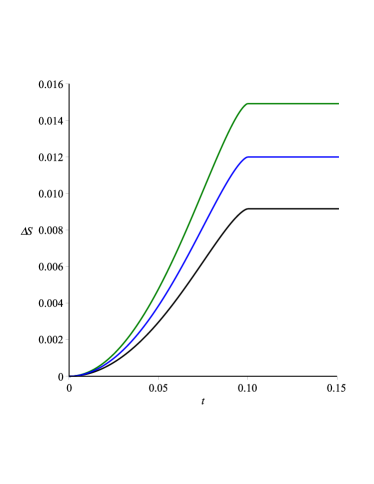
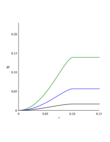
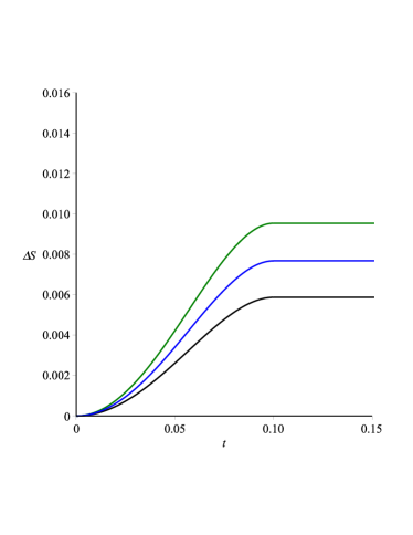
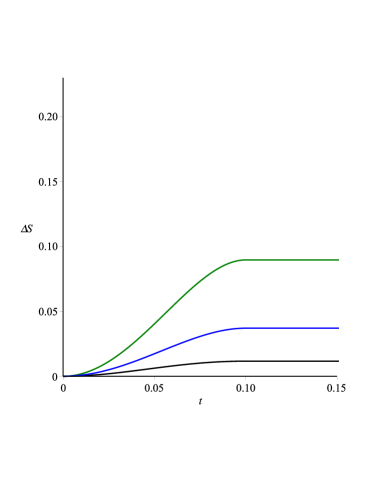
Figure 1: Growth of EE is plotted vs the time for the strip and the ball regions. In these diagrams we put $z_{t}/z_{h}=0.1$ due to small subregions and set $A_{\Sigma}/16G_{N}^{(4)}=1$. In $(a)$ and $(b)$ diagrams are plotted for the strip region and in $(c)$ and $(d)$ are plotted for disk. In $(a)$ and $(c)$ we set $Q=1$ but in $(b)$ and $(d)$ we set $Q=5$. Black, blue and green colored lines indicate $b=0.01,0.1$ and $1$ respectively.

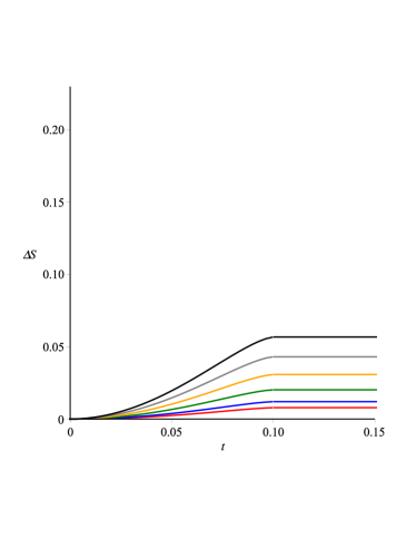
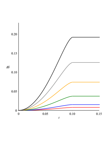
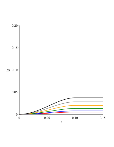
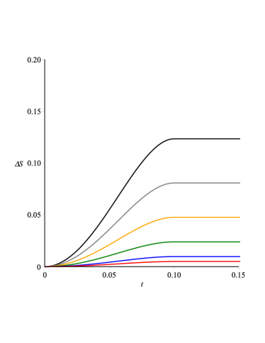
Figure 2: The evolution of EE for fixed $b=0.1$ and in the limit of $b\rightarrow\infty$ for the strip region indicated in $(a)$ and $(b)$, and for the ball region indicated in $(c)$ and $(d)$, respectively. Colored lines represent different charges as $Q=0,1,2,3,4,5$ which are indicated by red, blue, green, orange, gray and black colored lines respectively.

In general the above temperature takes on some positive values $T\geq 0$ for which we just have $0<|Q|\leq Q_{max}.$ $Q=0$ corresponds to vanishing vector potential gauge field and $|Q|=Q_{max}$ corresponds to zero temperature state respectively. In the latter case the black hole system exhibits with the thermalization when the HEE difference raises versus the time because of the thermodynamic equation $\Delta S=\frac{dE}{T}>0.$ In fact for $T>0$ the black hole absorbs the energy from the environment $\Delta E>0$ and so its HEE difference raises $\Delta S>0$ and vice versa (see figures 1 and 2). To study behavior of the metric solution (2.5) near the AdS boundary, it is convenient to introduce a new ‘inverse‘ radial coordinate like $z=L^{2}/r$ in which the singularity $r=0$ sits at infinity while AdS boundary stays at $z=0$. Applying the latter transformation the metric solution (2.5) reads

$$ds^{2}=\frac{L^{2}}{z^{2}}\bigg{[}-F(z)dt^{2}+\frac{dz^{2}}{F(z)}+d\vec{x}\cdot d\vec{x}\bigg{]},$$ (2.8)

where,

$$F(z)=\frac{z^{2}}{L^{2}}g(L^{2}/z)=1-\frac{2Mz^{3}}{{L^{4}}}+\frac{4Q^{2}z^{4}}{3L^{6}}~{}{}_{2}F_{1}\bigg{(}\frac{1}{4},\frac{1}{2},\frac{5}{4};-\frac{Q^{2}z^{4}}{b^{2}L^{8}}\bigg{)}$$

$$+\frac{2b^{2}L^{2}}{3}\bigg{(}1-\sqrt{\frac{Q^{2}z^{4}}{b^{2}L^{8}}+1}\bigg{)}$$ (2.9)

for which $F(z)\to 1$ near the AdS boundary $z=0.$ This means that near the AdS boundary the metric (2.8) leads to a conformaly flat form with conformal factor $\frac{L^{2}}{z^{2}}.$ In order to avoid the coordinate singularity at $r=r_{h}$ we should use the Eddington-Finkelstein coordinate system $(v,z,x_{i};i=3,4)$ with $d\upsilon=dt-dz/F(z)$ to re-write the metric solution (2.8) as follows.

$$ds^{2}=\frac{L^{2}}{z^{2}}\bigg{[}-F(z)d\upsilon^{2}-2d\upsilon dz+d\vec{x}\cdot d\vec{x}\bigg{]}.$$ (2.10)

Up to the term of conformal factor $L^{2}/z^{2},$ the above metric is usually called as Vaidya space time for time dependent metric $F(z,v)$. It describes space time metric from point of view of an accelerating observer moving toward the black hole center. In general the Hawking temperature of black holes destruct its background metric which is well known as backreaction problem (see introduction section in ref. [45]). In the particle physics perspective one can infer some interacting quantum matter fields fluctuations create particles-antiparticles near the horizon. Stress tensor of these created particles causes to shrink the horizon and so the horizon maybe eliminated finally and so one can exhibit with an essential question as follows. What is final state of an evaporating black hole? In usual way it is still an open problem and the backreaction equation $G_{\mu\nu}=<\widehat{T}^{quantum~{}field}_{\mu\nu}>_{renormalized}$ is solved analytically just for 2D black holes (see [45,46] and references therein). As a future work we encourage to study HEE of this black hole by regarding the mentioned above backreaction problem. With this correspondence the Bekenstein-Hawking entropy of an evaporating AdS black hole become equivalent with the EE of quantum microstates from CFT side. It is done when the minimal surface wrap the horizon [29]. In fact holography provides a geometric intuition for which local operators such as expectation values of the energy momentum tensor of the quantum matter fields $<\widehat{T}^{quantum~{}field}_{\mu\nu}>_{renormalized}$ are not sensitive to the thermalization process. They are only sensitive to phenomena happening near the AdS boundary. To probe the global process of thermalization one needs to consider extended non-local observables such as two point correlation functions and expectation values of rectangular Wilson loops and EE of boundary regions which have well known holographic descriptions in the dual AdS bulk perspective (see [38,42] for more discussions ). In general one use usually a collapsing thin shell to study dynamics of an evaporating quantum black hole. If the interacting quantum matter fields become charge-less then the electric charge of the quantum black hole will be invariant while its mass evaporates and so we have to put $M\to M(v)$ in the metric equation (2.11). If the quantum matter fields have electric charge (for instance complex quantum scalar fields) the quantum black hole electric charge varies for which we should replace $Q\to Q(v)$ together with the $M\to M(v)$. Authors of the paper [42] are used samples $M(\upsilon)=M(1+\tanh\frac{\upsilon}{\upsilon_{0}})/2$ and $Q(\upsilon)=Q(1+\tanh\frac{\upsilon}{\upsilon_{0}})/2$, to study holographic thermalization of a charged-Born-Infeld quantum black brane (2.11). It is clear that for $\upsilon\to-\infty$ we have pure AdS with $M(-\infty)=0=Q(-\infty)$ while for $\upsilon\to+\infty$ we have $M(+\infty)=M,Q(+\infty)=Q$. $\upsilon_{0}$ is a constant and shows the finite thickness of the shell. The Smooth form for the above mentioned sample $M(\upsilon),Q(\upsilon)$ shows that they are applicable for the numerical analysis. For a shock wave which is made from zero thickness shell of charged matter suddenly forming at $\upsilon=0$ we can usually use a step function $Q(\upsilon)=Q\theta(\upsilon)$ and $M(\upsilon)=M\theta(\upsilon)$ (see section 3.3.1 in ref. [47]) which is applicable for analytical calculations. They are asymptotic behavior of the functions $M(\upsilon)=M(1+\tanh\frac{\upsilon}{\upsilon_{0}})/2$ and $Q(\upsilon)=Q(1+\tanh\frac{\upsilon}{\upsilon_{0}})/2$, at $\upsilon_{0}\to 0$ which we will consider in this paper (see [38] for more discussions). To obtain time dependent form of the metric solution (2.11) it is convenient to evaluate mass and charge of the black hole versus the corresponding Hawking temperature (2.6) as follows.
Applying the inverse transformation $z=\frac{L^{2}}{r}$ for the event horizon $r_{h}$ obtained from $g(r_{h})=0$ one can determine location of the event horizon in the Eddington-Finkelstein coordinate system as $z_{h}=\frac{L^{2}}{r_{h}}.$ In fact $z_{h}$ is determined versus the AdS Born Infeld black hole parameters $M,Q,b,L$ by solving $F(z)=0$ given by (2.9) as follows.

$$1-\frac{2Mz_{h}^{3}}{{L^{4}}}+\frac{4Q^{2}z_{h}^{4}}{3L^{6}}~{}{}_{2}F_{1}\bigg{(}\frac{1}{4},\frac{1}{2},\frac{5}{4};-\frac{Q^{2}z_{h}^{4}}{b^{2}L^{8}}\bigg{)}+\frac{2b^{2}L^{2}}{3}\bigg{(}1-\sqrt{\frac{Q^{2}z_{h}^{4}}{b^{2}L^{8}}+1}\bigg{)}=0.$$ (2.11)

Substituting $r_{h}=\frac{L^{2}}{z_{h}}$ into the relation (2.6) we can infer:

$$T(M,Q,b,L)=\frac{3+2b^{2}L^{2}(1-\sqrt{1+Q^{2}z_{h}^{4}/b^{2}L^{8}})}{4\pi z_{h}}.$$ (2.12)

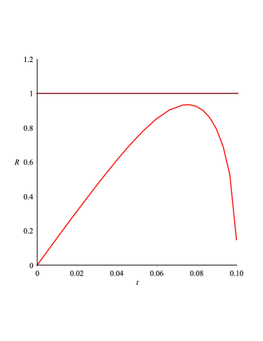
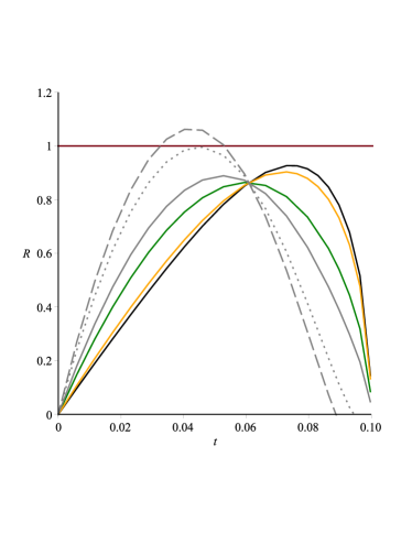
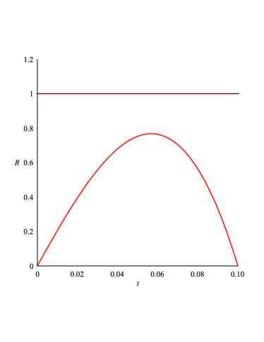
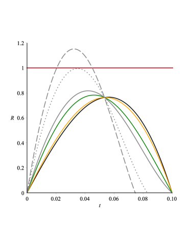
Figure 3: The rate of EE growth for $z_{t}=z_{h}=1$, horizontal lines represent the speed of light.(a) and (b) correspond to the strip region while (c) and (d) correspond to the disk region. In figures $(a)$ and $(c)$ we put $Q=1$ and plot $\Re(t)$ vs the time for all values of $b$ with red colored line. But in figures $(b)$ and $(d)$ we put $Q=5$ and $b=1,0.1,0.01$ and $0.005$ and plot $\Re(t)$ vs the time with black, orange, green and gray colored lines respectively. In $(b)$ gray-dot line corresponds to $b=0.0025$ and gray-dash line is obtained with $b=0.002$, whereas in $(d)$ $b=0.00155$ corresponds to the dot-gray and $b=0.001$ is used to plot dash-gray line.

In the collapsing thin shell model, we assume $\mathcal{R}(t)>l_{eq}$ to be the size of an evolving spacelike surface $(\Sigma,t)$ at a time ‘$t$, where $l_{eq}$ is its size at in equilibrium state. The corresponding bulk extremal surface $\gamma_{\Sigma}(t)$ can be parameterized as $(z_{t}(t),\upsilon_{t}(t))$ versus the time parameter ‘t‘. There are usually exist multiple extremal surfaces for a given $(\Sigma,t)$ for which we should choose the one with smallest area. In general there is not a simple relation between $(\mathcal{R},t)$ and $(z_{t},\upsilon_{t})$ for which we must be solve the full equations of motion for entangled area $\gamma_{\Sigma}(t).$ In a penrose diagram of the collapsing system $\gamma_{\Sigma}(t)$ trace out a curve $(z_{t}(t),\upsilon_{t}(t))$ for a given $(\Sigma,t)$ by varying the time parameter ‘t‘(See figs. 2 and 3 in ref. [14]). These figures show that the location of event horizon $(z_{h},\upsilon_{h})$ is a local equilibrium scale and so for $z_{t}=\frac{L^{2}}{R(r)},z_{h}=\frac{L^{2}}{r_{h}}$ one can infer $\frac{z_{t}}{z_{h}}<1.$ Now we are in a position to obtain time dependent form of the metric (2.11) for a collapsing thin shell with mass $M(\upsilon)$ and the charge $Q(\upsilon)$ as follows. We will try to obtain this time behavior by a perturbation method presented in [47] in which the on shell action is expanded with respect to a dimensionless perturbation parameter. In our case this parameter would be $\epsilon\equiv\frac{z_{t}}{z_{h}}\ll 1$ as it mentioned in above. By expanding the Lagrangian density and embedding functions around the vacuum case one can obtain the on-shell action as follows.

$$S_{on-shell}[\varphi(z)]=\int_{on-shell}dz\mathcal{L}[\varphi(z),\epsilon]$$

$$=\int dz\mathcal{L}^{(0)}[\varphi^{(0)}(z)]+\epsilon\int dz\mathcal{L}^{(1)}[\varphi^{(0)}(z)]+\mathcal{O}(\epsilon^{2}),$$ (2.13)

in which $\mathcal{L}$ is the Lagrangian density and $\varphi(z)$ stands for embedding functions which could be obtained by solving the Euler Lagrange equations. Neglecting higher order terms of the action functional (2.13) we can infer that leading order term of the embedding functions, $\varphi^{(0)}(z)$ is just enough to obtain on-shell action. It is enough to compatible with observation. To have a perturbation solution for the model it is better to re-write the functional with respect to the orders of $z_{t}/z_{h}$ and expand $F(z)$ defined by (2.9) as well as embedding functions order by order.
But before doing that it is convenient to evaluate mass and charge of black hole with respect to the Hawking temperature. Since Hawking temperature contains event horizon, so $z_{h}$ appears into the terms and perturbation parameter can be extracted easily. Putting $L=1$ for convenient and using (2.12) for the temperature and $F(z_{h})=0$ for the event horizon we get

$$M=\frac{\mu}{z_{h}^{3}},~{}~{}~{}\text{and}~{}~{}~{}Q^{2}=\frac{\eta}{4b^{2}z_{h}^{4}},$$ (2.14)

with

$$\eta=4\pi Tz_{h}(4\pi Tz_{h}-4b^{2}-6)+12b^{2}+9,$$

$$\mu=\frac{1}{2}+\frac{\eta}{6b^{2}}~{}{}_{2}F_{1}\bigg{(}\frac{1}{4},\frac{1}{2},\frac{5}{4};-\frac{\eta}{4b^{4}}\bigg{)}+\frac{b^{2}}{3}\bigg{(}1-\frac{1}{2}\sqrt{4+\frac{\eta}{b^{4}}}~{}\bigg{)}.$$ (2.15)

Thus by these new parameters which are functions with respect to the event horizon and the Hawking temperature, $F(\upsilon,z)$ can be rewritten as

$$F(\upsilon,z)=1-2\mu(\upsilon)\bigg{(}\frac{z}{z_{h}}\bigg{)}^{3}+\frac{\eta(\upsilon)}{3b^{2}}~{}{}_{2}F_{1}\bigg{(}\frac{1}{4},\frac{1}{2},\frac{5}{4};-\frac{\eta(\upsilon)}{4b^{4}}\bigg{(}\frac{z}{z_{h}}\bigg{)}^{4}\bigg{)}\bigg{(}\frac{z}{z_{h}}\bigg{)}^{4}$$

$$+\frac{2b^{2}}{3}\bigg{(}1-\sqrt{1+\frac{\eta(\upsilon)}{4b^{4}}\bigg{(}\frac{z}{z_{h}}\bigg{)}^{4}}~{}\bigg{)}.$$ (2.16)

Time dependence of $\eta(\upsilon)$ and $\mu(\upsilon)$ comes from time evolution of the mass and charge of black hole. We can choose this dependence in the form of step functions for simplicity as $\mu(\upsilon)=\mu~{}\theta(\upsilon)$ and $\eta(\upsilon)=\eta~{}\theta(\upsilon)$, and at last we obtain $F(z)$ again but with respect to $\eta$ and $\mu$ instead of the mass and charge.
Now by attention to what is mentioned before if $z_{t}\ll z_{h}$ and since always $z\leqslant z_{t}$ therefore $(z/z_{h})\ll 1$, and by keeping two first term from expansion of (2.16) we get to

$$F(\upsilon,z)=1-2\mu~{}\theta(\upsilon)\bigg{(}\frac{z}{z_{h}}\bigg{)}^{3}+\frac{\eta~{}\theta(\upsilon)}{4b^{2}}\bigg{(}\frac{z}{z_{h}}\bigg{)}^{4}+\mathcal{O}\bigg{(}\frac{z}{z_{h}}\bigg{)}^{8}.$$ (2.17)

Zero order term in the above equation as expected represents pure AdS solution which is static and will not change over time. We can take $\epsilon\equiv(z_{t}/z_{h})^{3}$ as dimensionless perturbation parameter. The next term is in order of $(z_{t}/z_{h})^{4}=\epsilon^{\frac{4}{3}}$ which is located before the term $\epsilon^{2}$. In fact it is still first order and without loss of generality it can be rewritten as $(z^{4}/z_{h}z_{t}^{3})\epsilon$. Therefore we must treat with this term as the first order and use exactly the same embedding functions of pure AdS in the first order approximation.

3 Time dependent HEE

According to the Ryu and Takayanagi proposal [29] in the context of AdS/CFT correspondence, the EE of a region on the boundary is defined by

$$S_{EE}=\frac{1}{4G_{N}^{(d)}}\int_{\Sigma}d\zeta^{d-2}\sqrt{h}=\frac{1}{4G_{N}^{(4)}}\int_{\Sigma}dz\bigg{(}\mathcal{L}^{(0)}+\epsilon\theta(\upsilon)\mathcal{L}^{(1)}\bigg{)},$$ (3.1)

where $\Sigma$ is the minimal area surface with $d$-dimension in the bulk which is bounded to the CFT boundary and $h$ is absolute value of determinant of induced metric defined on $\Sigma.$ The spatial coordinates $\zeta^{i}$ with $i=1,2,\cdots,d-2,$ are world-volume coordinates defined on the $(d-2)-$ dimensional surface (see for instance [49] and references therein) which are integrated in the last term and put into the functionals.
For dynamical gravitational systems where a time dependent AdS/CFT correspondence exists we should calculate (3.1) on extremal surface $\Sigma(t)$ which in general is different with the minimal surface defined on the static space times. An arbitrary time dependent spatial surface becomes extremized by vanishing scalar of extrinsic curvature $K=\nabla_{a}n^{a}$ where $n^{a}$ is unit light-like vector field defined at each point on $\Sigma(t)$ [31]. Fortunately authors of the ref. [31] proved that for a particular Vaidya form background metric, the extrinsic curvature scalar $K$ vanishes trivially by substituting the equation of motion of the embedding functions into it (see section 6.3 in ref. [31]). Euler-Lagrange equations of the embedding functions are obtained by varying (3.1) with respect to the induced metric fields. The latter proposal helps us to understand the time evolution of EE which corresponds to collapsing a null shell from the boundary to form a black hole.
Let us start with time dependent form of the metric solution (2.10) in which $F(z)$ is replaced with $F(\upsilon,z)$ such that

$$ds^{2}=\frac{L^{2}}{z^{2}}\bigg{[}-F(\upsilon,z)d\upsilon^{2}-2d\upsilon dz+d\vec{x}\cdot d\vec{x}\bigg{]}.$$ (3.2)

where $d\vec{x}\cdot d\vec{x}=g_{ij}dx^{i}dx^{j}$ (with ${i,j}=3,4$) could be defined for any entangled region on the boundary. Here we will choose holographic region $A(t)$ to be half-cylinder-like and himsphere-like which will be viewed as strip and circle respectively on the holographic side (see figure 2 in ref. [29] and figure 4 in ref. [47]).

3.1 The strip region

For the strip region we set $\{x,y\}$ to be spatial coordinates on the space-like boundary hyper-surface $\Sigma(t)$ with corresponding 2-metric $d\vec{x}\cdot d\vec{x}=dx^{2}+dy^{2}.$ We assume the strip is extended along $y$ direction such that: $\{x\in(-\frac{\ell}{2},\frac{\ell}{2}),y\in(0,D>>\ell)\}.$ The half-cylinder-like extremal surface area and its strip is invariant under the translation in $y$-direction. In the latter case one can infer shape function of the half-cylinder-like will be $(x(z),\upsilon(z))$ in which we choose $z$ to be the holographic coordinate and $\{z,y\}$ are placed on the holographic side. Other boundary conditions of these embedding functions are $\upsilon(0)=t$ and $x(z_{t})=0$. The induced metric on the half -cylinder-like reads

$$ds^{2}=h_{\mu\nu}dx^{\mu}dx^{\nu}=h_{zz}dz^{2}+h_{yy}dy^{2}$$ (3.3)

with

$$h_{yy}(z)=\frac{L^{2}}{z^{2}},~{}~{}~{}h_{zz}(\upsilon,z)=\frac{L^{2}}{z^{2}}\bigg{(}x^{{}^{\prime}2}-2\upsilon^{{}^{\prime}}-F(\upsilon,z)\upsilon^{{}^{\prime}2}\bigg{)}$$ (3.4)

in which $x^{{}^{\prime}}=\frac{dx}{dz}$ and $\upsilon^{\prime}=\frac{d\upsilon}{dz}$ should be calculated from the embedding functions $x(z),\upsilon(z).$ They can be determined by solving the corresponding Euler-Lagrange equation. The Euler-Lagrange equations are obtained by varying the EE with respect to the fields $x(z)$ and $v(z)$ and setting their values with zero. To do so we calculate the EE defined by (3.1) for which determinant of the induced metric (3.4) is

$$h=\det h_{\mu\nu}=h_{yy}h_{zz}.$$ (3.5)

Setting $L=1$ and applying (3.4), (3.5) and (2.17) for the action functional (3.1) we obtain leading order term of Lagrangian density for the strip region as follows.

$$\mathcal{L}^{(0)}=\frac{A_{\Sigma}}{z^{2}}\sqrt{x^{\prime 2}-2\upsilon^{\prime}-\upsilon^{\prime 2}}.$$ (3.6)

It is un-perturbed counterpart which obtained at $t-constant$ slices spacetime with $F(\upsilon,z)=1$, and

$$\mathcal{L}^{(1)}=\frac{A_{\Sigma}\upsilon^{\prime 2}(z/z_{t})^{3}}{z{\sqrt{x^{\prime 2}-2\upsilon^{\prime}-\upsilon^{\prime 2}}}}\bigg{(}\frac{\mu}{z}-\frac{\eta}{8b^{2}z_{h}}\bigg{)},$$ (3.7)

corresponds to the first order term. In the above equations $A_{\Sigma}=\int_{\Sigma}dy=2D$. Furthermore, we can expand the embedding functions $\upsilon(z)$ and $x(z)$ for small $\epsilon$. Achieving this goal we start with $d\upsilon=dt-dz/F(z)$, and by using (2.17) we obtain

$$\upsilon=t-z-\bigg{(}\frac{\mu}{2z_{t}^{3}}~{}z^{4}\bigg{)}\epsilon+\mathcal{O}(\epsilon^{2})~{}~{}~{}~{}~{}~{}\text{for }\upsilon>0.$$ (3.8)

From on-shell expansion (2.13) we remember that the zero order term of embedding functions is enough for our purpose, so we can consider

$$\upsilon^{(0)}(z)=t-z.$$ (3.9)

By this approximation $\upsilon^{(0)\prime}=-1$, in which as mentioned before the prime is derivative with respect to $z$. Plugging this value leads us to the un-perturbed counterpart $\mathcal{L}^{(0)}$ which does not contain $x(z)$ explicitly, and so has a constant of motion with respect to the holographic direction $z$. By applying boundary condition $x^{(0)\prime}_{(z=0)}\rightarrow\infty$ ( or equivalently $z^{(0)\prime}_{(x=0)}=0$) we yield,

$$x^{(0)\prime}(z)=\pm\frac{\big{(}\frac{z}{z_{t}}\big{)}^{2}}{\sqrt{1-\big{(}\frac{z}{z_{t}}\big{)}^{4}}}.$$ (3.10)

Since the evolution of $x(z)$ and $z$ are inversely related ($\frac{dx}{dz}<0$), so without loss of generality we can consider minus sign and get the zero order term of embedding function as follows.

$$x^{(0)}(z)=\frac{\ell}{2}-\frac{z_{t}}{3}\bigg{(}\frac{z}{z_{t}}\bigg{)}^{3}{}_{2}F_{1}\bigg{(}\frac{1}{2},\frac{3}{4},\frac{7}{4};\bigg{(}\frac{z}{z_{t}}\bigg{)}^{4}\bigg{)}.$$ (3.11)

The above equation which is come from the pure AdS solution [50] is obtained by integrating (3.10). Setting the boundary condition $x(z_{t})=0$ for (3.11) we could get a relationship between the size of the strip and turning point as

$$\ell=\frac{2\sqrt{\pi}~{}\Gamma(\frac{3}{4})}{\Gamma(\frac{1}{4})}~{}z_{t}.$$ (3.12)

The expansion of (3.1) separates the time evolution of EE in two parts in which first part is a static solution in pure AdS spacetime, while the second one is time-dependant solution affected by black hole formation process. Namely

$$S(t)=S_{vac}+S^{(1)}(t)+\cdots$$ (3.13)

in which dots implies higher order perturbation terms which can be ignored here because of their weak affects. The first term is the vacuum entropy that is constant during the process of black hole formation such that

$$S_{vac}=\frac{1}{4G_{N}^{(4)}}\int_{\delta}^{z_{t}}dz\mathcal{L}^{(0)}[x^{(0)}(z),\upsilon^{(0)}(z)]=\frac{A_{\Sigma}}{4G_{N}^{(4)}}\bigg{[}\frac{1}{\delta}-\frac{2\pi}{\ell}\bigg{(}\frac{\Gamma(\frac{3}{4})}{\Gamma(\frac{1}{4})}\bigg{)}^{2}\bigg{]},$$ (3.14)

where $\delta$ denotes to high energy cut-off scale for the holographic direction. The second term which appears after starting the black hole formation in $\upsilon>0$ would be

$$S^{(1)}(t)=\frac{1}{4G_{N}^{(4)}}\int_{0}^{z_{t}}dz~{}\epsilon\theta(\upsilon)\mathcal{L}^{(1)}[x^{(0)}(z),\upsilon^{(0)}(z)]$$

$$=\frac{\mu A_{\Sigma}}{4G_{N}^{(4)}z_{h}^{3}}\int_{0}^{z_{t}}dz\theta(\upsilon)z\sqrt{1-\big{(}\frac{z}{z_{t}}\big{)}^{4}}-\frac{\eta A_{\Sigma}}{32b^{2}G_{N}^{(4)}z_{h}^{4}}\int_{0}^{z_{t}}dz\theta(\upsilon)z^{2}\sqrt{1-\big{(}\frac{z}{z_{t}}\big{)}^{4}}.$$ (3.15)

Since in this work we are only interested in time-dependant behavior of HEE, so we just consider $\Delta S(t)=S(t)-S_{vac}=S^{(1)}(t)$.
To solve (3.15) we replace $dz$ with $d\upsilon$ which for $\upsilon(>0)$ we have $\theta(\upsilon)=1$ and it turns to the following form.

$$S^{(1)}(t)=\frac{\mu A_{\Sigma}}{4G_{N}^{(4)}z_{h}^{3}}\int_{t-z_{t}}^{t}d\upsilon(t-\upsilon)\sqrt{1-\big{(}\frac{t-\upsilon}{z_{t}}\big{)}^{4}}$$

$$-\frac{\eta A_{\Sigma}}{32b^{2}G_{N}^{(4)}z_{h}^{4}}\int_{t-z_{t}}^{t}d\upsilon(t-\upsilon)^{2}\sqrt{1-\big{(}\frac{t-\upsilon}{z_{t}}\big{)}^{4}}.$$ (3.16)

Now according to the limit of above integral, two situations may be arisen. Time dependant behavior of the EE is different before and after the specific time scale appropriate to $z_{t}$ which is called the saturation time and is happened when the null shell grazes turning point; in the other words, at saturation time $\upsilon(z_{t})=0$ which from (3.9) leads to $t_{sat}=z_{t}$. From (3.12) turning point is appropriate with the size of entangled region and it could be concluded that for larger size of the region, the saturation time will be increased. Now, with this saturation time the following two cases can be studied:
$(a)$ If $t<t_{sat}$ then the range of the integral varies from zero to $t$ and the final result is a time dependent function such that

$$\Delta S(t<t_{sat})=\frac{\mu A_{\Sigma}}{16G_{N}^{(4)}z_{h}^{3}}t^{2}\bigg{[}\sqrt{1-\bigg{(}\frac{t}{z_{t}}\bigg{)}^{4}}+{}_{2}F_{1}\bigg{(}\frac{1}{2},\frac{1}{2},\frac{3}{2};\bigg{(}\frac{t}{z_{t}}\bigg{)}^{4}\bigg{)}\bigg{]}$$

$$-\frac{\eta A_{\Sigma}}{160b^{2}G_{N}^{(4)}z_{h}^{4}}t^{3}\bigg{[}\sqrt{1-\bigg{(}\frac{t}{z_{t}}\bigg{)}^{4}}+\frac{2}{3}~{}{}_{2}F_{1}\bigg{(}\frac{1}{2},\frac{3}{4},\frac{7}{4};\bigg{(}\frac{t}{z_{t}}\bigg{)}^{4}\bigg{)}\bigg{]}.$$ (3.17)

$(b)$ If $t>t_{sat}$ then the evolution process which started at $t=0$ only lasts until the saturation time, and after that doesn’t change anymore. We can simply put $t=t_{sat}$ in (3.17) and get to

$$\Delta S(t>t_{sat})=\frac{\mu\pi A_{\Sigma}z_{t}^{2}}{32G_{N}^{(4)}z_{h}^{3}}+\frac{\eta A_{\Sigma}\sqrt{\pi}z_{t}^{3}}{320b^{2}G_{N}^{(4)}z_{h}^{4}}\frac{\Gamma(-\frac{1}{4})}{\Gamma(\frac{1}{4})}.$$ (3.18)

For a schematic study we plotted the evolution of EE for the strip region in figure $(1.a)$ and $(1.b)$ for some values of electric charge and Born-Infeld parameter. As we can see, this evolution before saturation time is curve-like and EE starts growing as soon as the null shell begins to collapse. As it can be observed and we will show later, for the initial times this evolution is quadratic and has a parabola shape with increasing gradient, but by passing time and for the middle times this evolution would be more linear with almost constant gradient. Some times just before saturation time this linear-like behavior is returned again to parabola-like shape but this time with decreasing gradient. So the evolution of EE behaves as $O(t^{3})$, and with a ”reflection point” in the middle of the linear-like phase before reaching to the saturation time. At the saturation time, this growth ceases and after that the value of time-dependant part of EE will be fix at a constant value which we call ”saturation entropy” defined in (3.18) as $\Delta S_{sat}=\Delta S(t>t_{sat})$. We can see that for a fixed charge, the evolution of EE varies faster due to sharper gradients in figure $(1.a,b)$ by increasing the Born-Infeld parameter. So the saturation value of EE raises by increasing $b$.
In figure 2 we plotted the evolution of EE for fixed $b$ and different electric charges. As it mentioned before, when $b\rightarrow\infty$ we will have a typical AdS solution. In figure $(2.b)$ we see that when $b\to\infty$ then the saturation entropy leads to a definite value labeled by $\Delta S_{AdS}$ which corresponds to AdS-RN solution. In the same figure the evolution plotted for un-charged case for any value of $b$ which showed by red line and as we expected has the lowest value compared to non-zero charge cases.
There is a dimensionless quantity which is useful to study the EE evolution. This quantity represents instantaneous rate of the growth by factorizing the aspects of the system such as the size of the region or total number of degrees of freedom. A system with the bigger size has more degrees of the freedom which leads to faster speed of the growth for EE. This rate of entanglement growth is defined by [14,51],

$$\Re(t)=\frac{1}{s_{sat}A_{\Sigma}}\frac{d(\Delta S(t))}{dt},$$ (3.19)

where $s_{sat}=\Delta S_{sat}(t)/V_{A}$ is the equilibrium entropy density of the system which happened after saturation time and $V_{A}$ is the volume of the entangled region $A$. Since as it mentioned before $A_{\Sigma}=2D$ and the volume of region must be $V_{A}=D\ell$, we have

$$\Re(t)=\frac{\ell}{2\Delta S_{sat}}\frac{d(\Delta S(t))}{dt}.$$ (3.20)

By noticing that $\Delta S_{sat}$ is time-independent, we reach to a statement which is a time dependent function and independent of all other quantities except $z_{t}$ (or $\ell$). On the other words $\Re(t)$ is independent of the state whereas in large subsystems which is studied in refs. [14,51], we can see state dependence situation. In figure (3.a) the rate of this function is plotted for $Q=1$ in which by varying the Born-Infeld parameter we observe negligible changes and approximately all diagrams are similar same. But the interesting situation happens when we plot this function for $Q=5$ for which by varying $b$, changing in diagrams would be significant. As we can see in (3.b) for the strip region that $\Re_{max}$ decreases by decreasing Born-Infeld parameter, but for $b<0.01$ it grows up until for $b=0.0025$ which reduces to the speed of light. It is plotted by dot-gray line. As expected by more decreasing of the Born-Infeld parameter, $\Re_{max}$ exceeds the speed of light which does not have any similar situation in the large subsystems at all.

3.2 The ball region

For a $2$-dimensional ball region on CFT side with radius $a$ we can define a radial coordinate on the boundary as $r_{b}\leqslant a$, and $d\vec{x}^{~{}2}=dr_{b}^{2}+r_{b}^{2}d\varphi_{b}^{2}$ in which $0<\varphi_{b}<2\pi$. It must be noticed that we use $r_{b}$ and $\varphi_{b}$ for polar coordinates on the boundary to avoid making mistake with bulk coordinates. On the other side extremal surface is invariant under rotation and could be parameterized by embedding functions $r(z)$ and $\upsilon(z)$ which satisfy the following boundary conditions.

$$r_{b}(0)=a,~{}~{}~{}\upsilon(0)=t,~{}~{}~{}r_{b}(z_{t})=0,$$ (3.21)

where $z_{t}$ denotes to the turning point in case of the ball region.
The induced metric for this ball region reads

$$ds^{2}=h_{zz}dz^{2}+h_{\varphi\varphi}d\varphi^{2}$$ (3.22)

in which

$$h_{\varphi\varphi}=\frac{L^{2}r_{b}^{2}}{z^{2}},~{}~{}~{}h_{zz}=\frac{L^{2}}{z^{2}}[r_{b}^{\prime 2}-2\upsilon^{\prime}-F(\upsilon,z)\upsilon^{\prime 2}]$$ (3.23)

with determinant

$$h=\det h_{\mu\nu}=h_{zz}h_{\varphi\varphi}$$ (3.24)

where prime denotes to differentiation with respect to $z$ coordinate. By attention to the above considerations and by setting $L=1$ we obtain series components of lagrangian functional (3.1) for the ball region as follows.

$$\mathcal{L}^{(0)}=\frac{A_{\Sigma}r_{b}}{az^{2}}\sqrt{r_{b}^{\prime 2}-2\upsilon^{\prime}-\upsilon^{\prime 2}},$$ (3.25)

and,

$$\mathcal{L}^{(1)}=\frac{A_{\Sigma}r_{b}}{az}\frac{\upsilon^{\prime 2}(z/z_{t})^{3}}{\sqrt{r_{b}^{\prime 2}-2\upsilon^{\prime}-\upsilon^{\prime 2}}}\bigg{(}\frac{\mu}{z}-\frac{\eta}{8b^{2}z_{h}}\bigg{)},$$ (3.26)

where $A_{\Sigma}=\int_{\Sigma}r_{b}d\varphi_{b}$, for which $A_{\Sigma}$ is the area of 2-dimension ball (or disk) with radius $r_{b}$. So by these consideration we get to $A_{\Sigma}=2\pi a$.
Like the strip case, we solve Euler-Lagrange equation obtained from un-perturbed lagrangian functional (3.25) to obtain equation of motions of embedding functions $r_{b}^{(0)}(z)$ and $\upsilon^{(0)}(z)$. But since in contrary with the strip case, Lagrangian functional includes the embedding function $r_{b}(z)$ and its derivative, so there is not any constant of motion and we have to solve the equations explicitly. Because these equations are bit complicated, so the analytical solution gets us into trouble. For these complicated equations an acceptable suggestion for $r^{(0)}_{b}(z)$ could be [50],

$$r_{b}^{(0)}(z)=\sqrt{z_{t}^{2}-z^{2}},$$ (3.27)

for which the boundary condition $r^{(0)}_{b}(z_{t})=0$ (lies at the center of the disk) satisfies well. By another boundary condition we can obtain the relation between turning point and the region size,

$$r_{b}^{(0)}(z=0)=a~{}~{}\Rightarrow~{}~{}z_{t}=a.$$ (3.28)

This relation says that the deepest point of the extremal surface has the same length with the disk radius and therefore indicates our extremal surface is ball-shaped. In addition, derivative of (3.27) with respect to $z$ for $z\ll z_{t}$ leads to the following equation.

$$r_{b}^{(0)\prime}=-\frac{\big{(}\frac{z}{z_{t}}\big{)}}{\sqrt{1-\big{(}\frac{z}{z_{t}}\big{)}^{2}}}.$$ (3.29)

For another embedding function, $\upsilon^{(0)}(z)$, situation doesn’t changed and therefore (3.9) is valid and so $\upsilon^{(0)\prime}=-1$.
Similar to the strip case we are interested to time-dependant part of EE which lies inside of the collapsing null shell with $\upsilon>0$, so we only compute the following part which is the difference between total EE and the pure AdS part of extremal surface obtained from (3.1) as follows.

$$S^{(1)}(t)=\frac{1}{4G_{N}^{(4)}}\int_{0}^{z_{t}}dz~{}\epsilon\theta(\upsilon)\mathcal{L}^{(1)}[r_{b}^{(0)}(z),\upsilon^{(0)}(z)]$$

$$=\frac{\mu A_{\Sigma}}{4G_{N}^{(4)}z_{h}^{3}}\int_{0}^{z_{t}}dz\theta(\upsilon)z\bigg{(}1-\big{(}\frac{z}{z_{t}}\big{)}^{2}\bigg{)}-\frac{\eta A_{\Sigma}z_{t}}{32ab^{2}G_{N}^{(4)}z_{h}^{4}}\int_{0}^{z_{t}}dz\theta(\upsilon)z^{2}\bigg{(}1-\big{(}\frac{z}{z_{t}}\big{)}^{2}\bigg{)},$$ (3.30)

in which we use (3.28). By changing differential parameter to $\upsilon$ and transformation of integral limit, there are two different cases which could be happened by attention to the saturation time. They are defined similar to the strip region as $t_{sat}=z_{t}=a$: (a) for $t<t_{sat}$ the EE is a function of time as

$$\Delta S(t<t_{sat})=\frac{\mu A_{\Sigma}}{16G_{N}^{(4)}z_{t}^{2}z_{h}^{3}}\big{(}2z_{t}^{2}t^{2}-t^{4}\big{)}-\frac{\eta A_{\Sigma}}{480b^{2}G_{N}^{(4)}z_{h}^{4}z_{t}^{2}}\big{(}5z_{t}^{2}t^{3}-3t^{5}\big{)},$$ (3.31)

and (b) for $t>t_{sat}$ the EE saturates to a fixed value as,

$$\Delta S(t>t_{sat})=\frac{A_{\Sigma}}{16G_{N}^{(4)}}\big{(}\frac{z_{t}}{z_{h}}\big{)}^{3}\bigg{(}\frac{\mu}{z_{t}}-\frac{\eta}{15b^{2}z_{h}}\bigg{)}.$$ (3.32)

Similar to the strip case we first set $\Delta S_{sat}$ to be as the saturated value of entanglement growth for $t>t_{sat}$ then we can rewrite (3.31). Diagrams of the evolution of EE in this case is plotted in figures (1.c), (2.c) and (1.d) for different values of the parameters $b$ and $Q$. The result is very similar to the strip case and description is same as well. Figure (2.d) similar to the previous case indicates AdS-RN solution.
Also the instantaneous rate of entanglement growth defined in (3.19) can be evaluated by noticing that in the ball region considered here (2-dimension ball or a disk on the boundary) $A_{\Sigma}=2\pi a$ and $V_{A}=\pi a^{2}$. The following relation which is very similar to (3.20) would be obtained:

$$\Re(t)=\frac{a}{2\Delta S_{sat}}\frac{d(\Delta S(t))}{dt},$$ (3.33)

where $\Delta S_{sat}$ which is defined in (3.32) includes the aspects of our gravity model, but doesn’t play any role in this parameter. Diagrams plotted in (3.c) and (3.d) represent the behavior of this function for ball region which is very similar to the strip case as qualitative but not quantitative. For $Q=5$ as it plotted in (3.d), diagrams are very sensitive to the values of $b$, and like the strip region the value of $\Re_{max}$ decreases by decreasing Born-Infeld parameter $b$, but when it goes to zero, $\Re_{max}$ changes its behavior and begins to increase until in $b=0.00155$ crosses the speed of light (see dot-gray line). By these results we can see that the value of $b$ for which the rate of the evolution exceeds the speed of light happens just in smaller $b$ in the ball region relative to the strip case, and also as we observe in the figures (3.b) and (3.d), this exceeding the speed of light happens in the ball region earlier for the same $b$.

3.3 Thermalization after quench:

Similar to large entangled regions given in refs. [14, 51], we can distinguish three regimes in the evolution process of EE. At initial times after turning on the quench we have a ”pre-local equilibration regime”. We can see for initial times $t\ll t_{sat}=z_{t}$ both the strip and the ball regions have a same behavior as follows.

$$\Delta S(t\ll t_{sat})=\frac{\mu A_{\Sigma}}{8G_{N}^{(4)}z_{h}^{3}}~{}t^{2}+\cdots,$$ (3.34)

in which dots denote to negligible higher order (small) corrections. As we can see, the initial thermalization of EE has a universal behavior for global quantum quench.
In contrary with large subsystems we can’t see a linear behavior after the local equilibrium point, $z_{h}$, and so tsunami picture breaks down here. But we can simulate this behavior for a specific time $t_{max}$ at which the rate of entanglement growth is maximum. By attention to (3.19) we can obtain the evolution close to $t_{max}$ as a linear form as follows:

$$\Delta S_{A}(t)=\Delta S_{A}(t_{max})+\Re_{max}s_{eq}A_{\Sigma}(t-t_{max})+\mathcal{O}(t-t_{max})^{3},$$ (3.35)

in which $s_{eq}$ is the EE density at $z_{h}$. Since there is not any quadratic term in the above equation, therefore the time behavior of the EE will be linear close to $t_{max}$.
As we can see from [14, 51], the behavior of the growth of EE just before saturation for large subsystems depends on the shape of entangled region. After saturation time the entanglement growth ceases and the system reaches to an equilibrium state. This phase transition depends on the shape of region, as for the strip case happens suddenly (for dimensions larger than 3) which means a first order transition, but not for ball regions. The latter case is not occurred suddenly which means a second order phase transition. The behavior of the system could be characterized by a nontrivial scaling exponent $\gamma$ as follows:

$$\Delta S_{A}(t)\varpropto\Delta S_{A}(t_{sat})+(t_{sat}-t)^{\gamma}~{}~{}~{}~{}~{}\gamma=\frac{d+1}{2},$$ (3.36)

in which $t$ is very close to saturation time. But in small entangled regions phase transition is independent of the shape and for all regions happens continuously (second order phase transition). By expanding $\Delta S(t)$ around the saturation time one can find critical exponent $\gamma=3/2$ in the leading order for the strip, whereas it will be $\gamma=2$ for the ball region similar to mean-field behavior.

4 Conclusion

As a nonlocal observable we calculated HEE of a Born-Infeld AdS black hole for the entangled strip and the ball subregions on the holographic side. Our calculations restricted on small subregions and so we apply the perturbation method to obtain time dependent HEE. To do so we use step function time dependence for the black hole mass and charge. Applying any other profiles do not change physics of the problem. Our step function profile corresponds to a suddenly injecting matter on the CFT side which reduces to a collapsing null shell on the bulk AdS spacetime. It makes an AdS Born Infeld black hole finally at center of the bulk AdS space time. We found out the saturation point will be depend on both electric charge $Q$ and Born-Infeld parameter $b$. The saturation entropy is increased by raising $b$ for a fixed charge, and when $b\rightarrow\infty$ it reduces to a simple AdS-RN black hole solution which is investigated in [47]. The behavior of system is independent of the shape of region and is same as for the strip and the ball regions. The instantaneous rate for both regions is studied and we see for very small $b$ it will be exceed the speed of light just for large charges. Indeed when the electric charge has take some small values, then $\Re(t)$ dose not never exceed the speed of light. We also have a short investigation of various regimes which is plotted in diagrams and compare them with large subsystem case. Except the initial times, other regimes are different from large entangled region which is studied in [14, 51]. We can see phase transition to a saturated state always which continuous to small subregions with different critical exponent for the regions of the strip and the ball. Recently we calculated HEE of Gauss-Bonnet Black hole for which the results behave qualitatively similar to the results of the present work. In general Gauss-Bonnet black holes are obtained from higher order derivative gravity models [60] such as the 5D Lovelock gravity [52] where there is some topological invariants called as the Gauss-Bonnet scalars $R_{\alpha\beta\gamma\delta}R^{\alpha\beta\gamma\delta}-4R_{\alpha\beta}R^{\alpha\beta}+R^{2}$ [11, 53-59]. In fact the latter quantity is originated from the renormalization of the expectation value of interacting quantum fields stress tensor operator [4,5].

References

1.

J. M. Maldacena, ”The Large N Limit of Superconformal Field Theories and Supergravity,” Adv. Theor. Math. Phys. 2 (1998) 231; hep-th/9711200.

2.

E. Witten, ”Anti De Sitter Space And Holography,” Adv. Theor. Math. Phys. 2 (1998) 253; hep-th/9802150.

3.

G. ’t Hooft, ”Dimensional Reduction in Quantum Gravity,” gr-qc/9310026.

4.

N. D. Birrell and P. C. W. Davies, ‘Quantum fields in curved space‘ (Cambridge, Cambridge University press, 1982)

5.

L. Parker and B. Toms, ”Quantum field theory in curved spacetime” Cambridge, Cambridge University Press, (2009).

6.

Y. Makeenko, ”A Brief Introduction to Wilson Loops and Large N”, Phys. Atom. Nucl.73 ,878 (2010); hep-th/0906.4487.

7.

V. Balasubramanian et al., ”Thermalization of Strongly Coupled Field Theories,” Phys.Rev. Lett. 106, 191601 (2011); hep-th/1012.4753.

8.

V. Balasubramanian et al., ”Holographic Thermalization,” Phys. Rev. D 84, 026010(2011); hep-th/1103.2683.

9.

D. Galante and M. Schvellinger, ”Thermalization with a chemical potential from AdS spaces” JHEP 1207, 096 (2012); hep-th/1205.1548.

10.

E. Caceres and A. Kundu, ”Holographic thermalization with chemical potential” JHEP 1209, 055 (2012); hep-th/1205.2354.

11.

X. X. Zeng and B. W. Liu, ”Holographic thermalization in Gauss-Bonnet gravity”, Phys. Lett. B729, 481 (2013); hep-th/1305.4841.

12.

X. X. Zeng, X. M. Liu and B. W. Liu, ”Holographic thermalization with a chemical potential in Gauss-Bonnet gravity” JEHP 03, 031 (2014); hep-th/1311.0718.

13.

X. X. Zeng, D.Y.Chen and L. F. Li, ”Holographic thermalization and gravitational collapse in the spacetime dominated by quintessence dark energy” Phys. Rev. D91, 046005 (2015); hep-th/1408.6632.

14.

H. Liu and S. J. Suh, ”Entanglement Tsunami: Universal Scaling in holographic thermalization” Phys. Rev. Lett.112, 011601 (2014); hep-th/1305.7244.

15.

S. J. Zhang and E. Abdalla, ”Holographic thermalization in charged Dilaton Anti-de Sitter space time” Nucl. Phys. B896, 569 (2015); hep-th/1503.07700.

16.

A. Buchel, R. C. Myers and A. V. Niekerk, ”Nonlocal probe of thermalization in holographic quenches with spectral methods” JHEP 02, 017 (2015); hep-th/1410.6201.

17.

B. Craps, E. Kiritsis, C. Rosen, A. Taliotis, J. Vanhoof and H. Zhang, ”Gravitational collapse and thermalization in the hard wall model”, JHEP 02, 120 (2014); hep-th/1311.7560.

18.

T. Albash and C. V. Johnson, ”Holographic Studies of Entanglement Entropy in Superconductors”,JHEP 1205, 079 (2012); hep-th/1202.2605.

19.

R. G. Cai, S. He, L. Li and Y. L. Zhang, ”Holographic Entanglement Entropy in Insulator/Superconductor Transition”, JHEP 1207, 088 (2012), hep-th/1203.6620

20.

R. G. Cai, L. Li, L. F. Li and R. K. Su, ”Entanglement Entropy in Holographic P-Wave Superconductor/Insulator Model”, JHEP 1306, 063, (2013); hep-th/ 1303.4828

21.

L. F. Li, R. G. Cai, L. Li and C. Shen, ”Entanglement entropy in a holographic p-wave superconductor model” Nucl. Phys. B894, 15 (2015); hep-th/1310.6239

22.

R. G. Cai, S. He, L. Li, Y. L. Zhang, ”Holographic Entanglement Entropy in Insulator/Superconductor Transition”,JHEP 1207, 088 (2012); hep-th/1203.6620

23.

X. Bai, B. H. Lee, L. Li, J. R. Sun and H. Q. Zhang, ”Time Evolution of Entanglement Entropy in Quenched Holographic Superconductors”, JHEP 04,066 (2015); hep-th/1412.5500

24.

R. G. Cai, L. Li, L. F. Li and R. Q. Yang, ”Introduction to Holographic Superconductor Models”, Sci. China-Phys. Mech. Astron, 58,(6),060401 (2015); hep-th/1502.00437

25.

Y. Ling, P. Liu, C. Niu, J. P. Wu, Z. Y. Xian, ”Holographic Entanglement Entropy Close to Quantum Phase Transitions”, JHEP, 04, 114 (2016); hep-th/1502.03661

26.

S. A. Hartnoll, ”“Lectures on holographic methods for condensed matter physics, ” Class. Quant. Grav. 26, 224002 (2009); hep-th/0903.3246.

27.

N. Engelhardt, T. Hertog and G. T. Horowitz, ”Holographic Signatures of Cosmological Singularities”, Phys. Rev. Lett. 113, 121602 (2014); hep-th/1404.2309

28.

N. Engelhardt, T. Hertog and G. T. Horowitz, ”Further Holographic Investigations of Big Bang Singularities”, JHEP 1507, 044 (2015); hep-th/1503.08838

29.

S. Ryu and T. Takayanagi, ”Holographic derivation of entanglement entropy from AdS/CFT,” Phys. Rev. Lett. 96, 181602 (2006); hep-th/0603001.

30.

R. Emparan, ‘Black hole entropy as entanglement entropy: a holographic derivation‘ JHEP 0606, 012 (2006) ; hep-th/0603081

31.

V. E. Hubeny, M. Rangamani, and T. Takayanagi, ” A Covariant holographic entanglement entropy proposal”, JHEP 0707, 062 (2007), hep-th/0705.0016.

32.

U. H. Danielsson, E. Keski-Vakkuri and M. Kruczenski, ”Spherically collapsing matter in AdS, holography and shellons,” Nucl. Phys. B 563, 279 (1999); hep-th/9905227.

33.

U. H. Danielsson, E. Keski-Vakkuri and M. Kruczenski, ”Black hole formation in AdS and thermalization on the boundary,” JHEP 0002, 039 (2000); hep-th/9912209.

34.

S. B. Giddings and A. Nudelman, ”Gravitational collapse and its boundary description in AdS,” JHEP 0202, 003 (2002); hep-th/0112099.

35.

P. Calabrese and J. L. Cardy, ”Evolution of entanglement entropy in one-dimensional systems,” J. Stat. Mech. 0504, 04010 (2005); cond-mat/0503393.

36.

H. Casini, H. Liu and M. Mezei, ”Spread of entanglement and causality,” JHEP 1607,077 (2016); hep-th/1509.05044.

37.

T. Hartman and N. Afkhami-Jeddi, ”Speed Limits for Entanglement”, hep-th/1512.02695.

38.

G. Camilo, B. Cuadros-Melgar, E. Abdalla, ” Holographic thermalization with a chemical potential from Born–Infeld electrodynamics”, JHEP. 02, 103 (2015)’ hep-th/1412.3878.

39.

X. X. Zeng, X. M. Liu and L. F. Li, ” Phase structure of the Born-Infeld-anti-de Sitter black holes probed by non-local observable” Eur. Phys. J. C 76, 616 (2016); hep-th/1601.01160

40.

R. G. Cai, D. W. Pang, A. Wang, ”Born-Infeld Black Holes in (A)dS Spaces”, Phys. Rev. D 70, 124034 (2004); hep-th/0410158.

41.

T. K. Dey, ”Born-Infeld black holes in the presence of a cosmological constant”, Phys. Lett. B 595, 484 (2004); hep-th/0406169.

42.

T.K. Dey, Born-Infeld black holes in the presence of a cosmological constant, Phys. Lett. B595, 484 (2004) hep-th//0406169

43.

E. Witten, ”Anti-de Sitter Space, Thermal Phase Transition, And Confinement In Gauge Theories”, Adv. Theor. Math. Phys. 2, 505 (1998); hep-th/9803131.

44.

A. Chamblin, R. Emparan, C. V. Johnson and R. C. Myers, ”“Charged AdS black holes and catastrophic holography, ” Phys. Rev. D60, 064018,(1999); hep-th/9902170.

45.

H. Ghaffarnejad, ”Quantum field backreaction corrections and remnant stable evaporating Schwarzschild-de Sitter dynamical black hole”, Phys. Rev. D75, 084009 (2007)

46.

H. Ghaffarnejad, H. Neyad and M. A. Mojahedi, ” Evaporating quantum Lukewarm black holes final state from backreaction corrections of quantum scalar fields”, Astrophys. Space Sci, 346, 497 (2013); physics.gen-ph/1305.6914.

47.

S. Kundu and J. F. Pedraza, ”Spread of entanglement for small subsystems in holographic CFTs,” Phys. Rev. D 95, 086008 (2017); hep-th/1602.05934

48.

F. Moura, ”Absorption of scalars by extremal black holes in string theory”,Gen. Relativ. Gravit. 49, 117 (2017); hep-th/1406.3555.

49.

E. Caceres, M. Sanchez and J. Virrueta, ” “Holographic Entanglement Entropy in Time Dependent Gauss-Bonnet Gravity, ” hep-th/1512.05666.

50.

V. E. Hubeny, ”Extremal surfaces as bulk probes in AdS/CFT”, JHEP 07, 093 (2012); hep-th/1203.1044

51.

H. Liu and S. J. Suh, ”Entanglement growth during thermalization in holographic systems,” hep-th/1311.1200.

52.

J. de Boer, M. Kulaxizi, and A. Parnachev, Holographic Entanglement Entropy in Lovelock Gravities, JHEP 1107, 109, (2011); hep-th/1101.5781.

53.

L. Y. Hung, R. C. Myers, and M. Smolkin, ”On Holographic Entanglement Entropy and Higher Curvature Gravity” , JHEP 1104, 025 (2011), hep-th/1101.5813.

54.

X. Dong, ”Holographic Entanglement Entropy for General Higher Derivative Gravity”, JHEP 1401, 044, (2014); hep-th/1310.5713.

55.

J. Camps, ”Generalized entropy and higher derivative Gravity”, JHEP 1403, 070, (2014); hep-th/1310.6659.

56.

S. Hansraj, ”Generalized spheroidal spacetimes in 5D Einstein-Maxwell-Gauss-Bonnet gravity” Eur. Phys. J. C, 77, 557 (2017).

57.

R. G. Cai, ”Gauss-Bonnet Black Holes in AdS Spaces”, Phys. Rev. D 65, 084014 (2002); hep-th/0109133

58.

E. Caceres, M. Sanchez and J. Virrueta, ”“Holographic Entanglement Entropy in Time Dependent Gauss-Bonnet Gravity, ” hep-th/1512.05666.

59.

S. He, L. F. Li and X.X. ”Zeng, Holographic Van der Waals-like phase transition in the Gauss-Bonnet gravity,” Nucl. Phys. B915, 243, 261 (2017); hep-th/1608.04208.

60.

H. Ghaffarnejad, E. Yaraie, and M. Farsam. ”Holographic Thermalization in AdS-Gauss-Bonnet gravity for Small entangled Regions.” arXiv preprint arXiv:1806.05976 (2018).

61.

E. Caceres, A. Kundu, J. F. Pedraza and D. L. Yang. ”Weak field collapse in AdS: introducing a charge density.” Journal of High Energy Physics 2015, no. 6 (2015): 111.