Conductivity of higher dimensional holographic superconductors with nonlinear electrodynamics

Abstract

We investigate analytically as well as numerically the properties of $s$-wave holographic superconductors in $d$-dimensional spacetime and in the presence of Logarithmic nonlinear electrodynamics. We study three aspects of this kind of superconductors. First, we obtain, by employing analytical Sturm-Liouville method as well as numerical shooting method, the relation between critical temperature and charge density, $\rho$, and disclose the effects of both nonlinear parameter $b$ and the dimensions of spacetime, $d$, on the critical temperature $T_{c}$. We find that in each dimension, $T_{c}/{\rho}^{1/(d-2)}$ decreases with increasing the nonlinear parameter $b$ while it increases with increasing the dimension of spacetime for a fixed value of $b$. Then, we calculate the condensation value and critical exponent of the system analytically and numerically and observe that in each dimension, the dimensionless condensation get larger with increasing the nonlinear parameter $b$. Besides, for a fixed value of $b$, it increases with increasing the spacetime dimension. We confirm that the results obtained from our analytical method are in agreement with the results obtained from numerical shooting method. This fact further supports the correctness of our analytical method. Finally, we explore the holographic conductivity of this system and find out that the superconducting gap increases with increasing either the nonlinear parameter or the spacetime dimension.

1 Introduction

One of the most important challenges, in the past decades, in condensed matter physics is finding a justification for the high temperature superconductors. The well-known Bardeen-Cooper-Schrieffer (BCS) theory is the first successful microscopic theory of superconductivity. This theory describes superconductivity as a microscopic effect caused by a condensation of Cooper pairs into a boson-like state [1]. However, the BCS theory is unable to explain the mechanism of the high temperature superconductors in condensed matter physics. The gauge/gravity duality or Anti de-Sitter (AdS)/Conformal Field Theory (CFT) correspondence is a powerful tool which provides a powerful tool for calculating correlation functions in a strongly interacting field theory using a dual classical gravity description [2]. According to AdS/CFT correspondence, the gravity theory in a $(d+1)$-dimensional AdS spacetime can be related to a strong coupling conformal field theory on the $d$-dimensional boundary of the spacetime. The application of this duality to condensed matter physics was suggested by Hartnoll et.al., [3, 4] who suggested that some properties of strongly coupled superconductors on the horizon of Schwarzschild AdS black holes can be potentially described by the gravity theory in the bulk, known as holographic superconductor. According to this proposal, a charged scalar field coupled to a Maxwell gauge field is required in the black hole background to form a scalar hair below the critical temperature. It was argued that the coupling of the Abelian Higgs model to gravity in the background of AdS spaces leads to black holes which spontaneously break the gauge invariance via a charged scalar condensate slightly outside their horizon [5]. This corresponds to a phase transition from black hole with no hair (normal phase/conductor phase) to the case with scalar hair at low temperatures (superconducting phase) [5, 6, 7].

The properties of holographic superconductors have been investigated extensively in the literature. When the gauge field is in the form of linear Maxwell electrodynamics coupled to the scalar field, the holographic superconductor has been explored in [8, 9, 10]. The studies on the holographic superconductors have got a lot of attentions [11, 12, 13, 14, 15, 16, 17, 18, 19, 20, 21, 22, 23, 24, 25]. The investigation was also generalized to nonlinear gauge fields such as Born-Infeld, Exponential, Logarithmic and Power-Maxwell electrodynamics. Applying the analytical method including the Sturm-Liouville eigenvalue problem [26, 27, 28, 29, 30, 31, 32], or matching method which is based on the match of the solutions near the boundary and on the horizon at some intermediate point [33, 34], or using the numerical method [35, 36, 37], the relation between critical temperature and charge density of the $s$-wave holographic superconductors have been investigated. It was argued that the nonlinear electrodynamics will affect the formation of the scalar hair, the phase transition point, and the gap frequency. In particular, with increasing the nonlinearity of gauge field increases, the critical temperature of the superconductor decreases and the condensation becomes harder, however, it does not any affect on the critical exponent of the system and it still obeys the mean field value [38, 39, 40].

In this paper, we explore the properties of the $s$-wave holographic superconductor in higher dimension with Logarithmic gauge field, by applying both the analytical Sturm-Liouville eigenvalue method as well as numerical shooting method. In particular, we disclose the effect of nonlinear electrodynamics and the dimensions of the spacetime on the critical temperature of the superconductor and its condensation. Also, we explore the effects of nonlinearity as well as spacetime dimension on the gap of frequency and electrical conductivity of the system. We shall find that increasing the nonlinear parameter makes the condensation harder, so the critical temperature decreases. In addition, the gap frequency $\omega_{g}$ increases by increasing the nonlinear parameter in each spacetime dimension.

This paper is outlined as follow. In the next section, we introduce the basic field equations of the $d$-dimensional holographic superconductor with Logarithmic nonlinear electrodynamics. In section 3, we employ the Sturm-Liouville analytical method as well as numerical shooting method to obtain a relation between the critical temperature and charge density. We also confirm that our analytical results are in agreement with the numerical results. In section 4, we calculate analytically and numerically, the critical exponent and the condensation value of the system. In section 5 we study the holographic electrical conductivity of the system and reveal the response of the system to an external field. The last section is devoted to closing remarks.

2 HSC with logarithmic nonlinear electrodynamics in higher dimensions

Our starting point is the $d$-dimensional action in the background of AdS spacetime which includes Einstein gravity, nonlinear gauge field, a scalar field and is described by

$$S=\int d^{d}x\sqrt{-g}\left[R-2\Lambda+\mathcal{L}_{m}\right],$$ (1)

where $R$ is the Ricci scalar, and

$$\Lambda=-\frac{(d-1)(d-2)}{2l^{2}},$$ (2)

is the negative cosmological constant [41], and $l$ is the AdS radius. The term $\mathcal{L}_{m}$ represents the Lagrangian of the matter field, which is written as

$$\mathcal{L}_{m}=-\frac{1}{b}\ln\bigg{(}1+\frac{b\mathcal{F}}{4}\Bigg{)}-|\nabla\psi-iqA\psi|^{2}-m^{2}|\psi|^{2},$$

where $\mathcal{F}=F_{ab}F^{ab}$, $F_{ab}=\partial_{a}A_{b}-\partial_{b}A_{a}$ is the electromagnetic field tensor, and $A_{a}$ is the gauge field. The first term in the above expression is the logarithmic Lagrangian which was introduced in [42], for the purpose of solving various divergencies in the Maxwell theory. Here $b$ is the nonlinear parameter which describes the strength of the nonlinearity of the theory. When $b\rightarrow 0$, the logarithmic Lagrangian will reduce to the Maxwell form $\mathcal{L}=-\frac{1}{4}\mathcal{F}$. Also, $\psi$ is the scalar field with charge $q$ and mass $m$.

Varying the action (1) with respect to the metric $g_{ab}$, the gauge field $A_{a}$ and the scalar field $\psi$ yields the following field equations

$$R_{ac}-\frac{g_{ac}R}{2}+\Lambda g_{ac}=-\frac{1}{2b}g_{ac}\ln\left(1+\frac{b\mathcal{F}}{4}\right)+\frac{2}{4+b\mathcal{F}}F_{ad}F_{c}^{\ d}-\frac{g_{ac}}{2}~{}m^{2}|\psi|^{2}$$ (3)

$$-\frac{g_{ac}}{2}|\nabla\psi-iqA\psi|^{2}+\frac{1}{2}\left[(\nabla_{a}\psi-iqA_{a}\psi)(\nabla_{c}\psi^{*}+iqA_{c}\psi^{*})+a\leftrightarrow c\right]~{},$$

$$\nabla^{a}\left(\frac{4F_{ac}}{4+b\mathcal{F}}\right)=iq\left[\psi^{*}(\nabla_{c}-iqA_{c})\psi-\psi(\nabla_{c}+iqA_{c})\psi^{*}\right]~{},$$ (4)

$$(\nabla_{a}-iqA_{a})(\nabla^{a}-iqA^{a})\psi-m^{2}\psi=0.$$ (5)

When $b\rightarrow 0$, the above equations reduce to the equations of motion of holographic superconductors in Maxwell theory [4]. We shall work in the probe limit, in which the scalar and gauge field do not back react on the metric background. We consider a $d$-dimensional planar AdS-Schwarzschild black hole which is described by the following metric

$$ds^{2}=-f(r)dt^{2}+\frac{1}{f(r)}dr^{2}+r^{2}h_{ij}dx^{i}dx^{j},$$ (6)

where $h_{ij}dx^{i}dx^{j}$ is the line element of a $(d-2)$-dimensional planar hypersurface and $f(r)$ is given by

$$f(r)=\frac{r^{2}}{l^{2}}-\frac{1}{r^{d-3}}\left(\frac{r^{d-1}_{+}}{l^{2}}\right),$$ (7)

where $r_{+}$ is the event horizon radius. The temperature of the superconductor is an important parameter in condensed matter physics, so according to AdS/CFT dictionary, we need to have this concept on the gravity side. The Hawking temperature of the black hole on the horizon is given by

$$T=\frac{f^{\prime}(r_{+})}{4\pi}=\frac{(d-1)r_{+}}{4\pi l^{2}},$$ (8)

which should be identified as the temperature of the superconductor. Here, the prime denotes derivative with respect to $r$. Without lose of generality, we consider the electromagnetic field and the scalar field in the forms

$$A_{a}dx^{a}=\phi(r)~{}dt,\ \ ~{}~{}\psi=\psi(r).$$ (9)

Let us note that due to the gauge freedom, we can choose $\psi(r)$ to be a real scalar field. Inserting metric (6) and scalar and gauge fields (9) in the field equations (4) and (5), we arrive at the following equations for the gauge and scalar fields

$$\bigg{(}2+b\phi^{\prime 2}(r)\bigg{)}\phi^{\prime\prime}(r)+\frac{d-2}{r}\bigg{(}2-b\phi^{\prime 2}(r)\bigg{)}\phi^{\prime}(r)-\frac{q^{2}\phi(r)}{f(r)}\psi^{2}(r)\bigg{(}2-b\phi^{\prime 2}(r)\bigg{)}^{2}=0,$$ (10)

$$\psi^{\prime\prime}(r)+\left(\frac{f^{\prime}}{f}+\frac{d-2}{r}\right)\psi^{\prime}(r)+\bigg{(}\frac{q^{2}\phi^{2}(r)}{f^{2}(r)}-\frac{m^{2}}{f(r)}\bigg{)}\psi(r)=0.$$ (11)

Our next step is to solve the nonlinear field equations (10) and (11) and obtain the behavior of $\psi(r)$ and $\phi(r)$. For this purpose we need to fix the boundary conditions for $\phi(r)$ and $\psi(r)$ at the black hole horizon ($r=r_{+}$) and at the asymptotic AdS boundary ($r\rightarrow\infty$). From Eqs.(10) and (11), and using the fact that $f(r_{+})=0$, we can imply the boundary conditions

$$\phi(r_{+})=0,~{}~{}~{}\psi(r_{+})=\frac{f^{\prime}(r_{+})\psi^{\prime}(r_{+})}{m^{2}}.$$ (12)

The reason that $A_{t}=\phi(r)$, must be zero at the horizon comes from the fact that at the horizon, the quantity $A^{2}=g^{ab}A_{a}A_{b}$, that is the norm of vector, should be finite at $r=r_{+}$. Far from the horizon boundary, at the spatial infinity ($r\rightarrow\infty$), the asymptotic performance of the solutions are

$$\phi(r)=\mu-\frac{\rho}{r^{d-3}},$$ (13)

$$\psi(r)=\frac{\psi_{-}}{r^{\Delta_{-}}}+\frac{\psi_{+}}{r^{\Delta_{+}}},$$ (14)

where

$$\Delta_{\pm}=\frac{1}{2}\left[(d-1)\pm\sqrt{(d-1)^{2}+4m^{2}l^{2}}\right].$$ (15)

Here the parameters $\mu$ and $\rho$ are dual to chemical potential and charge density of the field theory on the boundary. Coupling the scalar field to the Maxwell field in the field equations give us an effective mass for $\psi$ that can be positive or negative, but since, at low temperature it is possible that the effective mass becomes sufficiently negative, so in this temperature we have an instability in the formation of the scalar field and the system will encounter the superconducting phase [9]. Thus, we can have negative mass for $\psi$ but it must satisfy the BF (Breitenlohner-Freedman) bound [41],

$$m^{2}\geq-\frac{(d-1)^{2}}{4l^{2}},$$ (16)

which can be easily understood from Eq. (15). In what follows we will choose some values for $m^{2}$ that satisfy this bound. From the AdS/CFT dictionary, we have $\langle\mathcal{O}\rangle$ as a condensation operator on the boundary, which is dual to the scalar field $\psi$ in the bulk. We can choose the boundary condition in which either $\psi_{+}$ or $\psi_{-}$ vanishes [3]. Indeed, either $\psi_{+}$ or $\psi_{-}$ can be dual to the value of the operator, and the other one is dual to its source. However to keep up the stability of the AdS space, one of them must be equal to zero [8]. In this paper we shall choose $\psi_{-}=0$ and take $\psi_{+}=\langle\mathcal{O_{+}}\rangle$ non zero.

It is worth noting that Eqs.(10) and (11) have several scaling symmetries, one of them is,

$$\phi\rightarrow a\phi,~{}~{}\psi\rightarrow a\psi,~{}~{}q\rightarrow qa^{-1},~{}~{}b\rightarrow ba^{-2}~{},$$ (17)

This symmetry allows us to choose $q=1$ in the equations, without loss of generality. We shall also choose $l=1$ by using other symmetries. In the remaining part of this paper, we study analytically as well as numerically the different properties of the HSC with nonlinear electrodynamics.

3 Critical temperature versus charge density

In this section, we would like to explore the critical temperature of higher dimensional HSC in the presence of logarithmic nonlinear electrodynamics. Our investigation will be both analytically and numerically. At the end of this section, we compare our results.

3.1 Analytical method

First, we obtain analytically a relation between the critical temperature and charge density of the HSC by using the Sturm-Liouville eigenvalue problem. For convenience, we transform the coordinate in such a way that, $r\rightarrow z={r_{+}}/{r}$. Under this transformation, Eqs.(10) and (11) can be rewritten as

$$\left(2+b\frac{z^{4}}{r_{+}^{2}}\phi^{\prime 2}\right)\phi^{\prime\prime}+\frac{bz^{3}d}{r_{+}^{2}}{{\phi^{\prime}}^{3}}-\frac{r_{+}^{2}}{z^{4}}\frac{\phi}{f}\psi^{2}\bigg{(}2-b\frac{z^{4}}{r_{+}^{2}}\phi^{\prime 2}\bigg{)}^{2}+\frac{2(4-d)}{z}{\phi^{\prime}}=0,$$ (18)

$$\psi^{\prime\prime}+\bigg{(}\frac{f^{\prime}}{f}+\frac{4-d}{z}\bigg{)}\psi^{\prime}+\bigg{(}\frac{r_{+}^{2}\phi^{2}}{z^{4}f^{2}}-\frac{m^{2}r_{+}^{2}}{z^{4}f}\bigg{)}\psi=0.$$ (19)

where the prime now indicates derivative with respect to $z$. At the critical temperature ($T=T_{c}$) we have $\psi=0$, which implies that in this temperature the condensation is zero. Thus, Eq.(18) reduces to

$$\bigg{(}2+b\frac{z^{4}}{r_{+c}^{2}}\phi^{\prime 2}\bigg{)}\phi^{\prime\prime}(z)+\frac{bz^{3}d}{r_{+c}^{2}}{{\phi^{\prime}}^{3}(z)}+\frac{2(4-d)}{z}\phi^{\prime}(z)=0~{},$$ (20)

Now, we try to solve the above equation and find a solution for this equation in the interval $[z,1]$. Considering the asymptotic behavior of $\phi$ near the AdS boundary ($z\rightarrow 0$), given in Eq.(13), we can write the solution in the form

$$\phi(z)=\lambda r_{+_{c}}\zeta(z),$$ (21)

where $\lambda=\frac{\rho}{r_{+c}^{d-2}}$, and

$$\zeta(z)=\int^{1}_{z}\frac{\sqrt{1+2(d-3)^{2}b\lambda^{2}{\tilde{z}}^{(2d-4)}}-1}{(d-3)b\lambda^{2}\tilde{z}^{d}}d\tilde{z},$$ (22)

and we have used the fact that $\phi(1)=0$. Since the above integral cannot be solved exactly, we perform a perturbative expansion of $2(d-3)^{2}b\lambda^{2}$ in the right side of Eq.(22) and consider only the terms that are linear in $b$. For this purpose, we assume the nonlinear parameter $b$ expressed as

$$b_{n}=n\Delta b,\ \ \ \ \ ~{}~{}~{}n=0,1,2,\cdot\cdot\cdot~{},$$ (23)

when $\Delta b=b_{n+1}-b_{n}$ [31]. So the expansion of $2(d-3)^{2}b\lambda^{2}$ is

$$2(d-3)^{2}b\lambda^{2}=2(d-3)^{2}b_{n}\lambda^{2}=2(d-3)^{2}b_{n}(\lambda^{2}|_{b_{n-1}})+O[(\Delta b)^{2}]~{}.$$ (24)

Substituting Eq.(24) into Eq.(22), we can distinguish two cases [31]:
In the first case where $2(d-3)^{2}b_{n}(\lambda^{2}|_{b_{n-1}})<1$, we have

$$\zeta(z) =\zeta_{1}(z)\approx\int^{1}_{z}\frac{[1+b_{n}(\lambda^{2}|_{b_{n-1}})(d-3)^{2}{\tilde{z}}^{(2d-4)}-\frac{1}{2}~{}{b_{n}}^{2}(\lambda^{4}|_{b_{n-1}})(d-3)^{4}{\tilde{z}}^{(4d-8)}+...]-1}{(d-3)b_{n}(\lambda^{2}|_{b_{n-1}})\tilde{z}^{d}}d\tilde{z}$$ (25)

$$=(1-z^{d-3})+\frac{(d-3)^{3}b_{n}(\lambda^{2}|_{b_{n-1}})}{2(7-3d)}(1-z^{3d-7}).$$

In the second case where $2(d-3)^{2}b_{n}(\lambda^{2}|_{b_{n-1}})>1$, the integration can be done for two ranges of values of $z$, one for $z<z_{0}<1$ and the other for $z_{0}<z\leq 1$. Here $z_{0}$ is obtained from $2(d-3)^{2}b_{n}(\lambda^{2}|_{b_{n-1}})z^{2(d-2)}=1$ for $z=z_{0}$. In the former case where $z<z_{0}<1$, we have,

$$\zeta(z) =\zeta_{2}(z)\approx\int^{z_{0}}_{z}\frac{[1+b_{n}(\lambda^{2}|_{b_{n-1}})(d-3)^{2}{\tilde{z}}^{(2d-4)}-\frac{1}{2}~{}{b_{n}}^{2}(\lambda^{4}|_{b_{n-1}})(d-3)^{4}{\tilde{z}}^{(4d-8)}+...]-1}{(d-3)b_{n}(\lambda^{2}|_{b_{n-1}})\tilde{z}^{d}}d\tilde{z}$$ (26)

$$+\int^{1}_{z_{0}}\frac{1}{(d-3)b_{n}(\lambda|_{b_{n-1}}){\tilde{z}}^{d}}\bigg{[}\sqrt{2b_{n}}(\lambda|_{b_{n-1}})(d-3)\tilde{z}^{(d-2)}\bigg{(}1+\frac{1}{4b_{n}(\lambda^{2}|_{b_{n-1}})(d-3)^{2}\tilde{z}^{(2d-4)}}$$

$$-\frac{1}{32~{}b_{n}^{2}(\lambda^{4}|_{b_{n-1}})(d-3)^{4}\tilde{z}^{(4d-8)}}\bigg{)}-1\bigg{]}d\tilde{z}$$

$$=-z^{d-3}+z_{0}^{d-3}-\frac{\left(d-3\right)^{3}}{2\left(3d-7\right)}b_{n}\left(\lambda^{2}|_{b_{n-1}}\right)\left(z_{0}^{3d-7}-z^{3d-7}\right)+\frac{\sqrt{2}}{\sqrt{b_{n}}(\lambda|_{b_{n-1}})}\left(\frac{1}{z_{0}}-1\right)$$

$$+\frac{1}{2\sqrt{2}\left(-2d+3\right)\left(d-3\right)^{2}b_{n}\sqrt{b_{n}}\left(\lambda^{3}|_{b_{n-1}}\right)}\left(1-z_{0}^{-2d+3}\right)-\frac{1}{(d-3)(-d+1)b_{n}(\lambda^{2}|_{b_{n-1}})}$$

$$\left(1-z_{0}^{-d+1}\right)-\frac{1}{16\sqrt{2}(d-3)^{4}(-4d+7)~{}b_{n}^{2}~{}\sqrt{b_{n}}(\lambda^{5}|_{b_{n-1}})}\left(1-z_{0}^{-4d+7}\right).$$

Since we have

$$b_{n}(\lambda^{2}|_{b_{n-1}})=\frac{1}{2(d-3)^{2}{z_{0}}^{2d-4}},$$ (27)

thus Eq.(26) can be written in terms of $z_{0}$,

$$\zeta_{2}(z)=-z^{d-3}+z_{0}^{d-3}-\frac{(d-3)}{4(3d-7)z_{0}^{2d-4}}\left(z_{0}^{3d-7}-z^{3d-7}\right)+2(d-3)z_{0}^{d-2}\left(\frac{1}{z_{0}}-1\right)$$

$$+\frac{(d-3)z_{0}^{3d-6}}{-2d+3}\left(1-z_{0}^{-2d+3}\right)-\frac{2(d-3)z_{0}^{2d-4}}{(-d+1)}\left(1-z_{0}^{-d+1}\right)$$

$$-\frac{(d-3)z_{0}^{5d-10}}{4(-4d+7)}\left(1-z_{0}^{-4d+7}\right).$$ (28)

While in the latter case where $z_{0}<z\leq 1$, we find

$$\zeta(z) = \zeta_{3}(z)\approx\int^{1}_{z}\frac{1}{(d-3)b_{n}(\lambda|_{b_{n-1}}){\tilde{z}}^{d}}\bigg{[}\sqrt{2b_{n}}(\lambda|_{b_{n-1}})(d-3)\tilde{z}^{(d-2)}\bigg{(}1+\frac{1}{4b_{n}(\lambda^{2}|_{b_{n-1}})(d-3)^{2}\tilde{z}^{(2d-4)}}$$ (29)

$$-\frac{1}{32~{}b_{n}^{2}(\lambda^{4}|_{b_{n-1}})(d-3)^{4}\tilde{z}^{(4d-8)}}\bigg{)}-1\bigg{]}d\tilde{z}$$

$$=\frac{\sqrt{2}}{\sqrt{b_{n}}(\lambda|_{b_{n-1}})}\left(\frac{1}{z}-1\right)+\frac{1}{2\sqrt{2}\left(-2d+3\right)\left(d-3\right)^{2}b_{n}\sqrt{b_{n}}\left(\lambda^{3}|_{b_{n-1}}\right)}\left(1-z^{-2d+3}\right)$$

$$-\frac{1}{(d-3)(-d+1)b_{n}(\lambda^{2}|_{b_{n-1}})}\left(1-z^{-d+1}\right)$$

$$-\frac{1}{16\sqrt{2}(d-3)^{4}(-4d+7)~{}b_{n}^{2}~{}\sqrt{b_{n}}(\lambda^{5}|_{b_{n-1}})}\left(1-z^{-4d+7}\right).$$

and from Eq.(27),

$$\zeta_{3}(z)=2(d-3)z_{0}^{d-2}\left(\frac{1}{z}-1\right)+\frac{(d-3)z_{0}^{3d-6}}{-2d+3}\left(1-z^{-2d+3}\right)$$

$$-\frac{2(d-3)z_{0}^{2d-4}}{-d+1}\left(1-z^{-d+1}\right)-\frac{(d-3)z_{0}^{5d-10}}{4(-4d+7)}\left(1-z^{-4d+7}\right).$$ (30)

At the first approximation the asymptotic AdS boundary condition for $\psi$ is given by Eq.(14). Near the asymptotic AdS boundary, we define a function $F(z)$ such that

$$\psi(z)\sim\frac{\langle\mathcal{O_{+}}\rangle}{r_{+}^{\Delta_{+}}}z^{\Delta_{+}}F(z).$$ (31)

Substituting Eq.(31) into Eq.(19), we arrive at

$$F^{\prime\prime}(z)+F^{\prime}(z)\left(\frac{4-d+2\Delta_{+}}{z}+\frac{f^{\prime}(z)}{f(z)}\right)+F(z)\left(\frac{\Delta_{+}(3-d+\Delta_{+})}{z^{2}}+\frac{\Delta_{+}f^{\prime}(z)}{zf(z)}-\frac{m^{2}r_{+}^{2}}{z^{4}f(z)}\right)$$

$$+F(z)\left(\frac{r_{+c}^{4}\lambda^{2}\zeta^{2}(z)}{z^{4}f^{2}(z)}\right)=0.$$ (32)

The above equation can be written in the Sturm-Liouville form

$$[T(z)F^{\prime}(z)]^{\prime}-Q(z)F(z)+\lambda^{2}F(z)N(z)\zeta^{2}(z)=0~{},$$ (33)

where we have defined

$$T(z) = r_{+c}^{2}z^{2\Delta_{+}+2-d}(1-z^{d-1}),$$

$$Q(z) = r_{+c}^{2}z^{2\Delta_{+}-d-1}\big{[}z^{d}\Delta_{+}^{2}+z(m^{2}-\Delta_{+}+\Delta_{+}d-\Delta_{+}^{2})\big{]},$$ (34)

$$N(z) = \frac{1}{(1-z^{d-1})^{2}}.$$

According to the Sturm-Liouville eigenvalue problem, the eigenvalues of Eq. (33) are

$$\lambda^{2}=\frac{\int^{1}_{0}(TF^{\prime 2}+QF^{2})dz}{\int^{1}_{0}TN\zeta_{1}^{2}F^{2}dz}\ , \quad\ \ \ \ \mathrm{for}~{}\ 2(d-3)^{2}b_{n}(\lambda^{2}|_{b_{n-1}})<1,$$ (35)

and

$$\lambda^{2}=\frac{\int^{1}_{0}(TF^{\prime 2}+QF^{2})dz}{\int^{z_{0}}_{0}TN\zeta_{2}^{2}F^{2}dz+\int^{1}_{z_{0}}TN\zeta_{3}^{2}F^{2}dz}\ , \quad\mathrm{for}~{}\ 2(d-3)^{2}b_{n}(\lambda^{2}|_{b_{n-1}})>1.$$ (36)

we assume the trial function $F(z)$ in the form[32],

$$F(z)=1-\alpha z^{2},$$ (37)

which satisfies the boundary conditions $F(0)=1$ and $F^{\prime}(0)=0$. We now can determine $\lambda^{2}$ for different values of parameters $d$ and $b$. From Eq.(8) at the critical point, the temperature is

$$T_{c}=\frac{(d-1)r_{+c}}{4\pi}.$$ (38)

Using the fact that $\lambda={\rho}/{r_{+c}^{d-2}}$, we can rewrite the critical temperature for condensation in terms of the charge density $\rho$ as

$$T_{c}=\frac{(d-1)}{4\pi}\left(\frac{\rho}{\lambda}\right)^{\frac{1}{d-2}}.$$ (39)

This implies that the critical temperature is proportional to $\rho^{1/(d-2)}$. According to our analytical method, in order to calculate the critical temperature for the condensation, we minimize the function $\lambda$ in Eqs.(35) and (36) with respect to the coefficient $\alpha$ for different values of nonlinear parameter $b$ and spacetime dimension $d$. Then, we obtain ${T_{c}}/{[\rho^{1/(d-2)}]}$ through relation (39). As an example, we bring the details of our calculation for $d=5$, $n=1$ and the step size $\Delta b=0.1$. From Eq. (23), we have $b_{1}=0.1$. At first, we must calculate $2(d-3)^{2}b_{n}(\lambda^{2}|_{b_{n-1}})$ for this case, to find out which equation for obtaining $\lambda^{2}$ should be used. We find $\lambda^{2}|_{b_{n-1}}=\lambda^{2}|_{b_{0}=0}=18.22$. Thus, $2(d-3)^{2}b_{1}(\lambda^{2}|_{b_{0}})=14.58$. This indicates that we should use Eq.(36). This equation for the fixed $d$ and $b$ reduces to

$$\lambda^{2}=\frac{380.64-570.96\alpha+296.05\alpha^{2}}{4.73-3.84\alpha+\alpha^{2}},$$ (40)

which its minimum is $\lambda_{\mathrm{min}}^{2}=49.25$ for $\alpha=0.773$. We use this value for calculate the critical temperature. The critical temperature becomes $T_{c}=0.166\rho^{1/3}$. In tables (4), (2) and (3), we summarize our results for $\lambda_{\mathrm{min}}$ and ${T_{c}}/{[\rho^{1/(d-2)}]}$ for different values of the parameters $d$ and $b$. From these tables we see that at a fixed $d$, the critical temperature decrease as the nonlinear parameter $b$ increases and for a fixed value $d$ the critical temperature increase by increasing $d$.

3.2 Numerical method

In this subsection we study numerically the critical behavior of the logarithmic holographic superconductor. For this purpose we use the shooting method. We have the second-order Eqs.(10) and (11). For solving these equations, we require four initial values on the horizon, namely $\phi(r_{+})$, $\phi^{{}^{\prime}}(r_{+})$, $\psi(r_{+})$ and $\psi^{{}^{\prime}}(r_{+})$. But with regards to Eq.(12), $\psi^{{}^{\prime}}(r_{+})$ and $\psi(r_{+})$ are not independent, also $\phi(r_{+})=0$. So we just have two parameter at the horizon that are independent, they are $\psi(r_{+})$ and $\phi^{{}^{\prime}}(r_{+})$. Note that $\phi^{{}^{\prime}}(r_{+})$ means the value of the electric field at the horizon ($\phi^{\prime 2}=F_{ab}F^{ab}$).

Also these equations have two other scaling symmetries except Eq.(17), which allow us to set $r_{+}=1$ and $l=1$ to perform numerical calculation [3]. After using these scalings, only two parameters that specify the initial values at the horizon ($\psi(r_{+})$ , $\phi^{\prime}(r_{+})$) are determinative for our numerical calculation. Therefore, the $\phi$ and $\psi$ equations in $z$ coordinate becomes

$$\bigg{(}2+bz^{4}\phi^{\prime 2}(z)\bigg{)}\phi^{\prime\prime}(z)+bdz^{3}{{\phi^{\prime}}^{3}(z)}-\frac{\phi(z)}{z^{4}f(z)}\psi^{2}(z)\bigg{(}2-bz^{4}\phi^{\prime 2}(z)\bigg{)}^{2}$$

$$+\frac{(-2d+8)}{z}{\phi^{\prime}(z)}=0,$$ (41)

$$\psi^{\prime\prime}(z)+\bigg{(}\frac{f^{\prime}(z)}{f(z)}+\frac{4-d}{z}\bigg{)}\psi^{\prime}(z)+\bigg{(}-\frac{m^{2}}{z^{4}f(z)}+\frac{\phi^{2}(z)}{z^{4}f^{2}(z)}\bigg{)}\psi(z)=0.$$ (42)

To obtain initial values, we consider the behavior of the $\psi$ and $\phi$ near the horizon $(z=1)$, such that

$$\psi\approx\psi(1)-\psi^{\prime}(1)(1-z)+\frac{\psi^{\prime\prime}(1)}{2}(1-z)^{2}+...,$$ (43)

$$\phi\approx-\phi^{\prime}(1)(1-z)+\frac{\phi^{\prime\prime}(1)}{2}(1-z)^{2}+....$$ (44)

According to these expansions, we find that the coefficients which are determinative for calculating $\phi$ and $\psi$, are in the form $\phi(1)$, $\phi^{\prime}(1)$, $\psi(1)$, $\psi^{\prime}(1)$, $\phi^{\prime\prime}(1)$, $\psi^{\prime\prime}(1)$ and …. The effects of coefficients of $(1-z)^{n}$ when $n$ is large, can be neglected. Because the value of $(1-z)^{n}$ in higher orders are very small in the vicinity of the horizon where $z=1$. Also, we set $\phi(1)=0$ in Eq. (44). If we substitute these expansions into Eqs.(3.2) and (42), we can find all these coefficients ($\phi^{\prime}(1)$, $\phi^{\prime\prime}(1)$, $\phi^{\prime\prime\prime}(1)$, $\phi^{(4)}(1)$, $\psi(1)$, $\psi^{\prime}(1)$, $\psi^{\prime\prime}(1)$, $\psi^{\prime\prime\prime}(1)$, $\psi^{(4)}(1)$ ) in terms of $\psi(1)$ and $\phi^{\prime}(1)$. Thus, as before mentioned only the values $\psi(1)$ and $\phi^{\prime}(1)$ are determinative. Near the critical temperature $\psi$ is very small, so we can set $\psi(1)=0.00001$. According to the shooting method we can perform numerical calculation near the horizon with one shooting parameter $\phi^{\prime}(1)$, to get proper solutions at infinite boundary. This value of $\phi^{\prime}(1)$ can give us the value of critical density $\rho_{c}$ through Eq.(21).

By solving equations numerically, we find that $\phi$ is a uniform function that starts at zero value at the horizon and increases to the value $\mu$ in the asymptotic boundary. But for $\psi$, there are unlimited solutions that satisfy our boundary condition. We can label this solutions by number of times that $\psi$ get zero in the interval $[0,1]$. From these solutions only the case that reduces uniformly from $\psi(1)$ to zero, will be stable. In Figure1 the various solutions for $d=4$ and $d=5$ has been shown, where the blue line shows stable $\psi$ .

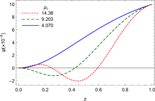
(a) $d=4$, $b=0$

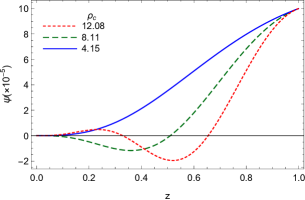
(b) $d=5$, $b=0$

Figure 1: $\psi(z)$ with boundary condition $\psi_{-}=0$ for three lowest values of $\rho_{c}$.

We can determine $\phi$ and $\psi$ by using the numerical calculation. Thus we can find the coefficients in the asymptotic behavior of these fields Eqs.(13) and (14), which are $\mu,\rho$ and $\psi_{+}$(we choose $\psi_{-}$ to be zero). By specifying the values of $\rho$, we can find the resealed critical temperature. In tables (4-3), we summarize the results for the critical temperature of phase transition of holographic superconductor in the presence of logarithmic nonlinear electrodynamics for different values of $b$ and $d$. Also we compare the analytical results obtained from Sturm-Liouville method with those obtained in this subsection numerically. From this table, we observe that the analytical results are in good agreement with the numerical results.

In Table (4) we show the critical temperature for different values of $b$ with the scalar operator $\langle\mathcal{O}\rangle=\langle\mathcal{O_{+}}\rangle$ for 3-dimensional superconductor, we consider $m^{2}=-$2 and $\Delta b=0.1$. We see that the values obtained analytically with this step size, is indeed in very good agreement with the numerical results.

$b$	$\alpha$	$\lambda^{2}_{\rm min}$	$T_{c}\mid_{\rm Analytical}$	$T_{c}\mid_{\rm Numerical}$
$0$	0.601	17.30	0.117$\sqrt{\rho}$	0.118 $\sqrt{\rho}$
$0.1$	0.632	27.79	0.103$\sqrt{\rho}$	0.103$\sqrt{\rho}$
$0.2$	0.652	41.55	0.094$\sqrt{\rho}$	0.092$\sqrt{\rho}$
$0.3$	0.668	61.16	0.085$\sqrt{\rho}$	0.082$\sqrt{\rho}$

Table 1: Critical temperature $T_{c}$ for $d=4$ and $\Delta_{+}=2$, $m^{2}=-2$. Here we choose the step size $\Delta b=0.1$.

Similarly in Table (2) and (3), we show the critical temperature for different values of $b$, of the scalar operator for $4$ and $5$ dimensional superconductor with the mass of scalar field $m^{2}=-3$ and $m^{2}=-4$. We choose the step size $\Delta b=0.1$ and $\Delta b=0.05$. For the case $\Delta b=0.05$, the agreement of analytical results derived from Sturm-Liouville method with the numerical calculation is clearly seen. So by reducing the step size in higher dimensions, we can improve the analytical result.

b		$\alpha_{1}$		$\lambda^{2}_{\rm min(1)}$		$T_{c}|_{\rm Analytical(1)}$		$\alpha_{2}$		$\lambda^{2}_{\rm min(2)}$		$T_{c}|_{\rm Analytical(2)}$		$T_{c}|_{\rm Numerical}$
$0$		0.722		18.23		0.196 $\rho^{1/3}$		0.722		18.23		0.196 $\rho^{1/3}$		0.198$\rho^{1/3}$
$0.1$		0.773		49.25		0.166 $\rho^{1/3}$		0.786		70.38		0.156$\rho^{1/3}$		0.145$\rho^{1/3}$
$0.2$		0.804		126.79		0.142 $\rho^{1/3}$		0.820		251.15		0.126 $\rho^{1/3}$		0.113$\rho^{1/3}$
$0.3$		0.825		327.92		0.121 $\rho^{1/3}$		0.841		942.89		0.101$\rho^{1/3}$		0.090$\rho^{1/3}$

Table 2: Critical temperature $T_{c}$ for $d=5$ and $\Delta_{+}=3,m^{2}=-3$. Here the step size for Analytical(1) is $\Delta b=0.1$ and for Analytical(2) is $\Delta b=0.05$.

b		$\alpha_{1}$		$\lambda^{2}_{\rm min(1)}$		$T_{c}|_{\rm Analytical(1)}$		$\alpha_{2}$		$\lambda^{2}_{\rm min(2)}$		$T_{c}|_{\rm Analytical(2)}$		$T_{c}|_{\rm Numerical}$
$0$		0.792		22.66		0.269 $\rho^{1/4}$		0.792		22.66		0.269 $\rho^{1/4}$		0.271$\rho^{1/4}$
$0.1$		0.854		104.14		0.222 $\rho^{1/4}$		0.878		494.17		0.183$\rho^{1/4}$		0.160$\rho^{1/4}$
$0.2$		0.880		471.19		0.184 $\rho^{1/4}$		0.909		19538.1		0.116 $\rho^{1/4}$		0.104$\rho^{1/4}$
$0.3$		0.902		5283.9		0.136 $\rho^{1/4}$		0.920		1.1$\times 10^{6}$		0.069$\rho^{1/4}$		0.067$\rho^{1/4}$

Table 3: Critical temperature $T_{c}$ for $d=6$ and $\Delta_{+}=4,m^{2}=-4$. Here the step size for Analytical(1) is $\Delta b=0.1$ and for Analytical(2) is $\Delta b=0.05$.

It is worth noting that according to the BF bound given in Eq. (16), the mass of the scalar field, depends on the spacetime dimension. For example, $m^{2}\geq-{9}/{4}$ for $d=4$, $m^{2}\geq-4$ for $d=5$, and $m^{2}\geq-{25}/{4}$ for $d=6$. For convenient, in this paper we choose the mass as $m^{2}=-2,-3,-4$ for $d=4,5,6$, respectively. The reason for these choice comes from the fact that for these values of $m$, the value of $\Delta_{+}$ becomes integer and so the calculations are simplified. In addition, if we assume a fixed value for $m$ in all of these dimensions, we arrive at the same result (see table $4$).

$d$	$\alpha$	$\lambda^{2}_{\rm min}$	$T_{c}\mid_{\rm Analytical}$	$T_{c}\mid_{\rm Numerical}$
$4$	0.601	17.30	0.117$\sqrt{\rho}$	0.118 $\sqrt{\rho}$
$5$	0.786	28.125	0.182$\rho^{1/3}$	0.184$\rho^{1/3}$
$6$	0.848	35.39	0.254$\rho^{1/4}$	0.257$\rho^{1/4}$

Table 4: Critical temperature $T_{c}$ for $b=0$ and $m^{2}=-2$. Here we choose the step size $\Delta b=0.1$.

Therefore, the re-scaled critical temperature increases with increasing the dimension for fixed values of the mass of the scalar field and small values of the nonlinear parameter $b$. From these tables we also understand that for each $d$, the critical temperature decrease as the nonlinear parameter $b$ increases for the fixed scalar field mass. So the condensation gets harder as the nonlinear parameter becomes larger. This result is consistent with the earlier findings [26, 28, 34, 37]. Fig.(2) represents a comparison between these results from numeric and analytic calculations with different values of the step size $\Delta b$.

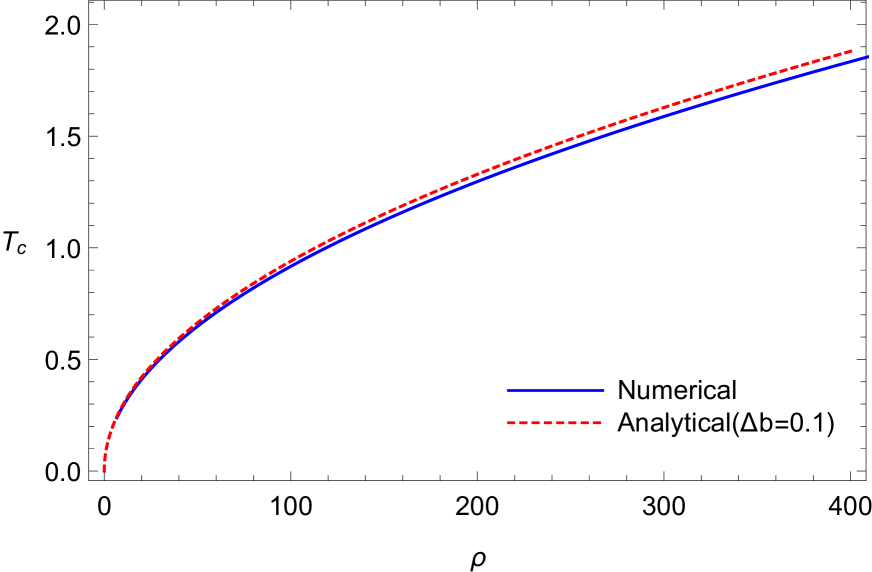
(a)  $d=4,~{}b=0.2$

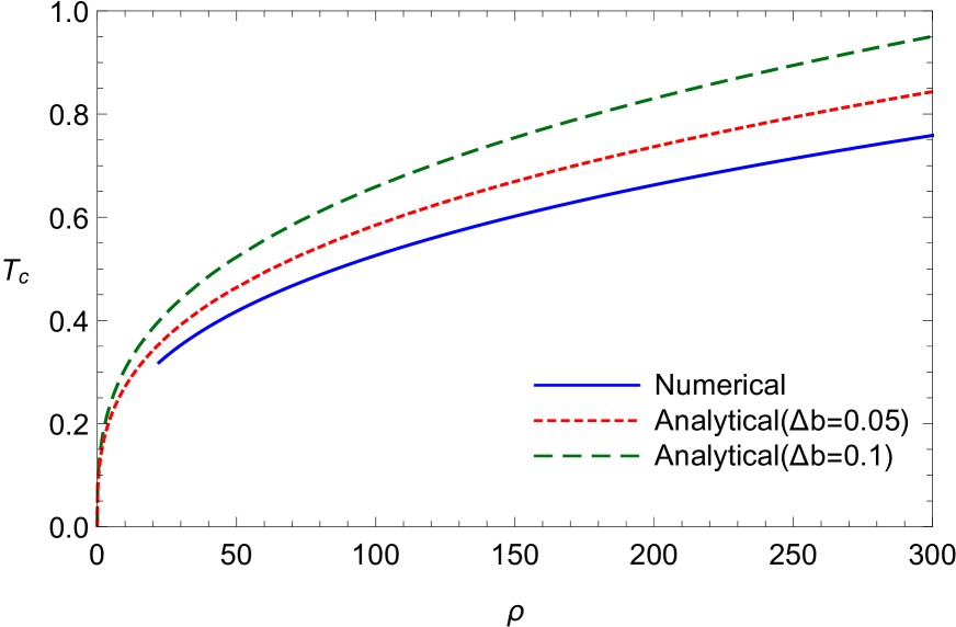
(b)  $d=5,~{}b=0.2$

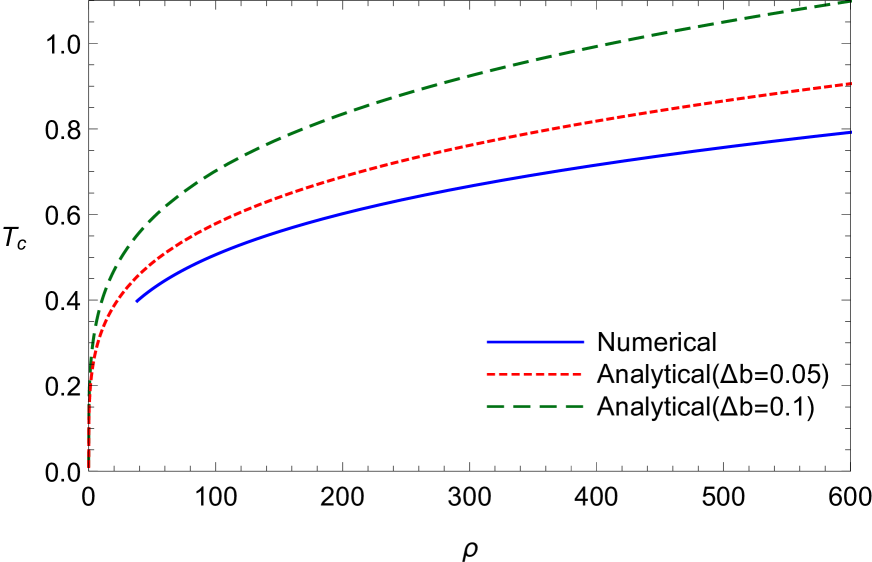
(c)  $d=6,~{}b=0.1$

Figure 2: Comparison of $T_{c}$ in terms of $\rho$ from numerical and analytical calculation.

4 Condensation values and critical exponent

4.1 Analytical method

In this subsection we will calculate the order parameter $\langle\mathcal{O_{+}}\rangle$ as well as the critical exponent in the boundary of spacetime. For this purpose we need the behaviour of the gauge field $\phi$ near the critical point. If we write down Eq.(18) near the critical point $T_{c}$ and keep terms that are linear in $b$, we obtain

$$\phi^{\prime\prime}(z)+\frac{(4-d)}{z}\phi^{\prime}(z)+\frac{(-2+d)z^{3}b\phi^{\prime 3}(z)}{r_{+}^{2}}-2\phi(z)r_{+}^{2}\frac{\psi^{2}(z)}{z^{4}f(z)}\bigg{(}1-\frac{3bz^{4}\phi^{\prime 2}(z)}{2r_{+}^{2}}\bigg{)}=0.$$ (45)

In the previous section we calculate the solution for this equation in the case that we are at the critical point ($\psi=0$), that obtained in the form Eq.(21). Now in this section we consider that the temperature is near the critical temperature, so we have condensation and $\psi\neq 0$, thus we use Eq.(31) for $\psi$. Since we are near to critical point, the condensation value is very small, and we can expand the solution for Eq.(45) around the solution for $\phi$ at $T=T_{c}$ (that we had previously obtained it as Eq.(21)), in terms of small parameter $\frac{\langle\mathcal{O_{+}}\rangle 2}{r_{+}^{2\Delta_{+}}}$, as

$$\frac{\phi(z)}{r_{+}}=\lambda\zeta(z)+\frac{\langle\mathcal{O_{+}}\rangle^{2}}{r_{+}^{2\Delta_{+}}}\chi(z)+\cdot\cdot\cdot~{},$$ (46)

where we have taken the boundary condition as $\chi(1)=\chi^{{}^{\prime}}(1)=0$. Substituting Eq.(31) and (46) into (45), we arrive at the equation for $\chi$

$$\chi^{\prime\prime}(z)+\left[(3d-6)b\lambda^{2}z^{3}\zeta^{\prime 2}(z)+\frac{4-d}{z}\right]\chi^{\prime}(z)=\frac{2z^{-4+2\Delta_{+}}r_{+}^{2}\lambda F^{2}(z)\zeta(z)}{f(z)}\left(1-\frac{3b\lambda^{2}z^{4}\zeta^{\prime 2}(z)}{2}\right).$$ (47)

The left hand side of this equation can be rewritten as

$$\chi^{\prime\prime}(z)+\left[(3d-6)b\lambda^{2}z^{3}\zeta^{\prime 2}(z)+\frac{4-d}{z}\right]\chi^{\prime}(z)=\chi^{\prime\prime}(z)+(3d-12)b\lambda^{2}z^{3}\zeta^{\prime 2}(z)\chi^{\prime}(z)$$

$$+6b\lambda^{2}z^{3}\zeta^{\prime 2}(z)\chi^{\prime}(z)+\frac{4-d}{z}\chi^{\prime}(z).$$ (48)

Taking into account the fact that

$$3b\lambda^{2}z^{4}\zeta^{\prime}(z)\zeta^{\prime\prime}(z)\chi^{\prime}(z)=3b\lambda^{2}z^{4}\zeta^{\prime}(z)\frac{\phi^{\prime\prime}(z)}{\lambda r_{+}}\chi^{\prime}(z),$$ (49)

if we rewrite Eq.(20), we find

$$\phi^{\prime\prime}+\frac{bz^{3}d{\phi^{\prime}}^{3}}{2r_{+}^{2}}\left(1+\frac{bz^{4}}{2r_{+}^{2}}{\phi^{\prime}}^{2}\right)^{-1}+\frac{(4-d)\phi^{\prime}}{z}\left(1+\frac{bz^{4}}{2r_{+}^{2}}{\phi^{\prime}}^{2}\right)^{-1}=0.$$ (50)

and substituting $\phi^{\prime\prime}(z)$ from this into (49), We have,

$$3b\lambda^{2}z^{4}\zeta^{\prime}(z)\zeta^{\prime\prime}(z)\chi^{\prime}(z)=3b\lambda^{2}z^{4}\frac{\zeta^{\prime}(z)}{\lambda r_{+}}\bigg{(}\frac{d-4}{z}\phi^{\prime}+O(b)+O(b^{2})\bigg{)}\chi^{\prime}(z)$$ (51)

$$=3(d-4)b\lambda^{2}z^{3}\zeta^{\prime}\frac{\phi^{\prime}}{\lambda r_{+}}\chi^{\prime}(z)+O(b^{2})+O(b^{3})=3(d-4)b\lambda^{2}z^{3}\zeta^{\prime 2}(z)\chi^{\prime}(z).$$

Therefore we have

$$3(d-4)b\lambda^{2}z^{3}\zeta^{\prime 2}(z)\chi^{\prime}(z)=3b\lambda^{2}z^{4}\zeta^{\prime}(z)\zeta^{\prime\prime}(z)\chi^{\prime}(z),$$ (52)

and hence Eq.(4.1) may be written

$$\chi^{\prime\prime}(z)+3b\lambda^{2}z^{4}\zeta^{\prime}(z)\zeta^{\prime\prime}(z)\chi^{\prime}(z)+6b\lambda^{2}z^{3}\zeta^{\prime 2}(z)\chi^{\prime}(z)+\frac{4-d}{z}\chi^{\prime}(z)$$

$$=\frac{2z^{-4+2\Delta_{+}}r_{+}^{2}\lambda F^{2}(z)\zeta(z)}{f(z)}\left(1-\frac{3b\lambda^{2}z^{4}\zeta^{\prime 2}(z)}{2}\right).$$ (53)

Multiplying both sides of Eq.(4.1) by the following factor,

$$T(z)=\frac{1}{z^{d-4}}e^{\frac{3b\lambda^{2}z^{4}\zeta^{\prime 2}(z)}{2}},$$ (54)

we can write Eq.(4.1) as,

$$(T\chi^{\prime})^{\prime}=\frac{2z^{-d+2\Delta_{+}}r_{+}^{2}\lambda F^{2}(z)\zeta(z)}{f(z)}.$$ (55)

Integrating the above equation in the interval $[0,1]$ and using the boundary conditions for $\chi$, yields

$$T(z)\chi^{\prime}(z)|_{z\rightarrow 0}=-\int_{0}^{1}\frac{2z^{-d+2\Delta_{+}}r_{+}^{2}\lambda F^{2}(z)\zeta(z)}{f(z)}dz.$$ (56)

Substituting $T(z)$ in above equation and noting that we have two cases for $\zeta(z)$ to substitute in this equation, we finally obtain

$$\left[\frac{\chi^{\prime}(z)}{z^{d-4}}\right]\bigg{|}_{z\rightarrow 0}=-\lambda\mathcal{A},$$ (57)

$$\mathcal{A}=\left\{\begin{array}[]{rl}\mathcal{A}_{1}{}{}{}{}{}{}&\quad\mathrm{for}\ 2(d-3)^{2}b_{n}(\lambda^{2}|_{b_{n-1}})<1,\\ &\\ (\mathcal{A}_{2}+\mathcal{A}_{3})\ ,&\quad\mathrm{for}\ 2(d-3)^{2}b_{n}(\lambda^{2}|_{b_{n-1}})>1,\end{array}\right.$$ (61)

where

$$\mathcal{A}_{1}=\int_{0}^{1}\frac{2r_{+}^{2}z^{2\Delta_{+}-d}F^{2}\zeta_{1}}{f}dz,~{}~{}\mathcal{A}_{2}=\int_{0}^{z_{0}}\frac{2r_{+}^{2}z^{2\Delta_{+}-d}F^{2}\zeta_{2}}{f}dz,~{}\mathcal{A}_{3}=\int_{z_{0}}^{1}\frac{2r_{+}^{2}z^{2\Delta_{+}-d}F^{2}\zeta_{3}}{f}dz,$$ (62)

where $\zeta_{1}$, $\zeta_{2}$ and $\zeta_{3}$ are given by Eqs.(25), (26) and (29). Now we write down the relation between $\chi^{\prime}(z)$ and $(d-3)$-th derivative of $\chi(z)$. If we rewrite Eq.(47) at $z\rightarrow 0$, we have

$$\chi^{\prime\prime}(0)=\chi^{\prime}\left(\frac{d-4}{z}\right)\big{|}_{z\rightarrow 0},$$ (63)

thus is a matter of calculations to show that we can write the following relation in $d$-dimensions,

$$\frac{\chi^{(d-3)}(z=0)}{(d-4)!}=\frac{\chi^{\prime}}{z^{d-4}}\big{|}_{z\rightarrow 0}.$$ (64)

From Eqs.(13) and (46) and by expanding $\chi(z)$ around $z=0$, we have

$$\mu-\frac{\rho}{r_{+}^{d-3}}z^{d-3}=r_{+}\lambda\zeta+\frac{\langle\mathcal{O_{+}}\rangle^{2}}{r_{+}^{2\Delta_{+}-1}}~{}\Bigg{\{}\chi(0)+z\chi^{\prime}(0)+...+z^{(d-3)}\frac{\chi^{(d-3)}(0)}{(d-3)!}+...\Bigg{\}}.$$ (65)

Comparing the coefficient of $z^{d-3}$ on both sides of the above equation we obtain

$$-\frac{\rho}{r_{+}^{d-2}}=-\lambda+\frac{\langle\mathcal{O_{+}}\rangle^{2}}{r_{+}^{2\Delta_{+}}}~{}\frac{\chi^{d-3}(0)}{(d-3)!}~{},$$ (66)

Using Eq.(66) and (57), we arrive at

$$\frac{\rho}{r_{+}^{d-2}}=\lambda\left[1+\frac{\langle\mathcal{O_{+}}\rangle^{2}}{r_{+}^{2\Delta_{+}}}\frac{\mathcal{A}}{(d-3)}\right],$$ (67)

with regards to definition of $\lambda=\frac{\rho}{r_{+c}^{d-2}}$, and substituting $r_{+}$ and $r_{+c}$ from the relations that we have for $T$ and $T_{c}$ given in Eqs.(8) and (38), we find the relation between the condensation operator and the critical temperature in $d$-dimensional spacetime near the critical temperature ($T\sim T_{c}$) as

$$\langle\mathcal{O_{+}}\rangle=\left(\frac{4\pi}{d-1}\right)^{\Delta_{+}}\sqrt{\frac{(d-3)(d-2)}{\mathcal{A}}}~{}T_{c}^{\Delta_{+}}\sqrt{1-\frac{T}{T_{c}}}.$$ (68)

Thus, we find that the critical exponent of the order parameter is $1/2$, and near the critical point this operator satisfies

$$\langle\mathcal{O_{+}}\rangle=\beta T_{c}^{\Delta_{+}}\left(1-\frac{T}{T_{c}}\right)^{{1}/{2}},$$ (69)

which holds for various values of $b$, $m$ and $d$. The coefficient $\beta$ is given by

$$\beta=\left\{\begin{array}[]{rl}\left(\frac{4\pi}{d-1}\right)^{\Delta_{+}}\sqrt{\frac{(d-3)(d-2)}{\mathcal{A}_{1}}}\ ,{}{}{}{}&\quad\mathrm{for}\ 2(d-3)^{2}b_{n}(\lambda^{2}|_{b_{n-1}})<1,\\ &\\ \left(\frac{4\pi}{d-1}\right)^{\Delta_{+}}\sqrt{\frac{(d-3)(d-2)}{\mathcal{A}_{2}+\mathcal{A}_{3}}}\ ,&\quad\mathrm{for}\ 2(d-3)^{2}b_{n}(\lambda^{2}|_{b_{n-1}})>1.\end{array}\right.$$ (73)

From these results we can analysis the effect of the nonlinear parameter $b$ and the spacetime dimension $d$, on the values of $\beta$. Our analytical results are presented in table (5),(6) and (7) which we also compare them with the numerical results.

4.2 Numerical method

In the previous section for the numerical solution, we was needed only the charge density at the critical point for obtaining the re-scaled critical temperature. Here we start with increasing $\psi(1)$ from $\psi(1)=\frac{1}{10000}$ to higher values in the small steps, meaning that the temperature becomes lower. At any step we can find all the coefficient of the asymptotic behavior of $\psi$ and $\phi$, such as $\psi_{+}$. We use the value of $\psi_{+}$ for calculation of the order parameter $\langle\mathcal{O_{+}}\rangle$, and exploring the behavior of this parameter in terms of temperature for different dimension of the spacetime and for different values of $b$. For example for $d=4,5,6$ we obtain condensation $\langle\mathcal{O_{+}}\rangle$ from following relations,

$$\langle\mathcal{O_{+}}\rangle = \sqrt{2}\psi_{+}\quad\mathrm{for}~{}~{}d=4,$$ (74)

$$\langle\mathcal{O_{+}}\rangle = \psi_{+}\quad~{}~{}~{}~{}\mathrm{for}~{}~{}~{}d=5,6,$$ (75)

where the coefficient $\sqrt{2}$ is a convenient normalization factor [3]. Now we want to plot the dimensionless condensation as a function of dimensionless temperature. Since we work in units where $c=\hbar=1$, all physical quantities can be described in unit which is some power of the mass. In this unit, length and time have dimension of $[mass]^{-1}$, energy, momentum and $T$ have dimension $[mass]$, while $\rho$ has dimension $[mass]^{d-2}$. Also since in this unit, the scalar field must be dimensionless, so $\psi_{+}$ must have dimension $[mass]^{\Delta_{+}}$.
Thus we can plot dimensionless ${\langle\mathcal{O_{+}}\rangle}/{T_{c}^{\Delta_{+}}}$ as a function of ${T}/{T_{c}}$, where $\Delta_{+}$ is defined by Eq.(15).

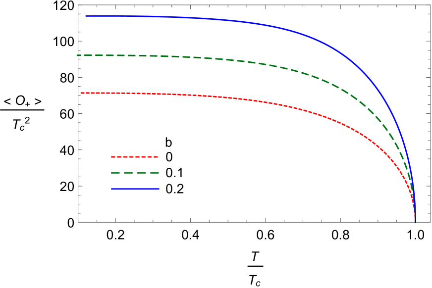
(a)  $d=4$

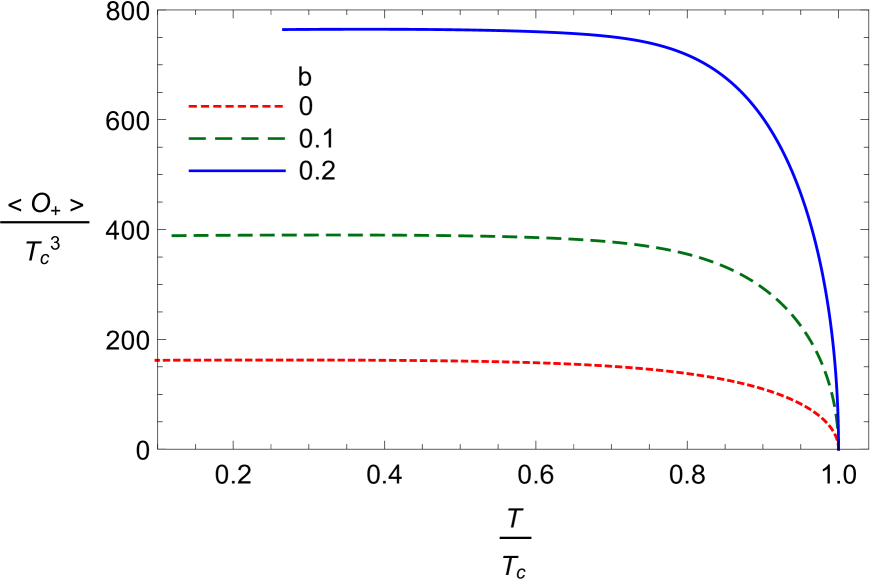
(b)  $d=5$

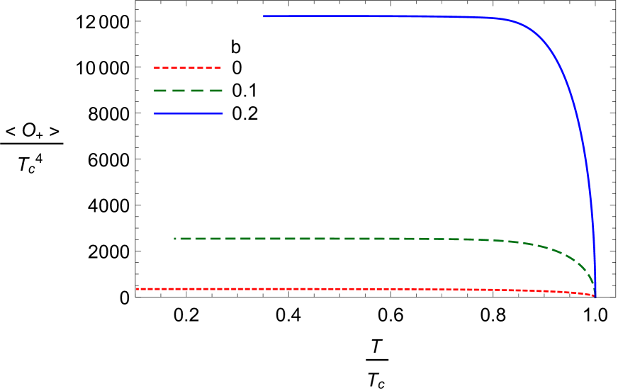
(c)  $d=6$

Figure 3: The dimensionless condensation operator in terms of dimension less temperature for different values of $b$.

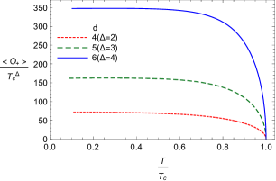
(a) $b=0$

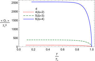
(b) $b=0.1$

Figure 4: The dimensionless condensation operator in terms of dimensionless temperature for different values of $d$.

This curves for the condensation operator are qualitatively similar to what that obtained in BCS theory, the condensate rises quickly when the system is stayed on below the critical temperature and goes to a constant as $T\rightarrow 0$. Near the critical temperature, as obtained from analytical results in Eq.(69), the condensate is proportional to $(1-\frac{T}{T_{c}})^{1/2}$, that is the behavior that predicted by Landau-Ginzburg theory. This curves for $d=4,5,6$ in Fig.(3) represents that, when we increase $b$, the dimensionless condensation becomes larger. Also, by comparing the condensation for different $d$ in Fig.(4), we find that it becomes large in higher dimensions.

Now we find that the results obtained for the behaviour of the condensation operator near the critical point, from numerical calculation is in good agreement with the results obtained from analytical calculation in Eq.(69). From Eq.(69) we can write

$$\ln\left(\frac{\langle\mathcal{O_{+}}\rangle}{T_{c}^{\Delta_{+}}}\right)=\ln\beta+\frac{1}{2}\ln\left(1-\frac{T}{T_{c}}\right),$$ (76)

Now we can plot $\ln\left(\frac{\langle\mathcal{O_{+}}\rangle}{T_{c}^{\Delta_{+}}}\right)$ as a function of $\ln(1-\frac{T}{T_{c}})$. From the dotted curves in Fig.(5), we see that the plot which is fitted to a straight line has slop $1/2$, that is the critical exponent. The slope is independent of parameters $b$ and $d$. Also we can find $\beta$ from the y-intercept of the lines. Finally we conclude that the phase transition is of second order and the critical exponent of the system always take the value $1/2$, and the nonlinear electrodynamics can not change the result. This result seems to be a universal property for various nonlinear electrodynamics [27, 34, 29].

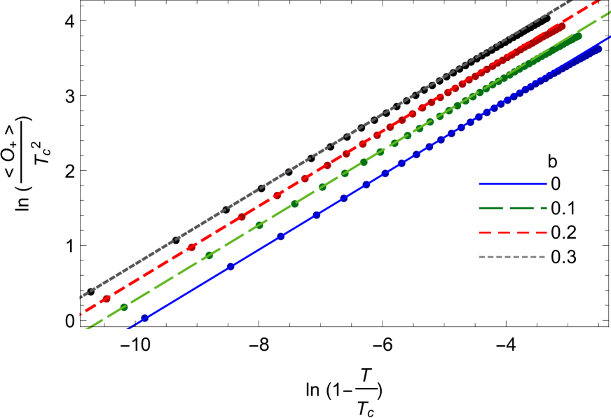
(a)  $d=4$

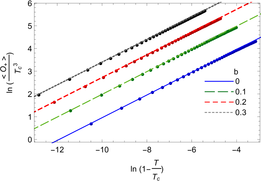
(b)  $d=5$

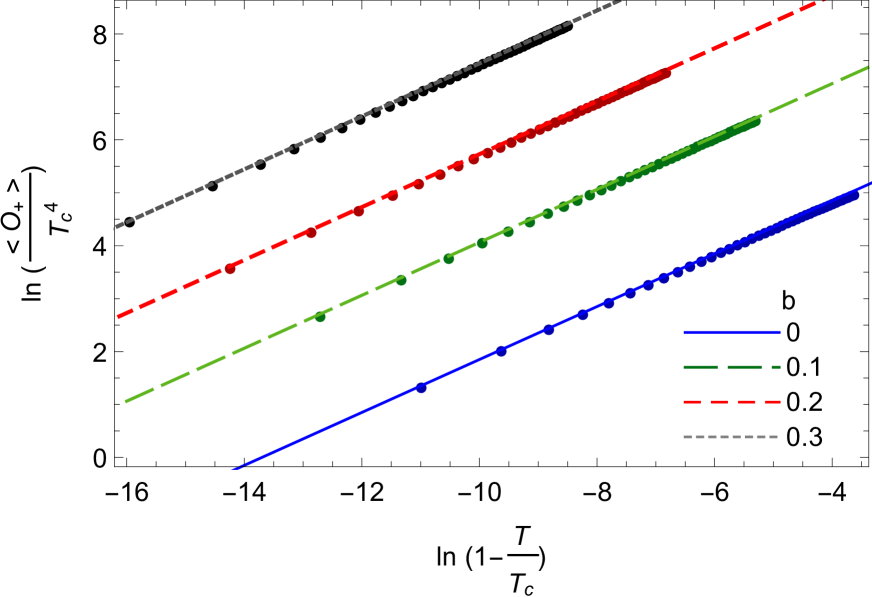
(c)  $d=6$

Figure 5: Fitting the order parameter with a straight line whose slope is ${1}/{2}$ for different $b$ and $d$.

Now we summarize the results for $\beta$ for a holographic superconductor in logarithmic electrodynamics, which obtained from analytical calculation from Eq.(73) and from numerical calculation which explained before, for different values of $b$ and $d$, in tables (5),(6) and (7). Also we compare these results.

b		$\gamma|_{\rm Analytical}$		$\gamma|_{\rm Numerical}$
0		92.8		140.09
0.1		108.88		194.52
0.2		124.03		251.09
0.3		282.83		314.32

Table 5: The values of $\gamma=\sqrt{2}\beta$ for $d=4$ and the step size $\Delta b=0.1$.

The results that obtained for $\beta$ from the numerical and analytical solutions for $d=5$ and $d=6$ represent in the last tables. Also for these dimensions, the results from analytical for the step size $\Delta b=0.1$ is far from the numerical, so we consider a smaller step size $\Delta b=0.05$, to increase our accuracy.

b		$\beta|_{\rm Analytical(1)}$		$\beta|_{\rm Analytical(2)}$		$\beta|_{\rm Numerical}$
0		238.5		238.5		385.20
0.1		330.93		369.70		1077.9
0.2		441.06		537.81		2259.4
0.3		580.26		779.34		4445.8

Table 6: The values of $\beta$ for $d=5$ and the step size for Analytical(1) is $\Delta b=0.1$ and for Analytical(2) $\Delta b=0.05$.

b		$\beta|_{\rm Analytical(1)}$		$\beta|_{\rm Analytical(2)}$		$\beta|_{\rm Numerical}$
0		533.82		533.82		934.97
0.1		871.26		1088.12		8629.5
0.2		1350.20		2920.86		45677
0.3		2071.40		8213.86		253670

Table 7: The values of $\beta$ for $d=6$ and the step size for Analytical (1) is $\Delta b=0.1$ and for Analytical(2) $\Delta b=0.05$.

From these tables we find that the value $\beta$, increases with increasing the nonlinear parameter $b$. Also, when the step size $\Delta b$ is smaller, the analytical results are closer with the numerical results rather than the larger step size.

5 Conductivity

The superconductor energy gap is an essential feature of the superconducting state which may be characterized by the threshold frequency obtained from the electrical conductivity. Hence, in this section we investigate the behavior of the electric conductivity as a function of frequency. In the linear response theory, the conductivity is expressed as the current density response to an applied electric field

$$\sigma_{ij}=\frac{J_{i}}{E_{j}}~{}.$$ (77)

According to the AdS/CFT correspondence dictionary, if we want to have current in the boundary, we must consider a vector potential in the bulk. This implies that by solving for fluctuations of the vector potential $A_{j}$ in the bulk, we will have a dual current operator $J_{i}$ in the CFT [3]. Inasmuch as the dual CFT has a spatial symmetry, one can consider just the conductivity in the $x$ direction. We turn on the small perturbation in the bulk gauge potential as

$$\delta A_{x}=A_{x}(r)e^{-i\omega t}~{},$$

where $\omega$ is the frequency. Thus, the equation of motion for $A_{x}(r)$, at the linearized level of the perturbation, takes the form

$$\big{(}2-b\phi^{\prime 2}(r)\big{)}A_{x}^{\prime\prime}(r)+\bigg{[}2b\phi^{\prime}(r)\phi^{\prime\prime}(r)+\left(\frac{d-4}{r}+\frac{f^{\prime}(r)}{f(r)}\right)\big{(}2-b\phi^{\prime 2}(r)\big{)}\bigg{]}A_{x}^{\prime}(r)$$

$$+\frac{\omega^{2}}{f^{2}(r)}\big{(}2-b\phi^{\prime 2}(r)\big{)}A_{x}(r)-\frac{\psi^{2}(r)}{f(r)}(2-b\phi^{\prime 2}(r))^{2}A_{x}(r)=0.$$ (78)

The asymptotic ($r\rightarrow\infty$) behavior of the above differential equation is obtained as

$$A_{x}^{\prime\prime}(r)+\frac{d-2}{r}A_{x}^{\prime}(r)+\frac{\omega^{2}}{r^{4}}A_{x}(r)=0,$$

which admits the following solution in the asymptotic $(r\rightarrow\infty)$,

$$A_{x}=\left\{\begin{array}[]{rl}A^{(0)}+\frac{A^{(1)}}{r}-\frac{\omega^{2}A^{(0)}}{2r^{2}}...\ ,&\ \ ~{}~{}\mathrm{for}\ d=4,\\ &\\ A^{(0)}+\frac{A^{(1)}}{r^{2}}+\frac{\omega^{2}A^{(0)}ln(kr)}{2r^{2}}+...,&\ \quad\mathrm{for}\ d=5,\\ &\\ A^{(0)}+\frac{A^{(1)}}{r^{3}}+\frac{\omega^{2}A^{(0)}}{2r^{2}}...\ ,&\ \ ~{}~{}\mathrm{for}\ d=6,\\ &\\ \end{array}\right.$$ (79)

where $A^{(0)},A^{(1)}$ are constant parameters and $k$ is a constant with $[\textit{length}]^{-1}$ dimension which inserted for a dimensionless logarithmic argument. From the AdS/CFT dictionary, the boundary current operator may be calculated by differentiating the action [43]

$$J=\frac{\delta S_{bulk}}{\delta A^{(0)}}=\frac{\delta S_{o.s}}{\delta A^{(0)}}=\frac{\partial\left(\sqrt{-g}\mathcal{L}_{m}\right)}{\partial A_{x}^{{}^{\prime}}}~{}\big{|}_{r\rightarrow\infty},$$ (80)

where $A^{(0)}$ is the dual to a source in the boundary theory. Also, $S_{o.s}$ and $\mathcal{L}_{m}$ are, respectively, the on-shell bulk action and the Lagrangian of the matter field. The $S_{o.s}$ action is given by

$$S_{o.s}=\int_{r_{+}}^{\infty}dr\int d^{d-1}x\sqrt{-g}\mathcal{L}_{m}.$$ (81)

Expanding the action to quadratic order in the perturbation and taking into account Eq.(78), $S_{o.s.}$ reduces to

$$S_{o.s}=\int d^{d-1}x~{}\frac{r^{d-4}f(r)A_{x}(r)A_{x}^{\prime}(r)}{-2+b\phi^{\prime 2}(r)}\big{|}_{r\rightarrow\infty}.$$ (82)

According to the asymptotic behavior of $\phi$ and $A_{x}$ given by Eq.(13) and Eq.(79), and using Eq.(80), one can calculate the holographic current as

$$J_{x}=\left\{\begin{array}[]{rl}A^{(1)}\ ,&\ \ ~{}~{}\mathrm{for}\ d=4\\ &\\ 2A^{(1)}-\frac{\omega^{2}A^{(0)}}{2},&\ \quad\mathrm{for}\ d=5,\\ &\\ 3A^{(1)}\ ,&\ \ ~{}~{}\mathrm{for}\ d=6.\\ &\\ \end{array}\right.$$ (83)

Thus, from Eq. (77) and $E_{x}=-\partial_{t}\delta A_{x}$, the electrical conductivity is obtained as

$$\sigma=\left\{\begin{array}[]{rl}\frac{A^{(1)}}{i\omega A^{(0)}}\ ,&\ \ ~{}~{}\mathrm{for}\ d=4,\\ &\\ \frac{2A^{(1)}}{i\omega A^{(0)}}+\frac{i\omega}{2},&\ \quad\mathrm{for}\ d=5,\\ &\\ \frac{3A^{(1)}}{i\omega A^{(0)}}\ ,&\ \ ~{}~{}\mathrm{for}\ d=6.\\ &\\ \end{array}\right.$$ (84)

It is worth noting that the divergence terms in the above action is eliminated by adding a suitable counterterm [44],[16]. Now, one can numerically solve the differential equation for $A_{x}(r)$ in Eq.(78) by imposing an ingoing wave boundary condition near the event horizon [7]

$$A_{x}(r)=S(r)f^{{-i\omega}/{(4\pi T)}},$$ (85)

where

$$S(r)=1+a_{1}(r-r_{+})+a_{2}(r-r_{+})^{2}+...,$$

$T$ is the Hawking temperature and the coefficients $a_{1}$, $a_{2}$, $\ldots$ are characterized by Taylor expansion of Eq.(78) around the horizon $r_{+}$. With $A_{x}$ at hand, we can calculate the conductivity from Eq.(84). We summarize our results regarding the behaviour of the conductivity in Figs.(6-9).

The behavior of the real parts of conductivity as a function of frequency for various nonlinear parameter $b$ and in various dimension at different temperature are depicted in Fig.(6). As one can see from this figure, the superconducting gap appears below the critical temperature that becomes deep with decreasing the temperature. That means $\omega_{g}$ becomes larger. Since $\omega_{g}$ is probational to the minimum energy that needed to break the condensation, therefore with decreasing the temperature, the condensation becomes stronger. Also, the gap becomes sharper as we decrease the temperature. At enough large frequency, the behavior of conductivity indicates a normal state that follows a power law relation with frequency, i.e. $\mathrm{Re}[\sigma]\varpropto\omega^{d-4}$ [43]. For $3$-dimension of CFT, the real part of conductivity is independent of frequency which tends toward a constant value for large frequency (see Figs.6(a) and 6(b)).

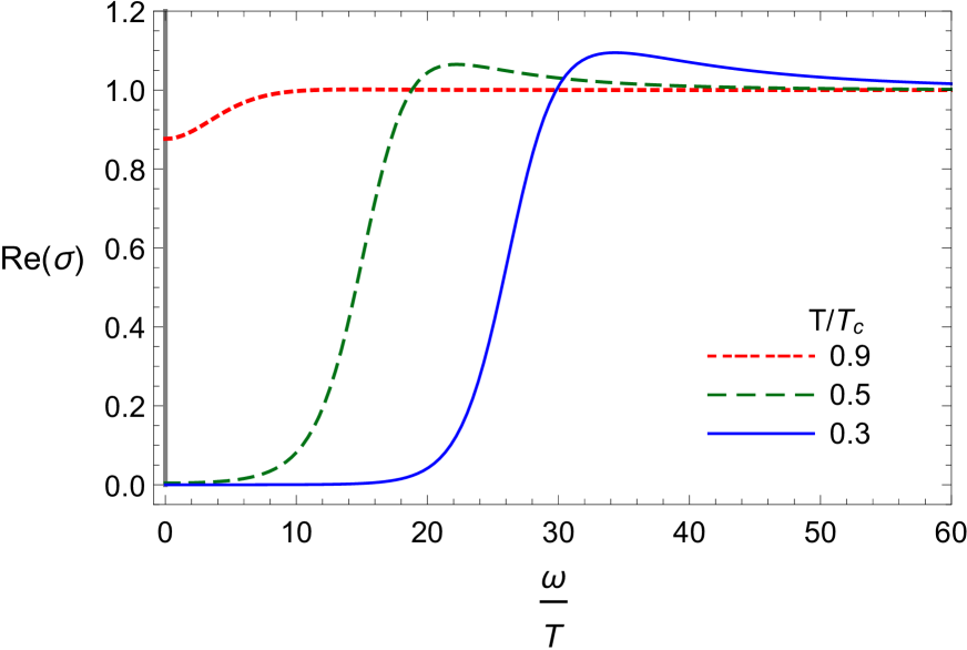
(a)  $d=4,~{}b=0$

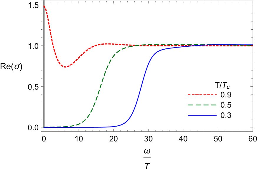
(b)  $d=4,~{}b=0.1$

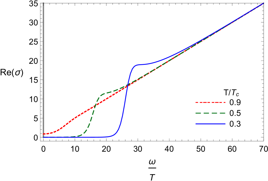
(c)  $d=5,~{}b=0$

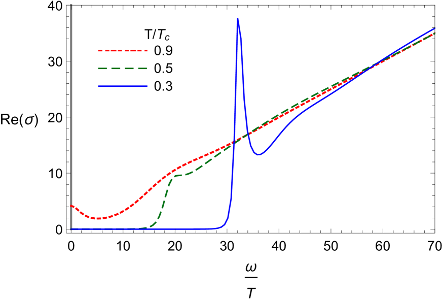
(d) $~{}d=5,~{}b=0.1$

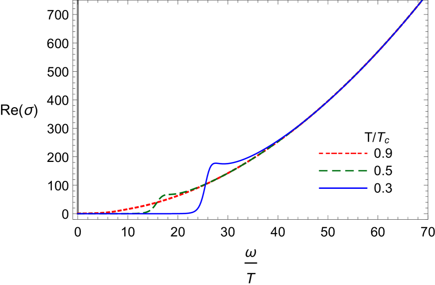
(e) $~{}d=6,~{}b=0$

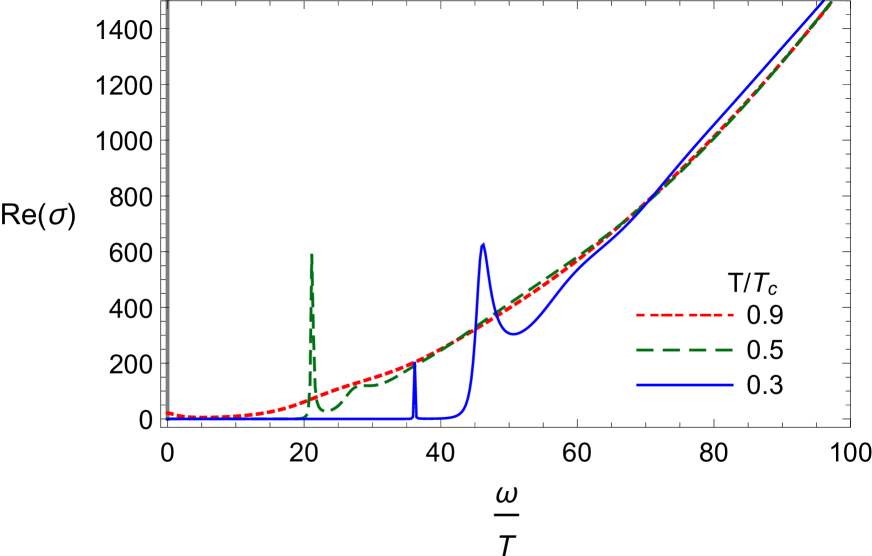
(f) $~{}d=6,~{}b=0.1$

Figure 6: The real part of conductivity for different temperature in terms of $\omega/T$.

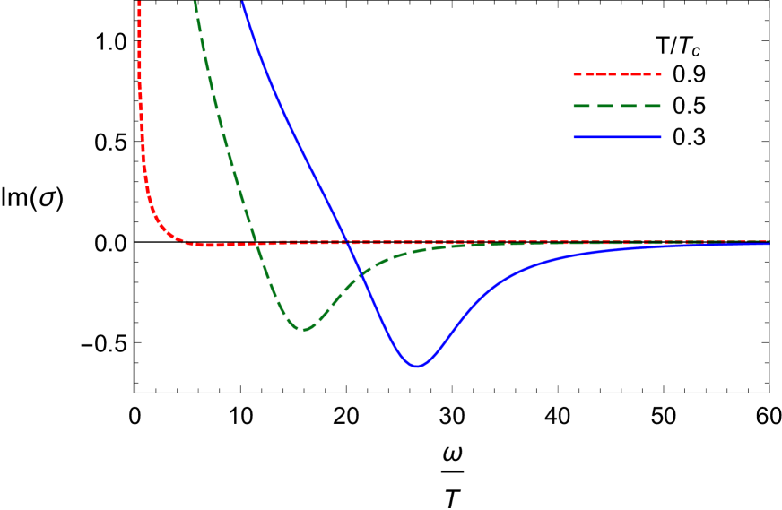
(a)  $d=4,~{}b=0$

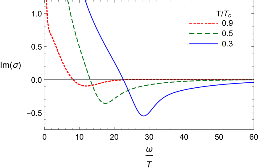
(b)  $d=4,~{}b=0.1$

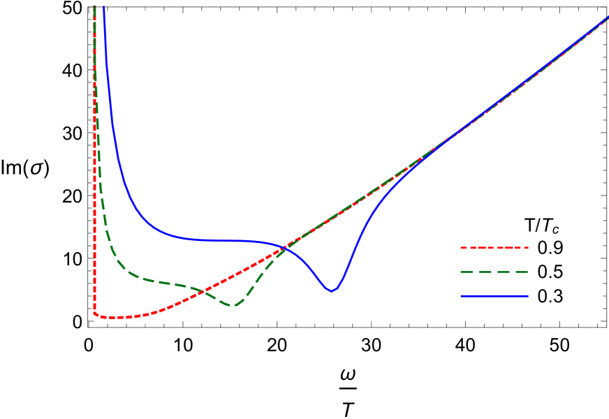
(c)  $d=5,~{}b=0$

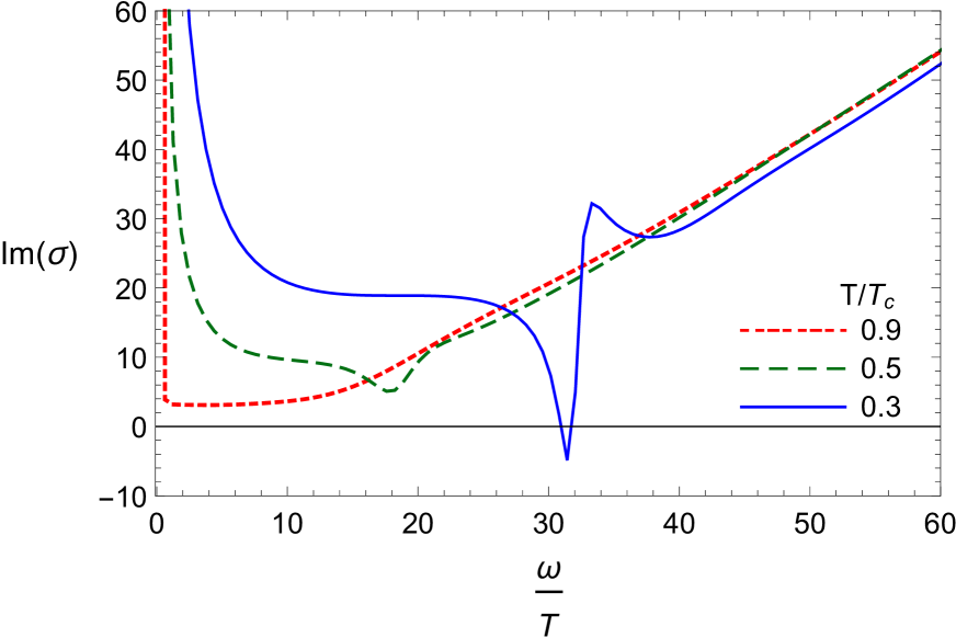
(d) $~{}d=5,~{}b=0.1$

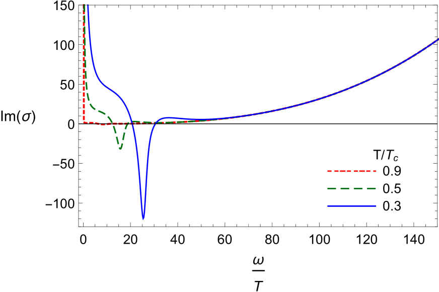
(e) $~{}d=6,~{}b=0$

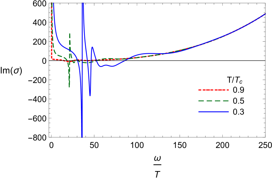
(f) $~{}d=6,~{}b=0.1$

Figure 7: The imaginary part of conductivity for different temperature in terms of $\omega/T$.

The associated imaginary parts of conductivity are illustrated in Fig. 7 which is related to the real parts of conductivity by the Kramers–Kronig relations. Hence, the pole in the imaginary parts of conductivity at $\omega=0$ points out to a delta function in the real parts which are shown by the vertical lines in Fig. 6. Although, the delta function cannot be resolved numerically, but we know that it exists. By comparison the figures, we find that at any fixed temperature and frequency, the conductivity in higher dimensions is larger. For $d=6$, more delta functions and poles appear inside the gap as one decreases the temperature. The BCS theory explains systems that are weak coupled, which means, there was no interaction between the pairs. But holographic superconductors are strongly coupled. With decreasing the temperature, the interactions become stronger and form a bound state. The additional delta functions and poles related to this state [8].

In order to determine the effect of the dimension and nonlinear parameter on the superconducting gap at low temperature $T\approx 0.15T_{c}$, we plot real and imaginary parts of the holographic electrical conductivity as a function of normalized frequency $\omega/T_{c}$ in Figs.8 and 9. From the BCS theory we have relation $\omega_{g}=2\Delta$, where $\Delta$ is the energy required for charged excitations, that leads to $\omega_{g}\simeq 3.5T_{c}$. In [8], it was shown that the relation connecting the frequency gap with the critical temperature, for $d=3$ and $d=4$ dimensional holographic superconductor becomes ${\omega_{g}}/{T_{c}}\approx 8$, which is more than twice of the corresponding value in the BCS theory. Also it was argued that this ratio for $d=4,5$, is always about eight, and the relation $\omega_{g}/T_{c}\approx 8$ is universal. However, as one can see from Fig.8 in each dimension, the superconducting gap increases with increasing the nonlinear parameter $b$. Also, for the fixed value of the nonlinear parameter $b$, the energy gap effectively increases with increasing the dimension, which indicates that the holographic superconductor state is destroyed for large $\omega/T_{c}$. This implies that the relation between $\omega_{g}$ and $T_{c}$ depends on the parameters $b$ and $d$.

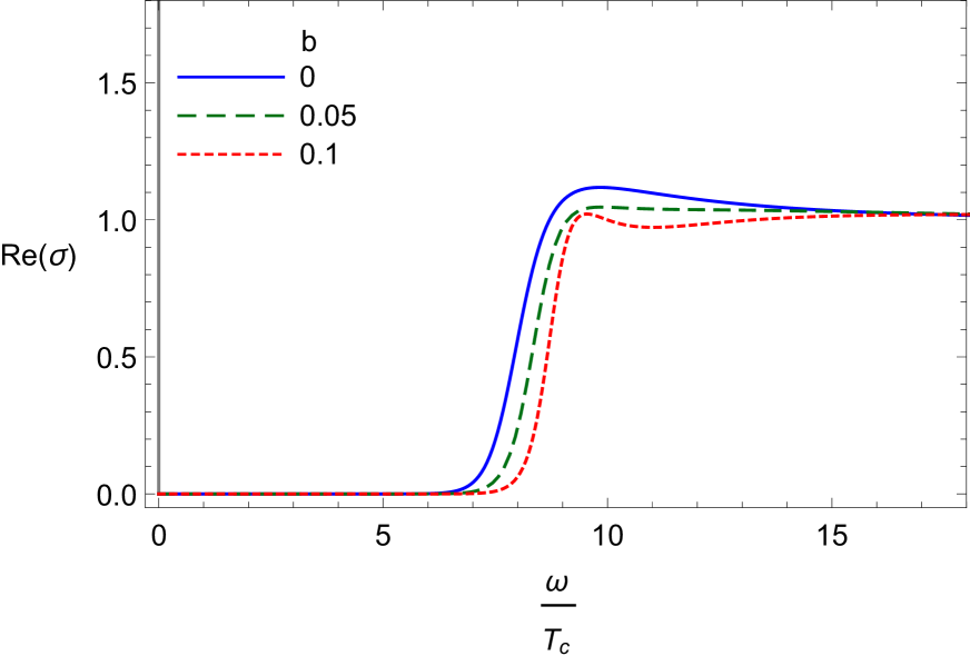
(a) $~{}d=4,~{}T/T_{c}\approx 0.15$

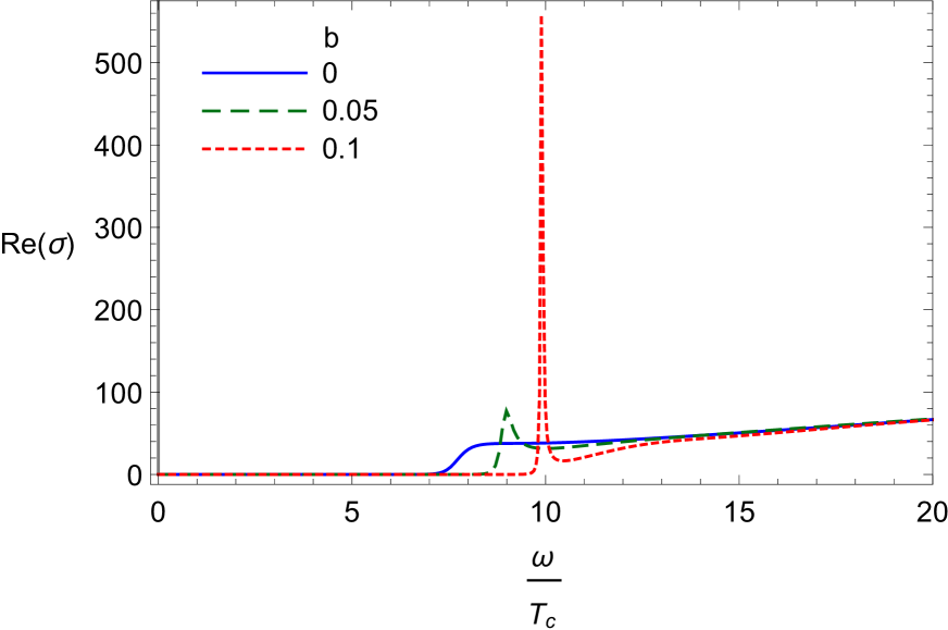
(b) $~{}d=5,~{}T/T_{c}\approx 0.15$

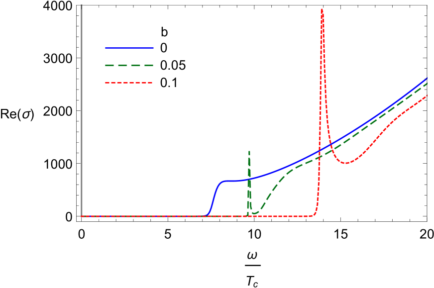
(c) $~{}d=6,~{}T/T_{c}\approx 0.15$

Figure 8: The real part of conductivity for different $b$ in terms of $\omega/T_{c}$.

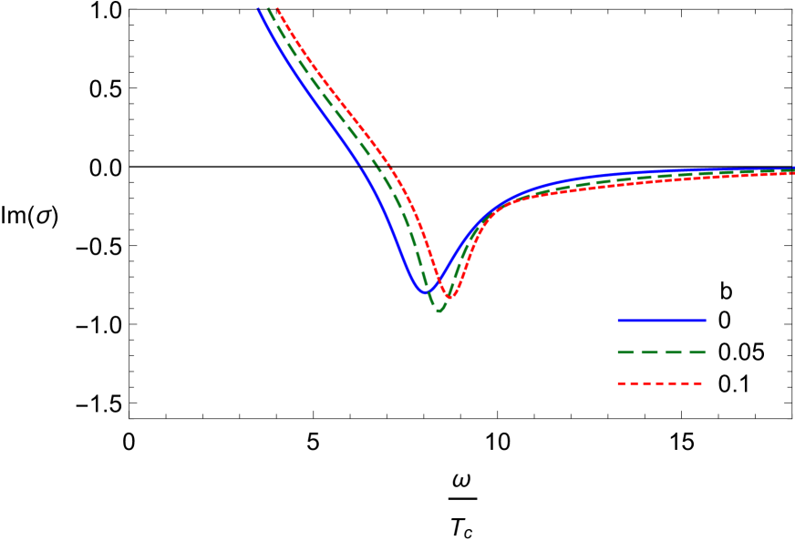
(a) $~{}d=4$

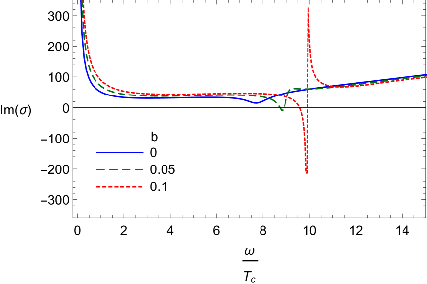
(b) $~{}d=5$

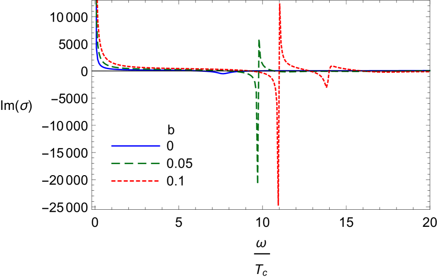
(c) $~{}d=6$

Figure 9: The real part of conductivity for different $b$ in terms of $\omega/T_{c}$.

6 Closing Remarks

To sum up, in this paper we have continued the study on the gauge/gravity duality by investigating the properties of the $s$-wave holographic superconductor in higher dimensional spacetime and in the presence of nonlinear gauge field. We have considered the Logarithmic Lagrangian for the $U(1)$ gauge theory which was proposed by Soleng [42]. We follow the Sturm-Liouville eigenvalue problem for our analytical study as well as the numerical shooting method. We explored three aspects of these kinds of superconductors. First, we obtained the relation between critical temperature and charge density, $\rho$, and disclosed the effects of both nonlinear parameter $b$ and the dimensions of spacetime, $d$, on the critical temperature $T_{c}$. We found that in each dimension, $T_{c}/{\rho}^{1/(d-2)}$ decreases with increasing the nonlinear parameter $b$. Besides, for a fixed value of $b$, this ratio increases for the higher dimensional spacetime. This implies that the high temperature superconductor can be achieved in the higher dimensional spacetime. We confirmed that our analytical method is in good agreement with the numerical results. Second, we have calculated the condensation value and critical exponent of the system analytically as well as numerically and observed that in each dimension, the coefficient $\beta$ becomes larger with increasing the nonlinear parameter $b$. Besides, for a fixed value of $b$, it increases with increasing the spacetime dimension, i.e., in higher dimensional spacetime.

Finally, we explored the electrical conductivity of the holographic superconductor. Our aim in this part was to disclose the effects of the nonlinear gauge field as well as the higher dimensional spacetime on the superconducting gap of the holographic superconductor. We observed that the superconducting gap appears below the critical temperature that becomes deep with decreasing the temperature. Besides, we found that at high frequency, the behavior of conductivity indicates a normal state that follows a power law relation with frequency, i.e. $\mathrm{Re}[\sigma]\varpropto\omega^{d-4}$. We also investigated the imaginary part of superconductor and found that the pole in the imaginary parts of conductivity at $\omega=0$ points out to a delta function in the real parts. We concluded that for a fixed value of the nonlinear parameter $b$, the energy of gap effectively increases with increasing the dimension, which indicates that the holographic superconductor state is destroyed for large $\omega/T_{c}$. This indicates that the relation between $\omega_{g}$ and $T_{c}$ depends on the parameters $b$ and $d$.

References

- [1] J. Bardeen, L. N. Cooper, J. R. Schrieer, Theory of Superconductivity, Phys. Rev. 108, 1175 (1957).
- [2] J. Maldacena, The large N limit of superconformal eld theories and supergravity, Adv. Theor. Math. Phys. 2, 231 (1998), [arXiv:9711200].
- [3] S. A. Hartnoll, C. P. Herzog and G. T. Horowitz, Building a Holographic Superconductor, Phys. Rev. Lett. 101, 031601 (2008), [arXiv:0803.3295].
- [4] S. A. Hartnoll, C. P. Herzog and G. T. Horowitz, Holographic Superconductors, JHEP 12, 015 (2008), [arXiv:0810.1563].
- [5] S.S. Gubser, Breaking an Abelian gauge symmetry near a black hole horizon, Phys. Rev. D 78, 065034 (2008), [arXiv:0801.2977].
- [6] C.P. Herzog, Lectures on holographic superfluidity and superconductivity, J. Phys. A 42, 343001 (2009).
- [7] S.A. Hartnoll, Lectures on holographic methods for condensed matter physics, Class. Quantum Grav. 26, 224002 (2009).
- [8] G.T. Horowitz and M.M. Roberts, Holographic Superconductors with Various Condensates, Phys. Rev. D 78, 126008 (2008)
- [9] G. T. Horowitz, Introduction to Holographic Superconductors, Lect. Notes Phys. 828, 313 (2011), [arXiv:1002.1722 [hepth]].
- [10] Q. Pan, J. Jing, B. Wang, S. Chen, Analytical study on holographic superconductors with backreactions, JHEP 06, 087 (2012) [arXiv:1205.3543].
- [11] H. B. Zeng, X. Gao, Y. Jiang, and H. S. Zong, Analytical computation of critical exponents in several holographic superconductors, JHEP 1105, 002 (2011), [arXiv:1012.5564].
- [12] R. G. Cai, H. F Li, H.Q. Zhang, Analytical studies on holographic insulator/superconductor phase transitions, Phys. Rev. D 83, 126007 (2011), [arXiv:1103.5568].
- [13] Q. Pan, B. Wang, E. Papantonopoulos, J. Oliveira, A. B. Pavan, Holographic superconductors with various condensates in Einstein-Gauss-Bonnet gravity, Phys. Rev. D 81, 106007 (2010), [arXiv:0912.2475].
- [14] Q. Pan, B. Wang, General holographic superconductor models with Gauss-Bonnet corrections, Phys. Lett. B 693 159 (2010), [arXiv:1005.4743].
- [15] H. F. Li, R. G. Cai, H. Q. Zhang, Analytical studies on holographic superconductors in Gauss-Bonnet gravity, JHEP 04, 028 (2011), [arXiv:1103.2833].
- [16] L. Barclay, R. Gregory, S. Kanno, P. Sutcliffe, Gauss-Bonnet holographic superconductors, JHEP 1012, 029 (2010), [arXiv:1009.1991].
-
[17]
R. G. Cai, Z.Y. Nie, H.Q. Zhang, Holographic p-wave
superconductors from Gauss-Bonnet gravity, Phys. Rev. D
82, 066007 (2010), [arXiv:1007.3321];
R. G. Cai, Z. Y. Nie, H.Q. Zhang, Holographic Phase Transitions of P-wave Superconductors in Gauss-Bonnet Gravity with Back-reaction, Phys. Rev. D 83, 066013 (2011) [ arXiv:1012.5559]. - [18] R. Gregory, S. Kanno and J. Soda, Holographic superconductors with higher curvature corrections, JHEP 0910, 010 (2009) [arXiv:0907.3203].
- [19] R. G. Cai, Z.Y. Nie, H.Q. Zhang, Holographic p-wave superconductors from Gauss-Bonnet gravity, Phys. Rev. D 82, 066007 (2010) [arXiv:1007.3321].
- [20] R. G. Cai, H. F. Li, H. Q. Zhang, Analytical studies on holographic insulator/superconductor phase transitions, Phys. Rev. D 83, 126007 (2011) [arXiv:1103.5568].
- [21] R. G. Cai, L. Li, L. F. Li, A holographic p-wave superconductor model, JHEP 1401, 032 (2014) [arxiv:1309.4877].
- [22] X. H. Ge, S. F. Tu, B. Wang, d-Wave holographic superconductors with backreaction in external magnetic fields, JHEP 09, 088 (2012) [arXiv:1209.4272].
- [23] X. M. Kuang, E. Papantonopoulos, G. Siopsis, B. Wang, Building a Holographic Superconductor with Higher-derivative Couplings, Phys. Rev. D 88, 086008 (2013) [arXiv:1303.2575].
- [24] Q. Pan, J. Jing, B. Wang, Analytical investigation of the phase transition between holographic insulator and superconductor in Gauss-Bonnet gravity, JHEP 11, 088 (2011) [arXiv:1105.6153].
- [25] M. Kord Zangeneh, Y. C. Ong, B. Wang, Entanglement Entropy and Complexity for One-Dimensional Holographic Superconductors , Phys. Lett. B 771, 235 (2017) [arXiv:1704.00557].
- [26] A. Sheykhi, F. Shaker, Analytical study of holographic superconductor in Born-Infeld electrodynamics with backreaction, Phys. Lett.B 754, 281 (2016), [arXiv:1601.04035].
- [27] S. Gangopadhyay, D. Roychowdhury, Analytic study of properties of holographic superconductors in Born-Infeld electrodynamics JHEP 05,156 (2012) ,[arXiv:1201.6520].
- [28] A. Sheykhi, F. Shaker,Effects of backreaction and exponential nonlinear electrodynamics on the holographic superconductors, [arXiv:1606.04364];
- [29] A. Sheykhi, H. R. Salahi, A. Montakhab,Analytical and Numerical Study of Gauss-Bonnet Holographic Superconductors with Power-Maxwell Field, JHEP 04, 058 (2016) [arXiv:1603.00075].
- [30] D. Ghorai, S. Gangopadhyay, Higher dimensional holographic superconductors in Born-Infeld electrodynamics with backreaction, [arXiv:1511.02444].
- [31] C. Lai, Q. Pan, J. Jing, Y. Wang, On analytical study of holographic superconductors with Born-Infeld electrodynamics, Phys. Lett. B 749, 437 (2015), [arXiv:1508.05926].
- [32] G. Siopsis, J. Therrien,Analytic calculation of properties of holographic superconductors, JHEP 05, 013 (2010) [arXiv:1003.4275].
- [33] A. Sheykhi, F. Shamsi, S. Davatolhagh,The upper critical magnetic field of holographic superconductor with conformally invariant power-Maxwell electrodynamics, Canadian Journal of Physics 95, 450 (2017) [arXiv:1609.05040].
- [34] A. Sheykhi, F. Shamsi, Holographic Superconductors with Logarithmic Nonlinear Electrodynamics in an External Magnetic Field, Int. J. Theor. Phys. 56, 916 (2017), [arXiv:1603.02678].
- [35] J. Jing, S. Chen, Holographic superconductor in the Boren-Infeld electrodynamics, Phys. Lett. B 686, 68 (2010).
- [36] J. Jing, Q. Pan , S. Chen, Holographic Superconductor/Insulator Transition with logarithmic electromagnetic field in Gauss-Bonnet gravity, Phys. Lett. B 716 385 (2012) [arXiv:1209.0893 [hep-th]].
- [37] Z. Zhao, Q. Pan, S. Chen and J. Jing, Notes on holographic superconductor models with the nonlinear electrodynamics, Nucl. Phys. B 871, 98 (2013) [arXiv:1212.6693].
- [38] A. Dehyadegari, A. Sheykhi and M.K. Zangeneh, Holographic conductivity for logarithmic charged dilaton-Lifshitz solutions, Phys. Lett. B 758, 226 (2016), [arXiv:1602.08476].
- [39] M. Kord Zangeneh, A. Dehyadegari, A. Sheykhi and M.H. Dehghani, Thermodynamics and gauge/gravity duality for Lifshitz black holes in the presence of exponential electrodynamics, JHEP 03 (2016) 037 [arXiv:1601.04732].
- [40] A. Dehyadegari, M. Kord Zangeneh and A. Sheykhi, Holographic conductivity in the massive gravity with power-law Maxwell field,Phys. Lett. B 773, 344 (2017) [arXiv:1703.00975].
- [41] A. V. Ramallo, Introduction to the AdS/CFT correspondence, Springer Proc. Phys. 161, 411 (2015), [arXiv:1310.4319].
- [42] H. H. Soleng,Charged black points in General Relativity coupled to the logarithmic U(1) gauge theory Phys. Rev. D 52, 6178 (1995), [arXiv:9509033].
- [43] D. Tong, Lectures on holographic conductivity,Presented at Cracow School of Theoretical Physics,(2013).
- [44] K. Skenderis,Lecture Note on Holographic Renormalization Class. Quant. Grav. 19, 5849 (2002), [arXiv:hep-th/0209067].