Information Thermodynamics of Turing Patterns

Abstract

We set up a rigorous thermodynamic description of reaction-diffusion systems driven out of equilibrium by time-dependent space-distributed chemostats. Building on the assumption of local equilibrium, nonequilibrium thermodynamic potentials are constructed exploiting the symmetries of the chemical network topology. It is shown that the canonical (resp. semigrand canonical) nonequilibrium free energy works as a Lyapunov function in the relaxation to equilibrium of a closed (resp. open) system and its variation provides the minimum amount of work needed to manipulate the species concentrations. The theory is used to study analytically the Turing pattern formation in a prototypical reaction-diffusion system, the one-dimensional Brusselator model, and to classify it as a genuine thermodynamic nonequilibrium phase transition.

Introduction—Reaction-diffusion systems (RDS) are ubiquitous in nature. When nonlinear feedback effects within the chemical reactions are locally destabilized by diffusion, complex spatiotemporal phenomena emerge. These latter, ranging from stationary Turing patterns Castets et al. (1990); Ouyang and Swinney (1991) to travelling waves Zaikin and Zhabotinsky (1970); Winfree (1972), play a critical role in the aggregation and structuring of hard matter Ortoleva (1994) as well as living systems Murray (2001). In biology, striking examples are embryogenesis determined by the pre-patterning of morphogens Kondo and Miura (2010); Kretschmer and Schwille (2016) and cellular rhythms regulated by calcium waves Falcke (2004); Thurley et al. (2012).

Nonequilibrium conditions, consisting in a continual influx of chemicals and energy, are required to create and maintain these dissipative structures. Since the original work of Prigogine Prigogine and Nicolis (1971); Nicolis and Prigogine (1977), which made clear how order can emerge spontaneously at the expense of continuous dissipation, much work has been dedicated to better understanding the chaotic and nonequilibrium dynamics of RDS Cross and Hohenberg (1993). Most of it has focused on searching for general extremum principles, e.g. in selecting the relative stability of competing patterns *[][; ch.~5.]ross08. Nevertheless, a complete framework is still lacking that models RDS as proper thermodynamic systems, in contact with nonequilibrium chemical reservoirs, subject to external work and entropy changes. Such a theory is all the more necessary nowadays, when promising technological applications, such as biomimetics Rossi et al. (2008); Grzybowski and Huck (2016) and chemical computing Adamatzky et al. (2005), are envisaged that deliberately exploit the self-organized structures of RDS. In this respect, the work needed to manipulate a Turing pattern and the efficiency with which information exchanges through travelling waves can occur are thermodynamic questions of crucial importance.

In this Letter we present a rigorous thermodynamic theory of RDS far from equilibrium. We take the viewpoint of stochastic thermodynamics Jarzynski (2011); Seifert (2012); Van den Broeck and Esposito (2015) and carry over its systematic way to define thermodynamic quantities (such as work and entropy), anchoring them to the (herein deterministic) dynamics of the RDS. We supplement this well established approach with a novel, yet pivotal element, which is the inclusion of the conservation laws Polettini and Esposito (2014); Polettini et al. (2016); Rao and Esposito (2018) of the underlying chemical network (CN) for constructing nonequilibrium thermodynamic potentials.

Theory—The description of Rao and Esposito (2016) is extended to CNs endowed with a spacial structure. We consider a dilute ideal mixture of chemical species $\sigma$ that diffuse within a vessel ${\mathcal{V}}\ni\boldsymbol{r}$ with impermeable walls and undergo elementary reactions $\rho$. The abundance of some species is possibly controlled by the coupling with external chemostats (if not, the system is called closed). Hence, the concentration $Z_{\sigma}(\boldsymbol{r},t)$ of internal and chemostatted species, respectively denoted $x$ and $y$, follows the reaction-diffusion equations

$$\partial_{t}Z_{\sigma} =-\nabla\cdot\boldsymbol{J}_{\sigma}+{\textstyle\sum_{\rho}}\mathbb{S}^{\sigma}_{\rho}j_{\rho}+I_{\sigma}\,,$$ (1)

with the Fick’s diffusion current $\boldsymbol{J}_{\sigma}=-D_{\sigma}\nabla Z_{\sigma}$ vanishing at the boundaries of ${\mathcal{V}}$, and the chemostatted current $I_{\sigma}\neq 0\;\forall y$ describing the rate at which the chemostatted species enter the (open) system.

The stoichiometric matrix $\mathbb{S}^{\sigma}_{\rho}=\nu_{-\rho}^{\sigma}-\nu_{+\rho}^{\sigma}$, i.e. the negative difference between the number of species $\sigma$ involved in the forward ($+\rho$) and backward ($-\rho$) reaction, specifies the CN topology. Its left null vectors $\ell_{\sigma}^{\lambda}$, i.e. $\sum_{\sigma}\ell_{\sigma}^{\lambda}\mathbb{S}_{\rho}^{\sigma}=0$, define the components $L_{\lambda}=\sum_{\sigma}\ell^{\lambda}_{\sigma}Z_{\sigma}$, which are the global conserved quantities of the closed system: $\mathrm{d}_{t}\int_{\mathcal{V}}\mathrm{d}\boldsymbol{r}L_{\lambda}=0$. For this reason $\ell^{\lambda}_{\sigma}$ are called conservation laws. Physically, they identify parts of molecules, called moieties, exchanged between species Haraldsdóttir and Fleming (2016). When the system is opened by chemostatting, $\ell^{\lambda}_{\sigma}$ differentiate into the $\ell^{\lambda_{\rm u}}_{\sigma}$’s that are left null vectors of the submatrix of internal species $\mathbb{S}_{\rho}^{x}$, and the $\ell^{\lambda_{\rm b}}_{\sigma}$’s that are not, namely:

$${\textstyle\sum_{x}}\ell^{\lambda_{\rm u}}_{x}\mathbb{S}_{\rho}^{x}=0\,, {\textstyle\sum_{x}}\ell^{\lambda_{\rm b}}_{x}\mathbb{S}_{\rho}^{x}\neq 0\,.$$ (2)

Accordingly, the unbroken components $L_{\lambda_{\rm u}}=\sum_{\sigma}\ell^{\lambda_{\rm u}}_{\sigma}Z_{\sigma}$ remain global conserved quantities of the system, $\mathrm{d}_{t}\int_{\mathcal{V}}\mathrm{d}\boldsymbol{r}L_{\lambda_{\rm u}}=0$, while the broken ones $L_{\lambda_{\rm b}}=\sum_{\sigma}\ell^{\lambda_{\rm b}}_{\sigma}Z_{\sigma}$ change over time. In the following they will play a central role in building the nonequilibrium thermodynamics of the system.

The net reaction current $j_{\rho}=j_{+\rho}-j_{-\rho}$ determines the CN dynamics. By virtue of the mass-action kinetics assumption de Groot and Mazur (1984), each reaction current is proportional to the product of the reacting species concentrations, $j_{\pm\rho}=k_{\pm\rho}\prod_{\sigma}Z_{\sigma}^{\nu_{\pm\rho}^{\sigma}}$. Thermodynamic equilibrium, characterized by homogeneous concentrations $Z_{\sigma}^{\rm eq}$, is reached when all external and reaction currents vanish identically, $j_{\rho}=I_{\sigma}=0$. It implies for the rate constants the local detailed balance condition $k_{+\rho}/k_{-\rho}=\prod_{\sigma}({Z^{\rm eq}_{\sigma}})^{\mathbb{S}^{\sigma}_{\rho}}$. Such relation is taken to be valid irrespective of the system’s state. The CN instead may be in a global nonequilibrium state characterized by space-dependent concentrations $Z_{\sigma}(\boldsymbol{r},t)$ as a result of inhomogeneous initial conditions or because of non-vanishing external currents $I_{\sigma}$. Yet, we assume it to be kept by the solvent in local thermal equilibrium at a give temperature $T$. Therefore, the species can be assigned thermodynamic state functions, which have the known equilibrium form valid for dilute ideal mixtures, but are function of the nonequilibrium concentrations $Z_{\sigma}(\boldsymbol{r},t)$ (Kondepudi and Prigogine, 2014, ch. 15).

A central role is played by the nonequilibrium chemical potential $\mu_{\sigma}(\boldsymbol{r})=\mu_{\sigma}^{\circ}+\ln Z_{\sigma}(\boldsymbol{r})$ (given in units of temperature $T$ times the gas constant $R$, as any other quantity hereafter). It renders the local detailed balance in the form $k_{+\rho}/k_{-\rho}=\exp(-{\textstyle\sum_{\sigma}}\mathbb{S}_{\rho}^{\sigma}\mu^{\circ}_{\sigma})$, involving only the difference between the energy of formation of reactants and products. Moreover, its variation across space and between species gives the local diffusion and reaction affinity de Groot and Mazur (1984),

$$\boldsymbol{F}_{\sigma}(\boldsymbol{r}) =-\nabla\mu_{\sigma}(\boldsymbol{r})\,, f_{\rho}(\boldsymbol{r})=-{\textstyle\sum_{\sigma}}\mathbb{S}^{\sigma}_{\rho}\mu_{\sigma}(\boldsymbol{r}),$$ (3)

which are the thermodynamic forces driving the system.

We introduce as nonequilibrium potential the ‘canonical’ Gibbs free energy of the system $G=\int_{{\mathcal{V}}}\mathrm{d}\boldsymbol{r}\sum_{\sigma}(\mu_{\sigma}Z_{\sigma}-Z_{\sigma})$ (given up to a constant). It can be expressed in terms of the equilibrium free energy $G^{\rm eq}=G(Z^{\rm eq}_{\sigma})$ as

$$G=G^{\rm eq}+{\mathcal{L}}(Z_{\sigma}\|Z^{\rm eq}_{\sigma})$$ (4)

introducing the relative entropy for non-normalized concentration distributions

$${\mathcal{L}}(Z_{\sigma}\|Z^{\rm eq}_{\sigma})=\int_{\mathcal{V}}\mathrm{d}\boldsymbol{r}{\textstyle\sum_{\sigma}}\left[Z_{\sigma}\ln\frac{Z_{\sigma}}{Z^{\rm eq}_{\sigma}}-(Z_{\sigma}-Z^{\rm eq}_{\sigma})\right].$$ (5)

Akin to the Kullback–Leibler divergence for probability densities Esposito and Van den Broeck (2011), (5) quantifies the dissimilarity between two concentrations: being positive for all $Z_{\sigma}\neq Z^{\rm eq}_{\sigma}$, it implies that $G$ is always larger than its equilibrium counterpart $G^{\rm eq}$. Most importantly, it is minimized by the relaxation dynamics of closed systems. This is showed evaluating the time derivative of (4) with the aid of (1) and (3),

$${\mathrm{d}}_{t}{\mathcal{L}}={\mathrm{d}}_{t}G=-\dot{\Sigma}_{\mathrm{dff}}-\dot{\Sigma}_{\mathrm{rct}}=-\dot{\Sigma}\leqslant 0,$$ (6)

and recognizing the total entropy production rate (EPR) $\dot{\Sigma}$, split into its diffusion and reaction parts de Groot and Mazur (1984):

$$\dot{\Sigma}_{\mathrm{dff}}=\int_{\mathcal{V}}\mathrm{d}\boldsymbol{r}{\textstyle\sum_{\sigma}}\mathbf{J}_{\sigma}\cdot\mathbf{F}_{\sigma}, \dot{\Sigma}_{\mathrm{rct}}=\int_{\mathcal{V}}\mathrm{d}\boldsymbol{r}\,{\textstyle\sum_{\rho}}j_{\rho}f_{\rho}.$$ (7)

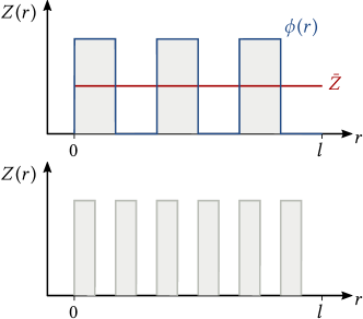
Figure 1: Sketch of two patterns with equal relative entropy. Any transformation $\phi(r)\to\phi^{\prime}(r)=\phi(r^{\prime})$ with $|\partial r/\partial r^{\prime}|=1$, corresponding to a simple rearrangement of the local concentrations, leaves ${\mathcal{L}}(Z|Z^{\rm eq})$ unchanged. This is rooted in the lack of interactions between chemicals at the scale of RDS.

The relative entropy (5) possesses some important physical features. First, in the absence of reactions it gives the total entropy produced by the diffusive expansion of concentrations. For example, consider $n_{\mathrm{A}}$ and $n_{\mathrm{B}}$ moles of inert chemicals A and B initially placed in the volume fractions $V_{\mathrm{A}}$ and $V_{\mathrm{B}}$, respectively. They relax to homogeneous concentrations with an entropy production $-{\mathcal{L}}=n_{\mathrm{A}}\log V_{\mathrm{A}}+n_{\mathrm{B}}\log V_{\mathrm{B}}$ that is exactly the entropy of mixing of the two species *[][; ch.~6.]ben-naim08. It is remarkable that diffusive dissipation and mixing entropy are thus fully described in a purely information theoretic fashion, namely as a relative entropy between concentrations. Second, the relative entropy between reacting concentrations $Z_{\sigma}(\boldsymbol{r},t)=\bar{Z}_{\sigma}(t)\phi_{\sigma}(\boldsymbol{r},t){\mathcal{V}}$ and arbitrary reference homogeneous concentrations $Z_{\sigma}^{\rm h}$ can be split into the relative entropy between space-averaged concentrations $\bar{Z}_{\sigma}(t)=\int_{\mathcal{V}}\mathrm{d}\boldsymbol{r}\,Z_{\sigma}(\boldsymbol{r},t)/{\mathcal{V}}$ and equilibrium ones $Z^{\rm eq}_{\sigma}$, plus the relative entropy of the normalized local modulations $\phi_{\sigma}(\boldsymbol{r})$ around $\bar{Z}_{\sigma}$ and the flat distribution $1/{\mathcal{V}}$:

$${\mathcal{L}}(Z_{\sigma}\|Z_{\sigma}^{\rm h})={\mathcal{L}}(\bar{Z}_{\sigma}\|Z_{\sigma}^{\rm h})+{\textstyle\sum_{\sigma}}\bar{Z}_{\sigma}{\mathcal{L}}(\phi_{\sigma}\|1/{\mathcal{V}}).$$ (8)

The positivity of relative entropy implies ${\mathcal{L}}(Z_{\sigma}\|Z_{\sigma}^{\rm h})\geqslant{\mathcal{L}}(\bar{Z}_{\sigma}\|Z_{\sigma}^{\rm h})$, i.e. the free energy of a patterned system is always larger than its homogeneous counterpart. Third, different patterns may have the same relative entropy (see Fig. 1) indicating that morphology and thermodynamics need not be correlated Serna et al. (2017).

Notice that the conservation laws of the CN are instrumental in the derivation of (4). Indeed, the equilibrium condition ${\sum_{\sigma}}\mathbb{S}^{\sigma}_{\rho}\mu_{\sigma}^{\rm eq}=0$ corresponding to null reaction affinities, $f_{\rho}=0$, implies that $\mu_{\sigma}^{\rm eq}$ is a linear combination of the conservation laws $\ell^{\lambda}_{\sigma}$. This entails $\int_{{\mathcal{V}}}\mathrm{d}\boldsymbol{r}\sum_{\sigma}\mu_{\sigma}^{\rm eq}\partial_{t}Z_{\sigma}=0$, which yields in turn the decomposition (4) when time integrating along a relaxation dynamics leading from $Z_{\sigma}$ to $Z_{\sigma}^{\rm eq}$.

Moreover, the conservation laws are the passkey to construct the correct nonequilibrium thermodynamic potential for open systems. For the latter, an additional term appears when taking the time derivative of $G$ due to the external current in (1),

$$\dot{W}_{\mathrm{chem}}=\int_{\mathcal{V}}\mathrm{d}\boldsymbol{r}\,{\textstyle\sum_{\sigma}}\mu_{\sigma}(\boldsymbol{r})I_{\sigma}(\boldsymbol{r})\,,$$ (9)

which defines the chemical work performed by the chemostats. The second law (6) thus attains the new form

$$\dot{W}_{\mathrm{chem}}-{\mathrm{d}}_{t}G=\dot{\Sigma}\geqslant 0,$$ (10)

where the EPR $\dot{\Sigma}$ is still given by the two contributions of Eq. (7). Consequently, $G$ is no longer minimized due to the break of conservations laws. Similarly to equilibrium thermodynamics when passing from canonical to grand canonical ensembles, one needs to transform the free energy $G$ subtracting the energetic contributions of matter exchanged with the reservoirs Alberty (2003). This amounts to the moieties of the broken components $M_{y_{\mathrm{p}}}={\textstyle\sum_{\lambda_{\mathrm{b}}}}{\ell_{y_{\mathrm{p}}}^{\lambda_{\mathrm{b}}}}^{-1}\int\mathrm{d}\boldsymbol{r}\,L_{\lambda_{\mathrm{b}}}(\boldsymbol{r})$ entering those chemostats $y_{\mathrm{p}}$ that break all conservation laws, times the reference values of their chemical potential $\mu^{\mathrm{ref}}_{y_{\mathrm{p}}}$ (which simplifies to $\mu_{y_{\mathrm{p}}}$ for homogeneous chemostats). The so obtained semigrand Gibbs free energy,

$${\mathcal{G}}=G-{\textstyle\sum_{y_{\mathrm{p}}}}\mu^{\mathrm{ref}}_{y_{\mathrm{p}}}M_{y_{\mathrm{p}}}\,,$$ (11)

encodes CN-specific topological and spatial features thanks to the freedom in the choice of $y_{\mathrm{p}}$ and $\mu^{\mathrm{ref}}_{y_{\mathrm{p}}}$. This allows one to split the EPR

$$\dot{W}_{\mathrm{driv}}+\dot{W}_{\mathrm{nc}}-{\mathrm{d}}_{t}{\mathcal{G}}=\dot{\Sigma}\,,$$ (12)

in terms of the driving and the nonconservative chemical work rate, respectively,

$$\dot{W}_{\mathrm{driv}} =-{\textstyle\sum_{y_{\mathrm{p}}}}{\mathrm{d}}_{t}\mu^{\mathrm{ref}}_{y_{\mathrm{p}}}M_{y_{\mathrm{p}}}\,, \dot{W}_{\mathrm{nc}} ={\textstyle\sum_{y}}\int_{{\mathcal{V}}}\mathrm{d}\boldsymbol{r}I_{y}\mathcal{F}_{y}\,.$$ (13)

The former results from time-dependent manipulations of the reference chemostats $y_{\mathrm{p}}$, while the latter gives the cost of sustaining chemical flows by means of the forces $\mathcal{F}_{y}(\boldsymbol{r})=\mu_{y}(\boldsymbol{r})-{\textstyle\sum_{y_{\mathrm{p}}}}\mu^{\mathrm{ref}}_{y_{\mathrm{p}}}{\textstyle\sum_{\lambda_{\mathrm{b}}}}{\ell_{y_{\mathrm{p}}}^{\lambda_{\mathrm{b}}}}^{-1}\ell_{y}^{\lambda_{\mathrm{b}}}$ measured with respect to the reference chemical potentials $\mu^{\mathrm{ref}}_{y_{\mathrm{p}}}$. Eq. (12) is a major result of this Letter and can be verified by direct substitution.

In absence of driving (${\mathrm{d}}_{t}\mu^{\mathrm{ref}}_{y_{\mathrm{p}}}$=0) and nonconservative forcing (${\mathcal{F}}_{y}=0$) it simplifies to ${\mathrm{d}}_{t}{\mathcal{G}}=-\dot{\Sigma}\leqslant 0$, which proves that the CN, despite being open, relaxes to equilibrium by minimizing the free energy ${\mathcal{G}}$. Moreover, for a generic open CN, the decomposition of ${\mathcal{G}}$ corresponding to (4), i.e. ${\mathcal{G}}-{\mathcal{G}}^{\mathrm{eq}}={\mathcal{L}}(Z_{x}\|Z^{\rm eq}_{x})\geqslant 0$, and a time integral between two nonequilibrium states connected by an arbitrary manipulation turn (12) into a nonequilibrium Landauer principle Esposito and Van den Broeck (2011) for RDS,

$$W_{\mathrm{driv}}+W_{\mathrm{nc}}-\Delta{\mathcal{G}}_{\mathrm{eq}}\geqslant\Delta{\mathcal{L}}(Z_{x}\|Z^{\rm eq}_{x})\,.$$ (14)

The latter states that the dissipative work spent to manipulate the CN is bounded by the variation in relative entropy between the boundary states and their respective equilibria attained by stopping the driving and zeroing the forcing.

Turing pattern in the Brusselator model—As first proposed by A. Turing in his seminal paper Turing (1990), RDS undergo a spatial symmetry braking leading to a stationary pattern when at least two chemical species react nonlinearly and their diffusivities differ substantially. A minimal system that captures these essential features is the Brusselator model Prigogine and Lefever (1968) in one spatial dimension. Here the concentrations of two chemical species, an activator $Z_{X_{1}}=x_{1}(r,t)$ and an inhibitor $Z_{X_{2}}=x_{2}(r,t)$, evolve in time and space $r\in[0,l]$ according to the RDS (1) for the network depicted in Fig. 2, namely,

$$\partial_{t}\begin{pmatrix}x_{1}\\ x_{2}\end{pmatrix}=\underbrace{\begin{pmatrix}k_{1}y_{1}-k_{-1}x_{1}-k_{2}y_{2}x_{1}+k_{-2}y_{3}x_{2}+k_{3}x_{1}^{2}x_{2}-k_{-3}x_{1}^{3}-k_{4}x_{1}+k_{-4}y_{4}+D_{x_{1}}\partial_{r}^{2}x_{1},\\ k_{2}y_{2}x_{1}-k_{-2}y_{3}x_{2}-k_{3}x_{1}^{2}x_{2}+k_{-3}x_{1}^{3}+D_{x_{2}}\partial_{r}^{2}x_{2}\end{pmatrix}}_{\text{\small$={\mathcal{J}}(x_{1},x_{2})$}},$$ (15)

The $y_{1},y_{2},y_{3}$ and $y_{4}$ are the homogeneous concentrations of the chemostatted species and the diffusivities satisfy the Turing condition $D_{x_{1}}\ll D_{x_{2}}$. Equation (15) admits a homogeneous stationary solution $(x_{1}^{\mathrm{h}},x_{2}^{\mathrm{h}})^{\mathsf{T}}$ that becomes unstable for $y_{2}\geqslant y_{2}^{\mathrm{c}}$, so that a sinusoidal pattern with wavelength $q_{\mathrm{c}}$ and amplitude proportional to the (in general complex) function $A(r,t)$ starts developing around the space-averaged concentrations $\bar{x}(t)$ Kondepudi and Prigogine (2014):

$$\begin{pmatrix}x_{1}(r,t)\\ x_{2}(r,t)\end{pmatrix}\!=\!\begin{pmatrix}\bar{x}_{1}(t)\\ \bar{x}_{2}(t)\end{pmatrix}+\begin{pmatrix}1\\ u_{x_{2}}\end{pmatrix}\left(A(r,t)e^{iq_{\mathrm{c}}r}+c.c.\right).$$ (16)

Figure 2: Nonequilibrium semigrand Gibbs free energy ${\mathcal{G}}$ for the Brusselator model as a function of the chemical potential of the chemostatted species $Z_{Y_{2}}$, obtained by the analytic stationary solution of the amplitude equation. To define ${\mathcal{G}}$ we choose $y_{1}$ and $y_{2}$ as the reference chemostats breaking the two components $L_{1}=x_{1}+x_{2}+y_{1}+y_{4}$ and $L_{2}=y_{2}+y_{3}$. The dotted line represents the free energy ${\mathcal{G}}$ in the unstable homogeneous system before the pattern growth. Symbols ($\star$) result from numerical integration of (15). Inset: the derivative $\partial{\mathcal{G}}/\partial\mu_{Y_{2}}$ displays a discontinuity at $y_{2}^{\mathrm{c}}\simeq 2.66$.

Figure 3: Analytical result for the EPR of reaction $\dot{\Sigma}_{\mathrm{rct}}$ (dashed) and diffusion $\dot{\Sigma}_{\mathrm{dff}}$ (solid) in the stable stationary state as function of the concentration $y_{2}$. The EPR of the (unstable for $y_{2}>y_{2}^{\textrm{c}}$) homogeneous state $\dot{\Sigma}^{\rm h}$ is subtracted from the former to show the effect of the pattern formation, i.e. decreasing reaction dissipation at the expense of diffusion dissipation. Inset: The total entropy production shows no singularity at the phase transition. All results correspond to the weakly reversible case $k_{-\rho}=10^{-4}\ll k_{+\rho}=1$, and $y_{3}=y_{4}=10^{-4}$, $y_{1}=2$, $D_{x_{1}}=1$, $D_{x_{2}}=10$.

The critical values $y_{2}^{\mathrm{c}}$ and $q_{\mathrm{c}}$ are determined by the condition of marginal stability of the homogeneous state: they are the smaller values for which the matrix $\partial_{x}{\mathcal{J}}{(x_{1}^{\mathrm{h}},x_{2}^{\mathrm{h}})}$ (evolving linearized perturbations) acquires a zero eigenvalue, the corresponding eigenvector being $(1,u_{x_{2}})^{\mathsf{T}}$. Near the onset of instability one can treat ${\epsilon=(y_{2}-y_{2}^{\mathrm{c}})/y_{2}^{\mathrm{c}}}\ll 1$ as a small parameter and carry out a perturbation expansion in powers of $\epsilon$. This leads to the amplitude equation for $A(r,t)$ Peña and Pérez-García (2001),

$$\tau\partial_{t}A=\epsilon A-\alpha|A|^{2}A+\xi\partial_{r}^{2}A,$$ (17)

which describes an exponential growth from an initial small perturbation $A(r,0)\simeq 0$ followed by a late-time saturation due to the nonlinear terms in (15). Amplitude equations provide a general quantitative description of pattern formation in several systems near the onset of instability Cross and Greenside (2009), irrespective of the details of the underlying physical process that are subsumed into the effective coefficients $\tau$, $\alpha$, and $\xi$. Since (17) can be seen as a gradient flow in a complex Ginzburg–Landau potential, pattern formation is usually considered a dynamical phase transition Aranson and Kramer (2002). Here, using an analytical approximate solution to (15) valid for $\epsilon\ll 1$, we show that the phenomenon is in fact a genuine thermodynamic phase transition identified by the appearance of a kink singularity at $y_{2}^{\mathrm{c}}$ in the nonequilibrium free energy ${\mathcal{G}}(y_{2})$. The semigrand canonical free energy of Fig. 2 is calculated taking the stationary stable solution corresponding to a given value of $y_{2}$, i.e. the homogenous one for $y_{2}\leqslant y_{2}^{\mathrm{c}}$ and the patterned one for $y_{2}>y_{2}^{\mathrm{c}}$, namely

$$\begin{pmatrix}x_{1}^{\mathrm{p}}(r)\\ x_{2}^{\mathrm{p}}(r)\end{pmatrix}\sim\begin{pmatrix}1\\ u_{\mathrm{x_{2}}}\end{pmatrix}\sqrt{\frac{\epsilon}{\alpha}}2\cos(q_{c}r)$$ (18)

The physical meaning of the kink at $y_{2}=y_{2}^{\mathrm{c}}$ is best understood noticing that the quantity $\partial{\mathcal{G}}/\partial\mu_{Y_{2}}=\dot{W}_{\mathrm{driv}}/{\mathrm{d}}_{t}\mu_{Y_{2}}$ is the driving work upon a quasi-static manipulation of the chemical potential $\mu_{Y_{2}}$. Interestingly, the total EPR shows no singularity at the transition (cf. Fig. 3): moving across $y_{2}^{\mathrm{c}}$ the EPR of reaction $\dot{\Sigma}_{\mathrm{rct}}$ decreases with respect to the homogeneous state value $\dot{\Sigma}^{\mathrm{h}}$ while a non zero EPR of diffusion appears, their sum being continuous.

Conclusion—We presented the nonequilibrium thermodynamics of RDS and exemplified the theory with the application to the Brusselator model. We went beyond the conventional treatment of classical nonequilibrium thermodynamics Kjelstrup and Bedeaux (2008) in two respects: avoiding to linearize the chemistry, i.e. to oversimplify reaction affinities to currents times Onsager coefficients; explicitly building thermodynamic potentials that act as Lyapunov functions in the relaxation to equilibrium, provide minimum work principles, and reveal the existence of nonequilibrium phase transitions. The framework paves the way to study the energy cost of pattern manipulation and information transmission in complex chemical systems Zadorin et al. (2015); Epstein and Xu (2016); Halatek and Frey (2018).

We acknowledge funding from the National Research Fund of Luxembourg (AFR PhD Grant 2014-2, No. 9114110) and the European Research Council project NanoThermo (ERC-2015-CoG Agreement No. 681456).

References

- Castets et al. (1990) V. Castets, E. Dulos, J. Boissonade, and P. De Kepper, Phys. Rev. Lett. 64, 2953 (1990).
- Ouyang and Swinney (1991) Q. Ouyang and H. L. Swinney, Nature 352, 610 (1991).
- Zaikin and Zhabotinsky (1970) A. N. Zaikin and A. M. Zhabotinsky, Nature 225, 535 (1970).
- Winfree (1972) A. T. Winfree, Science 175, 634 (1972).
- Ortoleva (1994) P. J. Ortoleva, Geochemical self-organization (Oxford University Press, 1994).
- Murray (2001) J. D. Murray, Mathematical biology. II spatial models and biomedical applications, 3rd ed. (Springer-Verlag, 2001).
- Kondo and Miura (2010) S. Kondo and T. Miura, Science 329, 1616 (2010).
- Kretschmer and Schwille (2016) S. Kretschmer and P. Schwille, Curr. Opin. Cell. Biol. 38, 52 (2016).
- Falcke (2004) M. Falcke, Adv. Phys. 53, 255 (2004).
- Thurley et al. (2012) K. Thurley, A. Skupin, R. Thul, and M. Falcke, Biochim. Biophys. Acta 1820, 1185 (2012).
- Prigogine and Nicolis (1971) I. Prigogine and G. Nicolis, Q. Rev. Biophys. 4, 107 (1971).
- Nicolis and Prigogine (1977) G. Nicolis and I. Prigogine, Self-organization in Nonequilibrium Systems: From Dissipative Structures to Order Through Fluctuations (Wiley-Blackwell, 1977).
- Cross and Hohenberg (1993) M. C. Cross and P. C. Hohenberg, Rev. Mod. Phys. 65, 851 (1993).
- Ross (2008) J. Ross, Thermodynamics and Fluctuations far from Equilibrium (Springer, 2008).
- Rossi et al. (2008) F. Rossi, S. Ristori, M. Rustici, N. Marchettini, and E. Tiezzi, J. Theor. Biol. 255, 404 (2008).
- Grzybowski and Huck (2016) B. A. Grzybowski and W. T. Huck, Nat. Nanotechnol. 11, 585 (2016).
- Adamatzky et al. (2005) A. Adamatzky, B. De Lacy Costello, and T. Asai, Reaction-diffusion computers (Elsevier, 2005).
- Jarzynski (2011) C. Jarzynski, Annu. Rev. Condens. Matter Phys. 2, 329 (2011).
- Seifert (2012) U. Seifert, Rep. Prog. Phys. 75, 126001 (2012).
- Van den Broeck and Esposito (2015) C. Van den Broeck and M. Esposito, Physica A 418, 6 (2015).
- Rao and Esposito (2016) R. Rao and M. Esposito, Phys. Rev. X 6, 041064 (2016).
- Polettini and Esposito (2014) M. Polettini and M. Esposito, J. Chem. Phys. 141, 024117 (2014).
- Polettini et al. (2016) M. Polettini, G. Bulnes Cuetara, and M. Esposito, Phys. Rev. E 94, 052117 (2016).
- Rao and Esposito (2018) R. Rao and M. Esposito, New J. Phys. 20, 023007 (2018).
- Haraldsdóttir and Fleming (2016) H. S. Haraldsdóttir and R. M. T. Fleming, PLoS Comput Biol 12, e1004999 (2016).
- de Groot and Mazur (1984) S. R. de Groot and P. Mazur, Non-equilibrium Thermodynamics (Dover, 1984).
- Kondepudi and Prigogine (2014) D. Kondepudi and I. Prigogine, Modern Thermodynamics: From Heat Engines to Dissipative Structures, 2nd ed. (Wiley, 2014).
- Esposito and Van den Broeck (2011) M. Esposito and C. Van den Broeck, Europhys. Lett. 95, 40004 (2011).
- Ben-Naim (2008) A. Ben-Naim, A Farewell To Entropy: Statistical Thermodynamics Based On Information (World Scientific Publishing Company, 2008).
- Serna et al. (2017) H. Serna, A. P. Muñuzuri, and D. Barragán, Phys. Chem. Chem. Phys. 19, 14401 (2017).
- Alberty (2003) R. A. Alberty, Thermodynamics of biochemical reactions (Wiley-Interscience, 2003).
- Turing (1990) A. Turing, Bull. Math. Biol. 52, 153 (1990).
- Prigogine and Lefever (1968) I. Prigogine and R. Lefever, J. Chem. Phys. 48, 1695 (1968).
- Peña and Pérez-García (2001) B. Peña and C. Pérez-García, Phys. Rev. E 64, 056213 (2001).
- Cross and Greenside (2009) M. Cross and H. Greenside, Pattern formation and dynamics in nonequilibrium systems (Cambridge University Press, 2009).
- Aranson and Kramer (2002) I. S. Aranson and L. Kramer, Rev. Mod. Phys. 74, 99 (2002).
- Kjelstrup and Bedeaux (2008) S. Kjelstrup and D. Bedeaux, Non-equilibrium thermodynamics of heterogeneous systems, Vol. 16 (World Scientific, 2008).
- Zadorin et al. (2015) A. S. Zadorin, Y. Rondelez, J.-C. Galas, and A. Estevez-Torres, Phys. Rev. Lett. 114, 068301 (2015).
- Epstein and Xu (2016) I. R. Epstein and B. Xu, Nat. Nanotechnol. 11, 312 (2016).
- Halatek and Frey (2018) J. Halatek and E. Frey, Nat. Phys. , 1 (2018).